Clustering Under Prior Knowledge with Application to Image Segmentation
Cluster assignment strategies for a clustered trace cache processor
Cluster Assignment Strategiesfor a Clustered Trace Cache ProcessorRavi Bhargava and Lizy K.JohnTechnical Report TR-033103-01Laboratory for Computer ArchitectureThe University of Texas at AustinAustin,Texas,78712{ravib,ljohn}@March31,2003AbstractThis report examines dynamic cluster assignment for a clustered trace cache processor(CTCP).Previously proposed clustering techniques run into unique problems as issue width and clustercount increase.Realistic design conditions,such as variable data forwarding latencies betweenclusters and a heavily partitioned instruction window also increase the degree of difficulty foreffective cluster assignment.In this report,the trace cache andfill unit are used to perform effective dynamic cluster as-signment.The retire-timefill unit analysis is aided by a dynamic profiling mechanism embeddedwithin the trace cache.This mechanism provides information on inter-trace trace dependen-cies and critical inputs,elements absent in previous retire-time CTCP cluster assignment work.The strategy proposed in this report leads to more intra-cluster data forwarding and shorterdata forwarding distances.In addition,performing this strategy at retire-time reduces issue-time complexity and eliminates early pipeline stages.This increases overall performance for theSPEC CPU2000integer programs by8.4%over our base CTCP architecture.This speedup issignificantly higher than a previously proposed retire-time CTCP assignment strategy(1.9%).Dynamic cluster assignment is also evaluated for several alternate cluster designs as well asmedia benchmarks.1IntroductionA clustered microarchitecture design allows for wide instruction execution while reducing the amount of complexity and long-latency communication[2,3,5,7,11,21].The execution resources and registerfile are partitioned into smaller and simpler units.Within a cluster,communication is fast while inter-cluster communication is more costly.Therefore,the key to high performance on a clustered microarchitecture is assigning instructions to clusters in a way that limits inter-cluster data communication.During cluster assignment,an instruction is designated for execution on a particular cluster. This assignment process can be accomplished statically,dynamically at issue-time,or dynamicallyat retire-time.Static cluster assignment is traditionally done by a compiler or assembly programmer and may require ISA modification and intimate knowledge of the underlying cluster hardware. Studies that have compared static and dynamic assignment conclude that dynamic assignment results in higher performance[2,15].Dynamic issue-time cluster assignment occurs after instructions are fetched and decoded.In recent literature,the prevailing philosophy is to assign instructions to a cluster based on data de-pendencies and workload balance[2,11,15,21].The precise method varies based on the underlying architecture and execution cluster characteristics.Typical issue-time cluster assignment strategies do not scale well.Dependency analysis is an inherently serial process that must be performed in parallel on all fetched instructions.Therefore, increasing the width of the microarchitecture further delays and frustrates this dependency anal-ysis(also noted by Zyuban et al.[21]).Accomplishing even a simple steering algorithm requires additional pipeline stages early in the instruction pipeline.In this report,the clustered execution architecture is combined with an instruction trace cache, resulting in a clustered trace cache processor(CTCP).A CTCP achieves a very wide instruction fetch bandwidth using the trace cache to fetch past multiple branches in a low-latency and high-bandwidth manner[13,14,17].The CTCP environment enables the use of retire-time cluster assignment,which addresses many of the problems associated with issue-time cluster assignment.In a CTCP,the issue-time dynamic cluster assignment logic and steering network can be removed entirely.Instead,instructions are issued directly to clusters based on their physical instruction order in an trace cache line or instruc-tion cache block.This eliminates critical latency from the front-end of the pipeline.Instead,cluster assignment is accomplished at retire-time by physically(but not logically)reordering instructions so that they are issued directly to the desired cluster.Friendly et al.present a retire-time cluster assignment strategy for a CTCP based on intra-trace data dependencies[6].The trace cachefill unit is capable of performing advanced analysis since the latency at retire-time is more tolerable and less critical to performance[6,8].The shortcoming of this strategy is the loss of dynamic information.Inter-trace dependencies and workload balance information are not available at instruction retirement and are ignored.In this report,we increase the performance of a wide issue CTCP using a feedback-directed, retire-time(FDRT)cluster assignment strategy.Extrafields are added to the trace cache to accu-mulate inter-trace dependency history,as well as the criticality of instruction inputs.Thefill unit combines this information with intra-trace dependency analysis to determine cluster assignments.This novel strategy increases the amount of critical intra-cluster data forwarding by44%while decreasing the average data forwarding distance by35%over our baseline four-cluster,16-way CTCP.This leads to a8.4%improvement in performance over our base architecture compared to 1.9%improvement for Friendly’s method.2Clustered MicroarchitectureA clustered microarchitecture is designed to reduce the performance bottlenecks that result from wide-issue complexity[11].Structures within a cluster are small and data forwarding delays are reduced as long as communication takes place within the cluster.The target microarchitecture in this report is composed of four,four-way clusters.Four-wide, out-of-order execution engines have proven manageable in the past and are the building blocks of previously proposed two-cluster microarchitectures.Similarly configured16-wide CTCP’s have been studied[6,21],but not with respect to the performance of dynamic cluster assignment options.An example of the instruction and data routing for the baseline CTCP is shown in Figure1. Notice that the cluster assignment for a particular instruction is dependent on its placement in the instruction buffer.The details of a single cluster are explored later in Figure3Figure1:Overview of a Clustered Trace Cache ProcessorC2and C3are clusters identical to Cluster1and Cluster4.2.1Shared ComponentsThe front-end of the processor(i.e.fetch and decode)is shared by all of the cluster resources. Instructions fetched from the trace cache(or from the instruction cache on a trace cache miss)are decoded and renamed in parallel beforefinally being distributed to their respective clusters.The memory subsystem components,including the store buffer,load queue,and data cache,are also shared.Pipeline The baseline pipeline for our microarchitecture is shown in Figure2.Three pipeline stages are assigned for instruction fetch(illustrated as one box).After the instructions are fetched, there are additional pipeline stages for decode,rename,issue,dispatch,and execute.Registerfile accesses are initiated during the rename stage.Memory instructions incur extra stages to access the TLB and data cache.Floating point instructions and complex instructions(not shown)alsoexecution.endure extra pipeline stages forTrace Cache The trace cache allows multiple basic blocks to be fetched with just one request[13, 14,17].The retired instruction stream is fed to thefill unit which constructs the traces.These traces consist of up to three basic blocks of instructions.When the traces are constructed,the intra-trace and intra-block dependencies are analyzed.This allows thefill unit to add bits to the trace cache line which accelerates register renaming and instruction steering[13].This is the mechanism which is exploited to improve instruction reordering and cluster assignment.2.2Cluster DesignThe execution resources modeled in this report are heavily partitioned.As shown in Figure3,each cluster consists offive reservation stations which feed a total of eight special-purpose functional units.The reservation stations hold eight instructions and permit out-of-order instruction selec-tion.The economical size reduces the complexity of the wake-up and instruction select logic while maintaining a large overall instruction window size[11].Figure3:Details of One ClusterThere are eight special-purpose functional units per cluster:two simple integer units,one integermemory unit,one branch unit,one complex integer unit,one basicfloating point(FP),one complexFP,one FP memory.There arefive8-entry reservation stations:one for the memory operations(integer and FP),one for branches,one for complex arithmetic,two for the simple operations.FPis not shown.Intra-cluster communication(i.e.forwarding results from the execution units to the reservation stations within the same cluster)is done in the same cycle as instruction dispatch.However,to forward data to a neighboring cluster takes two cycles and beyond that another two cycles.This latency includes all of the communication and routing overhead associated with sharing inter-cluster data[12,21].The end clusters do not communicate directly.There are no data bandwidth limitations between clusters in our work.Parcerisa et al.show that a point-to-point interconnect network can be built efficiently and is preferable to bus-based interconnects[12].2.3Cluster AssignmentThe challenge to high performance in clustered microarchitectures is assigning instructions to the proper cluster.This includes identifying which instruction should go to which cluster and then routing the instructions accordingly.With16instructions to analyze and four clusters from whichto choose,picking the best execution resource is not straightforward.Accurate dependency analysis is a serial process and is difficult to accomplish in a timely fashion.For example,approximately half of all result-producing instructions have data consumed by an instruction in the same cache line.Some of this information is preprocessed by thefill unit, but issue-time processing is also required.Properly analyzing the relationships is critical but costly in terms of pipe stages.Any extra pipeline stages hurt performance when the pipeline refills after branch mispredictions and instruction cache misses.Totallyflexible routing is also a high-latency process.So instead,our baseline architecture steers instructions to a cluster based on its physical placement in the instruction buffer.Instructions are sent in groups of four to their corresponding cluster where they are routed on a smaller crossbar to their proper reservation station.This style of partitioning results in less complexity and fewer potential pipeline stages,but is restrictive in terms of issue-timeflexibility and steering power.A large crossbar will permit instruction movement from any position in the instruction buffer to any of the clusters.In addition to the latency and complexity drawbacks,this option mandates providing enough reservations stations write ports to accommodate up to16new instructions per cycle.Therefore,we concentrate on simpler,low-latency instruction steering.Assignment Options For comparison purposes,we look at the following dynamic cluster assign-ment options:•Issue-Time:Instructions are distributed to the cluster where one or more of their input data is known to be generated.Inter-trace and intra-trace dependencies are visible.A limit of four instructions are assigned to each cluster every cycle.Besides simplifying hardware, this also balances the cluster workloads.This option is examined with zero latency and with four cycles of latency for dependency analysis,instruction steering,and routing.•Friendly Retire-Time:This is the only previously proposedfill unit cluster assignment policy.Friendly et al.propose afill unit reordering and assignment scheme based on intra-trace dependency analysis[6].Their scheme assumes a front-end scheduler restricted to simple slot-based issue,as in our base model.For each issue slot,each instruction is checked for an intra-trace input dependency for the respective cluster.Based on these data dependencies, instructions are physically reordered within the trace.3CTCP CharacteristicsThe following characterization serves to highlight the cluster assignment optimization opportunities.3.1Trace-level AnalysisTable1presents some run-time trace line characteristics for our benchmarks.Thefirst metric(% TC Instr)is the percentage of all retired instructions fetched from the trace cache.Benchmarks with a large percentage of trace cache instructions benefit more fromfill unit optimizations since instructions from the instruction cache are unoptimized for the CTCP.Trace Size is the average number of instructions per trace line.When thefill unit does the intra-trace dependency analysis for a trace,this is the available optimization scope.Table1:Trace CharacteristicsTrace Size99.31craft y10.8772.63gap11.7569.66gzip11.7996.61parser9.0286.43twolf10.3273.77vpr11.1084.310%20%40%60%80%100%bzp crf eon gap gcc gzp mcf psr prl twf vor vpr%D y n a m i c I n s t r u c t i o n s W i t h I n p u t sFigure 4:Source of Critical Input DependencyFrom RS2:Critical input provided by the producer for input RS2.From RS1:Critical input provided by the producer for input RS1.From RF:Critical input provided by the register file.Table 2:Dynamic Consumers Per InstructionInter-Trace0.90crafty0.270.82gap0.241.03gzip0.300.54parser0.501.17twolf0.331.00vpr0.331.03Table3:Critical Data Forwarding Dependencies%of critical dep.’sthat are inter-trace85.63%crafty24.32%86.58%gap22.72%87.59%gzip24.38%89.62%parser38.16%86.11%twolf23.95%85.51%vpr25.84%84.91%1For bzip2,the branch predictor accuracy is sensitive to the rate at which instructions retire and the“better”case with no data forwarding latency actually leads to an increase in branch mispredictions and worse performance.the registerfile read latency is presented and has almost no effect on overall performance.In fact, registerfile latencies between zero and10cycles have no impact on performance.This is due to the abundance and critical nature of in-flight instruction data forwarding.3.3Resolving Inter-Trace DependenciesThefill unit accurately determines intra-trace dependencies.Since a trace is an atomic trace cache unit,the same intra-trace instruction data dependencies will exist when the trace is later fetched. However,incorporating inter-trace dependencies at retire-time is essentially a prediction of issue-time dependencies,some of which may occur thousands or millions of cycles in the future.This problem presents an opportunity for an execution history based mechanism to predict the source clusters or producers for instructions with inter-trace dependencies.Table4examines the how often an instruction’s forwarded data comes from the same producer instruction.For each static instruction,the program counter of the last producer is tracked for each source register(RS1 and RS2).The table shows that an instruction’s data forwarding producer is the same for RS1 96.3%of the time and the same for RS294.3%of the time.Table4:Frequency of Repeated Forwarding ProducersAll Critical Inter-traceInput RS1Input RS2Input RS1Input RS297.44%89.30%crafty97.82%93.55%93.83%85.79%gap93.65%77.88%96.39%85.36%gzip99.02%96.04%96.61%92.36%parser87.66%78.76%97.78%90.83%twolf90.78%76.40%89.67%70.87%vpr96.06%91.67%96.25%86.92%Inter-trace dependencies do not necessarily arrive from the previous trace.They could arrive from any trace in the past.In addition,static instructions are sometimes incorporated into several different dynamic traces.Table5analyzes the distance between an instruction and its critical inter-trace producer.The values are the percentage of such instructions that encounter the same distance in consecutive executions.This percentage correlates very well to the percentages in the last two columns of Table4.On average,85.9%of critical inter-trace forwarding is the same distance from a producer as the previoue dynamic instance of the instruction.Table5:Frequency of Repeated Critical Inter-Trace Forwarding Distancesbzip2craftyeongapgccgzipmcfparserperlbmktwolfvortexvprAveragedecrease.The important aspect is that physical reordering reduces inter-cluster communications while maintaining low-latency,complexity-effective issue logic.4.1Pinning InstructionsPhysically reordering instructions at retire-time based on execution history can cause more inter-cluster data forwarding than it eliminates.When speculated inter-trace dependencies guide the reordering strategy,the same trace of instructions can be reordered in a different manner each time the trace is constructed.Producers shift from one cluster to another,never allowing the consumers to accurately gauge the cluster from which their input data will be produced.A retire-time instruction reordering heuristic must be chosen carefully to avoid unstable cluster assignments and self-perpetuating performance problems.To combat this problem,we pin key producers and their subsequent inter-trace consumers to the same cluster to force intra-cluster data forwarding between inter-trace dependencies.This creates a pinned chain of instructions with inter-trace dependencies.Thefirst instruction of the pinned chain is called a leader.The subsequent links of the chain are referred to as followers.The criteria for selecting pin leaders and followers are presented in Table6.Table6:Leader and Follower CriteriaConditions to become a pin leader:1.Not already a leader or follower2.Producer provides last input data3.Producer is a leader or follower4.Producer is from different traceThere are two key aspects to these guidelines.Thefirst is that only inter-trace dependencies are considered.Placing instructions with intra-trace dependencies on the same cluster is easy and reliable.Therefore,these instructions do not require the pinned chain method to establish dependencies.Second,once an instruction is assigned to a pinned chain as a leader or a follower,its status should not change.The idea is to pin an instruction to one cluster and force the other instructions in the inter-trace dependency chain to follow it to that same cluster.If the pinned cluster is allowed to change,then it could lead to performance-limiting race conditions discussed earlier.Table7:FDRT Cluster Assignment StrategyDependency typeif...if...if...if...if...Intra-trace producer:no yes yes no no Intra-trace consumer:1.producer 1.pin 1.pin 1.middle 1.skipAssignment Priority:3.skip 3.skip 3.neighbor2Using Cacti2.0[16],an additional byte per instruction in a trace cache line is determined not to change the fetch latency of the trace cache.4.3Cluster Assignment StrategyThefill unit must weigh intra-trace information along with the inter-trace feedback from the trace cache execution histories.Table7summarizes our proposed cluster assignment policies.The inputs to the strategy are:1)the presence of an intra-trace dependency for the instruction’s most critical source register(i.e.the input that was satisfied last during execution),2)the pin chain status, and3)the presence of intra-trace consumers.Thefill unit starts with the oldest instruction and progresses in logical order to the youngest instruction.For option A in Table7,thefill unit attempts to place instructions that have only an intra-trace dependency on the same cluster as its producer.If there are no instruction slots available for the producer’s cluster,an attempt is made to assign the instruction to a neighboring cluster.For an instruction with just an inter-trace pin dependency(option B),thefill unit attempts to place the instruction on the pinned cluster(which is found in the Pinned Cluster trace profilefield)or a neighboring cluster.An instruction can have both an intra-trace dependency and a pinned inter-trace dependency (option C).Recall that pinning an instruction is irreversible.Therefore,if the critical input changes or an instruction is built into a new trace,an intra-trace dependency could exist along with a pinned inter-trace dependency.When an instructions has both a pinned cluster and an intra-trace producer,the pinned cluster takes precedence(although our simulations show that it doesn’t matter which gets precedence).If four instructions have already been assigned to this cluster,the intra-trace producer’s cluster is the next target.Finally,there is an attempt to assign the instruction to a pinned cluster neighbor.If an instruction has no dynamically forwarded input data but does have an intra-trace output dependency(option D),it is assigned to a middle cluster(to reduce potential forwarding distances).Instructions are skipped if they have no input or output dependencies(option E),or if they cannot be assigned to a cluster near their producer(lowest priority assignment for options A-D). These instructions are later assigned to the remaining slots using Friendly’s method.4.4ExampleA simple illustration of the FDRT cluster assignment strategy is shown in Figure6.There are two traces,T1and T2.Trace T1is the older of the two traces.Four instructions(out of at least10)of each trace are shown.Instruction I7is older than instruction I10.The arrows indicate dependencies. The arrows originate at the producer and go to the consumer.A solid black arrowhead represents an intra-trace dependence and a white arrowhead represents an inter-trace dependence.A solidarrow line represents a critical input,and a dashed line represents a non-critical input.Arrows with numbers adjacent to them are chain dependencies where the number represents the chain clusterpinned.to which the instructions should beThe upper portion of this example examines four instructions from the middle of two different traces.The instruction numberings are in logical order.The arrows indicate dependencies,traveling fromthe producer to the consumer.The instructions are assigned to clusters2and3based on theirdependencies.The letterings in parenthesis match those in Table7.Instruction T1I8has one intra-trace producer(Option A),and is assigned to the same cluster as its producer TIdependencies(Option B).The chain cluster value is3,so these instructions are assigned to that cluster.Note that the intra-trace input to T1I7follows Option B and is assigned to Cluster3based on its chain inter-trace dependency.Instruction T2I9and T2I7 and T2Table8:SPEC CINT2000Benchmarks Benchmark InputsMinneSPECcrafty crafty.inSPEC testgap-q-m64M test.inMinneSPECgzip smred.log1MinneSPECparser 2.1.dict-batch mdred.inMinneSPECtwolf mdredMinneSPECvpr small.arch.in-nodisp-place t5-exit t0.9412-innerL1Data Cache:4-way,32KB,2-cycle accessL2Unified cache:4-way,1MB,+8cyclesNon-blocking:16MSHRs and4portsD-TLB:128-entry,4-way,1-cyc hit,30-cyc miss Store buffer:32-entry w/load forwardingLoad queue:32-entry,no speculative disambiguation Main Memory:Infinite,+65cyclesFetch Engine ·Functional unit#t.Issue lat. Simple Integer21cycle1cycle Simple FP231 Memory111Int.Mul/Div13/201/19FP Mul/Div/Sqrt13/12/241/12/24Int Branch111FP Branch111·Inter-Cluster Forwarding Latency:2cycles per forward ·Register File Latency:2cycles·5Reservation stations·8entries per reservation station·2write ports per reservation station·192-entry ROB·Fetch width:16·Decode width:16·Issue width:16·Execute width:16·Retire width:165.2Performance AnalysisFigure7presents the speedups over our base architecture for different dynamic cluster assignment strategies.The proposed feedback-directed,retire-time(FDRT)cluster assignment strategy pro-vides a 7.3%improvement.Friendly’s method improves performance by 1.9%3.This improvement in performance is due to enhancements in both the intra-trace and inter-trace aspects of cluster as-signment.Additional simulations (not shown)show that isolating the intra-trace heuristics from the FDRT strategy results in a 3.4%improvement by itself.The remaining performance improvement generated by FDRT assignment comes from the inter-traceanalysis.0.900.951.001.051.101.151.201.251.301.351.40bzpgcccrfeongapgzpmcfpsrprltwfvorvprHMFigure 7:Speedup Due to Different Cluster Assignment StrategiesThe performance boost is due to an increase in intra-cluster forwarding and a reduction in average data forwarding distance.Table 10presents the changes in intra-cluster forwarding.On average,both CTCP retire-time cluster assignment schemes increase the amount of same-cluster forwarding to above 50%,with FDRT assignment doing better.The inter-cluster distance is the primary cluster assignment performance-related factor (Ta-ble 11).For every benchmark,the retire-time instruction reordering schemes are able to improve upon the average forwarding distance.In addition,the FDRT scheme always provides shorter overall data forwarding distances than the Friendly method.This is a result of funneling producers with no input dependencies to the middle clusters and placing consumers as close as possible to their producers.For the program eon ,the Friendly strategy provides a higher intra-cluster forwarding percent-age than FDRT without resulting in higher performance.The reasons for this are two-fold.MostTable10:Percentage of Intra-Cluster Forwarding For Critical InputsFriendlybzip260.84%crafty54.29%eon52.83%gap58.77%gcc58.14%gzip53.91%mcf64.69%parser57.67%perlbmk58.36%twolf56.91%vortex54.00%vpr58.70%Average57.43%Base FDRT0.830.240.900.590.960.700.710.490.710.510.940.560.620.440.690.530.780.490.730.560.780.520.920.570.800.52Distance is the number of clusters traversed by forwarded data.importantly,the average data forwarding distance is reduced compared to the Friendly method de-spite the extra inter-cluster forwarding.There are also secondary effects that result from improving overall forwarding latency,such as a change in the update rate for the branch predictor and BTB. In this case,our simulations show that FDRT scheme led to improved branch prediction as well.The two retire-time instruction reordering strategies are also compared to issue-time instruction steering in Figure7.In one case,instruction steering and routing is modeled with no latency (labeled as No-lat Issue-time)and in the other case,four cycles are modeled(Issue-time).The results show that latency-free issue-time steering is the best,with a9.9%improvement over the base.However,when applying an aggressive four-cycle latency,issue-time steering is only preferable for three of the12benchmarks and the average performance improvement(3.8%)is almost half that of FDRT cluster assignment.5.3FDRT Assignment AnalysisFigure 8is a breakdown of instructions based on their FDRT assignment strategy option.On average 32%have only an intra-trace dependency,while 16%of the instructions have just an inter-trace pinned dependency.Only 7%of the instructions have both a pin inter-trace dependency and a critical intra-trace dependency.Therefore,55%of the instructions are considered to be consumers and are therefore placed near theirproducers.0%10%20%30%40%50%60%70%80%90%100%bzpcrf eon gap gcc gzp mcf psrprltwfvor vpr AvgFigure 8:FDRT Critical Input DistributionThe letters A-E correspond to the lettered options in Table 7.Around 10%of the instructions had no input dependencies but did have an intra-trace consumer.These producer instructions are assigned to a middle cluster where their consumers will be placed on the same cluster later.Only a very small percentage (less than 1%)of instructions with identified input dependencies are initially skipped because their is no suitable neighbor cluster for assignment.Finally,a large percentage of instructions (around 34%)are determined to not have a critical intra-trace dependency or pinned inter-trace dependency.Most of these instructions do have data dependencies,but they did not require data forwarding or did not meet the pin criteria.Table 12presents pinned chain characteristics,including the average number of leaders per trace and average number of followers per trace.Because pin dependencies are limited to inter-trace dependencies,the combined number of leaders and followers is only 2.90per trace.This is about 1/4of the instructions in a trace.For some of the options in Table 7,the fill unit cluster assignment mechanism attempts to place。
推理正确率分布曲线 英文

推理正确率分布曲线英文English:The distribution curve of inference accuracy represents the spread of correct inference rates across a population or dataset. This curve typically takes the shape of a bell curve, with the majority of individuals or data points clustering around the mean accuracy rate, and fewer individuals or data points at the extremes of high and low accuracy. The central tendency of this curve is indicative of the average accuracy level, while the spread or standard deviation reflects the variability or consistency of inference accuracy within the population or dataset. Factors such as cognitive ability, prior knowledge, experience, and task complexity can influence the shape and parameters of the accuracy distribution curve. In educational settings, understanding the distribution of inference accuracy can inform instructional strategies, curriculum design, and assessment practices, allowing educators to tailor interventions and support to meet the diverse needs of learners. Additionally, in fields like psychology and neuroscience, analyzing individual differences in inference accuracy distribution can shed light on cognitive processes,learning mechanisms, and neural substrates underlying reasoning and decision-making.Translated content:推理正确率分布曲线代表了在人群或数据集中正确推理率的分布情况。
抽样方案的种类包括什么

抽样方案的种类包括什么抽样方案的种类包括什么摘要:抽样是统计学中的一项重要方法,用于从总体中选择一部分样本进行研究和分析。
抽样方案的选择和设计对于研究结果的准确性和可靠性具有决定性的影响。
本文将介绍抽样方案的种类,包括简单随机抽样、系统抽样、整群抽样、分层抽样、多阶段抽样和方便抽样,并对其特点和应用进行详细阐述。
一、简单随机抽样简单随机抽样是最基本的抽样方法,是通过随机抽取每个样本的概率相等,且相互独立的方法。
该方法的优点是样本选择的公平性和随机性,能够较好地代表总体的特征。
然而,由于随机性的特点,样本容易出现偏差,因此需要在实际应用中进行适当的校正和控制。
二、系统抽样系统抽样是按照一定的规则和顺序从总体中抽取样本的方法。
该方法的优点是简单、快捷,能够保持总体的一定特征,并且可以避免简单随机抽样中可能出现的偏差。
然而,如果总体中存在周期性或规律性的特征,系统抽样可能导致样本偏差。
三、整群抽样整群抽样是将总体划分为若干个互不重叠的群体,然后从每个群体中选择部分群体进行抽样的方法。
该方法的优点是能够更好地反映总体的特征,并且减少样本选择的复杂性。
然而,由于群体内的个体可能存在差异,整群抽样可能导致样本的偏差。
四、分层抽样分层抽样是将总体划分为若干个相互独立的层次,然后从每个层次中选择部分样本进行抽样的方法。
该方法的优点是能够在样本选择中考虑到不同层次的差异,增加样本的多样性,并且可以更好地反映总体的特征。
然而,分层抽样需要事先知道总体的分层特征,否则可能导致样本的偏差。
五、多阶段抽样多阶段抽样是将总体分为多个阶段,然后在每个阶段中选择部分样本进行抽样的方法。
该方法的优点是能够逐步缩小样本范围,减少样本选择的复杂性,并且节约时间和成本。
然而,多阶段抽样可能导致样本的聚集性和偏差,需要在设计中合理考虑和控制。
六、方便抽样方便抽样是基于研究者的便利性和容易获得的样本进行抽样的方法。
该方法的优点是简单、快捷,适用于一些初步研究或实践中的问题。
Generalization in clustering with unobserved features

Generalization in Clustering with UnobservedFeaturesEyal Krupka and Naftali TishbySchool of Computer Science and Engineering,Interdisciplinary Center for Neural ComputationThe Hebrew University Jerusalem,91904,Israel{eyalkr,tishby}@cs.huji.ac.ilAbstractWe argue that when objects are characterized by many attributes,clus-tering them on the basis of a relatively small random subset of theseattributes can capture information on the unobserved attributes as well.Moreover,we show that under mild technical conditions,clustering theobjects on the basis of such a random subset performs almost as well asclustering with the full attribute set.We prove afinite sample general-ization theorems for this novel learning scheme that extends analogousresults from the supervised learning setting.The scheme is demonstratedfor collaborativefiltering of users with movies rating as attributes.1IntroductionData clustering is unsupervised classification of objects into groups based on their similar-ity[1].Often,it is desirable to have the clusters to match some labels that are unknown to the clustering algorithm.In this context,a good data clustering is expected to have ho-mogeneous labels in each cluster,under some constraints on the number or complexity of the clusters.This can be quantified by mutual information(see e.g.[2])between the ob-jects’cluster identity and their(unknown)labels,for a given complexity of clusters.Since the clustering algorithm has no access to the labels,it is unclear how the algorithm can optimize the quality of the clustering.Even worse,the clustering quality depends on the specific choice of the unobserved labels.For example a good documents clustering with respect to topics is very different from a clustering with respect to authors.In our setting,instead of trying to cluster by some“arbitrary”labels,we try to predict unobserved features from observed ones.In this sense our target“labels”are yet other features that“happened”to be unobserved.For example,when clustering fruits based on their observed features,such as shape,color and size,the target of clustering is to match unobserved features,such as nutritional value and toxicity.In order to theoretically analyze and quantify this new learning scheme,we make the fol-lowing assumptions.Consider an infinite set of features,and assume that we observe only a random subset of n features,called observed features.The other features are called un-observed features.We assume that the random selection of features is done uniformly and independently.Table1:Analogy with supervised learningTraining set n randomly selected features(observed features)Test set Unobserved featuresLearning algorithm Cluster the instances into k clustersHypothesis class All possible partitions of m instances into k clustersMin generalization error Max expected information on unobserved featuresERM Observed Information Maximization(OIM)Good generalization Mean observed and unobserved information are similar The clustering algorithm has access only to the observed features of m instances.After theclustering,one of the unobserved features is randomly and uniformly selected to be a targetlabel,i.e.clustering performance is measured with respect to this feature.Obviously,theclustering algorithm cannot be directly optimized for this specific feature.The question is whether we can optimize the expected performance on the unobservedfeature,based on the observed features alone.The expectation is over the random selectionof the target feature.In other words,can wefind clusters that match as many unobservedfeatures as possible?Perhaps surprisingly,for large enough number of observed features,the answer is yes.We show that for any clustering algorithm,the average performance ofthe clustering with respect to the observed and unobserved features,is similar.Hence wecan indirectly optimize clustering performance with respect to the unobserved features,inanalogy to generalization in supervised learning.These results are universal and do notrequire any additional assumptions such as underling model or a distribution that createdthe instances.In order to quantify these results,we define two terms:the average observed informa-tion and the expected unobserved information.Let T be the variable which represents thecluster for each instance,and{X1,...,X∞}the set of random variables which denotes the features.The average observed information,denoted by I ob,is the average mutual informa-tion between T and each of the observed features.In other words,if the observed featuresare{X1,...,X n}then I ob=1 n j=1I(T;X j).The expected unobserved information, denoted by I un,is the expected value of the mutual information between T and a randomly selected unobserved feature,i.e.E j{I(T;X j)}.Note that whereas I ob can be measured directly,this paper deals with the question of how to infer and maximize I un.Our main results consist of two theorems.Thefirst is a generalization theorem.It givesan upper bound on the probability of large difference between I ob and I un for all possibleclusterings.It also states a uniform convergence in probability of|I ob−I un|as the num-ber of observed features increases.Conceptually,the observed mean information,I ob,is analogous to the training error in standard supervised learning[3],whereas the unobserved information,I un,is similar to the generalization error.The second theorem states that under constraint on the number of clusters,and large enoughnumber of observed features,one can achieve nearly the best possible performance,interms of I un.Analogous to the principle of Empirical Risk Minimization(ERM)in statis-tical learning theory[3],this is done by maximizing I ob.Table1summarizes the correspondence of our setting to that of supervised learning.Thekey difference is that in supervised learning,the set of features isfixed and the traininginstances(samples)are assumed to be randomly drawn from some distribution.In oursetting,the set of instances isfixed,but the set of observed features is assumed to berandomly selected.Our new theorems are evaluated empirically in section3,on a data set of movie ratings.This empirical test also suggests one future research direction:use the framework sug-gested in this paper for collaborativefiltering.Our main point in this paper,however,is the new conceptual framework and not a specific algorithm or experimental performance. Related work The idea of an information tradeoff between complexity and information on target variables is similar to the idea of the information bottleneck[4].But unlike the bottleneck method,here we are trying to maximize information on unobserved variables, usingfinite samples.In the framework of learning with labeled and unlabeled data[5],a fundamental issue is the link between the marginal distribution P(x)over examples x and the conditional P(y|x) for the label y[6].From this point of view our approach assumes that y is a feature in itself. 2Mathematical Formulation and AnalysisConsider a set of discrete random variables{X1,...,X L},where L is very large(L→∞).We randomly,uniformly and independently select n<<√variables from this set. These variables are the observed features and their indexes are denoted by{q1,...,q n}.The remaining L−n variables are the unobserved features.A clustering algorithm has access only to the observed features over m instances{x[1],...,x[m]}.The algorithm assigns a cluster label t i∈{1,...,k}for each instance x[i],where k is the number of clusters.Let T denote the cluster label assigned by the algorithm.Shannon’s mutual information between two variables is a function of their joint distribu-tion,defined as I(T;X j)= t,x j P(t,x j)log P(t,x j)P(t)P(x j) .Since we are dealing with a finite number of samples,m,the distribution P is taken as the empirical joint distribution of(T,X j),for every j.For a random j,this empirical mutual information is a random variable on its own.The average observed information,I ob,is now defined as I ob=1n n i=1I(T;X q i).In general,I ob is higher when clusters are more coherent,i.e.elements within each clusterhave many similar attributes.The expected unobserved information,I un,is defined as I un=E j{I(T;X j)}.We can assume that the unobserved feature is with high probability from the unobserved set.Equivalently,I un can be the mean mutual information between the clusters and each of the unobserved features,I un=1L−n j/∈{q1,...,q n}I(T;X j). The goal of the clustering algorithm is tofind cluster labels{t1,...,t m},that maximize I un,subject to a constraint on their complexity-henceforth considered as the number of clusters(k≤D)for simplicity,where D is an integer bound.Before discussing how to maximize I un,we considerfirst the problem of estimating it. Similar to the generalization error in supervised learning,I un cannot be estimated directly in the learning algorithm,but we may be able to bound the difference between the observed information I ob-our“training error”-and I un-the“generalization error”.To obtain gen-eralization this bound should be uniform over all possible clusterings with a high proba-bility over the randomly selected features.The following lemma argues that such uniform convergence in probability of I ob to I un always occurs.Lemma1With the definitions above,Pr sup{t1,...,t m}|I ob−I un|>ǫ ≤2e−2nǫ2/(log k)2+m log k∀ǫ>0where the probability is over the random selection of the observed features.Proof:For fixed cluster labels,{t 1,...,t m },and a random feature j ,the mutual infor-mation I (T ;X j )is a function of the random variable j ,and hence I (T ;X j )is a random variable in itself.I ob is the average of n such independent random variables and I un is its expected value.Clearly,for all j ,0≤I (T ;X j )≤log k .Using Hoeffding’s inequality [7],Pr {|I ob −I un |>ǫ}≤2e −2nǫ2/(log k )2.Since there are at most k m possible partitions,the union bound is sufficient to prove the lemma 1.Note that for any ǫ>0,the probability that |I ob −I un |>ǫgoes to zero,as n →∞.The convergence rate of I ob to I un is bounded by O (log n/√n ).As expected,this upper bound decreases as the number of clusters,k ,decreases.Unlike the standard bounds in supervised learning,this bound increases with the number of instances (m ),and decreases with increasing number of observed features (n ).This is because in our scheme the training size is not the number of instances,but rather the number of observed features (See Table 1).However,in the next theorem we obtain an upper bound that is independent of m ,and hence is tighter for large m .Theorem 1(Generalization Theorem)With the definitions above,Pr sup{t 1,...,t m }|I ob −I un |>ǫ ≤8(log k )e −nǫ28(log k )2+4k max j |X j |ǫlog k −log ǫ∀ǫ>0where |X j |denotes the alphabet size of X j (i.e.the number of different values it can obtain).Again,the probability is over the random selection of the observed features.The convergence rate here is bounded by O (log n/3√n ).However,for relatively large n one can use the bound in lemma 1,which converge faster.A detailed proof of theorem 1can be found in [8].Here we provide the outline of the proof.Proof outline:From the given m instances and any given cluster labels {t 1,...,t m },draw uniformly and independently m ′instances (repeats allowed)and denote their indexes by {i 1,...,i m ′}.We can estimate I (T ;X j )from the empirical distribution of (T,X j )over the m ′instances.This distribution is denoted by ˆP (t,x j )and the corresponding mutual information is denoted by I ˆP (T ;X j ).Theorem 1is build up from the following upper bounds,which are independent of m ,but depend on the choice of m ′.The first bound is on E I (T ;X j )−I ˆP (T ;X j ) ,where the expectation is over random selection of the m′instances .From this bound we derive upper bounds on |I ob −E (ˆI ob )|and |I un −E (ˆI un )|,where ˆI ob ,ˆI un are the estimated values of I ob ,I un based on the subset of m ′instances.The last required bound is on the probability that sup {t 1,...,t m }|E (ˆIob )−E (ˆI un )|>ǫ1,for any ǫ1>0.This bound is obtained from lemma 1.The choice of m ′is independent on m .Its value should be large enough for the estimations ˆI ob ,ˆI un to be accurate,but not too large,so as to limit the number of possible clusterings over the m ′instances.We now describe the above mentioned upper bounds in more ing Paninski [9](proposition 1)it is easy to show that the bias between I (T ;X j )and its maximum likeli-hood estimation,based on ˆP(t,x j )is bounded as follows.E {i 1,...,i m ′} I (T ;X j )−I ˆP (T ;X j ) ≤log 1+k |X j |−1m ′ ≤k |X j |m ′(1)From this equation we obtain,|I ob −E {i 1,...,i m ′}(ˆI ob )|,|I un −E {i 1,...,i m ′}(ˆI un )|≤k max j |X j |/m ′(2)Using lemma 1we have an upper bound on the probability that sup {t 1,...,t m }|ˆIob −ˆI un |>ǫover the random selection of features ,as a function of m ′.However,the upper bound we need is on the probability that sup {t 1,...,t m }|E (ˆIob )−E (ˆI un )|>ǫ1.Note that the expectations E (ˆI ob ),E (ˆI un )are done over random selection of the subset of m ′instances ,for a set of features that were randomly selected once .In order to link between these twoprobabilities,we need the following lemma.Lemma 2Consider a function f of two independent random variables (Y,Z ).We assume that f (y,z )≤c,∀y,z ,where c is some constant.If Pr {f (Y,Z )>˜ǫ}≤δ,thenPr Z {E y (f (y,Z ))≥ǫ}≤c −˜ǫǫ−˜ǫδ∀ǫ>˜ǫThe proof of this lemma is rather standard and is given in [8].From lemmas 1and 2it is easy to show that Pr E {i 1,...,i m ′} sup {t 1,...,t m } ˆI ob −ˆI un >ǫ1 ≤4log k ǫ1e −nǫ212(log k )2+m ′log k (3)Lemma 2is used,where Z represents the random selection of features,Y represents the random selection of m ′instances,f (y,z )=sup {t 1,...,t m }|ˆIob −ˆI un |,c =log k ,and ˜ǫ=ǫ1/2.From eq.2and 3it can be shown thatPr sup {t 1,...,t m }|I ob −I un |>ǫ1+2k max j |X j |m ′ ≤4log k ǫ1e −nǫ212(log k )2+m ′log k By selecting ǫ1=ǫ/2,m ′=4k max j |X j |/ǫ,we obtain theorem 1.Note that the selection of m ′depends on k max j |X j |.This reflects the fact that in order to accurately estimate I (T,X j ),we need a number of instances,m ′,which is much larger than the product of the alphabet sizes of T ,X j .We can now return to the problem of specifying a clustering that maximizes I un ,using only the observed features.For a reference,we will first define I un of the best possible clusters.Definition 1Maximally achievable unobserved information:Let I ∗un,D be the maximumvalue of I un that can be achieved by any clustering {t 1,...,t m },subject to the constraint k ≤D ,for some constant DI ∗un,D =sup{{t 1,...,t m }:k ≤D }I unThe clustering that achieves this value is called the best clustering .The average observed information of this clustering is denoted by I ∗ob,D .Definition 2Observed information maximization algorithm:Let IobMax be any cluster-ing algorithm that,based on the values of observed features alone,selects the cluster labels {t 1,...,t m }having the maximum possible value of I ob ,subject to the constraint k ≤D .Let ˜I ob,D be the average observed information achieved by IobMax algorithm.Let ˜I un,D be the expected unobserved information achieved by the IobMax algorithm.The next theorem states that IobMax not only maximizes I ob ,but also I un .Theorem2With the definitions above,Pr ˜I un,D≤I∗un,D−ǫ ≤8(log k)e−nǫ232(log k)2+8k max j|X j|ǫlog k−log(ǫ/2)∀ǫ>0(4) where the probability is over the random selection of the observed features.Proof:We now define a bad clustering as a clustering whose expected unobserved infor-mation satisfies I un≤I∗un,D−ǫ.Using Theorem1,the probability that|I ob−I un|>ǫ/2 for any of the clusterings is upper bounded by the right term of equation4.If for all clus-terings|I ob−I un|≤ǫ/2,then surely I∗ob,D≥I∗un,D−ǫ/2(see Definition1)and I ob of all bad clusterings satisfies I ob≤I∗un,D−ǫ/2.Hence the probability that a bad clustering has a higher average observed information than the best clustering is upper bounded as in Theorem2.As a result of this theorem,when n is large enough,even an algorithm that knows the value of all the features(observed and unobserved)cannotfind a clustering with the same com-plexity(k)which is significantly better than the clustering found by IobMax algorithm.3Empirical EvaluationIn this section we describe an experimental evaluation of the generalization properties of the IobMax algorithm for afinite large number of features.We examine the difference between I ob and I un as function of the number of observed features and the number of clusters used.We also compare the value of I un achieved by IobMax algorithm to the maximum achievable I∗un,D(See definition1).Our evaluation uses a data set typically used for collaborativefiltering.Collaborativefil-tering refers to methods of making predictions about a user’s preferences,by collecting preferences of many users.For example,collaborativefiltering for movie ratings could make predictions about rating of movies by a user,given a partial list of ratings from this user and many other users.Clustering methods are used for collaborativefiltering by cluster users based on the similarity of their ratings(see e.g.[10]).In our setting,each user is described as a vector of movie ratings.The rating of each movie is regarded as a feature.We cluster users based on the set of observed features,i.e.rated movies.In our context,the goal of the clustering is to maximize the information between the clusters and unobserved features,i.e.movies that have not yet been rated by any of the users.By Theorem2,given large enough number of rated movies,we can achieve the best possible clustering of users with respect to unseen movies.In this region,no additional information(such as user age,taste,rating of more movies)beyond the observed features can improve I un by more than some smallǫ.The purpose of this section is not to suggest a new algorithm for collaborativefiltering or compare it to other methods,but simply to illustrate our new theorems on empirical data. Dataset.We used MovieLens(),which is a movie rating data set.It was collected distributed by GroupLens Research at the University of Minnesota.It contains approximately1million ratings for3900movies by6040users.Ratings are on a scale of1to5.We used only a subset consisting of2400movies by4000users.In our setting,each instance is a vector of ratings(x1,...,x2400)by specific user.Each movie is viewed as a feature,where the rating is the value of the feature.Experimental Setup.We randomly split the2400movies into two groups,denoted by “A”and“B”,of1200movies(features)each.We used a subset of the movies from group “A”as observed features and all movies from group“B”as the unobserved features.The experiment was repeated with10random splits and the results averaged.We estimated I un by the mean information between the clusters and ratings of movies from group“B”.Number of observed features (movies) (n)(a)2Clusters Number of observed features (movies) (n)(b)6ClustersNumber of clusters (k)(c)Fixed n(1200)Figure1:I ob,I un and I∗un per number of training movies and clusters.In(a)and(b)thenumber of movies is variable,and the number of clusters isfixed.In(c)The number ofobserved movies isfixed(1200),and the number of clusters is variable.The overall meaninformation is low,since the rating matrix is sparse.Handling Missing Values.In this data set,most of the values are missing(not rated).Wehandle this by defining the feature variable as1,2,...,5for the ratings and0for missingvalue.We maximize the mutual information based on the empirical distribution of valuesthat are present,and weight it by the probability of presence for this feature.Hence,I ob= n j=1P(X j=0)I(T;X j|X j=0)and I un=E j{P(X j=0)I(T;X j|X j=0)}.The weighting prevents’overfitting’to movies with few ratings.Since the observed featureswere selected at random,the statistics of missing values of the observed and unobservedfeatures are the same.Hence,all theorems are applicable to these definitions of I ob and I unas well.Greedy IobMax AlgorithmWe cluster the users using a simple greedy clustering algorithm.The input to the algorithmis all users,represented solely by the observed features.Since this algorithm can onlyfinda local maximum of I ob,we ran the algorithm10times(each used a different randominitialization)and selected the results that had a maximum value of I ob.More details aboutthis algorithm can be found in[8].In order to estimate I∗un,D(see definition1),we also ran the same algorithm,where all thefeatures are available to the algorithm(i.e.also features from group“B”).The algorithmfinds clusters that maximize the mean mutual information on features from group"B". ResultsThe results are shown in Figure1.As n increases,I ob decreases and I un increases,untilthey converge to each other.For small n,the clustering’overfits’to the observed features.This is similar to training and test errors in supervised learning.For large n,I un approachesto I∗un,D,which means the IobMax algorithm found nearly the best possible clustering-as expected from the theorem2.As the number of clusters increases,both I ob and I unincrease,but the difference between them also increases.4Discussion and SummaryWe introduce a new learning paradigm:clustering based on observed features that gen-eralizes to unobserved features.Our results are summarized by two theorems that tell ushow,without knowing the value of the unobserved features,one can estimate and maximizeinformation between the clusters and the unobserved features.The key assumption that enables us to prove the theorems is the random independent selec-tion of the observed features.Another interpretation of the generalization theorem,without using this assumption,might be combinatorial.The difference between the observed and unobserved information is large only for a small portion of all possible partitions into ob-served and unobserved features.This means that almost any arbitrary partition generalizes well.The importance of clustering which preserves information on unobserved features is that it enables us to learn new-previously unobserved-attributes from a small number of examples.Suppose that after clustering fruits based on their observed features,we eat a chinaberry1and thus,we”observe”(by getting sick),the previously unobserved attribute of toxicity.Assuming that in each cluster,all fruits have similar unobserved attributes,we can conclude that all fruits in the same cluster,i.e.all chinaberries,are likely to be poisonous. We can even relate the IobMax principle to cognitive clustering in sensory information processing.In general,a symbolic representation(e.g.assigning object names in language) may be based on a similar principle-find a representation(clusters)that contain significant information on as many observed features as possible,while still remaining simple.Such representations are expected to contain information on other rarely viewed salient features. AcknowledgmentsWe thank Amir Globerson,Ran Bachrach,Amir Navot,Oren Shriki,Avner Dor and Ilan Sutskover for helpful discussions.We also thank the GroupLens Research Group at the University of Minnesota for use of the MovieLens data set.Our work is partly supported by grant from the Israeli Academy of Science.References[1] A.K.Jain,M.N.Murty,and P.J.Flynn.Data clustering:a review.ACM Computing Surveys,31(3):264–323,September1999.[2]T.M.Cover and J.A.Thomas.Elements Of Information Theory.Wiley Interscience,1991.[3]V.N.Vapnik.Statistical Learning Theory.Wiley,1998.[4]N.Tishby,F.Pereira,and W.Bialek.The information bottleneck method.Proc.37th AllertonConf.on Communication and Computation,1999.[5]M.Seeger.Learning with labeled and unlabeled data.Technical report,University of Edinburgh,2002.[6]M.Szummer and rmation regularization with partially labeled data.In NIPS,2003.[7]W.Hoeffding.Probability inequalities for sums of bounded random variables.Journal of theAmerican Statistical Association,58:13–30,1963.[8] E.Krupka and N.Tishby.Generalization in clustering with unobserved features.Technicalreport,Hebrew University,2005.http://www.cs.huji.ac.il/~tishby/nips2005tr.pdf.[9]L.Paninski.Estimation of entropy and mutual information.Neural Computation,15:1101–1253,2003.[10] B.Marlin.Collaborativefiltering:A machine learning perspective.Master’s thesis,Universityof Toronto,2004.1Chinaberries are the fruits of the Melia azedarach tree,and are poisonous.。
hierarchical clustering结果解读 -回复

hierarchical clustering结果解读-回复Hierarchical clustering, also known as hierarchical cluster analysis, is a widely used technique in data mining and exploratory data analysis. It aims to organize data objects into a hierarchy of clusters based on their similarity or dissimilarity measures. In this article, we will discuss how to interpret the results of hierarchical clustering and provide step-by-step guidance for understanding the analysis.1. Understanding the hierarchical clustering algorithm: Hierarchical clustering can be performed using two main approaches: agglomerative and divisive. Agglomerative clustering starts with each data point as an individual cluster and then merges the most similar clusters iteratively until one cluster remains. Divisive clustering, on the other hand, begins with all data points in a single cluster and then splits the cluster into smaller clusters based on dissimilarity measures.2. Interpreting dendrograms:One of the key outputs of hierarchical clustering is a dendrogram, which is a tree-like structure depicting the clustering process. The x-axis of the dendrogram represents the data objects, and they-axis represents the dissimilarity between clusters or data points.By analyzing the dendrogram, one can gain insights into the hierarchical relationships between data points and clusters.3. Determining the number of clusters:One of the challenges in hierarchical clustering is deciding on the optimal number of clusters to use. This decision can be made by inspecting the dendrogram and identifying the distinct branches or clusters. The height at which the dendrogram is cut determines the number of clusters. In general, a cut at a higher height results in fewer clusters, while a cut at a lower height produces more clusters.4. Understanding cluster assignments:Once the number of clusters is determined, each data point is assigned to a specific cluster. These assignments are based on the hierarchical relationships identified in the dendrogram. Each cluster represents a group of data points that are similar to each other and dissimilar to data points in other clusters. Understanding the characteristics of each cluster can provide valuable insights into the underlying patterns in the data.5. Analyzing cluster characteristics:After the data points are assigned to clusters, it is essential toanalyze the characteristics of each cluster. This can be done by examining the mean, median, or mode values of variables within each cluster. Additionally, statistical tests or data visualization techniques can be used to compare cluster characteristics across different clusters. An in-depth analysis of cluster characteristics can help identify meaningful patterns or relationships within the data.6. Evaluating cluster quality:Assessing the quality of the clusters obtained from hierarchical clustering is crucial to determine the reliability of the results. Several techniques can be employed to evaluate cluster quality, such as silhouette analysis, internal validation metrics (e.g., the Dunn index or Calinski-Harabasz index), or external validation metrics (e.g., the Fowlkes-Mallows index or Rand index). These evaluation measures help determine the consistency and separability of the clusters.7. Iterating and refining the analysis:Hierarchical clustering is an iterative process that may require refining and optimizing to achieve meaningful results. This can involve adjusting distance metrics, linkage criteria, or data preprocessing techniques to improve cluster quality. It is importantto fine-tune the analysis iteratively to obtain the most accurate and informative clustering results.In conclusion, hierarchical clustering is a powerful analysis technique that can reveal valuable insights from complex datasets. By interpreting the dendrogram, determining the number of clusters, understanding cluster assignments, analyzing cluster characteristics, evaluating cluster quality, and iteratively refining the analysis, researchers can gain a deeper understanding of the underlying patterns and structures in the data. This information can be used for various applications in fields such as marketing segmentation, customer behavior analysis, genomics, and social network analysis.。
九点问题
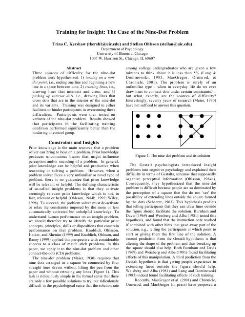
Training for Insight: The Case of the Nine-Dot Problem Trina C. Kershaw (tkersh1@) and Stellan Ohlsson (stellan@)Department of PsychologyUniversity of Illinois at Chicago1007 W. Harrison St., Chicago, IL 60607AbstractThree sources of difficulty for the nine-dot problem were hypothesized: 1) turning on a non-dot point, i.e., ending one line and beginning a new line in a space between dots; 2) crossing lines, i.e., drawing lines that intersect and cross; and 3) picking up interior dots, i.e., drawing lines that cross dots that are in the interior of the nine-dot and its variants. Training was designed to either facilitate or hinder participants in overcoming these difficulties. Participants were then tested on variants of the nine-dot problem. Results showed that participants in the facilitating training condition performed significantly better than the hindering or control group.Constraints and InsightsPrior knowledge is the main resource that a problem solver can bring to bear on a problem. Prior knowledge produces unconscious biases that might influence perception and/or encoding of a problem. In general, prior knowledge can be helpful and productive when reasoning or solving a problem. However, when a problem solver faces a very unfamiliar or novel type of problem, there is no guarantee that prior knowledge will be relevant or helpful. The defining characteristic of so-called insight problems is that they activate seemingly relevant prior knowledge which is not, in fact, relevant or helpful (Ohlsson, 1984b, 1992; Wiley, 1998). To succeed, the problem solver must de-activate or relax the constraints imposed by the more or less automatically activated but unhelpful knowledge. To understand human performance on an insight problem, we should therefore try to identify the particular prior concepts, principles, skills or dispositions that constrain performance on that problem. Knoblich, Ohlsson, Haider, and Rhenius (1999) and Knoblich, Ohlsson, and Raney (1999) applied this perspective with considerable success to a class of match stick problems. In this paper, we apply it to the nine-dot problem and other connect-the-dots (CD) problems.The nine-dot problem (Maier, 1930) requires that nine dots arranged in a square be connected by four straight lines drawn without lifting the pen from the paper and without retracing any lines (Figure 1). This task is ridiculously simple in the formal sense that there are only a few possible solutions to try, but ridiculously difficult in the psychological sense that the solution rate among college undergraduates who are given a few minutes to think about it is less than 5% (Lung & Dominowski, 1985; MacGregor, Ormerod, & Chronicle, 2001). The problem is surely of an unfamiliar type – when in everyday life do we ever draw lines to connect dots under certain constraints? –but what, exactly, are the sources of difficulty? Interestingly, seventy years of research (Maier, 1930) have not sufficed to answer this question.Figure 1: The nine-dot problem and its solution The Gestalt psychologists introduced insight problems into cognitive psychology and explained their difficulty in terms of Gestalts, schemas that supposedly organize perceptual information (Ohlsson, 1984a). Consequently, they hypothesized that the nine-dot problem is difficult because people are so dominated by the perception of a square that the do not 'see' the possibility of extending lines outside the square formed by the dots (Scheerer, 1963). This hypothesis predicts that telling participants that they can draw lines outside the figure should facilitate the solution. Burnham and Davis (1969) and Weisberg and Alba (1981) tested this hypothesis, and found that the instruction only worked if combined with other hints that gave away part of the solution, e.g., telling the participants at which point to start or giving them the first line of the solution. A second prediction from the Gestalt hypothesis is that altering the shape of the problem and thus breaking up the square should also help. Both Burnham and Davis (1969) and Weisberg and Alba (1981) found facilitating effects of this manipulation. A third prediction from the Gestalt hypothesis is that giving people experience in extending lines outside the figure should help. Weisberg and Alba (1981) and Lung and Dominowski (1985) indeed found facilitating effects of such training.Recently, MacGregor et al. (2001) and Chronicle, Ormerod, and MacGregor (in press) have proposedatheory that attempts to predict quantitative differences in solution rates for different CD problems. Their explanation is based on four principles: (a) People always draw their next line so as to go through as many dots as possible. (b) People judge the value of a line as a function of how many dots it picks up in relation to how many dots are left and how many lines they have left to draw. (c) People look ahead 1, 2, 3 or at most 4 steps when deciding which line to draw next. (d) When lookahead indicates that every possible line from the current dot will end in a situation where the next line does not provide sufficient progress, they consider, with some probability, lines that go outside the figure formed by the dots.This theory successfully predicts the differences in solution rates between different several different CD problems. It provides a more detailed description of why people get stuck than any previous theory – their lookahead is not deep enough to reveal that the solution path they are trying will dead end eventually – but the basic explanation for the difficulty is similar to that of previous theories: people consider lines within the shape formed by the dots before they consider lines that go outside the figure.However, if this is true of variants of the nine-dot problems that do not form squares or any other 'good figure', then the Gestalt explanation for why people do not go outside the figure no longer holds. So what is the difficulty?By analyzing pilot data and inspecting MacGregor et al.’s (2001) solution rates for the different nine-dot variants, we hypothesize that "hesitating to go outside the figure formed by the dots" is the wrong formulation of the constraint operating in this type of problem. Instead, we propose that people are disposed to turn on a dot, as opposed to turn on a point on the paper where there is no dot (a non-dot point). This constraint overlaps in meaning with the stay-within-the-figure constraint, so it explains the success of the training provided by Lung and Dominowski (1985). At the same time, this formulation is different enough to explain why telling people that they can go outside the figure does not help; they do not hesitate to extend lines outside the figure, but they do not want to turn on a non-dot point. As a secondary constraint, we hypothesize that people hesitate to cross lines, having a strong disposition towards thinking of the four lines they are supposed to draw as forming a closed outline. As a consequence, they do not see how to pick up the dots in the interior of the figure, an operation that requires crossing lines in many CD problems.In the present study, we tested this hypothesis by both comparing problems that did and did not require turns on non-dot points and by attempting to facilitate the solution via training. As a novel methodological feature, we also tried to hinder the solution with training intended to strengthen the inappropriate constraints.MethodParticipantsParticipants were 90 undergraduates (30 in each training group: facilitating, hindering, and no training) from UIC’s Participant Pool. No demographic data were collected about the participants.MaterialsThe training exercises were designed by the first author. Facilitating Training The facilitating training was designed to eliminate the difficulties that participants were thought to face when solving the nine-dot problem. Twelve training exercises were designed, each with similar instructions to the nine-dot problem (Connect all of these dots using ___ straight lines without lifting your pen from the page and without retracing any lines). Each exercise required a different number of lines to connect the dots.Six of the training exercises required participants to cross lines and pick up interior dots (Figure 2), and the other six could only be solved by turning on a non-dot point (Figure 3). Each training exercise was presented on its own page. The dots were filled circles that were .5 cm in diameter, and the centers of each dot were approximately 3.75 cm apart.Figure 2: Facilitating Training Exercise and its Solution: Crossing Lines and Picking up Interior Dots Hindering Training The hindering training consisted of 12 exercises that were solved by drawing lines that always turned on a dot and never crossed another line (Figure 4). As in the facilitating training, participants were instructed with similar directions to the nine-dot problem (Connect all of these dots using ___ straight lines without lifting your pen from the page and without retracing any lines). Again, each exercise required a different number of lines to connect the dots.Thehindering training was constructed just as the facilitating training, with the dots, or filled circles, being .5 cm in diameter and the centers of each dot being approximately 3.75 cm apart.Figure 3: Facilitating Training Exercise and itsSolution: Turning on a Non-Dot PointNine-Dot Variants The three insight and three non-insight versions of the nine-dot problem that were used had been designed by MacGregor et al. (2001). The insight problems required participants to turn on a non-dot point (Figure 5), while the non-insight problems were the insight problems with an added dot, which excused participants from having to turn on a non-dot point (Figure 6). Each problem was presented on its own page. The dots were filled circles that were 1 cm in diameter. The center of each dot was approximately 3.75 cm apart.Figure 4: Hindering Training Exercise and its Solution ProcedureParticipants were seen in groups of 2-10. Each session lasted from 40 minutes to an hour. All test materials were contained in a booklet.Training Phase Participants in both the facilitating and hindering training conditions were given the same directions for the training exercises. The instructions explained that they would be connecting dots using the number of lines specified on each page without lifting their pens from the page or retracing any lines. They were also told to start at the dot marked with a star for each group. The purpose of giving participants a set starting point was to make sure that there was a single solution for each training exercise.Participants had one minute to work on each training exercise. Time was kept by the experimenter. Participants in the no training (control) group did not complete the training exercises and instead began with the problems.Figure 5: Nine-Dot Variant: Insight VersionFigure 6: Nine-Dot Variant – Non-Insight Version Problem-Solving Phase.After completing the training, participants began the problem-solving section of the booklet. Participants were instructed that they would have four minutes to connect all the dots in the figure using four straight lines without lifting their pens from the page and without retracing any lines. For each problem, there was a practice sheet followed by a second identical sheet with the problem on it. Participants were instructed to try the problem as many times as they wanted to on the practice sheet. When they thought they had come up with a solution, they were to record the time out of the four minutes that had passed, using a large clock at the front of theroom.The participants then were to turn the page and redraw their final solutions on the clean page.The order of problems was the same for all participants. The first problem was an insight problem, the second was a non-insight problem, the third was an insight problem, and so on. Each insight problem was followed by its non-insight version. The first insight problem was of principal interest in comparing the effect of the training manipulations. The other problems were included to obtain baseline solving rates for various problem types, and to compare solving rates in the UIC participant population to the solving rates obtained by MacGregor et al. (2001).ResultsThe results focus on the first insight problem (see Figure 5).Group AnalysisA 3 x 2 chi-square analysis was conducted for the first insight problem. The independent variable was the type of training: facilitating, hindering, or no training. The dependent variable was whether or not a participant had solved the first insight problem. Nineteen participants (63%) in the facilitating group solved the first insight problem, eight (27%) in the hindering group solved, and 11 (37%) in the no training group solved. The chi-square was significant, χ2(2, N = 90) = 8.836, p < .05. Post-hoc comparisons showed significant differences between the facilitating group and the hindering group,χ2(1, N = 60) = 8.148, p < .05, and between the facilitating group and the no training group, χ2(1, N = 60) = 4.267, p < .05, but not between the hindering group and the no training group, χ2(1, N = 60) = .693, p > .05.A between-groups analysis of variance (ANOVA) was conducted for the average amount of time it took participants in each group to solve the first insight problem. Participants in the facilitating group averaged 116 seconds to solve the first insight problem, the hindering group averaged 188 seconds, and the no training group averaged 185 seconds to solve. The ANOVA was significant, F(2,87) = 5.873, p < .05. Post-hoc Tukey tests revealed significant differences between the facilitating group and the hindering group (p < .05) and the facilitating group and the no training group (p < .05), but not between the hindering group and the no-training group (p > .05).Individual Differences AnalysisAlthough the facilitating group did better on the first insight problem than the other two groups, there was a large amount of variation in solving rate within the facilitating training group. Specifically, not all participants in the facilitating training group completed the training correctly. Participants in the facilitating group were split into two sub-groups based on whether or not they had completed the training correctly. In order to be classified as having completed the training correctly, a participant had to correctly complete over half (six) of the training exercises. If a participant did not correctly complete at least six of the training exercises, then he or she was put into the “did not complete training” group. In the “completed training”group, no participant got more than four training exercises incorrect. In the “did not complete training”group, one participant got six exercises wrong, and the others got seven or more exercises wrong.There were a total of 19 participants in the “completed training” group, 17 (89%) of which solved the first insight problem, and 11 participants in the “did not complete training” group, two (18%) of which solved the first insight problem. A chi-square analysis comparing the performance of the two sub-groups on the first insight problem was significant, χ2(1, N = 30) = 15.248, p < .05.Within each group, there were large differences in the amount of time needed to solve the first insight problem. Participants in the facilitating group who solved the first insight problem needed between 8 and 180 seconds to solve, with the majority of solvers requiring between eight and 109 seconds. The amount of time needed to solve ranged between 15 and 235 seconds in the hindering group, and between 20 and 195 seconds in the no training group.DiscussionThe results show that the problems that did not require turns on non-dot points were easier than those that did, and that the facilitating training improved performance on our CD problems, supporting the idea that the difficulties of the nine-dot problem and of CD problems generally might be some combination of a disposition towards turning on a dot and a disposition to think of the four lines they are supposed to draw as forming an outline and hence not crossing each other.Contrary to expectation, the hindering training did not suppress the solution rate below that of a control group. There are several possible explanations. First, the solution rate was low enough so that attempting to suppress it further encountered a floor effect. Second, it is possible that the constraining dispositions were entrenched enough already so that attempting to entrench them yet further with a brief intervention did not succeed.An interesting finding was that for the facilitating group, the degree to which participants completed the training determined their success in solving the firstinsight problem. It is likely that only the participants in the facilitating group who fully completed the training were able to successfully transfer what they had learned during training to solving the insight problems. This finding shows that despite common difficulties for participants in solving CD problems, there exists individual variation in the degree to which participants can be guided to overcome these difficulties.Where would people acquire the two central dispositions to want to turn on a dot and to draw outlines? The first disposition might stem from yet another Gestalt concept, the difference between figure and ground. The dots on the paper is the figure and the paper is the background and hence not part of what they are working on. The disposition to draw outlines might be grounded in how people draw when they try to make representational drawings; they trace the outline of the object they are trying to represent. Even if plausible sources can be identified for these two constraints, it remains to prove that they are operating in the nine-dot problem itself as well as in the altered versions we used in this study.Another reason that people find the nine-dot and related CD problems difficult is that their prior experience in solving CD problems is based in children’s connect-the-dot puzzles. This experience is irrelevant to the knowledge that is needed to solve the nine-dot problem. Prior knowledge creates unconscious biases that are not always helpful (cf. Ohlsson, 1984b, 1992; Wiley, 1998). The presentation of a problem can interact with prior knowledge, thus resulting in an incorrect and unhelpful encoding of the problem.What is of most interest in studies on CD problems is to comprehend how people can get stuck on such trivial problems. To understand how the human mind works, we must understand unhelpful interactions between problems and prior knowledge, the impasses that result, and how people overcome those impasses by relaxing the inappropriate constraints. Insight problems are tools with which to study these processes.ReferencesBurnham, C.A., & Davis, K.G. (1969). The nine-dot problem: Beyond perceptual organization. Psychonomic Science, 17(6), 321-323.Chronicle, E.P., Ormerod, T.C., & MacGregor, J.N. (in press). When insight just won’t come: The failure of visual cues in the nine-dot problem. Quarterly Journal of Experimental Psychology.Knoblich, G., Ohlsson, S., Haider, H., & Rhenius, D. (1999). Constraint relaxation and chunk decomposition in insight problem solving. Journal of Experimental Psychology: Learning, Memory, and Cognition, 25, 1534-1555.Knoblich, G., Ohlsson, S., & Raney, G. (1999). Resolving impasses in problem solving: An eye movement study. In M. Hahn and S. Stoness (Eds.), Proceedings of the Twenty-First Annual Meeting of the Cognitive Science Society (pp. 276-281). Mahwah, NJ: Erlbaum.Lung, C.T., & Dominowski, R.L. (1985). Effects of strategy instructions and practice on nine-dot problem solving. Journal of Experimental Psychology: Learning, Memory, and Cognition, 11(4), 804-811.MacGregor, J.N., Ormerod, T.C., & Chronicle, E.P. (2001). Information-processing and insight: A process model of performance on the nine-dot and related problems. Journal of Experimental Psychology: Learning, Memory, and Cognition,27(1), 176-201.Maier, N.R.F. (1930). Reasoning in humans: I. On direction. Journal of Comparative Psychology, 10, 115-143.Ohlsson, S. (1984a). Restructuring revisited I: Summary and critique of the Gestalt theory of problem solving. Scandinavian Journal of Psychology, 25, 65-78.Ohlsson, S. (1984b). Restructuring revisited II: An information processing theory of restructuring and insight. Scandinavian Journal of Psychology, 25,117-129.Ohlsson, S. (1992). Information processing explanations of insight and related phenomena. In M. Keane and K. Gilhooly (Eds.), Advances in the Psychology of Thinking (Vol.1, pp. 1-44). London: Harvester-Wheatsheaf.Scheerer, M. (1963) Problem solving. Scientific American, 208(4), 118-128.Weisberg, R.W., & Alba, J.W. (1981). An examination of the alleged role of “fixation” in the solution of several “insight” problems. Journal of Experimental Psychology: General, 110(2), 169-192.Wiley, J. (1998). Expertise as mental set: The effects of domain knowledge on creative problem solving. Memory & Cognition, 26(4), 16-730.。
Using the Fractal Dimension to Cluster Datasets Paper 145

George Mason University Information and Software Engineering Department Fairfax, VA 22303
dbarbara,pchen @
Daniel Barbar a
Ping Chen
October 19, 1999
Paper 145
Clustering is a widely used knowledge discovery technique. It helps uncovering structures in data that were not previously known. Clustering of large datasets has received a lot of attention in recent years. However, clustering is a still a challenging task since many published algorithms fail to do well in scaling with the size of the dataset and the number of dimensions that describe the points, or in nding arbitrary shapes of clusters, or dealing e ectively with the presence of noise. In this paper, we present a new clustering algorithm, based in the fractal properties of the datasets. The new algorithm, which we call Fractal Clustering FC places points incrementally in the cluster for which the change in the fractal dimension after adding the point is the least. This is a very natural way of clustering points, since points in the same cluster have a great degree of self-similarity among them and much less self-similarity with respect to points in other clusters. FC requires one scan of the data, is suspendable at will, providing the best answer possible at that point, and is incremental. We show via experiments that FC e ectively deals with large datasets, high-dimensionality and noise and is capable of recognizing clusters of arbitrary shape.
PROEFSCHRIFT

een wetenschappelijke proeve op het gebied van de Natuurwetenschappen, Wiskunde en Informatica
CONTENTS
1. General introduction ....................................................................................................... 3 2. Introduction to clustering multi-spectral images: a tutorial ...................................... 9 2.1 Introduction.............................................................................................................. 10 2.2 Problems for clustering multivariate images ........................................................... 11 2.3 Example images ....................................................................................................... 12 2.4 Similarity Measures ...
- 1、下载文档前请自行甄别文档内容的完整性,平台不提供额外的编辑、内容补充、找答案等附加服务。
- 2、"仅部分预览"的文档,不可在线预览部分如存在完整性等问题,可反馈申请退款(可完整预览的文档不适用该条件!)。
- 3、如文档侵犯您的权益,请联系客服反馈,我们会尽快为您处理(人工客服工作时间:9:00-18:30)。
1
Introduction
Most approaches to semi-supervised learning (SSL) see the problem from one of two (dual) perspectives: supervised classification with additional unlabelled data (see [20] for a recent survey); clustering with prior information or constraints (e.g., [4, 10, 11, 15, 17]). The second perspective, usually termed semi-supervised clustering (SSC), is usually adopted when labels are totaly absent, but there are (usually pair-wise) relations that one wishes to enforce or encourage. Most SSC techniques work by incorporating the constrains (or prior) into classical algorithms such as K-means or EM for mixtures. The semi-supervision may be hard (i.e., grouping constraints [15, 17]), or have the form of a prior under which probabilistic clustering is performed [4, 11]. The later is clearly the most natural formulation for cases where one wishes to encourage, not enforce, certain relations; an obvious example is image segmentation, seen as clustering under a spatial prior, where neighboring sites should be encouraged, but not constrained, to belong to the same cluster/segment. However, the previous EM-type algorithms for this class of methods have a major drawback: the presence of the prior makes the E-step non-trivial, forcing the use of expensive Gibbs sampling [11] or suboptimal methods such as the iterated conditional modes algorithm [4]. In this paper, we introduce a new approach to mixture-based SSC, leading to a simple, fully deterministic, generalized EM (GEM) algorithm. The keystone is the formulation of SSC as a penalized logistic regression problem, where the labels are only indirectly observed. The linearity of the resulting complete log-likelihood, w.r.t. the missing group labels, underlies the simplicity of the resulting GEM algorithm. When applied to image segmentation, our method allows using spatial priors which are typical of image estimation problems (e.g., restoration/denoising), such as Gaussian
fields or wavelet-based priors. Under these priors, the M-step of our GEM algorithm reduces to a simple image denoising procedure, for which there are several extremely efficient algorithms.
Dong Seon Cheng, Vittorio Murino Vision, Image Processing, and Sound Laboratory Dipartimento di Informatica University of Verona Italy cheng@sci.univr.it, vittorio.murino@univr.it
Abstract
This paper proposes a new approach to model-based clustering under prior knowledge. The proposed formulation can be interpreted from two different angles: as penalized logistic regression, where the class labels are only indirectly observed (via the probability density of each class); as finite mixture learning under a grouping prior. To estimate the parameters of the proposed model, we derive a (generalized) EM algorithm with a closed-form E-step, in contrast with other recent approaches to semi-supervised probabilistic clustering which require Gibbs sampling or suboptimal shortcuts. We show that our approach is ideally suited for image segmentation: it avoids the combinatorial nature Markov random field priors, and opens the door to more sophisticated spatial priors (e.g., wavelet-based) in a simple and computationally efficient way. Finally, we extend our formulation to work in unsupervised, semi-supervised, or discriminative modes.
2
Formulation
We start from the standard formulation of finite mixture models: X = {x1 , ..., xn } is an observed data set, where each xi ∈ I Rd was generated (independently) according to one of a set of K probability (density or mass) functions {p(·|φ(1) ), ..., p(·|φ(K ) )}. In image segmentation, each xi is a pixel value (gray scale, d = 1; color, d = 3) or a vector of local (e.g., texture) features. Associated (1) (K ) with X , there is a hidden label set Y = {y1 , ..., yn }, where yi = [yi , ..., yi ]T ∈ {0, 1}K , with (k ) yi = 1 if and only if xi was generated by source k (the so-called “1-of-K” binary encoding). Thus,
Clustering Under Prior Knowledge with Application to Image Segmentation
M´ ario A. T. Figueiredo Instituto de Telecomunicac ¸o ˜ es Instituto Superior T´ ecnico Technical University of Lisbon Portugal mario.figueiredo@lx.it.pt
K n K
p (X |Y , φ ) =
k=1 i: yi
(k)
p(xi |φ
=
(k )
)=
i=1 k=1
p(xi |φ
(k )
)
yi
(k)
,
(1)
where φ = (φ(1) , ..., φ(K ) ) is the set of parameters of the generative models of classes. In standard mixture models, all the yi are assumed to be independent and identically distributed samples following a multinomial distribution with probabilities {η (1) , ..., η (K ) }, i.e., P (Y ) = (k) (k ) yi ) . This is the part of standard mixture models that has to be modified in order to i k (η insert grouping constraints [15] or a grouping prior p(Y ) [4, 11]. However, this prior destroys the simplicity of the standard E-step for finite mixtures, which is critically based on the independence assumption. We follow a different route to avoid that roadblock. Let the hidden labels Y = {y1 , ..., yn } depend on a new set of variables Z = {z1 , ..., zn }, where (1) (K ) each zi = [zi , ..., zi ]T ∈ I RK , following a multinomial logistic model [5]: