A new pathotype characterization of Daxing and Huangyuan populations of cereal cyst nemato

合集下载

智能计算简介

中被完全省去，在进化策略中与自适应结合在一起使用非常性，而从进化策略的角度看，选择是完全确定的，没有合理的根据表明随机选择原则的重要性；
进化规划和进化策略确定地把某些个体排除在被选择复制之外，而标准遗传算法一般对每个个体都指定一个非零选择概率。
智能计算
智能计算
计算智能是以数据为基础，通过训练建立联系，进行问题求解，特点是：
1、以分布式方式存储信息 2、以并行方式处理信息 3、具有自组织、自学习能力 4、计算智能适用于于解决那些难以建立确定性
数学／逻辑模型，或不存在可形式化模型的问题．
智能计算
计算智能以连接主义的思想为基础，有众多发展方向。
遗传算法的基础：孟德尔遗传学
在孟德尔遗传学中，基因型被详细模型化，而表型和环境被忽略。
简单起见，假设一个基因具有n 等位基因a1,…,an。二倍基因型以元组(ai,aj)为特征。我们定义 pij 为总群体中基因型(ai,aj) 的频度。假设基因型与表型相等。质量函数给每个表型赋值。
q(ai,aj) = qij qij 可以被解释为出生率减去死亡率
遗传算法与自然进化的比较
自然界
染色体基因等位基因(allele) 染色体位置(locus) 基因型(genotype) 表型(phenotype)
遗传算法
字符串字符,特征
特征值字符串位置
结构参数集,译码结构
新达尔文进化理论的主要论点
1) 个体是基本的选择目标; 2) 随机过程在进化中起重大作用, 遗传变异大部
分是偶然现象; 3) 基因型变异大部分是重组的产物, 部分是突变; 4) 逐渐进化可能与表型不连续有关; 5) 不是所有表型变化都是自然选择的必然结果; 6) 进化是在适应中变化的, 形式多样, 不仅是基因

链格孢属真菌（Alternaria）属有丝分裂孢子真菌类群丝孢纲丝b...b-YNSTC

链格孢属真菌(Alternaria)属有丝分裂孢子真菌类群丝孢纲丝孢目，是半知菌暗色丝孢菌中一类非常常见的真菌。

链格孢属真菌是引起植物病害的重要真菌类群之一。

大部分链格孢属真菌寄生于不同种植物，特别是农作物，常引起包括玉米、小麦、马铃薯、苹果和番茄等几十种农作物的病害，而给农业造成重大经济损失。

有些链格孢属真菌是人和动物的条件致病菌，常引起多种疾病。

链格孢属真菌产生许多有毒代谢产物，包括腾毒素(tentoxin) ，链格孢毒素(altertoxins)，细交链孢菌酮酸(tenuazonic acid)，交链孢霉烯(altenuene)和交链孢酚(alternariol)等，其中有些毒素是其作用于植物的主要致病因子，通过毒素的作用不仅使植物产生症状，造成危害，而且人和动物摄入被污染的食品或饲料后可导致慢性或急性中毒。

有些毒素可用作除草剂和杀菌剂等，是有应用潜力的生物资源(Barkai-Golan, 2008)。

腾毒素是由一些链格孢属真菌产生的一个天然环四肽。

这个属的链格孢(A. alternata)，柑桔链格孢(A. citri) ，长柄链格孢(A. longipes) ，苹果链格孢(A. mali) ，葱链格孢(A. porri)和细链格孢(A. tenuis)的一些菌株已被报道产生腾毒素(Meyer, 1971; Liebermann, 1983; Kono, 1986; Suemitsu, 1990)。

从腐烂的西红柿和浓缩苹果汁中都检测到被链格孢属真菌污染而产生的腾毒素(Andersen, 2004; 何强，2010)。

腾毒素的化学结构是[cyclo-(L-MeAla-L-Leu-MePhe*(Z)∆+-Gly)] (Meyer, 1971)。

腾毒素的主要生物活性是选择性抑制一些高等植物叶绿体F1-ATP酶活性而导致植物萎黄病(Steele, 1976)。

其抑制机理是低浓度下抑制叶绿体F1-ATP酶中ATP水解和合成(Steele, 1976)，因此常用于研究F1-ATP酶的反应机制(Pavlova, 2004; Meiss, 2008)。

Anytime包将任何类型的输入转换为'POSIXct'或'Date'对象说明书

Package‘anytime’October12,2022Type PackageTitle Anything to'POSIXct'or'Date'ConverterVersion0.3.9Date2020-08-26Author Dirk EddelbuettelMaintainer Dirk Eddelbuettel<**************>Description Convert input in any one of character,integer,numeric,factor,or ordered type into'POSIXct'(or'Date')objects,using one of a number ofpredeﬁned formats,and relying on Boost facilities for date and time parsing.URL /code/anytime.htmlBugReports https:///eddelbuettel/anytime/issuesLicense GPL(>=2)Encoding UTF-8Depends R(>=3.2.0)Imports Rcpp(>=0.12.9)LinkingTo Rcpp(>=0.12.9),BHSuggests tinytest(>=1.0.0),gettzRoxygenNote6.0.1NeedsCompilation yesRepository CRANDate/Publication2020-08-2711:40:21UTCR topics documented:anytime-package (2)anytime (3)assertDate (7)getFormats (8)iso8601 (9)Index1112anytime-package anytime-package Anything to’POSIXct’or’Date’ConverterDescriptionConvert input in any one of character,integer,numeric,factor,or ordered type into’POSIXct’(or ’Date’)objects,using one of a number of predeﬁned formats,and relying on Boost facilities for date and time parsing.DetailsR excels at computing with dates,and ing typed representation for your data is highly recommended not only because of the functionality offered but also because of the added safety stemming from proper representation.But there is a small nuisance cost in interactive work as well as in programming.How often have we told as.POSIXct()that the origin is(of course)the epoch.Do we really have to say it again?Similarly,when parsing dates that are somewhat in YYYYMMDD format,do we really need to bother converting from integer or numeric or character or factor or ordered with one of dozen separators and/or month forms:YYYY-MM-DD,YYYY/MM/DD,YYYYMMDD,YYYY-mon-DD and so on?So there may have been a need for a general purpose converter returning a proper POSIXct(or Date)object no matter the input(provided it was somewhat parseable).anytime()tries to be that function.The actual conversion is done by a combination of Boost lexical_cast to go from(almost)anything to string representation which is then parsed by Boost Date_Time.An alternate method using the corresponding R functions is also available as a fallback.Conversion is done by looping over aﬁxed set of formats until a matching one is found,or returning an error if none is found.The current set of conversion formulae is accessible in the source code, and can now also be accessed in R via getFormats().Formats can be added and removed via the addFormats()and removeFormats{}functions.Details on the Boost date format symbols are provided by the Boost date_time documentation and similar(but not identical)to what strftime uses.Author(s)Dirk EddelbuettelReferencesBoost date_time:https:///doc/libs/1_70_0/doc/html/date_time.htmlFormats used:https:///eddelbuettel/anytime/blob/master/src/anytime.cpp# L43-L106Boost format documentation:https:///doc/libs/1_61_0/doc/html/date_time/ date_time_io.html#date_time.format_flagsExamplesSys.setenv(TZ=anytime:::getTZ())##helper function to try to get TZoptions(digits.secs=6)##for fractional seconds belowlibrary(anytime)##load package,caches TZ information##integeranydate(20160101L+0:2)##numericanydate(20160101+0:2)##factoranydate(as.factor(20160101+0:2))##orderedanydate(as.ordered(20160101+0:2))##Dates:Characteranydate(as.character(20160101+0:2))##Dates:alternate formatsanydate(c("20160101","2016/01/02","2016-01-03"))##Datetime:ISO with/without fractional secondsanytime(c("2016-01-0110:11:12","2016-01-0110:11:12.345678"))##Datetime:ISO alternate(?)with T separatoranytime(c("20160101T101112","20160101T101112.345678"))##Short month %b (and full month is supported too)anytime(c("2016-Sep-0110:11:12","Sep/01/201610:11:12","Sep-01-201610:11:12"))##Datetime:Mixed format(cf https:///questions/39259184)anytime(c("Thu Sep0110:11:122016","Thu Sep0110:11:12.3456782016"))anytime Parse POSIXct or Date objects from input dataDescriptionThese function use the Boost Date_Time library to parse datetimes(and dates)from strings,inte-gers,factors or even numeric values(which are cast to strings internally).They return a vector of POSIXct objects(or Date objects in the case of anydate).POSIXct objects represent dates and time as(possibly fractional)seconds since the‘epoch’of January1,1970.A timezone can be set, if none is supplied‘UTC’is set.Usageanytime(x,tz=getTZ(),asUTC=FALSE,useR=getOption("anytimeUseRConversions",FALSE),oldHeuristic=getOption("anytimeOldHeuristic",FALSE),calcUnique=FALSE)anydate(x,tz=getTZ(),asUTC=FALSE,useR=getOption("anytimeUseRConversions",FALSE),calcUnique=FALSE)utctime(x,tz=getTZ(),useR=getOption("anytimeUseRConversions",FALSE),oldHeuristic=getOption("anytimeOldHeuristic",FALSE),calcUnique=FALSE)utcdate(x,tz=getTZ(),useR=getOption("anytimeUseRConversions",FALSE),calcUnique=FALSE)Argumentsx A vector of type character,integer or numeric with date(time)expressions to be parsed and converted.tz A string with the timezone,defaults to the result of the(internal)getTZ function if unset.The getTZ function returns the timezone values stored in local packageenvironment,and set at package load time.Also note that this argument appliesto the output:the returned object will have this timezone set.The timezone isnot used for the parsing which will always be to localtime,or to UTC is theasUTC variable is set(as it is in the related functions utctime and utcdate).So one can think of the argument as‘shift parsed time object to this timezone’.This is similar to what format()in base R does,but our return value is still aPOSIXt object instead of a character value.asUTC A logical value indicating if parsing should be to UTC;default is false implying localtime.useR A logical value indicating if conversion should be done via code from R(via Rcpp::Function)instead of the default Boost routines.The default value is thevalue of the option anytimeUseRConversions with a fallback of FALSE if theoption is unset.In other words,this will be false by default but can be set to truevia an option.oldHeuristic A logical value to enable behaviour as in version0.2.2or earlier:interpret a numeric or integer value that could be seen as a YYYYMMDD as a date.If thedefault value FALSE is seen,then numeric values are used as offsets dates(inanydate or utcdate),and as second offsets for datetimes otherwise.A defaultvalue can also be set via the anytimeOldHeuristic option.calcUnique A logical value with a default value of FALSE that tells the function to perform the anytime()or anydate()calculation only once for each unique value inthe x vector.It results in no difference in inputs or outputs,but can result in asigniﬁcant speed increases for long vectors where each timestamp appears morethan once.However,it will result in a slight slow down for input vectors whereeach timestamp appears only once.DetailsA number ofﬁxed formats are tried in succession.These include the standard ISO format‘YYYY-MM-DD HH:MM:SS’as well as different local variants including several forms popular in the United States.Two-digits years and clearly ambigous formats such as‘03/04/05’are ignored.In the case of parsing failure a NA value is returned.Fractional seconds are supported as well.As R itself only supports microseconds,the Boost compile-time option for nano-second resolution has not been enabled.ValueA vector of POSIXct elements,or,in the case of anydate,a vector of Date objects.NotesBy default,the(internal)conversion to(fractional)seconds since the epoch is relative to the locatime of this system,and therefore not completely independent of the settings of the local system.This is to strike a balance between ease of use and functionality.A more-full featured conversion could be possibly be added with support for arbitrary reference times,but this is(at least)currently outside the scope of this package.See the RcppCCTZ package which offers some timezone-shifting and differencing functionality.As of version0.0.5one can also parse relative to UTC avoiding the localtime issue,Times and timezones can be tricky.This package offers a heuristic approach,it is likely that some input formats may not be parsed,or worse,be parsed incorrectly.This is not quite a Bobby Tables situation but care must always be taken with user-supplied input.The Boost Date_Time library cannot parse single digit months or days.So while‘2016/09/02’works(as expected),‘2016/9/2’will not.Other non-standard formats may also fail.There is a known issue(discussed at length in issue ticket5)where Australian times are off by an hour.This seems to affect only Windows,not Linux.When given a vector,R will coerce it to the type of theﬁrst element.Should that be NA,surprising things can happen:c(NA,Sys.Date())forces both values to numeric and the date will not be parsed correctly(as its integer value becomes numeric before our code sees it).On the other hand, c(Sys.Date(),NA)works as expected parsing as type Date with one missing value.See issue ticket11for more.Another known issue concerns conversion when the timezone is set to‘Europe/London’,see GitHub issue tickets36.51.59.and86.As pointed out in the comment in that last one,the Sys.timezone manual page suggests several alternatives to using‘Europe/London’such as‘GB’.Yet another known issue arises on Windows due to designs in the Boost library.While we can set the TZ library variable,Boost actually does not consult it but rather relies only on the(Windows) tool tzutil.This means that default behaviour should be as expected:dates and/or times are parsed to the local settings.But testing different TZ values(or more precisely,changes via the(unexported) helper function setTZ function as we cache TZ)will only inﬂuence the behaviour on Unix or Unix-alike operating systems and not on Windows.See the discussion at issue ticket96for more.In short,the recommendation for Windows user is to also set useR=TRUE when setting a timezone argument.Operating System ImpactOn Windows systems,accessing the isdstﬂag on dates or times before January1,1970,can leadto a crash.Therefore,the lookup of this value has been disabled for those dates and times,whichcould therefore be off by an hour(the common value that needs to be corrected).It should not affectdates,but may affect datetime objects.Old HeuristicUp until version0.2.2,numeric input smaller than an internal cutoff value was interpreted as adate,even if anytime()was called.While convenient,it is also inconsistent as we otherwise takenumeric values to be offsets to the epoch.Newer version are consistent:for anydate,a value istaken as date offset relative to the epoch(of January1,1970).For anytime,it is taken as secondsoffset.So anytime(60)is one minute past the epoch,and anydate(60)is sixty days past it.The old behaviour can be enabled by setting the oldHeuristic argument to anytime(and utctime)to TRUE.Additionally,the default value can be set via getOption("anytimeOldHeuristic")which can be set to TRUE in startupﬁle.Note that all other inputs such character,factor or ordered are notaffected.Author(s)Dirk EddelbuettelReferencesThis StackOverﬂow answer provided the initial idea:https:///a/3787188/ 143305.See Alsoanytime-packageExamples##See the source code for a full list of formats,and the##or the reference in help( anytime-package )for detailstimes<-c("2004-03-2112:45:33.123456","2004/03/2112:45:33.123456","20040321124533.123456","03/21/200412:45:33.123456","03-21-200412:45:33.123456","2004-03-21","20040321","03/21/2004","03-21-2004","20010101")anytime(times)anydate(times)utctime(times)utcdate(times)assertDate7 ##show effect of tz argumentanytime("2001-02-0304:05:06")##adjust parsed time to given TZ argumentanytime("2001-02-0304:05:06",tz="America/Los_Angeles")##somewhat equvalent base R functionalityformat(anytime("2001-02-0304:05:06"),tz="America/Los_Angeles")assertDate Convert to Date(or POSIXct)and assert successful conversionDescriptionConverts its input to type Date(or POSIXct),and asserts that the content is in fact of suitable type by checking for remaining NAUsageassertDate(x)assertTime(x)Argumentsx An input object suitable for anydate or anytimeDetailsNote that these functions just check for NA and cannot check for semantic correctness.ValueA vector of Date or POSIXct objects.As a side effect,an error will be thrown in any of the inputwas not convertible.Author(s)Dirk EddelbuettelExamplesassertDate(c("2001/02/03","2001-02-03","20010203"))assertTime(c("2001/02/0304:05:06","2001-02-0304:05:06","20010203040506"))8getFormats getFormats Functions to retrieve,set or remove formats used for parsing dates.DescriptionThe time and date parsing and conversion relies on trying a(given andﬁxed)number of timeformats.The format used is the one employed by the underlying implementation of the Boost date_time library.UsagegetFormats()addFormats(fmt)removeFormats(fmt)Argumentsfmt A vector of character values in the form understood by Boost date_timeValueNothing in the case of addFormats;a character vector of formats in the case of getFormatsAuthor(s)Dirk EddelbuettelSee Alsoanytime-package and references thereinExamplesgetFormats()addFormats(c("%d%b%y",#two-digit date[not recommended],textual month"%a%b%d%Y"))#weekday weeknumber four-digit yearremoveFormats("%d%b%y")#remove firstiso8601Format a Datetime object:ISO8601,RFC2822or RFC3339DescriptionISO8601,RFC2822and RFC3339are a standards for date and time representation covering the formatting of date and time(with or without possible fractional seconds)and timezone information. Usageiso8601(pt)rfc2822(pt)rfc3339(pt)yyyymmdd(pt)Argumentspt A POSIXt Datetime or a Date objectValueA character object formatted according to ISO8601,RFC2822or RFC3339ISO8601ISO8601is described in some detail in https:///wiki/ISO_8601and covers multiple date and time formats.Here,we interpret it more narrowly focussing on a single format each for datetimes and dates.We return datetime object formatted as‘2016-09-01T10:11:12’and date object as‘2016-09-01’.If the option anytimeOldISO8601format is set to TRUE,then the previous format(with a space instead of‘T’to separate date and time)is used.RFC2822RFC2822is described in some detail in https:///rfc/rfc2822.txt and https: ///wiki/Email#Internet_Message_Format.The Date and Time formating cover only a subset of the speciﬁcation in that RFC.Here,we use it to provide a single format each for datetimes and dates.We return datetime object formatted as‘Thu,01Sep201610:11:12.123456-0500’and date object as‘Thu,01Sep2016’.RFC3339RFC3339is described in some detail in https:///html/rfc3339It reﬁnes both earlier standards.Here,we use it to format datetimes and dates as single and compact strings.We return datetime object formatted as‘2016-09-01T10:11:12.123456-0500’and date object as‘2016-09-01’. YYYYMMDDThis is a truly terrible format which needs to die,but refuses to do so.If you are unfortunate enough to be forced to interoperate with code expecting it,you can use this function.But it would be better to take a moment to rewrite such code.Author(s)Dirk EddelbuettelReferenceshttps:///wiki/ISO_8601,https:///rfc/rfc2822.txt,https: ///wiki/Email#Internet_Message_Format,https:///html/ rfc3339Examplesiso8601(anytime("2016-09-0110:11:12.123456"))iso8601(anydate("2016-Sep-01"))rfc2822(anytime("2016-09-0110:11:12.123456"))rfc2822(anydate("2016-Sep-01"))rfc3339(anytime("2016-09-0110:11:12.123456"))rfc3339(anydate("2016-Sep-01"))yyyymmdd(anytime("2016-09-0110:11:12.123456"))yyyymmdd(anydate("2016-Sep-01"))Index∗packageanytime-package,2addFormats(getFormats),8anydate(anytime),3anytime,3anytime-package,2assertDate,7assertTime(assertDate),7getFormats,8iso8601,9removeFormats(getFormats),8rfc2822(iso8601),9rfc3339(iso8601),9strftime,2Sys.timezone,5utcdate,4utcdate(anytime),3utctime,4utctime(anytime),3yyyymmdd(iso8601),911。

字符合集和出现概率构造哈夫曼树

《字符合集和出现概率构造哈夫曼树》一、引言在信息技术领域，字符合集和出现概率构造哈夫曼树是一项重要且基础的概念。

本文将深入探讨字符合集和哈夫曼树的构造过程，并分析字符出现概率对哈夫曼树构造的影响，旨在让读者对此理解更加深入、全面。

二、字符合集和出现概率字符合集是指在某种编码方式下所能使用的字符的总体。

在计算机领域中，字符合集通常指的是能够表示文本、图像、声音等信息的全部字符。

而字符的出现概率则是指在一个文本或数据集中某个字符出现的频率，通常使用概率分布来表示。

在构造哈夫曼树的过程中，首先需要了解字符合集中各个字符的出现概率，因为出现概率越高的字符，在哈夫曼编码中对应的编码长度应该越短，以提高编码效率。

对字符合集中字符出现概率的准确评估对于哈夫曼树的构造至关重要。

三、哈夫曼树的构造步骤1. 根据字符出现概率构造叶子节点：首先根据给定的字符合集以及各字符的出现概率，构造对应的叶子节点。

出现概率较高的字符对应的叶子节点应该在哈夫曼树中拥有较短的路径长度。

2. 构造哈夫曼树的内部节点：在构造叶子节点之后，根据哈夫曼树的构造规则，通过不断合并概率最小的两个节点来构造内部节点，并更新概率信息。

这一过程直到所有节点合并成为一个根节点为止。

3. 确定字符的编码：通过遍历哈夫曼树的路径，确定每个字符对应的编码，从而完成哈夫曼编码的构造。

四、字符出现概率对哈夫曼树的影响字符出现概率对哈夫曼树的构造有着重要的影响。

在实际应用中，如果字符出现概率相差较大，那么对应的编码长度也会存在较大的差异。

合理评估字符出现概率，能够在一定程度上提高哈夫曼编码的效率。

当字符出现概率相近的时候，构造的哈夫曼树将会比较平衡，对应的编码长度也会较为接近，这样能够保证在编码和解码的过程中效率的平衡。

而当字符出现概率差异较大时，哈夫曼树将会不平衡，对应的编码长度也会存在较大的差异，这样就需要根据实际情况来平衡编码的效率和解码的效率。

五、我的观点和理解在我看来，字符合集和出现概率构造哈夫曼树是一项非常重要的基础概念。

PAML操作

PAML软件的一些简单的具体的使用操作1. 首先用Clustal X进行序列比对：要保证：保证核苷酸序列是三的倍数，没有终止密码子，核苷酸序列的第一位是密码子的第一位。

假设序列名为cox1.fas2. 使用DAMBE软件进行转换成PML格式。

打开要换换的文件，然后“file” “save and convert sequence format”，在保存类型中选择“Yang’s PAML”。

那么此时的序列名为“cox1.PML”，这样就可以得到文件“*.PML”，然后就直接把后缀改成“*.nuc”。

那么此时的序列名为“cox1.nuc” 这样就完成了文件格式的转换。

3. 打开PAML软件的文件夹，找到文件名是“bin”的文件夹，打开之后，找到程序“codeml.exe”,把该程序复制到D盘的根目录下。

（这一步并不是必要的，只是要把用到的几个程序放在同一个目录下）4. 在你使用ClustalX进行序列比对的时候，会生成一棵进化树，适用treeview软件可以打开，你需要的是把文件的后缀名改称“*.trees”。

即树的文件名是“cox1.trees”，这就完成了树的格式的转换。

5. 然后再PAML4的文件夹中找到一个后缀是“*.ctl”的文件，把文件名改成“cox1.ctl”，复制到和“codeml.exe”相同的地方。

6. 要对codeml.ctl文件中的各个选项的值进行修改，具体内容如下：seqfile = cox1.nuc 按你自己的文件名进行修改，就可以了， treefile = cox1.treesoutfile = mlc * main result file name ，noisy = 9 * 0,1,2,3,9: how much rubbish on the screen ， verbose = 0 * 0: concise; 1: detailed, 2: too muchrunmode = 0seqtype = 1 * 1:codons; 2:AAs; 3:codons-->AAsCodonFreq = 2 * 0:1/61 each, 1:F1X4, 2:F3X4, 3:codon table clock = 0aaDist = 0 * 0:equal, +:geometric; -:linear,1-6:G1974,Miyata,c,p,v,aaaRatefile = wag.dat * only used for aa seqs withmodel=empirical(_F) *dayhoff.dat,jones.dat,wag.da t,am.dat, or your ownmodel = 0，这是使用的最简单的模型， * models for codons: * 0:one, 1:b, 2:2 or more dN/dS ratios for branches * models for AAs or codon-translated AAs:* 0:poisson, 1:proportional, 2:Empirical, 3:Empirical+F 28 * 6:FromCodon, 7:AAClasses,8:REVaa_0,9:REVaa(nr=189)NSsites = 0 3 1 2 7 8 ，依次选取了6个模型。

毕业小设计

摘要本文所设计的纱线恒张力控制装置以SST89E564RD芯片为其控制核心，硬件部分包含张力测量，张力调节，硬件电路设计及设备产品外形设计等四大模块。

张力控制过程中张力调节模块根据张力测量模块所测得张力数据，数据经过处理后以遗传算法来对PID控制器参数进行自适应调整，并生成控制量改变直流无刷电机转速，从而对纱线中的张力进行控制，此设计解决了纺织过程中纱线张力小和张力变化速度快所带来的纱线张力难以控制的问题。

关键词：纱线张力控制,自适应,遗传算法,PID控制目录1.前言 (1)1.1纱线恒力控制器的背景 (1)1.2 研究的目的及意义 (1)1.3国内外研究现状 (1)1.4课题研究及内容 (2)2.系统分析 (3)2.1纱线张力的产生和作用 (3)2.2纱线张力组成 (3)2.3影响张力波动的因素 (3)2.4张力控制系统方案设计 (3)2.5张力控制系统的测量模块 (3)2.5.1 张力测量模块 (3)2.5.2纱线张力测量模块设计 (4)2.6纱线张力调节模块 (5)2.7 电机选择及控制原理 (6)3.用遗传算法实现纱线张力的PID控制 (7)3.1使用PID进行纱线张力控制的意义 (7)3.2 遗传算法PID控制的引入 (7)3.3 遗传算法基本原理 (7)3.4 基于遗传算法的PID参数优化 (8)3.4.1 基于遗传算法整定PID控制器的参数的步骤 (8)3.4.2 参数编码与解码 (9)3.4.3 初始种群的构建 (10)3.4.4 适应度函数的确定 (10)4 硬件电路设计 (11)4.1 硬件电路功能分析 (11)4.2 A/D转换接口 (11)4.3 ADC0809与单片机接口设计 (12)4.4 直流电机驱动电路 (13)4.4.1 驱动电路的选型 (13)4.4.2 驱动电路接口设计 (14)4.5 人机接口（显示器、按键） (15)5.总体结构及外形设计 (17)6，软件设计 (18)6.1遗传算法PID的实现 (18)6.2 电机驱动程序 (19)6.3 A/D转换程序 (20)7.总结与结论 (22)7.1 研究结论 (22)7.2 工作展望 (22)参考文献 (23)1 前言随着人类生活水平的提高，对衣食住行的要求也随之提高，而衣更具有代表性；人们越来越注重自己的外在表现，尤其是能够体现自己品味和气质的穿着，例如，根据每天的天气或者要见什么人，或去什么地方，来决定穿什么样的衣服；以至于人们对衣物的需求越来越个性化和多样化，这些都是纺织行业需要面对的挑战和机遇。

杨树HDZIP基因家族全基因组研究

573-581．[2]URUO T，YAMAGUCHI-SHINOZAKI K，URAO S，SHINOZAKI K.．An Arabidopsis MYB homolog is induced by dehydration stress and its gene product binds to the conserved MYB recognition sequence[J]．Plant Cell，1993，5(11)：1529-1539．[3]JUNG C，SEO JS，HAN SW，KOO YJ，KIM CH，SONG SI，NALLNL BH，CHOI YD，CHEONG JJ，Overexpression of AtMYB44 Enhances Stomatal Closure to Confer Abiotic Stress Tolerance in Transgenic Arabidopsis[J]．Plant Physiol，2008，146：623-635．[4] DAI XY，XU YY，MA QB，XU WY，Wang T，XUE YB，CHONG K．Overexpression of a R1R2R3MYB gene，OsMYB3R2，increases tolerance to freezing, drought, and salt stress in transgenic Arabidopsis[J]．Plant Physiol，2007，143：1739-1751．[5] PAZ-ARES J，GHOSAL D，WIENAND U，et al．The regulatory c1 locus of Zea mays encodes a protein with homology to myb proto-oncogene products and with structural similarities to transcriptional activators [J]．The EMBO Journal，1987(12)：3553-3558．杨树HD-ZIP基因家族全基因组研究作者：陈雪指导教师：项艳(安徽农业大学林学与园林学院，安徽合肥230036)摘要：同源异型-亮氨酸拉链(HD-ZIP)蛋白是植物所特有的一类转录因子，类属于同源异型盒蛋白家族，它包含一个高度保守的同源异型结构域(HD)，HD羧基末端紧连接着一个亮氨酸拉链(LZ)结构域。

蛋白质PDB文件说明

字符集合只是一些非控制型字符，象空格和结束符，出现在PDB文件记录中。

也就是：abcdefghijklmnopqrstuvwxyzABCDEFGHIJKLMNOPQRSTUVWXYZ1234567890` - = [ ] \ ; ' , . / ~ ! @ # $ % ^ & * ( ) _ + { } | : " < > ?空格和结束符。

结束符根据系统而定，Unix用一行字符，而其他的系统可能就用一个回车来表示。

特殊字符希腊字母就详细的拼写出来。

比如：α, β, γ原子用DOT表示。

右箭头用-->表示。

左箭头用<--表示。

上标用两个等号表示开始和结束。

比如：S＝＝2+＝＝下标用一个等号来表示开始和结束。

比如：F=c=如果等号两边至少有一边有一个空格，那么这个字符就是表示等号。

比如：2 + 4 = 6逗号，冒号和括号用来表示文档中的分界苻，也就是下面几种中的一种：ListSListSpecification ListSpecification如果逗号，冒号或者括号在任何一片文档中使用不是作为分界苻的话，那么肯定有字符被漏掉了。

比如下边例子中第四行的"\"：COMPND MOL_ID: 1;COMPND 2 MOLECULE: GLUTA THIONE SYNTHETASE;COMPND 3 CHAIN: NULL;COMPND 4 SYNONYM: GAMMA-L-GLUTAMYL-L-CYSTEINE\:GL YCINE LIGASECOMPND 5 (ADP-FORMING);COMPND 6 EC: 6.3.2.3;COMPND 7 ENGINEERED: YESCOMPND MOL_ID: 1;COMPND 2 MOLECULE: S-ADENOSYLMETHIONINE SYNTHETASE;COMPND 3 CHAIN: A, B;COMPND 4 SYNONYM: MA T, A TP\:L-METHIONINE S-ADENOSYLTRANSFERASE;COMPND 5 EC: 2.5.1.6;COMPND 6 ENGINEERED: YES;COMPND 7 BIOLOGICAL_UNIT: TETRAMER;COMPND 8 OTHER_DETAILS: TETRAGONAL MODIFICATION数据类型-------------------------------------该部分该部分主要用来描述试验和记录中该大分子的一些基本信息,有以下几种记录:HEADER,OBSLTE,TITTITLE,CA VEA T,COMPND,SOURCE,KEYWDS,EXPDTA,AUTHOR,REVDA T,SPRSDE,JRNL和REMARK部分。

改进的SLTP方法在掌纹识别中的应用

改进的SLTP方法在掌纹识别中的应用彭晏飞;周南;林森【摘要】对掌纹识别进行研究,提出了基于改进的软直方图局部三值模式(SLTP)的掌纹识别方法.该方法先对掌纹训练样本进行能量函数的构造,然后用梯度下降法对能量函数进行优化,得到最佳的模糊隶属度函数,进而对掌纹的特征进行提取,最后用Chi概率统计的相似度度量方法进行匹配识别.在PolyU掌纹数据库和IITD掌纹数据库中进行实验验证,结果表明,在相同的训练样本下,改进的SLTP方法相比于SLTP方法,识别率得到提高.从而证明了该方法的有效性.【期刊名称】《计算机工程与应用》【年(卷),期】2016(052)005【总页数】6页(P179-184)【关键词】掌纹识别;软直方图局部三值模式;梯度下降法;模糊隶属度函数;Chi概率统计【作者】彭晏飞;周南;林森【作者单位】辽宁工程技术大学电子与信息工程学院,辽宁葫芦岛125105;辽宁工程技术大学电子与信息工程学院,辽宁葫芦岛125105;辽宁工程技术大学电子与信息工程学院,辽宁葫芦岛125105【正文语种】中文【中图分类】TP391.41随着科学技术的发展，越来越多的场合需要验证人们合法的身份，因而，个人信息的安全性就显得至关重要，如何建立一个可以自动识别身份的计算机系统成为众多人关注的问题。

生物识别技术[1]以其普遍性、持久性、唯一性、实用性和安全性等优点脱颖而出，如指纹识别[2]、虹膜识别技术[3]等。

然而，掌纹识别以其识别率高、采集设备低廉、用户可接受性好等优点[4]，近年来得到广泛的关注。

掌纹识别主要分为基于线性特征[5]、基于子空间特征[6-7]和基于纹理特征[8]的方法。

线性特征的方法是利用边缘算子和方向模板等对掌纹的褶皱和主线进行提取。

一般情况下，这种方法提取的主线特征比较直观且稳定；子空间方法是通过映射变换，将高维的掌纹数据转换到低维的子空间中，然后再进行处理；纹理的方法主要利用掌纹丰富的纹理信息，提取到图像的特征，这些方法中，纹理特征的方法应用最为普遍。

15个果桑无性系指纹图谱的构建

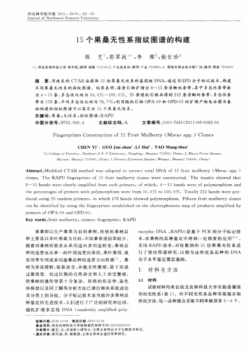
Ｈｕａｘｉｎ，Ｓａａｘ１３０，Ｃｈｉａ；３ＦｏｅｔｙＥｘｔｎｉｎＳａｉｎ，Ｗｅｎｎ，Ｓｈａｘｉ７４０ｈｎｉ７００ｎ．ｒｓｒｅｓｏｔｔｏｉａａｎ１００，Ｃｎｈｉａ）
ＡｂｔａｔＭｏｉｉｄＣＴＡＢｅｈｏａａｐｔｄｔｅｔａｔｏｔｌｓｒｃ：ｄｆｅｍｔｄｗｓｄｏｅｏｘｒｃｔａＤＮＡｏ１ｆｕｉｆ５ｒｔｕｌｒｙ（ｏｒｐｍｂｅｒＭｕｓｓｐ．）
分研磨成粉状；人２ｍＬ离心管中，入预热提取移加液８０ｍＩ，加入Ｊ巯基乙醇（）０ｍＩ匀，５再３一１３混
００１ｔｏ・ＩＥＴＡｐ．）解；入１．０ｌｏ～ＤＨ８０溶加０ｍＩ
（．北农林科技大学林学院，西杨陵７２０；．县林业局，西户县７００；３１西陕１１０２户陕１３０．渭南市林业技术推广站，西渭南７４０）陕１００
摘要：改良的Ｃ用ＴＡＢ法提取１５份果桑无性系的基因组ＤＮＡ，过ＲＤ分子标记技术，建通ＡＰ构
树为异花授粉，易杂交，能无性繁殖，于形成很并易
ｍｏｐｉＤｒｈｃＮＡ，ＡＰ是基于ＰＲ的分子标记技ＲＤ）Ｃ术，桑树的品种鉴定中得到一定程度的应用口］在。采用ＲＤ技术，收集到的１ＡＰ对５份果桑无性系进

《基于多线程技术的水平基因转移事件识别算法研究与平台构建》范文

《基于多线程技术的水平基因转移事件识别算法研究与平台构建》篇一一、引言近年来，随着生物学和计算机科学的交叉发展，基因组学领域的研究取得了显著的进步。

其中，水平基因转移（Horizontal Gene Transfer, HGT）事件作为生物进化过程中的重要现象，对于理解生物多样性和物种演化的机制具有重要意义。

本文旨在研究基于多线程技术的水平基因转移事件识别算法，并构建相应的平台以实现高效、准确的识别。

二、水平基因转移事件概述水平基因转移是指不同生物体之间直接进行的基因交流过程，与传统的垂直遗传方式（即亲代遗传给子代）不同。

这一过程在细菌、病毒、真核生物等生物体中广泛存在，对于生物的适应性和进化具有重要影响。

因此，准确识别水平基因转移事件对于揭示生物进化的奥秘具有重要意义。

三、多线程技术概述多线程技术是一种计算机科学中的并行处理技术，通过在单个程序中同时运行多个独立线程来实现高效的计算和任务处理。

在生物信息学领域，多线程技术可以用于加速大规模数据处理和分析过程，提高计算效率和准确性。

因此，将多线程技术应用于水平基因转移事件的识别具有很大的潜力。

四、基于多线程技术的水平基因转移事件识别算法研究（一）算法设计本文提出的水平基因转移事件识别算法采用多线程技术，通过并行处理大量基因序列数据，加速识别过程。

算法主要包括以下步骤：数据预处理、序列比对、相似性分析、转移事件识别和结果输出。

其中，数据预处理和序列比对采用多线程技术进行并行处理，以提高计算速度。

（二）算法实现算法实现过程中，我们采用了高效的编程语言和工具，如Python、C++等，以及常用的生物信息学软件和数据库。

通过优化算法结构和提高计算效率，实现了快速、准确的水平基因转移事件识别。

五、平台构建（一）平台架构设计平台采用模块化设计，包括数据输入模块、算法处理模块、结果输出模块等。

其中，算法处理模块采用多线程技术进行加速处理。

平台支持多种格式的基因序列数据输入，以及灵活的参数设置和结果输出方式。

Anomaly Detection A Survey(综述)

A modiﬁed version of this technical report will appear in ACM Computing Surveys,September2009. Anomaly Detection:A SurveyVARUN CHANDOLAUniversity of MinnesotaARINDAM BANERJEEUniversity of MinnesotaandVIPIN KUMARUniversity of MinnesotaAnomaly detection is an important problem that has been researched within diverse research areas and application domains.Many anomaly detection techniques have been speciﬁcally developed for certain application domains,while others are more generic.This survey tries to provide a structured and comprehensive overview of the research on anomaly detection.We have grouped existing techniques into diﬀerent categories based on the underlying approach adopted by each technique.For each category we have identiﬁed key assumptions,which are used by the techniques to diﬀerentiate between normal and anomalous behavior.When applying a given technique to a particular domain,these assumptions can be used as guidelines to assess the eﬀectiveness of the technique in that domain.For each category,we provide a basic anomaly detection technique,and then show how the diﬀerent existing techniques in that category are variants of the basic tech-nique.This template provides an easier and succinct understanding of the techniques belonging to each category.Further,for each category,we identify the advantages and disadvantages of the techniques in that category.We also provide a discussion on the computational complexity of the techniques since it is an important issue in real application domains.We hope that this survey will provide a better understanding of the diﬀerent directions in which research has been done on this topic,and how techniques developed in one area can be applied in domains for which they were not intended to begin with.Categories and Subject Descriptors:H.2.8[Database Management]:Database Applications—Data MiningGeneral Terms:AlgorithmsAdditional Key Words and Phrases:Anomaly Detection,Outlier Detection1.INTRODUCTIONAnomaly detection refers to the problem ofﬁnding patterns in data that do not conform to expected behavior.These non-conforming patterns are often referred to as anomalies,outliers,discordant observations,exceptions,aberrations,surprises, peculiarities or contaminants in diﬀerent application domains.Of these,anomalies and outliers are two terms used most commonly in the context of anomaly detection; sometimes interchangeably.Anomaly detectionﬁnds extensive use in a wide variety of applications such as fraud detection for credit cards,insurance or health care, intrusion detection for cyber-security,fault detection in safety critical systems,and military surveillance for enemy activities.The importance of anomaly detection is due to the fact that anomalies in data translate to signiﬁcant(and often critical)actionable information in a wide variety of application domains.For example,an anomalous traﬃc pattern in a computerTo Appear in ACM Computing Surveys,092009,Pages1–72.2·Chandola,Banerjee and Kumarnetwork could mean that a hacked computer is sending out sensitive data to an unauthorized destination[Kumar2005].An anomalous MRI image may indicate presence of malignant tumors[Spence et al.2001].Anomalies in credit card trans-action data could indicate credit card or identity theft[Aleskerov et al.1997]or anomalous readings from a space craft sensor could signify a fault in some compo-nent of the space craft[Fujimaki et al.2005].Detecting outliers or anomalies in data has been studied in the statistics commu-nity as early as the19th century[Edgeworth1887].Over time,a variety of anomaly detection techniques have been developed in several research communities.Many of these techniques have been speciﬁcally developed for certain application domains, while others are more generic.This survey tries to provide a structured and comprehensive overview of the research on anomaly detection.We hope that it facilitates a better understanding of the diﬀerent directions in which research has been done on this topic,and how techniques developed in one area can be applied in domains for which they were not intended to begin with.1.1What are anomalies?Anomalies are patterns in data that do not conform to a well deﬁned notion of normal behavior.Figure1illustrates anomalies in a simple2-dimensional data set. The data has two normal regions,N1and N2,since most observations lie in these two regions.Points that are suﬃciently far away from the regions,e.g.,points o1 and o2,and points in region O3,are anomalies.Fig.1.A simple example of anomalies in a2-dimensional data set. Anomalies might be induced in the data for a variety of reasons,such as malicious activity,e.g.,credit card fraud,cyber-intrusion,terrorist activity or breakdown of a system,but all of the reasons have a common characteristic that they are interesting to the analyst.The“interestingness”or real life relevance of anomalies is a key feature of anomaly detection.Anomaly detection is related to,but distinct from noise removal[Teng et al. 1990]and noise accommodation[Rousseeuw and Leroy1987],both of which deal To Appear in ACM Computing Surveys,092009.Anomaly Detection:A Survey·3 with unwanted noise in the data.Noise can be deﬁned as a phenomenon in data which is not of interest to the analyst,but acts as a hindrance to data analysis. Noise removal is driven by the need to remove the unwanted objects before any data analysis is performed on the data.Noise accommodation refers to immunizing a statistical model estimation against anomalous observations[Huber1974]. Another topic related to anomaly detection is novelty detection[Markou and Singh2003a;2003b;Saunders and Gero2000]which aims at detecting previously unobserved(emergent,novel)patterns in the data,e.g.,a new topic of discussion in a news group.The distinction between novel patterns and anomalies is that the novel patterns are typically incorporated into the normal model after being detected.It should be noted that solutions for above mentioned related problems are often used for anomaly detection and vice-versa,and hence are discussed in this review as well.1.2ChallengesAt an abstract level,an anomaly is deﬁned as a pattern that does not conform to expected normal behavior.A straightforward anomaly detection approach,there-fore,is to deﬁne a region representing normal behavior and declare any observation in the data which does not belong to this normal region as an anomaly.But several factors make this apparently simple approach very challenging:—Deﬁning a normal region which encompasses every possible normal behavior is very diﬃcult.In addition,the boundary between normal and anomalous behavior is often not precise.Thus an anomalous observation which lies close to the boundary can actually be normal,and vice-versa.—When anomalies are the result of malicious actions,the malicious adversaries often adapt themselves to make the anomalous observations appear like normal, thereby making the task of deﬁning normal behavior more diﬃcult.—In many domains normal behavior keeps evolving and a current notion of normal behavior might not be suﬃciently representative in the future.—The exact notion of an anomaly is diﬀerent for diﬀerent application domains.For example,in the medical domain a small deviation from normal(e.g.,ﬂuctuations in body temperature)might be an anomaly,while similar deviation in the stock market domain(e.g.,ﬂuctuations in the value of a stock)might be considered as normal.Thus applying a technique developed in one domain to another is not straightforward.—Availability of labeled data for training/validation of models used by anomaly detection techniques is usually a major issue.—Often the data contains noise which tends to be similar to the actual anomalies and hence is diﬃcult to distinguish and remove.Due to the above challenges,the anomaly detection problem,in its most general form,is not easy to solve.In fact,most of the existing anomaly detection techniques solve a speciﬁc formulation of the problem.The formulation is induced by various factors such as nature of the data,availability of labeled data,type of anomalies to be detected,etc.Often,these factors are determined by the application domain inTo Appear in ACM Computing Surveys,092009.4·Chandola,Banerjee and Kumarwhich the anomalies need to be detected.Researchers have adopted concepts from diverse disciplines such as statistics ,machine learning ,data mining ,information theory ,spectral theory ,and have applied them to speciﬁc problem formulations.Figure 2shows the above mentioned key components associated with any anomaly detection technique.Anomaly DetectionTechniqueApplication DomainsMedical InformaticsIntrusion Detection...Fault/Damage DetectionFraud DetectionResearch AreasInformation TheoryMachine LearningSpectral TheoryStatisticsData Mining...Problem CharacteristicsLabels Anomaly Type Nature of Data OutputFig.2.Key components associated with an anomaly detection technique.1.3Related WorkAnomaly detection has been the topic of a number of surveys and review articles,as well as books.Hodge and Austin [2004]provide an extensive survey of anomaly detection techniques developed in machine learning and statistical domains.A broad review of anomaly detection techniques for numeric as well as symbolic data is presented by Agyemang et al.[2006].An extensive review of novelty detection techniques using neural networks and statistical approaches has been presented in Markou and Singh [2003a]and Markou and Singh [2003b],respectively.Patcha and Park [2007]and Snyder [2001]present a survey of anomaly detection techniques To Appear in ACM Computing Surveys,092009.Anomaly Detection:A Survey·5 used speciﬁcally for cyber-intrusion detection.A substantial amount of research on outlier detection has been done in statistics and has been reviewed in several books [Rousseeuw and Leroy1987;Barnett and Lewis1994;Hawkins1980]as well as other survey articles[Beckman and Cook1983;Bakar et al.2006].Table I shows the set of techniques and application domains covered by our survey and the various related survey articles mentioned above.12345678TechniquesClassiﬁcation Based√√√√√Clustering Based√√√√Nearest Neighbor Based√√√√√Statistical√√√√√√√Information Theoretic√Spectral√ApplicationsCyber-Intrusion Detection√√Fraud Detection√Medical Anomaly Detection√Industrial Damage Detection√Image Processing√Textual Anomaly Detection√Sensor Networks√Table parison of our survey to other related survey articles.1-Our survey2-Hodge and Austin[2004],3-Agyemang et al.[2006],4-Markou and Singh[2003a],5-Markou and Singh [2003b],6-Patcha and Park[2007],7-Beckman and Cook[1983],8-Bakar et al[2006]1.4Our ContributionsThis survey is an attempt to provide a structured and a broad overview of extensive research on anomaly detection techniques spanning multiple research areas and application domains.Most of the existing surveys on anomaly detection either focus on a particular application domain or on a single research area.[Agyemang et al.2006]and[Hodge and Austin2004]are two related works that group anomaly detection into multiple categories and discuss techniques under each category.This survey builds upon these two works by signiﬁcantly expanding the discussion in several directions. We add two more categories of anomaly detection techniques,viz.,information theoretic and spectral techniques,to the four categories discussed in[Agyemang et al.2006]and[Hodge and Austin2004].For each of the six categories,we not only discuss the techniques,but also identify unique assumptions regarding the nature of anomalies made by the techniques in that category.These assumptions are critical for determining when the techniques in that category would be able to detect anomalies,and when they would fail.For each category,we provide a basic anomaly detection technique,and then show how the diﬀerent existing techniques in that category are variants of the basic technique.This template provides an easier and succinct understanding of the techniques belonging to each category.Further, for each category we identify the advantages and disadvantages of the techniques in that category.We also provide a discussion on the computational complexity of the techniques since it is an important issue in real application domains.To Appear in ACM Computing Surveys,092009.6·Chandola,Banerjee and KumarWhile some of the existing surveys mention the diﬀerent applications of anomaly detection,we provide a detailed discussion of the application domains where anomaly detection techniques have been used.For each domain we discuss the notion of an anomaly,the diﬀerent aspects of the anomaly detection problem,and the challenges faced by the anomaly detection techniques.We also provide a list of techniques that have been applied in each application domain.The existing surveys discuss anomaly detection techniques that detect the sim-plest form of anomalies.We distinguish the simple anomalies from complex anoma-lies.The discussion of applications of anomaly detection reveals that for most ap-plication domains,the interesting anomalies are complex in nature,while most of the algorithmic research has focussed on simple anomalies.1.5OrganizationThis survey is organized into three parts and its structure closely follows Figure 2.In Section2we identify the various aspects that determine the formulation of the problem and highlight the richness and complexity associated with anomaly detection.We distinguish simple anomalies from complex anomalies and deﬁne two types of complex anomalies,viz.,contextual and collective anomalies.In Section 3we brieﬂy describe the diﬀerent application domains where anomaly detection has been applied.In subsequent sections we provide a categorization of anomaly detection techniques based on the research area which they belong to.Majority of the techniques can be categorized into classiﬁcation based(Section4),nearest neighbor based(Section5),clustering based(Section6),and statistical techniques (Section7).Some techniques belong to research areas such as information theory (Section8),and spectral theory(Section9).For each category of techniques we also discuss their computational complexity for training and testing phases.In Section 10we discuss various contextual anomaly detection techniques.We discuss various collective anomaly detection techniques in Section11.We present some discussion on the limitations and relative performance of various existing techniques in Section 12.Section13contains concluding remarks.2.DIFFERENT ASPECTS OF AN ANOMALY DETECTION PROBLEMThis section identiﬁes and discusses the diﬀerent aspects of anomaly detection.As mentioned earlier,a speciﬁc formulation of the problem is determined by several diﬀerent factors such as the nature of the input data,the availability(or unavailabil-ity)of labels as well as the constraints and requirements induced by the application domain.This section brings forth the richness in the problem domain and justiﬁes the need for the broad spectrum of anomaly detection techniques.2.1Nature of Input DataA key aspect of any anomaly detection technique is the nature of the input data. Input is generally a collection of data instances(also referred as object,record,point, vector,pattern,event,case,sample,observation,entity)[Tan et al.2005,Chapter 2].Each data instance can be described using a set of attributes(also referred to as variable,characteristic,feature,ﬁeld,dimension).The attributes can be of diﬀerent types such as binary,categorical or continuous.Each data instance might consist of only one attribute(univariate)or multiple attributes(multivariate).In To Appear in ACM Computing Surveys,092009.Anomaly Detection:A Survey·7 the case of multivariate data instances,all attributes might be of same type or might be a mixture of diﬀerent data types.The nature of attributes determine the applicability of anomaly detection tech-niques.For example,for statistical techniques diﬀerent statistical models have to be used for continuous and categorical data.Similarly,for nearest neighbor based techniques,the nature of attributes would determine the distance measure to be used.Often,instead of the actual data,the pairwise distance between instances might be provided in the form of a distance(or similarity)matrix.In such cases, techniques that require original data instances are not applicable,e.g.,many sta-tistical and classiﬁcation based techniques.Input data can also be categorized based on the relationship present among data instances[Tan et al.2005].Most of the existing anomaly detection techniques deal with record data(or point data),in which no relationship is assumed among the data instances.In general,data instances can be related to each other.Some examples are sequence data,spatial data,and graph data.In sequence data,the data instances are linearly ordered,e.g.,time-series data,genome sequences,protein sequences.In spatial data,each data instance is related to its neighboring instances,e.g.,vehicular traﬃc data,ecological data.When the spatial data has a temporal(sequential) component it is referred to as spatio-temporal data,e.g.,climate data.In graph data,data instances are represented as vertices in a graph and are connected to other vertices with ter in this section we will discuss situations where such relationship among data instances become relevant for anomaly detection. 2.2Type of AnomalyAn important aspect of an anomaly detection technique is the nature of the desired anomaly.Anomalies can be classiﬁed into following three categories:2.2.1Point Anomalies.If an individual data instance can be considered as anomalous with respect to the rest of data,then the instance is termed as a point anomaly.This is the simplest type of anomaly and is the focus of majority of research on anomaly detection.For example,in Figure1,points o1and o2as well as points in region O3lie outside the boundary of the normal regions,and hence are point anomalies since they are diﬀerent from normal data points.As a real life example,consider credit card fraud detection.Let the data set correspond to an individual’s credit card transactions.For the sake of simplicity, let us assume that the data is deﬁned using only one feature:amount spent.A transaction for which the amount spent is very high compared to the normal range of expenditure for that person will be a point anomaly.2.2.2Contextual Anomalies.If a data instance is anomalous in a speciﬁc con-text(but not otherwise),then it is termed as a contextual anomaly(also referred to as conditional anomaly[Song et al.2007]).The notion of a context is induced by the structure in the data set and has to be speciﬁed as a part of the problem formulation.Each data instance is deﬁned using following two sets of attributes:To Appear in ACM Computing Surveys,092009.8·Chandola,Banerjee and Kumar(1)Contextual attributes.The contextual attributes are used to determine thecontext(or neighborhood)for that instance.For example,in spatial data sets, the longitude and latitude of a location are the contextual attributes.In time-series data,time is a contextual attribute which determines the position of an instance on the entire sequence.(2)Behavioral attributes.The behavioral attributes deﬁne the non-contextual char-acteristics of an instance.For example,in a spatial data set describing the average rainfall of the entire world,the amount of rainfall at any location is a behavioral attribute.The anomalous behavior is determined using the values for the behavioral attributes within a speciﬁc context.A data instance might be a contextual anomaly in a given context,but an identical data instance(in terms of behavioral attributes)could be considered normal in a diﬀerent context.This property is key in identifying contextual and behavioral attributes for a contextual anomaly detection technique.TimeFig.3.Contextual anomaly t2in a temperature time series.Note that the temperature at time t1is same as that at time t2but occurs in a diﬀerent context and hence is not considered as an anomaly.Contextual anomalies have been most commonly explored in time-series data [Weigend et al.1995;Salvador and Chan2003]and spatial data[Kou et al.2006; Shekhar et al.2001].Figure3shows one such example for a temperature time series which shows the monthly temperature of an area over last few years.A temperature of35F might be normal during the winter(at time t1)at that place,but the same value during summer(at time t2)would be an anomaly.A similar example can be found in the credit card fraud detection domain.A contextual attribute in credit card domain can be the time of purchase.Suppose an individual usually has a weekly shopping bill of$100except during the Christmas week,when it reaches$1000.A new purchase of$1000in a week in July will be considered a contextual anomaly,since it does not conform to the normal behavior of the individual in the context of time(even though the same amount spent during Christmas week will be considered normal).The choice of applying a contextual anomaly detection technique is determined by the meaningfulness of the contextual anomalies in the target application domain. To Appear in ACM Computing Surveys,092009.Anomaly Detection:A Survey·9 Another key factor is the availability of contextual attributes.In several cases deﬁning a context is straightforward,and hence applying a contextual anomaly detection technique makes sense.In other cases,deﬁning a context is not easy, making it diﬃcult to apply such techniques.2.2.3Collective Anomalies.If a collection of related data instances is anomalous with respect to the entire data set,it is termed as a collective anomaly.The indi-vidual data instances in a collective anomaly may not be anomalies by themselves, but their occurrence together as a collection is anomalous.Figure4illustrates an example which shows a human electrocardiogram output[Goldberger et al.2000]. The highlighted region denotes an anomaly because the same low value exists for an abnormally long time(corresponding to an Atrial Premature Contraction).Note that that low value by itself is not an anomaly.Fig.4.Collective anomaly corresponding to an Atrial Premature Contraction in an human elec-trocardiogram output.As an another illustrative example,consider a sequence of actions occurring in a computer as shown below:...http-web,buﬀer-overﬂow,http-web,http-web,smtp-mail,ftp,http-web,ssh,smtp-mail,http-web,ssh,buﬀer-overﬂow,ftp,http-web,ftp,smtp-mail,http-web...The highlighted sequence of events(buﬀer-overﬂow,ssh,ftp)correspond to a typical web based attack by a remote machine followed by copying of data from the host computer to remote destination via ftp.It should be noted that this collection of events is an anomaly but the individual events are not anomalies when they occur in other locations in the sequence.Collective anomalies have been explored for sequence data[Forrest et al.1999; Sun et al.2006],graph data[Noble and Cook2003],and spatial data[Shekhar et al. 2001].To Appear in ACM Computing Surveys,092009.10·Chandola,Banerjee and KumarIt should be noted that while point anomalies can occur in any data set,collective anomalies can occur only in data sets in which data instances are related.In contrast,occurrence of contextual anomalies depends on the availability of context attributes in the data.A point anomaly or a collective anomaly can also be a contextual anomaly if analyzed with respect to a context.Thus a point anomaly detection problem or collective anomaly detection problem can be transformed toa contextual anomaly detection problem by incorporating the context information.2.3Data LabelsThe labels associated with a data instance denote if that instance is normal or anomalous1.It should be noted that obtaining labeled data which is accurate as well as representative of all types of behaviors,is often prohibitively expensive. Labeling is often done manually by a human expert and hence requires substantial eﬀort to obtain the labeled training data set.Typically,getting a labeled set of anomalous data instances which cover all possible type of anomalous behavior is more diﬃcult than getting labels for normal behavior.Moreover,the anomalous behavior is often dynamic in nature,e.g.,new types of anomalies might arise,for which there is no labeled training data.In certain cases,such as air traﬃc safety, anomalous instances would translate to catastrophic events,and hence will be very rare.Based on the extent to which the labels are available,anomaly detection tech-niques can operate in one of the following three modes:2.3.1Supervised anomaly detection.Techniques trained in supervised mode as-sume the availability of a training data set which has labeled instances for normal as well as anomaly class.Typical approach in such cases is to build a predictive model for normal vs.anomaly classes.Any unseen data instance is compared against the model to determine which class it belongs to.There are two major is-sues that arise in supervised anomaly detection.First,the anomalous instances are far fewer compared to the normal instances in the training data.Issues that arise due to imbalanced class distributions have been addressed in the data mining and machine learning literature[Joshi et al.2001;2002;Chawla et al.2004;Phua et al. 2004;Weiss and Hirsh1998;Vilalta and Ma2002].Second,obtaining accurate and representative labels,especially for the anomaly class is usually challenging.A number of techniques have been proposed that inject artiﬁcial anomalies in a normal data set to obtain a labeled training data set[Theiler and Cai2003;Abe et al.2006;Steinwart et al.2005].Other than these two issues,the supervised anomaly detection problem is similar to building predictive models.Hence we will not address this category of techniques in this survey.2.3.2Semi-Supervised anomaly detection.Techniques that operate in a semi-supervised mode,assume that the training data has labeled instances for only the normal class.Since they do not require labels for the anomaly class,they are more widely applicable than supervised techniques.For example,in space craft fault detection[Fujimaki et al.2005],an anomaly scenario would signify an accident, which is not easy to model.The typical approach used in such techniques is to 1Also referred to as normal and anomalous classes.To Appear in ACM Computing Surveys,092009.Anomaly Detection:A Survey·11 build a model for the class corresponding to normal behavior,and use the model to identify anomalies in the test data.A limited set of anomaly detection techniques exist that assume availability of only the anomaly instances for training[Dasgupta and Nino2000;Dasgupta and Majumdar2002;Forrest et al.1996].Such techniques are not commonly used, primarily because it is diﬃcult to obtain a training data set which covers every possible anomalous behavior that can occur in the data.2.3.3Unsupervised anomaly detection.Techniques that operate in unsupervised mode do not require training data,and thus are most widely applicable.The techniques in this category make the implicit assumption that normal instances are far more frequent than anomalies in the test data.If this assumption is not true then such techniques suﬀer from high false alarm rate.Many semi-supervised techniques can be adapted to operate in an unsupervised mode by using a sample of the unlabeled data set as training data.Such adaptation assumes that the test data contains very few anomalies and the model learnt during training is robust to these few anomalies.2.4Output of Anomaly DetectionAn important aspect for any anomaly detection technique is the manner in which the anomalies are reported.Typically,the outputs produced by anomaly detection techniques are one of the following two types:2.4.1Scores.Scoring techniques assign an anomaly score to each instance in the test data depending on the degree to which that instance is considered an anomaly. Thus the output of such techniques is a ranked list of anomalies.An analyst may choose to either analyze top few anomalies or use a cut-oﬀthreshold to select the anomalies.2.4.2Labels.Techniques in this category assign a label(normal or anomalous) to each test instance.Scoring based anomaly detection techniques allow the analyst to use a domain-speciﬁc threshold to select the most relevant anomalies.Techniques that provide binary labels to the test instances do not directly allow the analysts to make such a choice,though this can be controlled indirectly through parameter choices within each technique.3.APPLICATIONS OF ANOMALY DETECTIONIn this section we discuss several applications of anomaly detection.For each ap-plication domain we discuss the following four aspects:—The notion of anomaly.—Nature of the data.—Challenges associated with detecting anomalies.—Existing anomaly detection techniques.To Appear in ACM Computing Surveys,092009.。

关于白血病的外文文献

Differentiation of Acute Myeloid Leukemia from B-and T-Lineage Acute Lymphoid Leukemias by Real-Time Quantitative Reverse Transcription-PCR of Lineage Marker mRNAsPascale Saussoy,1*Jean-Luc Vaerman,1Nicole Straetmans,2Ve´ronique Deneys,1 Guy Cornu,3Augustin Ferrant,4and Dominique Latinne1Background:Flow cytometry of lineage markers is useful in the classification of leukemias.Our aim was to assess whether the study of lineage genes at the RNA level would enable differentiation of acute myeloid leukemias(AMLs)from B-and T-lineage acute lym-phoid leukemias(ALLs).Methods:We measured mRNA of four lineage markers [CD19,CD79a,CD3e,and myeloperoxidase(MPO)]by reverse transcription followed by real-time quantitative (RTQ)-PCR.We investigated72acute leukemias(40 AMLs with23–93%blast cells plus27B-lineage ALLs and5T-lineage ALLs)defined by morphologic criteria at diagnosis.RTQ-PCR analysis was performed on bone marrow without cell sorting.The expression of each gene was calculated as the difference in the threshold cycle[⌬CT;CT value of target gene minus CT value of housekeeping gene(Abelson)].Results:Three patterns of expression were detected.In the first,CD19,CD79a,and MPO mRNAs were less abundant than CD3e.In the second pattern,MPO mRNA was more abundant than the other three mRNAs.In the third,CD19or CD79a was more highly expressed than CD3e and MPO.The three patterns corresponded to T-ALL,AML,and B-ALL,respectively.The use of cut-offs to establish qualitatively the pattern of coexpres-sion of the four lineage markers provided the same information as the comparison among the four⌬CT values.Prospective use of the scoring system correctly classified each of13additional cases(8AML,4B-lineage ALL,and1T-lineage ALL).Conclusion:Study of lineage markers at diagnosis by RTQ-PCR allows differentiation of AML from B-ALL or T-ALL without cell sorting,even when the bone marrow contains few blast cells.©2004American Association for Clinical ChemistryGolub et al.(1)showed in1999that it was possible to distinguish acute myeloid leukemias(AMLs)5from acute lymphoid leukemias(ALLs)on the basis of gene expres-sion monitored by DNA microarrays.Among the50genes most closely correlated with distinction between AML and ALL,some coded for proteins critical for S-phase cell cycle progression.Some of these genes were known oncogenes,whereas others had a role in transcription or in cell adhesion.In addition,it was not surprising to find genes of cell lineage markers such as CD33or CD11c. These lineage markers belong to a family of proteins used to distinguish the cell lineage of leukemic proliferating blasts by immunophenotyping techniques(2–4).The presence of these lineage markers corresponds to a stage of cell differentiation.Our objective was to investigate lineage markers in acute leukemias by reverse transcription followed by real-time quantitative-PCR(RTQ-PCR).We studied whether,at the mRNA level,the profiles of lineage marker expression enabled differential diagnosis among AML,B-lineage ALL,and T-lineage ALL.We selectedCliniques Universitaires Saint Luc,1Service de Biologie He´matologique, 3Service de Pe´diatrie,and4Service d’He´matologie,Brussels,Belgium.2Hoˆpital de Jolimont,Service d’He´matologie,Haine-Saint-Paul,Belgium.*Address correspondence to this author at:Cliniques Universitaires Saint Luc(UCL),Service de Biologie He´matologique,Clos Chapelle-aux-Champs 30-UCL30.52,1200Bruxelles,Belgique.Fax32-2-762-5855;e-mail Pascale.Saussoy@sang.ucl.ac.be.Received December18,2003;accepted April2,2004.5Nonstandard abbreviations:AML,acute myeloid leukemia;ALL,acute lymphoid leukemia;RTQ-PCR,real-time quantitative-PCR;MPO,myeloper-Clinical Chemistry50:71165–1173(2004)Molecular Diagnosticsand Geneticsfour lineage markers already used in the immunopheno-typing of acute leukemias.These markers are character-ized by their persistent expression within the same lineage:CD19and CD79a(B-lymphoid lineage),CD3e (T-lymphoid lineage),and myeloperoxidase(MPO;my-eloid lineage).Using immunophenotyping,we inter-preted these markers after enrichment of blast cells or in plain bone marrow,after gating.In our model,the profiles of these four lineage markers were studied without cell sorting.Materials and Methodsleukemic samples for rtq-pcr validationWe collected72bone marrow samples from adult and pediatric patients with acute leukemia at diagnosis.Diag-nosis was made based on cytomorphology and cytochem-istry according to the French-America-British(5–10)and the WHO(11,12)classifications.Immunophenotyping with immunologic classification based on the proposition of The European Group for the Immunological Classifi-cation of Leukemias(13)confirmed the morphology-based diagnosis.Immunophenotyping was performed on the plain bone marrow aspirate after lysis of the erythro-cytes.Immunophenotyping analysis was performed after manual gating around blastic populations.Results are expressed as percentages of labeled blast cells.Positivity thresholds were30%for B-and T-lineage markers and 20%for myeloid antigens(14).Of the72samples,40were from AML,27were from B-ALL,and5were from T-ALL patients(see Data Sup-plement1,which accompanies the online version of this article at /content/vol50/ issue7/).The median percentage of blast cells within the 40AML bone marrow samples was52%(range,23–93%). These percentages ranged from53%to96%(median,85%) and from70%to99%(median,90%)in the B-and T-ALL samples,respectively.This first cohort of72patients was used to develop our technique.In a second step,this technique was validated on an additional cohort of13patients.Of these13samples of bone marrow,8were AML,4were B-lineage ALL,and 1was T-lineage ALL.The percentages of blast cells within the bone marrow samples ranged from32%to92% (median,76%).rna preparationAfter the erythrocytes were lysed,the leukocytes were obtained by centrifugation and counted in a Particle Counter®Z1(Coulter Corporation).Total RNA was ex-tracted from107leukocytes with Trizol Reagent(Invitro-gen)or the Tripure Isolation Reagent(Roche Diagnostics) according to the manufacturers’recommendations.The RNA concentration was measured by ultraviolet spectros-copy.reverse transcription reaction and conditions The cDNA synthesis reaction was performed with1␮g of RNA in a volume of20␮L containing19.95␮M random hexamers,10mM dithiothreitol(Invitrogen),0.5mM deoxynucleotide triphosphates(Roche Diagnostics),0.025 U/␮L Superscript Reverse Transcriptase(Invitrogen),2 U/␮L Ribonuclease Inhibitor Recombinant(Rnase out; Invitrogen),and5ϫfirst-stand buffer(final dilution,1ϫ; Invitrogen).Reverse transcription was performed for60 min at37°C.We diluted10␮L of the total reverse transcription volume in990␮L of nuclease-free water (Promega)and then used5␮L of this dilution for each quantitative PCR.pcr reaction and conditionsPrimers were designed to recognize specific mRNA se-quences by Primer Express Software(Applied Biosys-tems).These primers amplified only RNA and not human genomic DNA(which can contaminate RNA prepara-tions).For MPO,the primers recognized all splicing variants.The primer sequences used are listed in Table1.RTQ-PCR amplification reactions were prepared with use of the SYBR®Green PCR Core Reagent Kit(Applied Biosystems)and were analyzed on a real-time PCR instru-ment(GeneAmp®5700Sequence Detection System;Ap-plied Biosystems).Each RTQ-PCR was performed in a final volume of25␮L containing5␮L of the diluted cDNA,12.5␮L of SYBR Green PCR Core Reagent,400nM each amplification primer,and sterilized water(Baxter). Thermal cycling was started with a initial denaturation step at95°C for10min followed by40cycles at95°C for 15s and60°C for60s.At the end of PCR,amplicon melting curves were obtained by increasing the tempera-ture from60to95°C.Each PCR reaction was performed in triplicate.The same RTQ-PCR conditions were used in the second cohort except for a modification:each PCR reaction contained25ng of cDNA.pcr controlsFive positive controls(cDNA)were synthesized by PCR, according to the procedure described by Morrison et al.Table1.Sequences of primers.Gene target Tm,°C Length of amplicon,bp GenBank accession no.Forward primer Reverse primerCD3e82.077X038845Ј-gatgcagtcgggcactcact-3Ј5Ј-cattaccatcttgcccccaa-3ЈCD1981.0108NM_0017705Ј-tcagctgtgactttggcttatctg-3Ј5Ј-agtcattcgctttcttttcct-3ЈCD79a87.0147NM_0017835Ј-tctgcctgccaccatcttc-3Ј5Ј-tattgtgcgggcatt-3ЈMPO87.0110J026945Ј-tccttcgtcactggcgtca-3Ј5Ј-atgcagtcggcttggttctt-3ЈABL81.0156U075635Ј-aaaaccttctcgctggaccc-3Ј5Ј-gggcttcacaccattcc-3Ј1166Saussoy et al.:Lineage Marker mRNA in Acute Leukemias(15),with the primers listed in Table1.These amplicons were purified with Concert®Rapid PCR Purification System(Marligen)according to the manufacturer’s in-structions.The amplicons were controlled by sequence analysis.Cycle sequencing was performed on a GeneAmp 2400PCR System(Applied Biosystems)with a BigDye®Terminator Cycle Sequencing Kit(Applied Biosystems). Electrophoretic analysis was performed on an ABI PRISM 3100Genetic Analyzer(Applied Biosystems).The ampli-cons were quantified by ultraviolet spectroscopy(260 nm).The amplicon concentrations are expressed in terms of copies/5␮L.A calibrator was prepared by mixing equimolar amounts of the five positive controls,at106copies/5␮L. This calibrator was diluted to10copies of each the five positive controls per5␮L in Tris-EDTA buffer(10 mmol/L Tris-HCl and1mmol/L EDTA,pH8)containing ribosomal RNA at4ng/␮L(Roche Diagnostics).During dilution of the calibrator,strict precautions were taken to avoid contamination.real-time quantificationRTQ-PCR were performed on GeneAmp௡5700Sequence Detection System(Applied Biosystems).Real-time quan-tification was based on the use of the fluorochrome Sybr Green I.Quantification of the target amount in unknown samples was performed by measuring the threshold cycle (CT)(which is defined as the fractional cycle number at which the fluorescence encounters a fixed threshold).In the72samples,the same threshold was used for CD3e, CD19,CD79a,MPO,and Abelson(ABL).The expression of each gene was normalized to the expression of the housekeeping gene(ABL)(16,17).The negative controls and the samples were amplified in triplicate.The calibra-tor was also tested for each of the five RTQ-PCR in triplicate.The reference dilution used for the calibrator was103copies of each five positive controls/5␮L.The mean CT was calculated.Our results were expressed in ⌬CT(CT value of target gene minus CT value of house-keeping gene).dna preparationA sample of peripheral blood was taken from each of five healthy donors.The DNA was extracted according to the phenol–chloroform method(18).Resultsvalidation of rtq-pcrThe calibrator was diluted and amplified in triplicate for each of the five target sequences.For a constant threshold, the SD obtained on the CT for various dilutions of the calibrator are illustrated in Table2.The SD values in-creased with increasing CT values.The SD were similar for all positive controls.Real-time PCR data were analyzed according to the procedure described by Livak and Schmittgen(19,20). The variation in⌬CT according to concentration over the range10–104copies/5␮L is shown in Table3.We plotted the logarithm of the input amount vs⌬CT for each PCR amplification.A linear regression was performed for each plot.The linear regression slope for each PCR amplifica-tion is shown in Table3.The slopes were allϽ0.1.We sometimes observed amplification curves for the negative controls for each five-positive control RTQ-PCR (with CT values of33.0–39.9),but in all cases,meltingTable2.SD of CTABLfor the calibrator.Concentration,copies/5␮L CT SD10422.670.065ϫ10323.940.0510326.280.125ϫ10227.310.1310229.860.245030.690.511033.010.41a Each concentration(copies of ABL gene/PCR)was tested in triplicate.Thesame threshold was used to analyze all amplification curves.The SD wascalculated on the CT.Table3.Validation of the⌬CT calculation:Variations of⌬CT at different input amounts and slope of logarithm inputamount vs⌬CT.aConcentration, copies/5␮L⌬CTCTCD19؊CT ABL CT CD79؊CT ABL CT CD3؊CT ABL CT MPO؊CT ABL105 2.1 1.2 1.5 2.2104 2.0 1.6 1.5 2.25ϫ103 1.60.9 1.2 1.5103 2.0 1.3 1.7 1.85ϫ102 1.7 1.1 1.5 1.6102 2.0 1.1 1.7 2.650 2.1 1.3 1.2 2.2 Slope of log inputamount vs⌬CT bϪ0.02(0.07)0.03(0.08)0.02(0.08)Ϫ0.06(0.11)a Five positive controls were obtained by PCR with the primers detailed in Table2.The calibrator was constructed by mixing equimolar amounts of these five positive controls.The⌬CT(mean CT of target geneϪmean CT of housekeeping gene)was calculated for each concentration.b Slope(SD).Clinical Chemistry50,No.7,20041167curves showed melting temperature(T m)values different from the T m values of the PCR amplicons.For the five-positive control RTQ-PCR,no amplifica-tion signal was observed when we used human genomic DNA as template.quantification by rtq-pcrAll quantitative data for the two cohorts are detailed in online Data Supplement2.In the AML subgroup,all subtypes of AML were present except for AML-M7.In the lymphoid leukemias,all stages of differentiation de-scribed by The European Group for the Immunological Classification of Leukemias(13)were analyzed.Our samples also included secondary acute leukemias(5AML with preceding myelodysplastic syndrome).No undiffer-entiated or biphenotypic acute leukemias were investi-gated in this study.The percentage of blasts in the analyzed samples was alwaysϾ20%(12)(online Data Supplement2).For eachsample,the morphology-based diagnosis and the expres-sion(⌬CT)of the four lineage markers were evaluated. Three samples(39,43,and50)were uninterpretable according to the CT value of the housekeeping gene.The 69other samples were classified into two subsets accord-ing to the CT values obtained for the target genes.The first subset included samples characterized by a lineage marker CT valueϽ30(which corresponded to concentra-tionsϾ100copies/PCR).These samples were referred to as positive and quantifiable,and their results are ex-pressed in terms of⌬CT.In the second subset,the target gene CT values wereϾ30.The results for these samples, referred to as positive and nonquantifiable,are indicated as“ϩ”.To have fewer positive and nonquantifiable samples,each PCR of the second cohort of patient con-tained10-fold more cDNA(25ng/PCR),and all samples were then positive and quantifiable.For all samples, analysis of the amplicon melting curves confirmed the specificity of the amplification.As shown in Figs.1and2,which illustrate the disper-sion of⌬CT for each lineage marker,the number of samples varied among markers because positive and nonquantifiable samples were not included.Depending on the lineage marker,the difference in expression between the highest and the lowest⌬CT values varied from8.7(CD3e)to11.2(MPO;Fig.1).The dispersion of⌬CT values was irregular except for MPO. For CD19and CD79a,one-half of the⌬CT values were located in a small range(Ϫ3.6toϪ1.2andϪ4.7toϪ1.6, respectively).For CD3e,most samples were observed in the0.6–3.3range.To isolate these samples,cutoff criteria were chosen for CD19,CD79a,and CD3e at⌬CT values ofϪ1,Ϫ1.5,and 0.5,respectively.For MPO,the cutoff was fixed at the median⌬CT(Ϫ2.5).On the basis of these four cutoffs, each sample was interpreted as pass or fail(P or F in online Data Supplement2a).Samples that were positive AML and T-lineage ALL samples failed,and all B-lineage ALL(except for samples41,48,55,56,and57)passed.The cutoff used for CD79a separated B-lineage ALL from other acute leukemias.For CD3e,all T-lineage ALL sam-ples passed,but B-lineage ALL and AML samples were observed on each side of the cutoff.For MPO,all T-lineage ALL samples failed,but B-lineage ALL and AML samples were observed on each side of the median⌬CT.Thus, with these cutoffs,none of the four lineage markers allowed acute leukemias to be differentiated correctly except for B-lineage ALL with the expression of CD79a.We next compared the expression of the four lineage markers.Three patterns of coexpression were distin-guished(Fig.2).In the first pattern(Fig.2A),CD3e was expressed more than the other three markers(⌬CT CD3eϽ⌬CT CD19,⌬CT CD79a,and⌬CT MPO).The second pattern,illustrated in Fig.2B,expressed MPO more than the other three markers.In the third pattern(Fig.2C),expression of CD19or CD79a was stronger than expression of MPO and CD3e.Each of these profiles corresponded to only one morphology-based diagnosis.The three profiles corre-sponded to T-ALL,AML,and B-ALL,respectively.There were,however,two exceptions.Sample61was associated with the second profile but corresponded to a B-lineage ALL,and sample1was associated with the third profile but corresponded to an AML.In a third and final analysis of data,cutoff criteria were chosen according to morphology-based diagnosis.For CD3e,the cutoff was placed at the lower limit of the highest⌬CT observed in T-lineage ALL.For CD19and CD79a,cutoffs were placed at the lower limit of the highest⌬CT observed in B-lineage ALL.The cutoff for MPO was placed at the upper limit of the lowest⌬CT observed in B-and T-lineage ALL.Cutoffs for CD19, CD79a,CD3e,and MPO were at⌬CT values of1,Ϫ1.5,Ϫ2.5,andϪ3.5,respectively.These cutoffs,different from those established previously,allowed a second qualitativeFig.1.Range of⌬CT values for each lineage marker.The expression of each target gene was normalized to the expression of the housekeeping gene(ABL).The y axis is arranged withϪ10at the top andϩ6at the bottom.⌬CT values were negatively correlated with expression;i.e.,the higher the expression of a lineage marker,the lower the CT value for this marker, leading to a⌬CT(CT value of lineage marker minus CT value of housekeeping gene)that is more negative.Cutoffs(horizontal lines)were located at⌬CT values ofϪ1,Ϫ1.5,0.5,andϪ2.5for CD19,CD79a,CD3e,and MPO,respectively.1168Saussoy et al.:Lineage Marker mRNA in Acute LeukemiasSupplement2).Again,samples that were positive but nonquantifiable appeared as failed.According to these cutoffs,T-lineage ALLs were characterized by failed ex-pression of CD19,CD79a,and MPO.The expression of CD3e passed.In AML,MPO passed and CD19,CD79a, and CD3e failed,or the four lineage markers failed. B-Lineage ALLs were characterized by passing expression of CD19and CD79a and a failing expression of MPO and of these three morphology-based diagnoses.On the69 analyzed samples,only1(sample10)could not be incor-porated into one of these patterns.In this sample,CD19a and MPO passed and CD79a and CD3e failed.A scoring system was established to classify acute leukemias.For CD19,CD79a,and CD3e,a value of2was assigned when a passed qualitative expression was ob-served.For passing qualitative expression of MPO,a value of1was assigned.Five scoring levels were applied as shown in Table4.This system identified three types of acute leukemias:B-lineage ALL(scoreϭ4);T-lineage ALL(scoreϭ2);and AML(scoreϭ0or1).A score of3 corresponded to AML CD19ϩ.This scoring system was applied in a second cohort of patients to differentiate acute leukemias.For the13sam-ples analyzed,we observed100%of correlation with the morphology-based diagnosis.We next compared RTQ-PCR data with immunophe-notyping results for the four lineage markers(Table5). The⌬CT values(in terms of failing or passing)and the percentages of labeled blast cells(in terms of positive or negative)were correlated according to positivity cutoffs for both techniques.The correlation for all four markers was good,but it was better for CD19and CD3e than for MPO and CD79a:100%vs89–96%.DiscussionOne advantage—and disadvantage—of SYBR Green is that it links to any double-stranded DNA.Specific PCR products and nonspecific products and/or primer-dimers are detected equally well(21).In preliminary studies,we checked the specificity of our PCR amplifications by agarose gel electrophoresis,sequence analysis,and ampli-con melting curve analysis.With the primers described in Table1,primer-dimers were reduced to concentrations (CT values,33.0–39.9)that was not important for target detection and quantification.Furthermore,primer-dimer T m s were different from T m s of specific amplicons.For CD19,CD79a,CD3e,MPO,and ABL amplicons,we observed T m s of81.0,87.0,82.0,87.0,and81.0°C,respec-tively(Table1).In view of the SD on the CT values,we estimated that experimental precision would be insufficient when the CT value wasϾ30.Target mRNAs with such CT values were not quantified because sampling error contributed signif-icantly to the variance in the experimental data.In the second cohort,the increased quantity of cDNA in each RTQ-PCR allowed greater sensitivity for the detection of targets genes.The formation of primer-dimers and the samples profile were not modified by this increase in cDNA quantity.The analysis of⌬CT at various concentrations showed no differences between the PCR efficiencies of the target genes and the housekeeping gene.This indicated that all PCRs had the same efficiencies.In agreement with the procedure of Livak and Schmittgen(19,20),the⌬CTFig.2.Patterns of coexpression of the four lineage markers for positiveand quantifiable samples.(A),patterns of T-lineage ALL samples.(B),patterns of AML samples.Sample61(f;B-lineage ALL)expressed more MPO than the other three lineage markers;sample10(F)is AML CD19ϩ.(C),patterns of B-lineage ALL samples.Sample1(f;AML)expresses more CD79a than CD3e and MPO.Clinical Chemistry50,No.7,20041169target gene without the need to run calibration curves on the same plate.ABL was chosen as a housekeeping gene on the basis of two published reports(16,17).All of the leukemic samples(except for samples39,43, and50)jointly expressed CD3e,CD19,CD79a,and MPO. However,the expression of the different lineage markers differed among samples and within the same sample.This coexpression,which was observed even in samples con-taining many blasts,suggests the persistence of a normal cell population from bone marrow or peripheral blood (contamination during cell sampling).CD19,CD79a, CD3e,and MPO are not specific markers of leukemic cells. Moreover,RTQ-PCR is performed on the whole popula-tion of leukocytes,which is more complex than a popu-lation containing only blast cells.In addition,our tech-nique does not allow cells to be analyzed individually,as in immunophenotyping using a gating system.The mRNA of residual normal cells and of blast cells is thus quantified together.The CT value for the housekeeping gene in samples39, 43,and50wasϾ30,corresponding to a low concentration of RNA(or cDNA)or poor RNA(or cDNA)quality.CT values from these samples could therefore not be inter-preted.The69leukemic samples were classified according to the expression of each lineage marker,not simply accord-ing to the presence or absence of that marker.For CD19, the range of expression was the same for B-lineage ALL and for AML and T-lineage ALL(Fig.1).For CD79a,the range of expression was wider for AML and T-lineage ALL than for B-lineage ALL.The expression range for CD3e was narrower for T-lineage ALL than for AML and B-lineage ALL.In Table1,cutoffs were placed on the basis of visual criteria.These cutoffs would have been different if our sampling had contained more T-lineage ALL and if all of the samples had been positive and quantifiable. Because the cutoffs for CD79a,CD3e,and MPO corre-sponded to negative⌬CT values,samples that were positive but nonquantifiable were interpreted as failed in online Data Supplement2a.Because these samples had one target gene CT valueϾ30and a CT value for the housekeeping geneϽ30,⌬CT values were positive and were located under these cutoffs in the samples with failed expression.For CD19,the⌬CT of positive and nonquantifiable samples were calculated without a quan-tification limit.All of theses samples had a⌬CT CD19Ͼ2 and were located in the group with failed expression.Because the use of these cutoffs did not allow differ-entiation of acute leukemias,the coexpression profile of the four lineage markers was studied.In this second approach we also worked without knowing the morphol-ogy-based diagnosis of the samples.As shown in Fig.2, three profiles were observed.Each profile corresponded to only one pathology,except for samples1and61.In sample1,CD79a was expressed more than CD3e and MPO,but the expression of CD19and CD79a was less in this sample than in all B-lineage ALLs(Fig.2C).The same observation was made for sample61.Sample61had an AML profile,but the expression of CD19and CD79a was higher in this sample than in all AML samples(Fig.2B). Expression of MPO enzyme activity in leukemic blasts is commonly used to distinguish myeloid from lymphoid leukemias(9).However,several studies have shown thatTable4.Coexpression patterns of the four lineage markers at the mRNA level.aPattern CD19CD79a CD3e MPO Diagnosis by cytomorphologyand immunophenotyping b Score1F F P F T-ALL(nϭ5)2 2F F F P AML(nϭ27)1 3P P F F B-ALL(nϭ25)4 4F F F F AML(nϭ11)0 Sample10c P F F P AML CD19ϩ(nϭ1)3 a The samples were interpreted as pass(P)for CD19when⌬CT(CTCD19ϪCT ABL)wasϽ1;for CD79a when⌬CT(CT CD79aϪCT ABL)was less thanϪ1.5;for CD3e when⌬CT(CTCD3eϪCT ABL)was less thanϪ2.5;for MPO when⌬CT(CT MPOϪCT ABL)was less thanϪ3.5.The samples were interpreted as fail(F)for CD19when ⌬CT wasϾ1;for CD79a when⌬CT was greater thanϪ1.5;for CD3e when⌬CT was greater thanϪ2.5;for MPO when⌬CT was greater thanϪ3.5.Among the69 samples,four different coexpression patterns were observed,each corresponding to only one morphology-based diagnosis.A score of2was assigned for positive expression of CD19,CD79a,and CD3e.A score of1was assigned when positive MPO expression was observed.b Immunophenotyping was based on the proposition of The European Group for the Immunological Classification of Leukemias(13).c Sample10corresponded to an AML CD19ϩwith t(8;21)translocation.Table5.Concordance of RTQ-PCR and immunophenotyping.aCD19CD79CD3MPO Concordance,%1009610089 Fluorochrome-conjugated monoclonal antibodies(clone)FITC b(J4-119)PE(HM57or ZL7.4)PE(UCTH1)FITC(MPO-7)a The⌬CT values(in terms of fail or pass)and the percentages of labeled blast cells(in terms of positive or negative)were correlated according to positivity cutoffs for both techniques.b FITC,fluorescein isothiocyanate;PE,phycoerythrin.1170Saussoy et al.:Lineage Marker mRNA in Acute Leukemiasa small minority of cases of MPO enzyme-negative acute leukemia in adults and children exhibited MPO protein and/or MPO RNA in the leukemic blast cells(22–24). Austin et al.(25)reported that in patients with infant B-precursor ALL(younger than366days of age),the leukemic lymphoblasts frequently expressed MPO at the RNA or protein level.Our sample61was a patient who was396days of age.This young patient had a BIII-ALL that expressed CD33at the protein level as the lone myeloid marker.However,we observed that although sample61had an AML profile,the difference between the ⌬CT MPO(Ϫ2.84)and the⌬CT CD79a(Ϫ2.725)was not statistically different.Sample1was an AML-M0.Immunophenotyping anal-ysis confirmed the myeloid lineage assignment by posi-tive expression of CD13,CD33,and CD117.Moreover, immunophenotyping analysis showed no lymphoid-asso-ciated antigen expression.Negative results for CD79a, CD3,and CD22are major criteria for myeloid lineage assignment(26,27).In the third data analysis,our approach was different. The morphology-based diagnosis for each sample and the corresponding data were known,and then cutoffs were established.With these cutoffs,four coexpression patterns were distinguished that allowed acute leukemias to be differentiated correctly.Each pattern corresponded to only one pathology.There was,however,one exception. Sample10could not be assigned to any of these patterns (Fig.2B).This sample was an AML with a t(8;21)translo-cation.These AMLs have a particular morphology(28–32)and more frequently coexpress CD19and CD56. Controversial findings have been described regarding the frequency and the intensity of CD19and/or the expres-sion of CD56in AML with t(8;21)(33,34),and have led to questions as to whether these aberrant phenotypic fea-tures occur frequently enough to allow selection of cases for molecular screening on the basis of immunophenotyp-ing(31).With these four cutoffs,samples1and61were correctly interpreted.None of the four selected lineage markers alone pro-vided the necessary information to differentiate the acute leukemias by RTQ-PCR.However,the combined study of CD79a and CD3e enabled us to develop an algorithm(Fig.3)in which the diagnosis of AML was obtained after exclusion of the diagnosis of B-and T-lineage ALL. However,such an algorithm is not applicable in routine practice because of the risk of aberrant expression of one of these two markers.A second algorithm based on the four lineage markers was thus defined to decrease the risk of aberrant expression(Fig.4);this algorithm presents only one of several combinations.When the scoring system was established,we attributed a lower value to MPO than the other three lineage markers to distinguish the scoring of T-lineage ALL and the scoring of AML with strong expression of MPO.This also allowed separation of the scorings of AML CD19ϩand B-lineage ALL.The these lineage markers most probably influences the re-sults.Semiqualitative interpretation using an algorithm enables correct conclusions.Even without cell sorting, two lineage markers(CD3e and CD79a)are sufficient for this differential diagnosis.To improve the diagnosis beyond the differentiation of the three lineages,it would be necessary to increase the number of genes studied.Although the study of the specific translocations of acute leukemias may seem ob-vious,other genes are most probably important for the prognosis,for residual disease follow-up,or for treatment of acute leukemias(11,35–41).Like low-density microar-rays,RTQ-PCR allows study of several hundred genes but confers more precise quantification(42).Furthermore, Fig.3.Algorithm based on two lineage markers.The diagnosis was a B-lineage ALL if the⌬CT value of CD79a passed(less than Ϫ1.5).The diagnosis was a T-lineage ALL if the⌬CT value of CD79a failed (greater thanϪ1.5)and the⌬CT value of CD3e passed(less thanϪ2.5).The diagnosis was AML if the⌬CT values of CD79a and CD3e failed(greater than Ϫ1.5and greater thanϪ2.5,respectively).P,pass;F,fail.Fig.4.Algorithm based on four lineage markers.The diagnosis was a B-lineage ALL if the⌬CT values of CD19and CD79a passed (Ͻ1and less thanϪ1.5,respectively).The diagnosis was a T-lineage ALL if the ⌬CT values of CD19and MPO failed(Ͼ1and greater thanϪ3.5,respectively) and the⌬CT value of CD3e passed(less thanϪ2.5).The diagnosis was AML if the⌬CT value of CD19failed(Ͼ1)and the⌬CT value of MPO passed(less than Ϫ3.5)or if the⌬CT values of CD19,MPO,and CD3e failed(Ͼ1,greater thanClinical Chemistry50,No.7,20041171。

基因型调用genotype calls

基因型调用（genotype calls）是基因组学研究中一个重要的环节，它通过分析DNA序列数据，确定个体的基因型。

基因型调用技术在遗传学研究、疾病诊断和药物研发等领域具有广泛的应用，对于理解人类遗传变异、疾病发生机制以及个体化医学的发展具有重要意义。

1. 基因型调用的原理基因型调用的原理是利用基因组测序数据中的SNP（单核苷酸多态性）或indel（插入/缺失）等遗传变异信息，确定个体在某个位置上的基因型。

基因型调用的方法包括贝叶斯统计方法、最大似然估计、机器学习等。

通过对测序数据进行比对和变异检测，可以得到每个个体在不同位点上的基因型信息。

2. 基因型调用的应用基因型调用在遗传学研究中具有重要的应用，可以帮助研究人员确定与特定疾病或生理特征相关的遗传变异。

基因型调用还可以用于亲子鉴定、族裙遗传学研究、药物反应个体化等方面。

在临床医学中，基因型调用可以为个体化治疗提供基础数据，帮助医生选择最适合患者的药物和治疗方案。

3. 基因型调用的挑战基因型调用虽然是一个十分重要的技术，但是在实际应用过程中也面临一些挑战。

其中，数据质量和准确性是最为关键的问题。

由于测序数据的噪声、建库过程中的错误和偏差等原因，基因型调用结果可能存在误差。

个体之间的基因型差异和基因组区域的复杂性也会对基因型调用的准确性造成影响。

研究人员需要结合不同的基因型调用方法，以及参考数据库和生物信息学工具，来提高基因型调用的准确性和可靠性。

4. 基因型调用的未来发展随着基因组学技术的不断进步，基因型调用方法也在不断演进。

未来，基因型调用技术将更加精细化和个体化，可以根据个体的特定需求进行基因型调用。

基因型调用将与其他数据分析技术和人工智能技术相结合，为遗传学研究和个体化医学提供更多可能性。

基因型调用还将在药物研发、疾病预防和治疗等方面发挥更加重要的作用。

总结基因型调用作为基因组学研究的重要技术，对于理解人类遗传变异和遗传学原理，以及个体化医学的发展具有重要意义。

Phylip软件使用说明

seqboot——> DNAdist/Prodist ——> neighbor ——> consense ——>??——>drawgramPHYLIP是一个综合的系统发生分析软件包，由华盛顿大学的Joseph Felsenstein开发的。

现在该软件包可完成许多系统发生分析。

软件包中可用的方法包括了简约法、距离矩阵和似然法，以及bootstrap和一致性树。

可以处理的数据类型有分子序列、基因频率、限制性位点、距离矩阵和二进制离散字符。

用户界面：程序通过一个菜单来控制，用户设置选项。

数据从一个文本文件中读入程序，这个文本文件不能是有特殊格式的文字处理器（office word）。

有些序列比对程序，如clustalX，可将数据文件写为PHYLIP格式。

而大部分的程序自动寻找在infile文件中的数据。

如果它们没有找到这个文件，它们将提示用户自己输入数据文件名。

输出的内容将被写到特定的文件中，如：outfile和outtree。

Outtree中的树是newick格式的，这是一个正式的标准，由1986年被主要系统发生软件包的作者所确定的。

Getting started注意保持记录。

记录每步的实验过程是非常重要的，甚至是在计算分析时。

也许你会对许多的结果文件感到头痛，那么最好的方法就是给结果文件改一个有意义的名字。

序列比对。

PHYLIP的输入文件是比对过的序列，并且是PHYLIP格式的。

文件的后缀名是.phy的。

比对可用clustalX:http://www-igbmc.u-strasbg.fr/BioInfo/ClustalX/Top.html一定要把比对的序列保存为phylip格式的。

PHYLIP程序的运行这些程序要按照一定的顺序来运行。

前一个程序的输出作为下一个程序的输入。

如何合理的组合这些程序也很关键。

在windows中，PHYLIP程序可通过双击程序的图标来启动，或是在命令行中输入程序的名称来启动。

一代测序常见问题及解决策略

测序常见问题及解决策略一、PCR常见问题1.假阴性，不出现扩增条带PCR出现假阴性结果，可从以下几个方面来寻找原因：1）模板：①模板中有杂蛋白；②模板中有Taq酶抑制剂；③在提取制备模板时丢失过多；④模板核酸变性不彻底。

2）酶：酶失活或反应时忘了加酶。

3）Mg2+浓度：Mg2+浓度过高可降低PCR扩增的特异性，浓度过低则影响PCR 扩增产量甚至使PCR扩增失败而不出扩增条带。

4）反应条件：变性对PCR扩增来说相当重要，如变性温度低，变性时间短，极有可能出现假阴性;退火温度过低，可致非特异性扩增而降低特异性扩增效率退火温度过高影响引物与模板的结合而降低PCR扩增效率。

5）靶序列变异：靶序列发生突变或缺失，影响引物与模板特异性结合，或因靶序列某段缺失使引物与模板失去互补序列，其PCR扩增是不会成功的。

2.假阳性假阳性：出现的PCR扩增条带与目的靶序列条带一致，有时其条带更整齐，亮度更高。

常见原因有：1）引物设计不合适：选择的扩增序列与非目的扩增序列有同源性，因而在进行PCR扩增时，扩增出的PCR产物为非目的性的序列。

靶序列太短或引物太短，容易出现假阳性。

需重新设计引物。

2）靶序列或扩增产物的交叉污染：这种污染有两种原因：一是整个基因组或大片段的交叉污染，导致假阳性。

这种假阳性可用以下方法解决：操作时应小心轻柔，防止将靶序列吸入加样枪内或溅出离心管外。

二是空气中的小片段核酸污染，这些小片段比靶序列短，但有一定的同源性。

可互相拼接，与引物互补后，可扩增出PCR产物，而导致假阳性的产生，可用巢式PCR方法来减轻或消除。

3.出现非特异性扩增带PCR扩增后出现的条带与预计的大小不一致，或大或小，或者同时出现特异性扩增带与非特异性扩增带。

非特异性条带的出现，其原因：一是引物与靶序列不完全互补、或引物聚合形成二聚体。

二是Mg2+离子浓度过高、退火温度过低，及PCR循环次数过多有关。

三是酶的质和量，往往一些来源的酶易出现非特异条带而另一来源的酶则不出现，酶量过多有时也会出现非特异性扩增。

1、下载文档前请自行甄别文档内容的完整性，平台不提供额外的编辑、内容补充、找答案等附加服务。
2、"仅部分预览"的文档,不可在线预览部分如存在完整性等问题,可反馈申请退款(可完整预览的文档不适用该条件!)。
3、如文档侵犯您的权益，请联系客服反馈,我们会尽快为您处理(人工客服工作时间：9:00-18:30)。