CS2_23_Graphs_BFS_DFS_v2

合集下载

BFS与DFS常考算法整理

BFS与DFS常考算法整理BFS与DFS常考算法整理PrefaceBFS（Breath-First Search，⼴度优先搜索）与DFS（Depth-First Search，深度优先搜索）是两种针对树与图数据结构的遍历或搜索算法，在树与图相关算法的考察中是⾮常常见的两种解题思路。

Definition of DFS and BFSDFS的:Depth-first search (DFS) is an algorithm for traversing or searching tree or graph data structures. The algorithm starts at the root node (selecting some arbitrary node as the root node in the case of a graph) and explores as far as possible along each branch before backtracking.BFS的:Breadth-first search (BFS) is an algorithm for traversing or searching tree or graph data structures. It starts at the tree root (orsome arbitrary node of a graph, sometimes referred to as a ‘search key’[1]), and explores all of the neighbor nodes at thepresent depth prior to moving on to the nodes at the next depth level.It uses the opposite strategy as depth-first search, which instead explores the highest-depth nodes first before being forced tobacktrack and expand shallower nodes.So obviously, as their name suggest, DFS focuses on ‘depth’ when searching or traversing while BFS focuses on ‘breath’.By the way, because of DFS’s feature, it’s easy to relate it with ‘Backtracking’ algorithm as the wiki definition mentions. The relationship between DFS and backtracking is well explained by :Backtracking is a more general purpose algorithm.Depth-First search is a specific form of backtracking related to searching tree structures. From Wikipedia:One starts at the root (selecting some node as the root in the graph case) and explores as far as possible along eachbranch before backtracking.It uses backtracking as part of its means of working with a tree, but is limited to a tree structure.Backtracking, though, can be used on any type of structure where portions of the domain can be eliminated - whether or not it isa logical tree. The Wiki example uses a chessboard and a specific problem - you can look at a specific move, and eliminate it,then backtrack to the next possible move, eliminate it, etc.How to Implement DFS and BFSDFSIn tree structure, DFS means we always start from a root node and try to reach the leaf node as direct as possible before we have to backtrack.Order in which the nodes are visitedIn graph, DFS means we start from a random assigned node in the graph, and explores as far as possible along the branch before we have to backtrack.So the key points for DFS are:- How to explore as far as possible?- How to backtrack?How to explore as far as possibleNormally, for tree node, it would have left child or right child, so we would continuously go on exploring current node’s child node until we encounter a null node, then we go back to last node. Repeat above procedures until all nodes have been visited.for graph node, we do the similar exploration: explore as further as possible according to the representation of graph (adjacency list, adjacency matrix or incidence matrix) until we find no more node that hasn’t been visited and connected with current node, then we go back to last node. Repeat above procedures until all nodes have been visited.How to backtrack/go back?‘Go back’ generally can be realized using data structure ——stack—— or by recursion. And if we use stack, it means we would need to push each node we visited in the process of exploring each branch, and pop when we can’t explore further starting from current node. BFSIn tree structure, BFS means we always start from a root node and try to all the other nodes in the same breath before we further try exploring nodes at next depth level. (The same explanation for graph)Order in which the nodes are visitedSo the key points for BFS are:How to explore all nodes of same depth level?How to explore all nodes of same depth level?We can use a queue to do this: Starting from root node of a tree (Or a random node in a graph), we add visit all nodes connected with the starting node and add them to the queue. Then, we poll node from queue one by one and repeat above procedures until all nodes have been visited.Typical Leetcode PrbolemsDFSPath Sum IIGiven a binary tree and a sum, find all root-to-leaf paths where each path’s sum equals the given sum.Note: A leaf is a node with no children.Example:Given the below binary tree and sum = 22,5/ \4 8/ / \11 13 4/ \ / \7 2 5 1Return:[[5,4,11,2],[5,8,4,5]]My Answerpackage medium2;import java.util.ArrayList;import java.util.List;/*** @author Tom Qian* @email tomqianmaple@* @github https:///bluemapleman* @date 2018年6⽉7⽇*/public class PathSumII{// DFS: make use of recursion to backtrackpublic List<List<Integer>> pathSum(TreeNode root, int sum) {List<List<Integer>> ans=new ArrayList<List<Integer>>();if(root==null)return ans;int goal=sum-root.val;if(goal==0) {if(root.left==null && root.right==null) {List<Integer> tempList=new ArrayList<>();tempList.add(root.val);ans.add(tempList);return ans;}}List<List<Integer>> temp;if((temp=pathSum(root.left, goal)).size()!=0) {for(List<Integer> list:temp) {list.add(0, root.val);ans.add(list);}}if((temp=pathSum(root.right, goal)).size()!=0) {for(List<Integer> list:temp) {list.add(0,root.val);ans.add(list);}}return ans;}}Convert Sorted List to Binary Search TreeGiven a singly linked list where elements are sorted in ascending order, convert it to a height balanced BST.For this problem, a height-balanced binary tree is defined as a binary tree in which the depth of the two subtrees of every node never differ by more than 1.Example:Given the sorted linked list: [-10,-3,0,5,9],One possible answer is: [0,-3,9,-10,null,5], which represents the following height balanced BST:/ \-3 9/ /-10 5My Answerpackage medium2;/*** @author Tom Qian* @email tomqianmaple@* @github https:///bluemapleman* @date 2018年6⽉11⽇*/public class ConvertSortedListtoBinarySearchTree{// DFS: make use of recursion to backtrack// find the middle node of sorted linked list, and take it as the root node of the BST.public TreeNode sortedListToBST(ListNode head) {if(head==null)return null;ListNode slow=head,fast=head,followSlow=head;boolean moveFlag=false;while(fast!=null && fast.next!=null) {if(moveFlag)followSlow=followSlow.next;moveFlag=true;slow=slow.next;fast=fast.next.next;}TreeNode root=new TreeNode(slow.val);if(moveFlag) {followSlow.next=null;root.left=sortedListToBST(head);root.right=sortedListToBST(slow.next);}return root;}}Course ScheduleThere are a total of n courses you have to take, labeled from 0 to n-1.Some courses may have prerequisites, for example to take course 0 you have to first take course 1, which is expressed as a pair: [0,1] Given the total number of courses and a list of prerequisite pairs, is it possible for you to finish all courses?Example 1:Input: 2, [[1,0]]Output: trueExplanation: There are a total of 2 courses to take.To take course 1 you should have finished course 0. So it is possible.Example 2:Input: 2, [[1,0],[0,1]]Output: falseExplanation: There are a total of 2 courses to take.To take course 1 you should have finished course 0, and to take course 0 you shouldalso have finished course 1. So it is impossible.Note:1.The input prerequisites is a graph represented by a list of edges, not adjacency matrices. Read more about how a graph is represented.2.You may assume that there are no duplicate edges in the input prerequisites.My Answer// DFSpublic boolean canFinish(int numCourses, int[][] prerequisites) {Map<Integer, List<Integer>> map=new HashMap<>();for(int i=0;i<numCourses;i++)map.put(i, new ArrayList<>());for(int i=0;i<prerequisites.length;i++) {map.get(prerequisites[i][0]).add(prerequisites[i][1]);}// start DFS: detect if there is any circle in course graph, i.e. whether DFS starting from certain start point i would lead to the start point again. for(int i=0;i<numCourses;i++) {// Use a set to avoid infinite loop: when met same node twice, ignore it.Set<Integer> set=new HashSet<>();// Use a stack to backtrackArrayDeque<Integer> stack=new ArrayDeque<>();List<Integer> preCourseList=map.get(i);for(Integer preCourse:preCourseList)stack.push(preCourse);while(!stack.isEmpty()) {int preCourse=stack.pop();if(set.contains(preCourse))continue;elseset.add(preCourse);if(preCourse==i)return false;else {preCourseList=map.get(preCourse);for(Integer tempPreCourse:preCourseList) {stack.push(tempPreCourse);}}}}return true;}BFSCourse ScheduleMy Answer// BFSpublic boolean canFinish(int numCourses, int[][] prerequisites) {Map<Integer, List<Integer>> map=new HashMap<>();for(int i=0;i<numCourses;i++)map.put(i, new ArrayList<>());for(int i=0;i<prerequisites.length;i++) {map.get(prerequisites[i][0]).add(prerequisites[i][1]);}// start DFS: detect if there is any circle in course graph, i.e. whether BFS starting from certain start point i would lead to the start point again. for(int i=0;i<numCourses;i++) {// Use a set to avoid infinite loop: when met same node twice, ignore it.Set<Integer> set=new HashSet<>();// Use a queue to remember nodes of same depth levelArrayDeque<Integer> queue=new ArrayDeque<>();List<Integer> preCourseList=map.get(i);for(Integer preCourse:preCourseList)queue.add(preCourse);while(!queue.isEmpty()) {int preCourse=queue.poll();if(set.contains(preCourse))continue;elseset.add(preCourse);if(preCourse==i)return false;else {preCourseList=map.get(preCourse);for(Integer tempPreCourse:preCourseList) {queue.add(tempPreCourse);}}}}return true;}Binary Tree Right Side ViewGiven a binary tree, imagine yourself standing on the right side of it, return the values of the nodes you can see ordered from top to bottom. Example:Input: [1,2,3,null,5,null,4]Output: [1, 3, 4]Explanation:1 <---/ \2 3 <---\ \5 4 <---My Answerpackage medium2;import java.util.ArrayDeque;import java.util.ArrayList;import java.util.List;/*** @author Tom Qian* @email tomqianmaple@* @github https:///bluemapleman* @date 2018年6⽉12⽇*/public class BinaryTreeRightSideView{public List<Integer> rightSideView(TreeNode root) {List<Integer> ans=new ArrayList<>();if(root==null)return ans;ans.add(root.val);ArrayDeque<TreeNode> queue1=new ArrayDeque<>(),queue2=new ArrayDeque<>();;queue1.add(root);while(!queue1.isEmpty() || !queue2.isEmpty()){TreeNode rightestNode=null;if(!queue1.isEmpty()) {while(!queue1.isEmpty()) {TreeNode fatherNode=queue1.poll();if(fatherNode.right!=null) {queue2.add(fatherNode.right);if(rightestNode==null)rightestNode=fatherNode.right;}if(fatherNode.left!=null) {queue2.add(fatherNode.left);if(rightestNode==null)rightestNode=fatherNode.left;}}}else{while(!queue2.isEmpty()) {TreeNode fatherNode=queue2.poll();if(fatherNode.right!=null) {queue1.add(fatherNode.right);if(rightestNode==null)rightestNode=fatherNode.right;}if(fatherNode.left!=null) {queue1.add(fatherNode.left);if(rightestNode==null)rightestNode=fatherNode.left;}}}if(rightestNode!=null)ans.add(rightestNode.val);}return ans; }}.。

dfs和bfs算法代码

dfs和bfs算法代码深度优先搜索（DFS）和广度优先搜索（BFS）是常用的图遍历算法，它们可以帮助我们解决很多实际问题。

本文将详细介绍这两种算法的实现原理和应用场景。

一、深度优先搜索（DFS）深度优先搜索是一种递归的搜索算法，它从图的某个顶点开始，沿着一条路径尽可能深地搜索，直到无法继续为止，然后回溯到上一级节点，继续搜索其他路径。

DFS一般使用栈来实现。

DFS的代码实现如下：```def dfs(graph, start):visited = set() # 用一个集合来记录已访问的节点stack = [start] # 使用栈来实现DFSwhile stack:node = stack.pop() # 取出栈顶元素if node not in visited:visited.add(node) # 将节点标记为已访问neighbors = graph[node] # 获取当前节点的邻居节点stack.extend(neighbors) # 将邻居节点入栈return visited```DFS的应用场景很多，比如迷宫问题、拓扑排序、连通分量的计算等。

在迷宫问题中，我们可以使用DFS来寻找从起点到终点的路径；在拓扑排序中，DFS可以用来确定任务的执行顺序；在连通分量的计算中，DFS可以用来判断图是否连通，并将图分割成不同的连通分量。

二、广度优先搜索（BFS）广度优先搜索是一种逐层遍历的搜索算法，它从图的某个顶点开始，先访问该顶点的所有邻居节点，然后再访问邻居节点的邻居节点，依次进行，直到遍历完所有节点。

BFS一般使用队列来实现。

BFS的代码实现如下：```from collections import dequedef bfs(graph, start):visited = set() # 用一个集合来记录已访问的节点queue = deque([start]) # 使用队列来实现BFSwhile queue:node = queue.popleft() # 取出队首元素if node not in visited:visited.add(node) # 将节点标记为已访问neighbors = graph[node] # 获取当前节点的邻居节点queue.extend(neighbors) # 将邻居节点入队return visited```BFS的应用场景也很广泛，比如寻找最短路径、社交网络中的人际关系分析等。

BFS算法（——模板习题与总结）

BFS算法（——模板习题与总结）
⾸先需要说明的是BFS算法（⼴度优先算法）本质上也是枚举思想的⼀种体现，本⾝效率不是很⾼，当数据规模很⼩的时候还是可以⼀试的。

其次很多⼈可能有这样的疑问，使⽤搜索算法的时候，到底选⽤DFS还是BFS，博主觉得对于最短路搜索来说是都可以的，数据规模不⼤，⼴搜解决最短路的效率要⾼⼀些，还有对于搜索过程中搜索的单位为1时，⼴搜更合适。

这⾥总结⼀下BFS算法，DFS是⼀条路⾛到⿊，不⾏再回退⼀步，直到所有的路都试⼀遍，⽽BFS则是需要有⼀种层的概念，每次⾛到⼀个状态，将该层所有可能的情况都加⼊队列，加⼊之前要记录⼀下将⾃⼰从上层“继承”来的状态，直到某⼀个情况的状态符合条件或者队列拓展结束。

具体算法，先将⼀个起点加⼊队列，将该点的下⼀个所有可能的情况都加⼊队列，再按照加⼊队列的顺序，⼀⼀进⾏搜索。

直到队列为空或者符合条件⽽结束搜索。

下⾯上⼀道练习题：这道题中的⼈可以有三种⾛法，⼀旦⾛到直接结束搜索，相对于DFS来说效率更⾼些。

下⾯上⼀道经典的迷宫问题：这道题挺有意思的，也可以使⽤DFS来写。

之前都是使⽤结构体数组模拟队列操作，也可以使⽤C++STL中的队列容器来写。

继续补充，对BFS算法理解更深刻的是有了层的概念之后，每⼀层的成员要记录⾃⼰的状态。

⽐如在最短路中每⼀层拓展的成员要记录⾃⼰从上层“继承”来的步数，以便到达⽬标的时候，知道⾃⼰⾛了多少步。

⽐如这道题⽬（）。

另外在“继承”上层状态的时候，当该层出现某个情况的某个状态和同层的其他情况的状态不⼀致的时候，注意考虑优先级的问题，因为本质上讲，该层的所有情况都是同⼀级别的。

⽐如这道题⽬（）。

dfs通用步骤-概述说明以及解释

dfs通用步骤-概述说明以及解释1.引言1.1 概述DFS（深度优先搜索）是一种常用的图遍历算法，它通过深度优先的策略来遍历图中的所有节点。

在DFS中，从起始节点开始，一直向下访问直到无法继续为止，然后返回到上一个未完成的节点，继续访问它的下一个未被访问的邻居节点。

这个过程不断重复，直到图中所有的节点都被访问为止。

DFS算法的核心思想是沿着一条路径尽可能深入地搜索，直到无法继续为止。

在搜索过程中，DFS会使用一个栈来保存待访问的节点，以及记录已经访问过的节点。

当访问一个节点时，将其标记为已访问，并将其所有未访问的邻居节点加入到栈中。

然后从栈中取出下一个节点进行访问，重复这个过程直到栈为空。

优点是DFS算法实现起来比较简单，而且在解决一些问题时具有较好的效果。

同时，DFS算法可以用来解决一些经典的问题，比如寻找图中的连通分量、判断图中是否存在环、图的拓扑排序等。

然而，DFS算法也存在一些缺点。

首先，DFS算法不保证找到最优解，有可能陷入局部最优解而无法找到全局最优解。

另外，如果图非常庞大且存在大量的无效节点，DFS可能会陷入无限循环或者无法找到解。

综上所述，DFS是一种常用的图遍历算法，可以用来解决一些问题，但需要注意其局限性和缺点。

在实际应用中，我们需要根据具体问题的特点来选择合适的搜索策略。

在下一部分中，我们将详细介绍DFS算法的通用步骤和要点，以便读者更好地理解和应用该算法。

1.2 文章结构文章结构部分的内容如下所示：文章结构：在本文中，将按照以下顺序介绍DFS（深度优先搜索）通用步骤。

首先，引言部分将概述DFS的基本概念和应用场景。

其次，正文部分将详细解释DFS通用步骤的两个要点。

最后，结论部分将总结本文的主要内容并展望未来DFS的发展趋势。

通过这样的结构安排，读者可以清晰地了解到DFS算法的基本原理和它在实际问题中的应用。

接下来，让我们开始正文的介绍。

1.3 目的目的部分的内容可以包括对DFS（Depth First Search，深度优先搜索）的应用和重要性进行介绍。

python深搜和广搜算法题

Python中的深度优先搜索（DFS）和广度优先搜索（BFS）是两种常用的图搜索算法。

深度优先搜索（DFS）是一种用于遍历或搜索树或图的算法。

这个算法会尽可能深地搜索树的分支。

当节点v的所在边都己被探寻过，搜索将回溯到发现节点v的那条边的起始节点。

这一过程一直进行到已发现从源节点可达的所有节点为止。

如果还存在未被发现的节点，则选择其中一个作为源节点并重复以上过程，整个进程反复进行直到所有节点都被访问为止。

广度优先搜索（BFS）是一种用于遍历或搜索树或图的算法。

该算法从根（root）开始并探索最靠近根的节点。

BFS 是对树的深度优先搜索。

广度优先搜索算法会先访问离根节点最近的节点，然后逐层向外进行访问，直到所有的节点都被访问完。

dfs和bfs的遍历方法

dfs和bfs的遍历方法DFS和BFS的遍历方法一、引言在计算机科学中，图是一种非常重要的数据结构。

图由节点（顶点）和边组成，节点表示对象，边表示节点之间的关系。

图可以用来解决很多实际问题，例如路线规划、社交网络分析等。

在图的遍历中，DFS（深度优先搜索）和BFS（广度优先搜索）是两种常用的方法。

它们分别从图中的一个节点出发，按照不同的顺序遍历图中的所有节点。

本文将详细介绍DFS和BFS的遍历方法，包括其原理、算法实现和应用场景。

二、DFS的遍历方法DFS是一种先序遍历的方法，其基本原理是从图中的一个节点开始，沿着一条路径尽可能深地遍历，直到无法继续深入为止，然后回溯到上一个节点，选择另一条路径继续遍历，直到所有节点都被访问过为止。

DFS的算法实现可以使用递归或者栈。

下面是使用递归实现DFS的伪代码：```function DFS(node):if node is visited:returnvisit(node)mark node as visitedfor each adjacent node of node:DFS(adjacent node)```在DFS的遍历过程中，需要一个visited数组用于记录节点是否被访问过，避免重复访问。

DFS的时间复杂度为O(V+E)，其中V为节点数，E为边数。

DFS的应用场景包括图的连通性判断、拓扑排序等。

例如，在社交网络中，可以使用DFS遍历用户之间的关系，找出两个用户之间的最短路径。

三、BFS的遍历方法BFS是一种层次遍历的方法，其基本原理是从图中的一个节点开始，先访问其所有的邻居节点，然后再依次访问邻居节点的邻居节点，直到所有节点都被访问过为止。

BFS的算法实现可以使用队列。

下面是使用队列实现BFS的伪代码：```function BFS(start_node):create an empty queueenqueue start_node into the queuemark start_node as visitedwhile the queue is not empty:current_node = dequeue from the queuevisit(current_node)for each adjacent node of current_node:if adjacent node is not visited:mark adjacent node as visitedenqueue adjacent node into the queue```在BFS的遍历过程中，同样需要一个visited数组用于记录节点是否被访问过。

关于深度优先搜索DFS和广度优先搜索BFS算法的实现

关于深度优先搜索DFS和广度优先搜索BFS算法的实现这是一道百度笔试题，深度优先搜索是从图中某个顶点v出发，访问此顶点，然后依次从v的未访问的邻接点出发深度优先遍历图，直至图中所有和v相通的顶点都被访问到；若此时图中尚有未被访问的顶点，则另选一个未被访问的顶点作为起始点，重复上述过程，直至图中所有定点都被访问到为止。

广度优先搜索是从图中某顶点v出发，在访问v之后依次访问v的各个未被访问的邻接点，然后分别从这些邻接点出发依次访问他们的邻接点，并使“先被访问的邻接点”先与“后被访问的邻接点访问”，直至图中所有已被访问过的邻接点的邻接点都被访问到为止。

C++实现代码如下#include<iostream>using namespace std;#define MAX_VERTEX_NUM 20bool visited[MAX_VERTEX_NUM];struct Graph //无向图{char vex[MAX_VERTEX_NUM];int vexnum,arcnum;int arc[MAX_VERTEX_NUM][MAX_VERTEX_NUM];//1表示相邻，0表示不相邻};struct QNode{int data;QNode *next;};struct LinkQueue{QNode *front;QNode *rear;};int (*VisitFunc)(Graph G,int v);int LocateVex(Graph G,char v) //返回顶点所在位置{int i;for(i=0;i<G.vexnum;i++)if(v==G.vex [i]) return i;return 0;}int CreateGraph(Graph &G) //创建无向图{cout<<"输入顶点数和边数："<<endl;cin>>G.vexnum >>G.arcnum ;int i;cout<<"输入顶点字符"<<endl;for(i=0;i<G.vexnum ;i++){cin>>G.vex[i];}int j;for(i=0;i<G.vexnum;i++)for(j=0;j<G.vexnum;j++)G.arc[i][j]=0;char v1,v2;int k;cout<<"输入相邻的两顶点"<<endl;for(k=0;k<G.arcnum;k++){cin>>v1>>v2;i=LocateVex(G,v1);j=LocateVex(G,v2);G.arc[i][j]=1;G.arc[j][i]=1;}return 0;}int Visit(Graph G,int v)//访问顶点{cout<<G.vex[v]<<" ";return 1;}int FirstAdjVex(Graph G,int v) //v的第一个邻接点{int j;for(j=v+1;j<G.vexnum;j++){if(G.arc[v][j]==1) return j;}return 0;}int NextAdjVex(Graph G,int v,int w)//v的下一个邻接点{int j;for(j=w+1;j<G.vexnum ;j++){if(G.arc[v][j]==1) return j;}return 0;}void DFS(Graph G,int v){visited[v]=true;VisitFunc(G,v);int w;for(w=FirstAdjVex(G,v);w;w=NextAdjVex(G,v,w))if(!visited[w]) DFS(G,w);}void DFSTraverse(Graph G,int(*Visit)(Graph G,int v))//深度优先搜索{VisitFunc=Visit;int v;for(v=0;v<G.vexnum;v++)visited[v]=false;for(v=0;v<G.vexnum;v++){if(!visited[v]) DFS(G,v);}}int InitQueue(LinkQueue &Q) //初始化队列{Q.front =Q.rear=new QNode;if(!Q.front)return 0;return 1;}int EnQueue(LinkQueue &Q,int v)//入队列{QNode *p=new QNode;if(!p) return 0;p->data =v;p->next =NULL;Q.rear->next =p;Q.rear=p;return 1;}int DeQueue(LinkQueue &Q,int &v)//出队列{if(Q.front ==Q.rear ) return 0;QNode *p=Q.front ->next ;v=p->data ;Q.front ->next =p->next ;if(Q.rear ==p)Q.rear =Q.front;delete p;return 1;}bool QueueEmpty(LinkQueue Q)//队列是否为空{if(Q.front ==Q.rear ) return true;return false;}void BFSTraverse(Graph G,int (*Visit)(Graph G,int v))//广度优先搜索{int v;int w,u;for(v=0;v<G.vexnum ;v++) visited[v]=false;LinkQueue Q;InitQueue(Q);for(v=0;v<G.vexnum;v++)if(!visited[v]){visited[v]=true;Visit(G,v);EnQueue(Q,v);while(!QueueEmpty(Q)){DeQueue(Q,u);for(w=FirstAdjVex(G,u);w;w=NextAdjVex(G,u,w)){if(!visited[w]){visited[w]=true;Visit(G,w);EnQueue(Q,w);}}}}}int main(){Graph G;CreateGraph(G);/*for(int i=0;i<G.vexnum ;i++) {for(int j=0;j<G.vexnum ;j++) cout<<G.arc [i][j]<<" ";cout<<endl;}*/cout<<"深度优先搜索\n"; DFSTraverse(G,Visit);cout<<"\n广度优先搜索\n"; BFSTraverse(G,Visit);return 0;}。

dfs和bfs题目整理和分类

DFS和BFS是图论中常用的两种遍历算法，它们在解决各种图论问题和编程竞赛中都有着重要的应用。

以下是对一些经典的DFS和BFS题目进行整理和分类。

一、DFS题目1. 树的遍历（1）给定一棵树，要求按照先序、中序、后序的方式遍历这棵树。

2. 深度优先搜索（1）给定一个有向图，从起点开始进行深度优先搜索，找出所有可达的节点。

（2）给定一个有向图，判断该图中是否存在环。

3. 拓扑排序（1）给定一个有向无环图，对图中的节点进行拓扑排序。

4. 连通分量（1）给定一个无向图，求图中的连通分量个数。

（2）给定一个无向图，求图中的每个连通分量包含的节点个数。

5. 非递归DFS（1）给定一个有向图，使用非递归的方式进行深度优先搜索。

二、BFS题目1. 广度优先搜索（1）给定一个有向图，从起点开始进行广度优先搜索，找出所有可达的节点。

（2）给定一个无向图，从起点开始进行广度优先搜索，找出所有可达的节点。

2. 最短路径（1）给定一个无向图，求从起点到终点的最短路径。

（2）给定一个有向图，求从起点到终点的最短路径。

3. 01矩阵（1）给定一个01矩阵，每个元素是0或1，求从左上角到右下角的最短路径长度。

4. 笛卡尔积（1）给定两个集合A和B，求它们的笛卡尔积。

5. 层次遍历（1）给定一棵树，使用广度优先搜索进行层次遍历。

以上是对一些常见的DFS和BFS题目进行整理和分类。

在解决这些问题时，可以根据具体情况选择合适的算法来进行求解，有效地应用DFS和BFS算法来解决实际问题。

希望以上内容对大家有所帮助。

对于DFS和BFS这两种遍历算法来说，在实际应用中有许多题目是可以通过它们来解决的。

下面继续介绍一些与DFS和BFS相关的经典问题及其解决方法。

6. 单词接龙（1）给定两个单词beginWord和endWord，以及一个字典，找出从beginWord到endWord的最短转换序列的长度。

每次转换只能改变一个字母，并且转换后的单词必须存在于字典中。

ACM算法设计-BFS(广度搜索)-DFS入门(深度搜索)详解

0 1
i i i i i i i
2
3
4
5
6
7
8
9
栈
(8,6) (8,5) (7,5) (6,5) (6,4) (6,3) (5,3) (5,2) (5,1) (4,1) (3,1) (2,1) (1,1)
0 1 2 3 4 5
6
7 8 9
@
@
i
i
i
i i
27 break
迷宫问题-DFS

下方路不通，向右方前进一步
17 break
迷宫问题-DFS
• 向下方、右方、左方均不能前进，上方是来路，则后退
0
0 1 2 3 4 5 i i i i i
1
2
3
4
5
6
7
8
9
栈
(7,1) (6,1) (5,1) (4,1) (3,1) (2,1) (1,1)
6
7 8 9
i
@
18 break
迷宫问题-DFS
• 向右方、左方均不能前进，下方路不通，上方是来路，则后退
按层次的顺序来遍历搜索树
6
BFS框架
通常用队列(先进先出,FIFO)实现初始化队列Q. Q={起点s}; 标记s为己访问; while (Q非空) { 取Q队首元素u; u出队; if (u == 目标状态) {…} 所有与u相邻且未被访问的点进入队列; 标记u为已访问; }
7
迷宫问题
• 寻找一条从入口到出口的通路
7 8 9
14 break
迷宫问题-DFS
• 向下方前进一步
0
0 1 2 3 4 5 i i i i
1
2

bfs dfs 的使用场景

bfs dfs 的使用场景BFS和DFS的使用场景BFS（Breadth First Search，广度优先搜索）和DFS（Depth First Search，深度优先搜索）是图遍历算法中常用的两种方法。

它们在不同的场景下有着不同的应用。

本文将分别介绍BFS和DFS的使用场景，并对其特点进行分析。

一、BFS的使用场景1. 最短路径问题：BFS可以求解带权图中的最短路径问题。

通过BFS遍历图的过程中，记录每个顶点到起始顶点的距离，从而得到最短路径。

2. 连通性问题：BFS可以判断无向图或有向图中两个顶点之间是否存在路径。

从起始顶点开始，通过BFS遍历到目标顶点，若能找到路径，则说明两个顶点是连通的。

3. 拓扑排序：BFS可以对有向无环图（DAG）进行拓扑排序，得到图中各个顶点的拓扑序列。

通过BFS遍历图的过程中，记录每个顶点的入度，将入度为0的顶点依次加入拓扑序列中。

4. 游戏寻路：BFS可以用于游戏中的寻路算法。

例如，在迷宫游戏中，可以通过BFS找到从起点到终点的最短路径。

5. 网络爬虫：BFS可以用于网络爬虫的页面抓取。

通过BFS遍历页面链接，从而实现对整个网站的抓取。

二、DFS的使用场景1. 图的连通性：DFS可以判断无向图或有向图中两个顶点之间是否连通。

从起始顶点开始，通过DFS遍历到目标顶点，若能找到路径，则说明两个顶点是连通的。

2. 深度限制搜索：DFS可以用于解决深度限制的搜索问题。

例如在迷宫游戏中，可以通过DFS搜索所有可能的路径，直到找到终点或达到深度限制。

3. 生成树：DFS可以用于生成树的构建。

例如在最小生成树算法中，可以通过DFS遍历图的各个顶点，并按照一定规则选择边加入生成树中。

4. 拓扑排序：DFS也可以对有向无环图（DAG）进行拓扑排序。

通过DFS遍历图的过程中，将已访问的顶点添加到拓扑序列中，最后倒序输出即可得到拓扑排序结果。

5. 回溯算法：DFS可以用于解决回溯问题，如八皇后问题、0-1背包问题等。

bfs和dfs算法

bfs和dfs算法BFS（Breadth-First Search，广度优先搜索）和DFS （Depth-First Search，深度优先搜索）是两种常用的图搜索算法。

它们的主要区别在于访问节点的顺序不同。

BFS（广度优先搜索）BFS从图的某一节点（源节点）出发，首先访问该节点的所有未访问过的邻居节点，然后对每个邻居节点，再访问它们各自的未访问过的邻居节点，如此类推，直到所有的节点都被访问过。

BFS使用队列来保存待访问的节点，队列的先进先出（FIFO）特性保证了先访问的节点先被处理，后访问的节点后被处理，即按照广度优先的顺序进行搜索。

DFS（深度优先搜索）DFS也从图的某一节点（源节点）出发，但它首先访问该节点的任意一个未访问过的邻居节点，然后对这个邻居节点进行同样的操作，即再访问它的任意一个未访问过的邻居节点，如此类推，直到当前节点没有未访问过的邻居节点为止。

此时，DFS返回上一级节点，再尝试访问它的其他未访问过的邻居节点，直到所有节点都被访问过。

DFS使用栈来保存待访问的节点，栈的后进先出（LIFO）特性保证了先访问的节点后被处理，后访问的节点先被处理，即按照深度优先的顺序进行搜索。

应用BFS和DFS都有各自的应用场景。

例如，在解决图的连通性问题时，BFS和DFS都可以用来判断图是否是连通的。

在寻找最短路径时，BFS可以用来解决无权图的单源最短路径问题（例如，广度优先搜索算法可以用来实现图的Floyd-Warshall算法）。

DFS则可以用来解决树的深度、图的直径等问题。

此外，DFS还可以用于图的遍历、拓扑排序等任务。

总结BFS和DFS的主要区别在于访问节点的顺序不同，这导致它们在处理某些问题时具有不同的优势和劣势。

因此，在选择使用哪种算法时，需要根据具体问题的特点进行决策。

ACM-GIS%202006-A%20Peer-to-Peer%20Spatial%20Cloaking%20Algorithm%20for%20Anonymous%20Location-based%

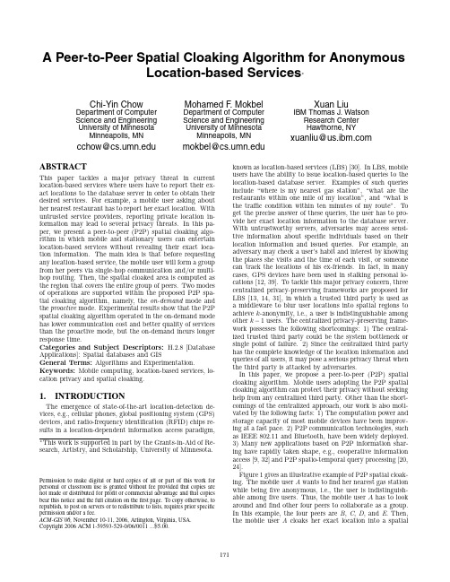
A Peer-to-Peer Spatial Cloaking Algorithm for AnonymousLocation-based Services∗Chi-Yin Chow Department of Computer Science and Engineering University of Minnesota Minneapolis,MN cchow@ Mohamed F.MokbelDepartment of ComputerScience and EngineeringUniversity of MinnesotaMinneapolis,MNmokbel@Xuan LiuIBM Thomas J.WatsonResearch CenterHawthorne,NYxuanliu@ABSTRACTThis paper tackles a major privacy threat in current location-based services where users have to report their ex-act locations to the database server in order to obtain their desired services.For example,a mobile user asking about her nearest restaurant has to report her exact location.With untrusted service providers,reporting private location in-formation may lead to several privacy threats.In this pa-per,we present a peer-to-peer(P2P)spatial cloaking algo-rithm in which mobile and stationary users can entertain location-based services without revealing their exact loca-tion information.The main idea is that before requesting any location-based service,the mobile user will form a group from her peers via single-hop communication and/or multi-hop routing.Then,the spatial cloaked area is computed as the region that covers the entire group of peers.Two modes of operations are supported within the proposed P2P spa-tial cloaking algorithm,namely,the on-demand mode and the proactive mode.Experimental results show that the P2P spatial cloaking algorithm operated in the on-demand mode has lower communication cost and better quality of services than the proactive mode,but the on-demand incurs longer response time.Categories and Subject Descriptors:H.2.8[Database Applications]:Spatial databases and GISGeneral Terms:Algorithms and Experimentation. Keywords:Mobile computing,location-based services,lo-cation privacy and spatial cloaking.1.INTRODUCTIONThe emergence of state-of-the-art location-detection de-vices,e.g.,cellular phones,global positioning system(GPS) devices,and radio-frequency identiﬁcation(RFID)chips re-sults in a location-dependent information access paradigm,∗This work is supported in part by the Grants-in-Aid of Re-search,Artistry,and Scholarship,University of Minnesota. Permission to make digital or hard copies of all or part of this work for personal or classroom use is granted without fee provided that copies are not made or distributed for proﬁt or commercial advantage and that copies bear this notice and the full citation on theﬁrst page.To copy otherwise,to republish,to post on servers or to redistribute to lists,requires prior speciﬁc permission and/or a fee.ACM-GIS’06,November10-11,2006,Arlington,Virginia,USA. Copyright2006ACM1-59593-529-0/06/0011...$5.00.known as location-based services(LBS)[30].In LBS,mobile users have the ability to issue location-based queries to the location-based database server.Examples of such queries include“where is my nearest gas station”,“what are the restaurants within one mile of my location”,and“what is the traﬃc condition within ten minutes of my route”.To get the precise answer of these queries,the user has to pro-vide her exact location information to the database server. With untrustworthy servers,adversaries may access sensi-tive information about speciﬁc individuals based on their location information and issued queries.For example,an adversary may check a user’s habit and interest by knowing the places she visits and the time of each visit,or someone can track the locations of his ex-friends.In fact,in many cases,GPS devices have been used in stalking personal lo-cations[12,39].To tackle this major privacy concern,three centralized privacy-preserving frameworks are proposed for LBS[13,14,31],in which a trusted third party is used as a middleware to blur user locations into spatial regions to achieve k-anonymity,i.e.,a user is indistinguishable among other k−1users.The centralized privacy-preserving frame-work possesses the following shortcomings:1)The central-ized trusted third party could be the system bottleneck or single point of failure.2)Since the centralized third party has the complete knowledge of the location information and queries of all users,it may pose a serious privacy threat when the third party is attacked by adversaries.In this paper,we propose a peer-to-peer(P2P)spatial cloaking algorithm.Mobile users adopting the P2P spatial cloaking algorithm can protect their privacy without seeking help from any centralized third party.Other than the short-comings of the centralized approach,our work is also moti-vated by the following facts:1)The computation power and storage capacity of most mobile devices have been improv-ing at a fast pace.2)P2P communication technologies,such as IEEE802.11and Bluetooth,have been widely deployed.3)Many new applications based on P2P information shar-ing have rapidly taken shape,e.g.,cooperative information access[9,32]and P2P spatio-temporal query processing[20, 24].Figure1gives an illustrative example of P2P spatial cloak-ing.The mobile user A wants toﬁnd her nearest gas station while beingﬁve anonymous,i.e.,the user is indistinguish-able amongﬁve users.Thus,the mobile user A has to look around andﬁnd other four peers to collaborate as a group. In this example,the four peers are B,C,D,and E.Then, the mobile user A cloaks her exact location into a spatialA B CDEBase Stationregion that covers the entire group of mobile users A ,B ,C ,D ,and E .The mobile user A randomly selects one of the mobile users within the group as an agent .In the ex-ample given in Figure 1,the mobile user D is selected as an agent.Then,the mobile user A sends her query (i.e.,what is the nearest gas station)along with her cloaked spa-tial region to the agent.The agent forwards the query to the location-based database server through a base station.Since the location-based database server processes the query based on the cloaked spatial region,it can only give a list of candidate answers that includes the actual answers and some false positives.After the agent receives the candidate answers,it forwards the candidate answers to the mobile user A .Finally,the mobile user A gets the actual answer by ﬁltering out all the false positives.The proposed P2P spatial cloaking algorithm can operate in two modes:on-demand and proactive .In the on-demand mode,mobile clients execute the cloaking algorithm when they need to access information from the location-based database server.On the other side,in the proactive mode,mobile clients periodically look around to ﬁnd the desired number of peers.Thus,they can cloak their exact locations into spatial regions whenever they want to retrieve informa-tion from the location-based database server.In general,the contributions of this paper can be summarized as follows:1.We introduce a distributed system architecture for pro-viding anonymous location-based services (LBS)for mobile users.2.We propose the ﬁrst P2P spatial cloaking algorithm for mobile users to entertain high quality location-based services without compromising their privacy.3.We provide experimental evidence that our proposed algorithm is eﬃcient in terms of the response time,is scalable to large numbers of mobile clients,and is eﬀective as it provides high-quality services for mobile clients without the need of exact location information.The rest of this paper is organized as follows.Section 2highlights the related work.The system model of the P2P spatial cloaking algorithm is presented in Section 3.The P2P spatial cloaking algorithm is described in Section 4.Section 5discusses the integration of the P2P spatial cloak-ing algorithm with privacy-aware location-based database servers.Section 6depicts the experimental evaluation of the P2P spatial cloaking algorithm.Finally,Section 7con-cludes this paper.2.RELATED WORKThe k -anonymity model [37,38]has been widely used in maintaining privacy in databases [5,26,27,28].The main idea is to have each tuple in the table as k -anonymous,i.e.,indistinguishable among other k −1tuples.Although we aim for the similar k -anonymity model for the P2P spatial cloaking algorithm,none of these techniques can be applied to protect user privacy for LBS,mainly for the following four reasons:1)These techniques preserve the privacy of the stored data.In our model,we aim not to store the data at all.Instead,we store perturbed versions of the data.Thus,data privacy is managed before storing the data.2)These approaches protect the data not the queries.In anonymous LBS,we aim to protect the user who issues the query to the location-based database server.For example,a mobile user who wants to ask about her nearest gas station needs to pro-tect her location while the location information of the gas station is not protected.3)These approaches guarantee the k -anonymity for a snapshot of the database.In LBS,the user location is continuously changing.Such dynamic be-havior calls for continuous maintenance of the k -anonymity model.(4)These approaches assume a uniﬁed k -anonymity requirement for all the stored records.In our P2P spatial cloaking algorithm,k -anonymity is a user-speciﬁed privacy requirement which may have a diﬀerent value for each user.Motivated by the privacy threats of location-detection de-vices [1,4,6,40],several research eﬀorts are dedicated to protect the locations of mobile users (e.g.,false dummies [23],landmark objects [18],and location perturbation [10,13,14]).The most closed approaches to ours are two centralized spatial cloaking algorithms,namely,the spatio-temporal cloaking [14]and the CliqueCloak algorithm [13],and one decentralized privacy-preserving algorithm [23].The spatio-temporal cloaking algorithm [14]assumes that all users have the same k -anonymity requirements.Furthermore,it lacks the scalability because it deals with each single request of each user individually.The CliqueCloak algorithm [13]as-sumes a diﬀerent k -anonymity requirement for each user.However,since it has large computation overhead,it is lim-ited to a small k -anonymity requirement,i.e.,k is from 5to 10.A decentralized privacy-preserving algorithm is proposed for LBS [23].The main idea is that the mobile client sends a set of false locations,called dummies ,along with its true location to the location-based database server.However,the disadvantages of using dummies are threefold.First,the user has to generate realistic dummies to pre-vent the adversary from guessing its true location.Second,the location-based database server wastes a lot of resources to process the dummies.Finally,the adversary may esti-mate the user location by using cellular positioning tech-niques [34],e.g.,the time-of-arrival (TOA),the time diﬀer-ence of arrival (TDOA)and the direction of arrival (DOA).Although several existing distributed group formation al-gorithms can be used to ﬁnd peers in a mobile environment,they are not designed for privacy preserving in LBS.Some algorithms are limited to only ﬁnding the neighboring peers,e.g.,lowest-ID [11],largest-connectivity (degree)[33]and mobility-based clustering algorithms [2,25].When a mo-bile user with a strict privacy requirement,i.e.,the value of k −1is larger than the number of neighboring peers,it has to enlist other peers for help via multi-hop routing.Other algorithms do not have this limitation,but they are designed for grouping stable mobile clients together to facil-Location-based Database ServerDatabase ServerDatabase ServerFigure 2:The system architectureitate eﬃcient data replica allocation,e.g.,dynamic connec-tivity based group algorithm [16]and mobility-based clus-tering algorithm,called DRAM [19].Our work is diﬀerent from these approaches in that we propose a P2P spatial cloaking algorithm that is dedicated for mobile users to dis-cover other k −1peers via single-hop communication and/or via multi-hop routing,in order to preserve user privacy in LBS.3.SYSTEM MODELFigure 2depicts the system architecture for the pro-posed P2P spatial cloaking algorithm which contains two main components:mobile clients and location-based data-base server .Each mobile client has its own privacy proﬁle that speciﬁes its desired level of privacy.A privacy proﬁle includes two parameters,k and A min ,k indicates that the user wants to be k -anonymous,i.e.,indistinguishable among k users,while A min speciﬁes the minimum resolution of the cloaked spatial region.The larger the value of k and A min ,the more strict privacy requirements a user needs.Mobile users have the ability to change their privacy proﬁle at any time.Our employed privacy proﬁle matches the privacy re-quirements of mobiles users as depicted by several social science studies (e.g.,see [4,15,17,22,29]).In this architecture,each mobile user is equipped with two wireless network interface cards;one of them is dedicated to communicate with the location-based database server through the base station,while the other one is devoted to the communication with other peers.A similar multi-interface technique has been used to implement IP multi-homing for stream control transmission protocol (SCTP),in which a machine is installed with multiple network in-terface cards,and each assigned a diﬀerent IP address [36].Similarly,in mobile P2P cooperation environment,mobile users have a network connection to access information from the server,e.g.,through a wireless modem or a base station,and the mobile users also have the ability to communicate with other peers via a wireless LAN,e.g.,IEEE 802.11or Bluetooth [9,24,32].Furthermore,each mobile client is equipped with a positioning device, e.g.,GPS or sensor-based local positioning systems,to determine its current lo-cation information.4.P2P SPATIAL CLOAKINGIn this section,we present the data structure and the P2P spatial cloaking algorithm.Then,we describe two operation modes of the algorithm:on-demand and proactive .4.1Data StructureThe entire system area is divided into grid.The mobile client communicates with each other to discover other k −1peers,in order to achieve the k -anonymity requirement.TheAlgorithm 1P2P Spatial Cloaking:Request Originator m 1:Function P2PCloaking-Originator (h ,k )2://Phase 1:Peer searching phase 3:The hop distance h is set to h4:The set of discovered peers T is set to {∅},and the number ofdiscovered peers k =|T |=05:while k <k −1do6:Broadcast a FORM GROUP request with the parameter h (Al-gorithm 2gives the response of each peer p that receives this request)7:T is the set of peers that respond back to m by executingAlgorithm 28:k =|T |;9:if k <k −1then 10:if T =T then 11:Suspend the request 12:end if 13:h ←h +1;14:T ←T ;15:end if 16:end while17://Phase 2:Location adjustment phase 18:for all T i ∈T do19:|mT i .p |←the greatest possible distance between m and T i .pby considering the timestamp of T i .p ’s reply and maximum speed20:end for21://Phase 3:Spatial cloaking phase22:Form a group with k −1peers having the smallest |mp |23:h ←the largest hop distance h p of the selected k −1peers 24:Determine a grid area A that covers the entire group 25:if A <A min then26:Extend the area of A till it covers A min 27:end if28:Randomly select a mobile client of the group as an agent 29:Forward the query and A to the agentmobile client can thus blur its exact location into a cloaked spatial region that is the minimum grid area covering the k −1peers and itself,and satisﬁes A min as well.The grid area is represented by the ID of the left-bottom and right-top cells,i.e.,(l,b )and (r,t ).In addition,each mobile client maintains a parameter h that is the required hop distance of the last peer searching.The initial value of h is equal to one.4.2AlgorithmFigure 3gives a running example for the P2P spatial cloaking algorithm.There are 15mobile clients,m 1to m 15,represented as solid circles.m 8is the request originator,other black circles represent the mobile clients received the request from m 8.The dotted circles represent the commu-nication range of the mobile client,and the arrow represents the movement direction.Algorithms 1and 2give the pseudo code for the request originator (denoted as m )and the re-quest receivers (denoted as p ),respectively.In general,the algorithm consists of the following three phases:Phase 1:Peer searching phase .The request origina-tor m wants to retrieve information from the location-based database server.m ﬁrst sets h to h ,a set of discovered peers T to {∅}and the number of discovered peers k to zero,i.e.,|T |.(Lines 3to 4in Algorithm 1).Then,m broadcasts a FORM GROUP request along with a message sequence ID and the hop distance h to its neighboring peers (Line 6in Algorithm 1).m listens to the network and waits for the reply from its neighboring peers.Algorithm 2describes how a peer p responds to the FORM GROUP request along with a hop distance h and aFigure3:P2P spatial cloaking algorithm.Algorithm2P2P Spatial Cloaking:Request Receiver p1:Function P2PCloaking-Receiver(h)2://Let r be the request forwarder3:if the request is duplicate then4:Reply r with an ACK message5:return;6:end if7:h p←1;8:if h=1then9:Send the tuple T=<p,(x p,y p),v maxp ,t p,h p>to r10:else11:h←h−1;12:Broadcast a FORM GROUP request with the parameter h 13:T p is the set of peers that respond back to p14:for all T i∈T p do15:T i.h p←T i.h p+1;16:end for17:T p←T p∪{<p,(x p,y p),v maxp ,t p,h p>};18:Send T p back to r19:end ifmessage sequence ID from another peer(denoted as r)that is either the request originator or the forwarder of the re-quest.First,p checks if it is a duplicate request based on the message sequence ID.If it is a duplicate request,it sim-ply replies r with an ACK message without processing the request.Otherwise,p processes the request based on the value of h:Case1:h= 1.p turns in a tuple that contains its ID,current location,maximum movement speed,a timestamp and a hop distance(it is set to one),i.e.,< p,(x p,y p),v max p,t p,h p>,to r(Line9in Algorithm2). Case2:h> 1.p decrements h and broadcasts the FORM GROUP request with the updated h and the origi-nal message sequence ID to its neighboring peers.p keeps listening to the network,until it collects the replies from all its neighboring peers.After that,p increments the h p of each collected tuple,and then it appends its own tuple to the collected tuples T p.Finally,it sends T p back to r (Lines11to18in Algorithm2).After m collects the tuples T from its neighboring peers, if m cannotﬁnd other k−1peers with a hop distance of h,it increments h and re-broadcasts the FORM GROUP request along with a new message sequence ID and h.m repeatedly increments h till itﬁnds other k−1peers(Lines6to14in Algorithm1).However,if mﬁnds the same set of peers in two consecutive broadcasts,i.e.,with hop distances h and h+1,there are not enough connected peers for m.Thus, m has to relax its privacy proﬁle,i.e.,use a smaller value of k,or to be suspended for a period of time(Line11in Algorithm1).Figures3(a)and3(b)depict single-hop and multi-hop peer searching in our running example,respectively.In Fig-ure3(a),the request originator,m8,(e.g.,k=5)canﬁnd k−1peers via single-hop communication,so m8sets h=1. Since h=1,its neighboring peers,m5,m6,m7,m9,m10, and m11,will not further broadcast the FORM GROUP re-quest.On the other hand,in Figure3(b),m8does not connect to k−1peers directly,so it has to set h>1.Thus, its neighboring peers,m7,m10,and m11,will broadcast the FORM GROUP request along with a decremented hop dis-tance,i.e.,h=h−1,and the original message sequence ID to their neighboring peers.Phase2:Location adjustment phase.Since the peer keeps moving,we have to capture the movement between the time when the peer sends its tuple and the current time. For each received tuple from a peer p,the request originator, m,determines the greatest possible distance between them by an equation,|mp |=|mp|+(t c−t p)×v max p,where |mp|is the Euclidean distance between m and p at time t p,i.e.,|mp|=(x m−x p)2+(y m−y p)2,t c is the currenttime,t p is the timestamp of the tuple and v maxpis the maximum speed of p(Lines18to20in Algorithm1).In this paper,a conservative approach is used to determine the distance,because we assume that the peer will move with the maximum speed in any direction.If p gives its movement direction,m has the ability to determine a more precise distance between them.Figure3(c)illustrates that,for each discovered peer,the circle represents the largest region where the peer can lo-cate at time t c.The greatest possible distance between the request originator m8and its discovered peer,m5,m6,m7, m9,m10,or m11is represented by a dotted line.For exam-ple,the distance of the line m8m 11is the greatest possible distance between m8and m11at time t c,i.e.,|m8m 11|. Phase3:Spatial cloaking phase.In this phase,the request originator,m,forms a virtual group with the k−1 nearest peers,based on the greatest possible distance be-tween them(Line22in Algorithm1).To adapt to the dynamic network topology and k-anonymity requirement, m sets h to the largest value of h p of the selected k−1 peers(Line15in Algorithm1).Then,m determines the minimum grid area A covering the entire group(Line24in Algorithm1).If the area of A is less than A min,m extends A,until it satisﬁes A min(Lines25to27in Algorithm1). Figure3(c)gives the k−1nearest peers,m6,m7,m10,and m11to the request originator,m8.For example,the privacy proﬁle of m8is(k=5,A min=20cells),and the required cloaked spatial region of m8is represented by a bold rectan-gle,as depicted in Figure3(d).To issue the query to the location-based database server anonymously,m randomly selects a mobile client in the group as an agent(Line28in Algorithm1).Then,m sendsthe query along with the cloaked spatial region,i.e.,A,to the agent(Line29in Algorithm1).The agent forwards thequery to the location-based database server.After the serverprocesses the query with respect to the cloaked spatial re-gion,it sends a list of candidate answers back to the agent.The agent forwards the candidate answer to m,and then mﬁlters out the false positives from the candidate answers. 4.3Modes of OperationsThe P2P spatial cloaking algorithm can operate in twomodes,on-demand and proactive.The on-demand mode:The mobile client only executesthe algorithm when it needs to retrieve information from the location-based database server.The algorithm operatedin the on-demand mode generally incurs less communica-tion overhead than the proactive mode,because the mobileclient only executes the algorithm when necessary.However,it suﬀers from a longer response time than the algorithm op-erated in the proactive mode.The proactive mode:The mobile client adopting theproactive mode periodically executes the algorithm in back-ground.The mobile client can cloak its location into a spa-tial region immediately,once it wants to communicate withthe location-based database server.The proactive mode pro-vides a better response time than the on-demand mode,but it generally incurs higher communication overhead and giveslower quality of service than the on-demand mode.5.ANONYMOUS LOCATION-BASEDSERVICESHaving the spatial cloaked region as an output form Algo-rithm1,the mobile user m sends her request to the location-based server through an agent p that is randomly selected.Existing location-based database servers can support onlyexact point locations rather than cloaked regions.In or-der to be able to work with a spatial region,location-basedservers need to be equipped with a privacy-aware queryprocessor(e.g.,see[29,31]).The main idea of the privacy-aware query processor is to return a list of candidate answerrather than the exact query answer.Then,the mobile user m willﬁlter the candidate list to eliminate its false positives andﬁnd its exact answer.The tighter the spatial cloaked re-gion,the lower is the size of the candidate answer,and hencethe better is the performance of the privacy-aware query processor.However,tight cloaked regions may represent re-laxed privacy constrained.Thus,a trade-oﬀbetween the user privacy and the quality of service can be achieved[31]. Figure4(a)depicts such scenario by showing the data stored at the server side.There are32target objects,i.e., gas stations,T1to T32represented as black circles,the shaded area represents the spatial cloaked area of the mo-bile client who issued the query.For clariﬁcation,the actual mobile client location is plotted in Figure4(a)as a black square inside the cloaked area.However,such information is neither stored at the server side nor revealed to the server. The privacy-aware query processor determines a range that includes all target objects that are possibly contributing to the answer given that the actual location of the mobile client could be anywhere within the shaded area.The range is rep-resented as a bold rectangle,as depicted in Figure4(b).The server sends a list of candidate answers,i.e.,T8,T12,T13, T16,T17,T21,and T22,back to the agent.The agent next for-(a)Server Side(b)Client SideFigure4:Anonymous location-based services wards the candidate answers to the requesting mobile client either through single-hop communication or through multi-hop routing.Finally,the mobile client can get the actualanswer,i.e.,T13,byﬁltering out the false positives from thecandidate answers.The algorithmic details of the privacy-aware query proces-sor is beyond the scope of this paper.Interested readers are referred to[31]for more details.6.EXPERIMENTAL RESULTSIn this section,we evaluate and compare the scalabilityand eﬃciency of the P2P spatial cloaking algorithm in boththe on-demand and proactive modes with respect to the av-erage response time per query,the average number of mes-sages per query,and the size of the returned candidate an-swers from the location-based database server.The queryresponse time in the on-demand mode is deﬁned as the timeelapsed between a mobile client starting to search k−1peersand receiving the candidate answers from the agent.On theother hand,the query response time in the proactive mode is deﬁned as the time elapsed between a mobile client startingto forward its query along with the cloaked spatial regionto the agent and receiving the candidate answers from theagent.The simulation model is implemented in C++usingCSIM[35].In all the experiments in this section,we consider an in-dividual random walk model that is based on“random way-point”model[7,8].At the beginning,the mobile clientsare randomly distributed in a spatial space of1,000×1,000square meters,in which a uniform grid structure of100×100cells is constructed.Each mobile client randomly chooses itsown destination in the space with a randomly determined speed s from a uniform distribution U(v min,v max).When the mobile client reaches the destination,it comes to a stand-still for one second to determine its next destination.Afterthat,the mobile client moves towards its new destinationwith another speed.All the mobile clients repeat this move-ment behavior during the simulation.The time interval be-tween two consecutive queries generated by a mobile client follows an exponential distribution with a mean of ten sec-onds.All the experiments consider one half-duplex wirelesschannel for a mobile client to communicate with its peers with a total bandwidth of2Mbps and a transmission range of250meters.When a mobile client wants to communicate with other peers or the location-based database server,it has to wait if the requested channel is busy.In the simulated mobile environment,there is a centralized location-based database server,and one wireless communication channel between the location-based database server and the mobile。

dfs序列和bfs序列

dfs序列和bfs序列dfs序列和bfs序列是图遍历算法中的两种常见序列。

它们分别代表了深度优先搜索（Depth-First Search）和广度优先搜索（Breadth-First Search）在图中遍历节点的顺序。

1. DFS序列深度优先搜索是一种以深度为优先级的遍历算法。

它从图的起始节点开始，一直沿着一个分支遍历到底，然后回溯到前一个节点，再遍历下一个分支。

这样直到遍历完所有的节点。

DFS序列的生成是通过递归或栈的方式完成的。

在递归实现中，每次深入某个节点时，都对其邻接节点进行深度优先遍历，直到遍历完所有节点为止。

生成的DFS序列可以用一个数组来表示，序列中每个节点的顺序即为其被遍历到的顺序。

2. BFS序列广度优先搜索是一种以广度为优先级的遍历算法。

它从图的起始节点开始，首先遍历其所有的邻接节点，然后再逐层遍历下一个邻接节点的邻接节点。

这样依次遍历完所有的节点。

BFS序列的生成是通过队列的方式完成的。

首先将起始节点入队，然后从队列中依次取出节点，并将其所有未被访问的邻接节点入队，直到队列为空为止。

生成的BFS序列可以用一个数组来表示，序列中每个节点的顺序即为其被遍历到的顺序。

3. DFS序列和BFS序列的应用DFS序列和BFS序列在图遍历算法中具有不同的应用场景。

DFS适用于解决一些涉及路径搜索、连通性、拓扑排序等问题。

由于DFS的特点是往深层次搜索，因此在找到目标节点后可以停止搜索，适合在有限深度的图中应用。

而BFS适用于解决一些涉及最短路径、最小生成树、社交网络分析等问题。

由于BFS的特点是逐层遍历，因此可以保证找到的路径是最短路径，并且可以用于计算节点之间的距离。

总结：DFS序列和BFS序列是图遍历算法中常见的两种序列。

DFS以深度为优先级，递归或栈实现，适合解决路径搜索等问题。

BFS以广度为优先级，队列实现，适合解决最短路径等问题。

对于不同的应用场景，可以选择使用适合的算法序列来进行图遍历。

罗伯特交叉梯度算子例题

罗伯特交叉梯度算子例题罗伯特交叉梯度算子是一种经典的边缘检测算子，它可以帮助我们在图像中检测出边缘的位置。

这个算子是由罗伯特·C·加德（Robert C. Roberts）于1973年提出的，它利用了图像中相邻像素之间的差异来识别边缘。

为了更好地理解罗伯特交叉梯度算子的原理，我们可以通过一个简单的例题来说明。

假设我们有一个3x3的图像矩阵如下：1 2 3。

4 5 6。

7 8 9。

我们可以使用罗伯特交叉梯度算子来计算每个像素点的边缘强度。

具体地，我们可以使用以下两个3x3的卷积核（也称为罗伯特算子）来进行卷积操作：Gx = [[1, 0, 0], [0, -1, 0], [0, 0, 0]]Gy = [[0, 1, 0], [-1, 0, 0], [0, 0, 0]]其中，Gx是用来检测水平边缘的卷积核，Gy是用来检测垂直边缘的卷积核。

我们分别将这两个卷积核与原始图像进行卷积操作，得到水平方向和垂直方向的边缘强度。

对于上述的3x3图像矩阵，我们可以计算出每个像素点的水平和垂直边缘强度。

例如，对于像素点(2,2)处的像素值5，我们可以使用以下公式来计算水平和垂直边缘强度：水平边缘强度，Gx = (6-4) = 2。

垂直边缘强度，Gy = (2-8) = -6。

通过计算所有像素点的水平和垂直边缘强度，我们可以得到整个图像的边缘信息。

一般来说，我们可以将水平和垂直边缘强度进行合并，得到最终的边缘强度。

在实际应用中，我们可以设定一个阈值来筛选出边缘强度大于阈值的像素点，从而得到图像的边缘信息。

总的来说，罗伯特交叉梯度算子通过计算图像中相邻像素之间的差异来检测边缘，它是一种简单而有效的边缘检测算子。

在实际应用中，它常常被用于计算机视觉和图像处理领域，用来帮助识别图像中的边缘信息。

改进的 km 算法流程 -回复

改进的km 算法流程-回复改进的KM算法流程引言KM算法，即Kuhn-Munkres算法，也被称为匈牙利算法，是一种用于解决二分图最大权匹配问题的经典算法。

它在应用中被广泛使用，例如在任务分配、资源分配、航线规划等领域。

然而，KM算法在处理大规模问题时存在效率低下的问题。

为了提高算法的性能，学者们不断进行改进和优化。

本文将介绍改进后的KM算法的流程，并逐步解释每个步骤的具体操作。

一、问题描述在介绍改进的KM算法之前，首先需要明确问题的描述。

给定一个二分图，其中左侧顶点集合为X，右侧顶点集合为Y，边权重矩阵为C。

目标是找到一个匹配M，使得M中所有边的权重之和最大。

二、改进算法的基本思路改进的KM算法主要通过两个步骤来提高效率：启发式初始化和优化的增广路径寻找。

1. 启发式初始化：将初始标号设置为最小权重值2. 优化的增广路径寻找：通过DFS（深度优先搜索）和BFS（广度优先搜索）寻找增广路径下面将详细介绍这两个步骤。

三、启发式初始化启发式初始化的目的是在算法初始阶段就为每个顶点设置一个初始标号，以便减少后续迭代中的计算量。

具体步骤如下：1. 初始化顶点集合X和Y的标号为0。

2. 对于每个左侧顶点x∈X，找到该顶点对应的最大权重，将该权重作为左侧顶点x的初始标号。

3. 更新右侧顶点y∈Y的标号为与它相连的左侧顶点的初始标号中的最大值。

四、优化的增广路径寻找优化的增广路径寻找是通过DFS和BFS结合的方式来寻找增广路径，其中DFS用于尽可能延伸已有的匹配集，而BFS用于寻找未被匹配的顶点。

1. 初始化路径集合P为空。

2. 对于每个未匹配的左侧顶点x∈X，将x添加到路径集合P中。

3. 对于路径集合P中的每个顶点u，如果u是未匹配的左侧顶点，则将u的相邻未匹配右侧顶点v添加到路径集合P中，并将v的前驱节点设置为u。

4. 如果路径集合P中存在一条从未匹配的左侧顶点x开始，以交替的形式经过已匹配的边和未匹配的边，并最终达到未匹配的右侧顶点y的路径，那么就找到了一条增广路径。

算法基础：BFS和DFS的直观解释

算法基础：BFS和DFS的直观解释算法基础：BFS和DFS的直观解释https:///blog/2018/01/alogrithm_10.html算法基础：BFS和DFS的直观解释⼀、前⾔我们⾸次接触和 DFS 时，应该是在数据结构课上讲的 “图的遍历”。

还有就是刷题的时候，遍历⼆叉树我们会经常⽤到和DFS。

它们的实现都很简单，这⾥我就不哆嗦去贴代码了。

想看代码的可以看《》这个题⽬就可以利⽤BFS和DFS进⾏求解。

那么，这两者“遍历” 的序列到底有何差别？本篇⽂章就单纯来讲讲它们的区别和各⾃的应⽤，不会涉及任何代码。

我们以“图的遍历”为例，进⾏说明。

⼆、区别⼴度优先搜索算法（Breadth-First-Search，缩写为 BFS），是⼀种利⽤队列实现的搜索算法。

简单来说，其搜索过程和 “湖⾯丢进⼀块⽯头激起层层涟漪” 类似。

深度优先搜索算法（Depth-First-Search，缩写为 DFS），是⼀种利⽤递归实现的搜索算法。

简单来说，其搜索过程和 “不撞南墙不回头” 类似。

BFS 的重点在于队列，⽽ DFS 的重点在于递归。

这是它们的本质区别。

举个典型例⼦，如下图，灰⾊代表墙壁，绿⾊代表起点，红⾊代表终点，规定每次只能⾛⼀步，且只能往下或右⾛。

求⼀条绿⾊到红⾊的最短路径。

对于上⾯的问题，BFS 和 DFS 都可以求出结果，它们的区别就是在复杂度上存在差异。

我可以先告诉你，该题 BFS 是较佳算法。

BFS⽰意图：如上图所⽰，从起点出发，对于每次出队列的点，都要遍历其四周的点。

所以说 BFS 的搜索过程和 “湖⾯丢进⼀块⽯头激起层层涟漪” 很相似，此即 “⼴度优先搜索算法” 中“⼴度”的由来。

DFS⽰意图：如上图所⽰，从起点出发，先把⼀个⽅向的点都遍历完才会改变⽅向...... 所以说，DFS 的搜索过程和 “不撞南墙不回头” 很相似，此即 “深度优先搜索算法” 中“深度”的由来。

三、总结现在，你不妨对照着图，再去看看你打印出的遍历序列，是不是⼀⽬了然呢？最后再说下它们的应⽤⽅向。

BFS和DFS详解以及java实现（转载）

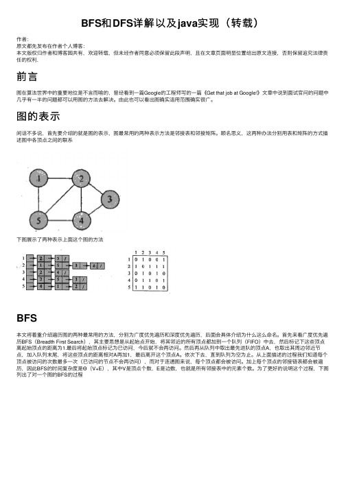
BFS和DFS详解以及java实现（转载）作者：原⽂都先发布在作者个⼈博客：本⽂版权归作者和博客园共有，欢迎转载，但未经作者同意必须保留此段声明，且在⽂章页⾯明显位置给出原⽂连接，否则保留追究法律责任的权利.前⾔图在算法世界中的重要地位是不⾔⽽喻的，曾经看到⼀篇Google的⼯程师写的⼀篇《Get that job at Google!》⽂章中说到⾯试官问的问题中⼏乎有⼀半的问题都可以⽤图的⽅法去解决。

由此也可以看出图确实适⽤范围确实很⼴。

图的表⽰闲话不多说，⾸先要介绍的就是图的表⽰，图最常⽤的两种表⽰⽅法是邻接表和邻接矩阵。

顾名思义，这两种办法分别⽤表和矩阵的⽅式描述图中各顶点之间的联系下图展⽰了两种表⽰上⾯这个图的⽅法BFS本⽂将着重介绍遍历图的两种最常⽤的⽅法，分别为⼴度优先遍历和深度优先遍历，后⾯会具体介绍为什么这么命名。

⾸先来看⼴度优先遍历BFS（Breadth First Search），其主要思想是从起始点开始，将其邻近的所有顶点都加到⼀个队列（FIFO）中去，然后标记下这些顶点离起始顶点的距离为1.最后将起始顶点标记为已访问，今后就不会再访问。

然后再从队列中取出最先进队的顶点A，也取出其周边邻近节点，加⼊队列末尾，将这些顶点的距离相对A再加1，最后离开这个顶点A。

依次下去，直到队列为空为⽌。

从上⾯描述的过程我们知道每个顶点被访问的次数最多⼀次（已访问的节点不会再访问），⽽对于连通图来说，每个顶点都会被访问。

加上每个顶点的邻接链表都会被遍历，因此BFS的时间复杂度是Θ（V+E），其中V是顶点个数，E是边数，也就是所有邻接表中的元素个数。

为了更好的说明这个过程，下图列出了对⼀个图的BFS的过程private static void bfs(HashMap<Character, LinkedList<Character>> graph,HashMap<Character, Integer> dist,char start){Queue<Character> q=new LinkedList<>();q.add(start);//将s作为起始顶点加⼊队列dist.put(start, 0);int i=0;while(!q.isEmpty()){char top=q.poll();//取出队⾸元素i++;System.out.println("The "+i+"th element:"+top+" Distance from s is:"+dist.get(top));int d=dist.get(top)+1;//得出其周边还未被访问的节点的距离for (Character c : graph.get(top)) {if(!dist.containsKey(c))//如果dist中还没有该元素说明还没有被访问{dist.put(c, d);q.add(c);}}}}运⾏结果：从运⾏结果我们也可以看到，w r作为距离为1的顶点先被访问，x t v其后，最后访问y u。

dfs算法实例

dfs算法实例DFS（深度优先搜索）算法是一种常用的图遍历算法，在计算机科学中有着广泛的应用。

本文将以DFS算法为主题，介绍它的原理、应用和实现方式。

一、DFS算法原理深度优先搜索（DFS）是一种用于遍历或搜索树或图的算法。

该算法从起始节点开始，沿着一条路径直到无法继续为止，然后回溯到前一个节点，再沿着另一条路径继续遍历，直到遍历完所有节点。

二、DFS算法应用1. 连通性分析：DFS可以用于判断两个节点是否连通，通过遍历图中的节点，判断是否能从一个节点到达另一个节点。

2. 周游问题：DFS可以用于求解图的周游问题，即找到经过所有节点的路径。

3. 拓扑排序：DFS可以用于对有向无环图进行拓扑排序，即找到一个合理的节点顺序，使得在该顺序下，任意一对节点之间的路径方向均为单向。

4. 迷宫求解：DFS可以用于解决迷宫问题，通过在迷宫中进行深度优先搜索，找到从起点到终点的路径。

三、DFS算法实现方式DFS算法可以通过递归或栈来实现。

以下是使用递归方式实现DFS 算法的伪代码：```function DFS(node):if node is visited:returnmark node as visitedprocess nodefor each neighbor of node:DFS(neighbor)```四、DFS算法实例假设有一个有向图，其中包含节点A、B、C、D、E、F、G。

节点之间的连通关系如下图所示：```A -> BA -> CB -> DB -> EC -> FE -> G```我们以节点A作为起始节点，使用DFS算法遍历该图。

首先访问节点A，然后按照连通关系依次访问节点B、D、E、G、C、F。

最终得到遍历的路径为：A -> B -> D -> E -> G -> C -> F。

五、总结DFS算法是一种常用的图遍历算法，它可以用于解决连通性分析、周游问题、拓扑排序和迷宫求解等。

一种基于灰狼优化算法和Dijkstra的分簇路由协议

一种基于灰狼优化算法和Dijkstra的分簇路由协议
王军;丁丕欣;刘鼎坤
【期刊名称】《火力与指挥控制》
【年(卷),期】2024(49)1
【摘要】针对无线传感器网络分簇路由中簇头能量消耗过快导致生命周期过短的问题,提出一种基于灰狼优化和Dijkstra算法的分簇路由协议。

簇头选举过程中采用灰狼优化算法选取最优簇头,改进适应度函数,综合考虑节点能量、密度、位置、当选簇头频率4个因素;簇间路由采用能量与距离最小权值的Dijkstra算法进行路径选取,完成传感器信息传输。

通过仿真实验显示,该算法与LEACH、PEAGASIS、ABC算法相比,能有效地降低节点死亡速率,均衡网络整体能耗,延长网络寿命。

【总页数】7页(P144-150)
【作者】王军;丁丕欣;刘鼎坤
【作者单位】沈阳化工大学计算机科学与技术学院;辽宁省化工过程工业智能化技术重点实验室
【正文语种】中文
【中图分类】TN929.5;TP212.9
【相关文献】
1.基于嵌套细菌觅食优化算法的WSN分簇路由协议研究
2.WSN中基于改进粒子群优化算法的分簇路由协议
3.一种无线传感器网络分簇路由协议优化算法
4.WSN
中基于改进灰狼优化的分簇路由协议5.基于鲸鱼优化算法和天牛须搜索的WSNs 分簇路由协议
因版权原因，仅展示原文概要，查看原文内容请购买。