【NL-Medians】Non-local euclidean medains
已知的miRNA的ID中英文对照

aae Aedes aegypti 埃及伊蚊aca Anolis carolinensis 安乐蜥aga Anopheles gambiae 冈比亚按蚊aly Arabidopsis lyrata 琴叶拟南芥ame Apis mellifera 意蜂api Acyrthosiphon pisum 豌豆蚜ata Aegilops tauschii 山羊草/节节麦ath Arabidopsis thaliana 拟南芥atr Amborella trichopoda 无油樟bdi Brachypodium distachyon 二穗短柄草blv Bovine leukemia virus 牛白血病病毒bma Brugia malayi 马来丝虫bmo Bombyx mori 家蚕bna Brassica napus 油菜bra Brassica rapa 白菜/芜菁bta Bos T aurus (普通)牛cbn Caenorhabditis brenneri 线虫brennericbr Caenorhabditis briggsae 线虫briggsaecel Caenorhabditis elegans 秀丽隐杆线虫cfa Canis familiaris 家犬chi Capra hircus 山羊cin Ciona intestinalis 玻璃海鞘cqu Culex quinquefasciatus 致倦库蚊cre Chlamydomonas reinhardtii 莱茵衣藻crm Caenorhabditis remanei 线虫remanei csa Ciona savignyi 玻璃海鞘savignyicte Capitella teleta 小头虫teletadan Drosophila ananassae 果蝇ananassaeddi Dictyostelium discoideum 盘基网柄菌der Drosophila erecta 果蝇万寿菊dgr Drosophila grimshawi 果蝇grimshawi dme Drosophila melanogaster 黑腹果蝇dmo Drosophila mojavensis 果蝇mojavensis dpe Drosophila persimilis 果蝇螨dps Drosophila pseudoobscura 果蝇pseudoobscura dpu Daphnia pulex 蚤状溞dre Danio rerio 斑马鱼dse Drosophila sechellia 果蝇sechelliadsi Drosophila simulans 果蝇simulansdvi Drosophila virilis 果蝇virlisdwi Drosophila willistoni 果蝇willistonidya Drosophila yakuba 果蝇yakubaebv Epstein Barr virus EB病毒eca Equus caballus 马efu Eptesicus fuscus 大棕蝠/大棕鲇egr Echinococcus granulosus 细粒棘球绦虫emu Echinococcus multilocularis 多房棘球绦虫esi Ectocarpus siliculosus 水云siliculosusfru Fugu rubripes 红鳍东方鲀gga Gallus gallus 原鸡ggo Gorilla gorilla 大猩猩gma Glycine max 大豆gra Gossypium raimondii 雷蒙德氏棉hbr Hevea brasiliensis 橡胶树hbv Herpes B virus 乙型肝炎病毒hcmv Human cytomegalovirus 人巨细胞病毒hme Heliconius melpomene 红带袖蝶hsa Homo sapiens 智人isc Ixodes scapularis 肩突硬蜱kshv Kaposi sarcoma-associated herpesvirus 卡波济肉瘤相关疱疹病毒lgi Lottia gigantean 帽贝lja Lotus japonicas 百脉根mdm Malus domestica 苹果mdo Monodelphis domestica 短尾负鼠mdv1 Mareks disease virus 马立克氏病病毒mes Manihot esculenta 木薯星虫mghv Mouse gammaherpesvirus 68 小鼠γ疱疹病毒mml Macaca mulatta 猕猴mmu Mus musculus 小家鼠mse Manduca sexta 烟草天蛾mtr Medicago truncatula 蒺藜苜蓿nve Nematostella vectensis海葵nvi Nasonia vitripennis 金小蜂oan Ornithorhynchus anatinus 鸭嘴兽oar Ovis aries 绵羊ocu Oryctolagus cuniculus 家兔oha Ophiophagus Hannah 眼镜王蛇ola Oryzias latipes 青鳉osa Oryza sativa 水稻pma Petromyzon marinus 海七鳃鳗ppc Pristionchus pacificus 蛔虫ppe Prunus persica 桃ppt Physcomitrella patens 小立碗藓ppy Pongo pygmaeus 猩猩prd Panagrellus redivivus 全齿复活线虫/腐生线虫ptc Populus trichocarpa 毛果杨ptr Pan troglodytes 黑猩猩pxy Plutella xylostella 小菜蛾rco Ricinus communis 蓖麻rno Rattus norvegicus 褐家鼠rrv Rhesus monkey rhadinovirus 猕猴Rhadino病毒sbi Sorghum bicolor 高粱sha Sarcophilus harrisii 袋獾sja Schistosoma japonicum 日本血吸虫sko Saccoglossus kowalevskii 橡子蠕虫sly Solanum lycopersicum 番茄sma Schistosoma mansoni 曼氏血吸虫sme Schmidtea mediterranea 淡水涡虫spu Strongylocentrotus purpuratus 紫色球海胆ssc Sus scrofa 野猪str Strongyloides ratti 鼠类圆线虫stu Solanum tuberosum 马铃薯tca Tribolium castaneum 赤拟谷盗tch Tupaia chinensis 树鼩tgu T aeniopygia guttata 斑胸草雀tni Tetraodon nigroviridis 金娃娃vvi Vitis vinifera 葡萄xtr Xenopus tropicalis 热带爪蟾zma Zea mays 玉米。
NLOS identification and mitigation for localization based on UWB experimental data

NLOS Identification and Mitigation for Localization Based on UWB Experimental Data Stefano Maran`o,Student Member,IEEE,Wesley M.Gifford,Student Member,IEEE,Henk Wymeersch,Member,IEEE,Moe Z.Win,Fellow,IEEEAbstract—Sensor networks can benefit greatly from location-awareness,since it allows information gathered by the sensors to be tied to their physical locations.Ultra-wide bandwidth(UWB) transmission is a promising technology for location-aware sensor networks,due to its power efficiency,fine delay resolution,and robust operation in harsh environments.However,the presence of walls and other obstacles presents a significant challenge in terms of localization,as they can result in positively biased distance estimates.We have performed an extensive indoor measurement campaign with FCC-compliant UWB radios to quantify the effect of non-line-of-sight(NLOS)propagation.From these channel pulse responses,we extract features that are representative of the propagation conditions.We then develop classification and regression algorithms based on machine learning techniques, which are capable of:(i)assessing whether a signal was trans-mitted in LOS or NLOS conditions;and(ii)reducing ranging error caused by NLOS conditions.We evaluate the resulting performance through Monte Carlo simulations and compare with existing techniques.In contrast to common probabilistic approaches that require statistical models of the features,the proposed optimization-based approach is more robust against modeling errors.Index Terms—Localization,UWB,NLOS Identification,NLOS Mitigation,Support Vector Machine.I.I NTRODUCTIONL OCATION-AW ARENESS is fast becoming an essential aspect of wireless sensor networks and will enable a myr-iad of applications,in both the commercial and the military sectors[1],[2].Ultra-wide bandwidth(UWB)transmission [3]–[8]provides robust signaling[8],[9],as well as through-wall propagation and high-resolution ranging capabilities[10], [11].Therefore,UWB represents a promising technology for localization applications in harsh environments and accuracy-critical applications[10]–[15].In practical scenarios,however, a number of challenges remain before UWB localization and communication can be deployed.These include signal Manuscript received15May2009;revised15February2010.This research was supported,in part,by the National Science Foundation under grant ECCS-0901034,the Office of Naval Research Presidential Early Career Award for Scientists and Engineers(PECASE)N00014-09-1-0435,the Defense University Research Instrumentation Program under grant N00014-08-1-0826, and the MIT Institute for Soldier Nanotechnologies.S.Maran`o was with Laboratory for Information and Decision Systems (LIDS),Massachusetts Institute of Technology(MIT),and is now with the Swiss Seismological Service,ETH Z¨u rich,Z¨u rich,Switzerland(e-mail: stefano.marano@sed.ethz.ch).H.Wymeersch was with LIDS,MIT,and is now with Chalmers University of Technology,G¨o teborg,Sweden(e-mail:henkw@chalmers.se).Wesley M.Gifford and Moe Z.Win are with LIDS,MIT,Cambridge,MA 02139USA(e-mail:wgifford@,moewin@).Digital Object Identifier10.1109/JSAC.2010.100907.acquisition[16],multi-user interference[17],[18],multipath effects[19],[20],and non-line-of-sight(NLOS)propagation [10],[11].The latter issue is especially critical[10]–[15]for high-resolution localization systems,since NLOS propagation introduces positive biases in distance estimation algorithms, thus seriously affecting the localization performance.Typical harsh environments such as enclosed areas,urban canyons, or under tree canopies inherently have a high occurrence of NLOS situations.It is therefore critical to understand the impact of NLOS conditions on localization systems and to develop techniques that mitigate their effects.There are several ways to deal with ranging bias in NLOS conditions,which we classify as identification and mitigation. NLOS identification attempts to distinguish between LOS and NLOS conditions,and is commonly based on range estimates[21]–[23]or on the channel pulse response(CPR) [24],[25].Recent,detailed overviews of NLOS identification techniques can be found in[22],[26].NLOS mitigation goes beyond identification and attempts to counter the positive bias introduced in NLOS signals.Several techniques[27]–[31]rely on a number of redundant range estimates,both LOS and NLOS,in order to reduce the impact of NLOS range estimates on the estimated agent position.In[32]–[34]the geometry of the environment is explicitly taken into account to cope with NLOS situations.Other approaches,such as[35],attempt to detect the earliest path in the CPR in order to better estimate the TOA in NLOS prehensive overviews of NLOS mitigation techniques can be found in[26],[36]. The main drawbacks of existing NLOS identification and mitigation techniques are:(i)loss of information due to the direct use of ranges instead of the CPRs;(ii)latency incurred during the collection of range estimates to establish a history; and(iii)difficulty in determining the joint probability distribu-tions of the features required by many statistical approaches. In this paper,we consider an optimization-based approach. In particular,we propose the use of non-parametric ma-chine learning techniques to perform NLOS identification and NLOS mitigation.Hence,they do not require a statistical characterization of LOS and NLOS channels,and can perform identification and mitigation under a common framework.The main contributions of this paper are as follows:•characterization of differences in the CPRs under LOS and NLOS conditions based on an extensive indoor mea-surement campaign with FCC-compliant UWB radios;•determination of novel features extracted from the CPR that capture the salient properties in LOS and NLOS conditions;0733-8716/10/$25.00c 2010IEEE•demonstration that a support vector machine (SVM)clas-si fier can be used to distinguish between LOS and NLOS conditions,without the need for statistical modeling of the features under either condition;and•development of SVM regressor-based techniques to mit-igate the ranging bias in NLOS situations,again without the need for statistical modeling of the features under either condition.The remainder of the paper is organized as follows.In Section II,we introduce the system model,problem statement,and describe the effect of NLOS conditions on ranging.In Section III,we describe the equipment and methodologies of the LOS/NLOS measurement campaign and its contribu-tion to this work.The proposed techniques for identi fication and mitigation are described in Section IV,while different strategies for incorporating the proposed techniques within any localization system are discussed in Section V.Numerical performance results are provided in Section VI,and we draw our conclusions in Section VII.II.P ROBLEM S TATEMENT AND S YSTEM M ODEL In this section,we describe the ranging and localization algorithm,and demonstrate the need for NLOS identi fication and mitigation.A.Single-node LocalizationA network consists of two types of nodes:anchors are nodes with known positions,while agents are nodes with unknown positions.For notational convenience,we consider the point of view of a single agent,with unknown position p ,surrounded by N b anchors,with positions,p i ,i =1,...,N b .The distance between the agent and anchor i is d i = p −p i .The agent estimates the distance between itself and the anchors,using a ranging protocol.We denote the estimateddistance between the agent and anchor i by ˆdi ,the ranging error by εi =ˆdi −d i ,the estimate of the ranging error by ˆεi ,the channel condition between the agent and anchor i by λi ∈{LOS ,NLOS },and the estimate of the channelcondition by ˆλi .The mitigated distance estimate of d i is ˆd m i=ˆd i −ˆεi .The residual ranging error after mitigation is de fined as εm i =ˆd m i −d i .Given a set of at least three distance estimates,the agent will then determine its position.While there are numerous positioning algorithms,we focus on the least squares (LS)criterion,due to its simplicity and because it makes no assumptions regarding ranging errors.The agent can infer its position by minimizing the LS cost functionˆp=arg min p(p i ,ˆdi )∈Sˆd i − p −p i 2.(1)Note that we have introduced the concept of the set of useful neighbors S ,consisting of couplesp i ,ˆdi .The optimization problem (1)can be solved numerically using steepest descent.B.Sources of ErrorThe localization algorithm will lead to erroneous results when the ranging errors are large.In practice the estimated distances are not equal to the true distances,because of a number of effects including thermal noise,multipath propa-gation,interference,and ranging algorithm inaccuracies.Ad-ditionally,the direct path between requester and responder may be obstructed,leading to NLOS propagation.In NLOS conditions,the direct path is either attenuated due to through-material propagation,or completely blocked.In the former case,the distance estimates will be positively biased due to the reduced propagation speed (i.e.,less than the expected speed of light,c ).In the latter case the distance estimate is also positively biased,as it corresponds to a re flected path.These bias effects can be accounted for in either the ranging or localization phase.In the remainder of this paper,we focus on techniques that identify and mitigate the effects of NLOS signals during the ranging phase.In NLOS identi fication,the terms in (1)corre-sponding to NLOS distance estimates are omitted.In NLOS mitigation,the distance estimates corresponding to NLOS signals are corrected for improved accuracy.The localization algorithm can then adopt different strategies,depending on the quality and the quantity of available range estimates.III.E XPERIMENTAL A CTIVITIESThis section describes the UWB LOS/NLOS measurement campaign performed at the Massachusetts Institute of Tech-nology by the Wireless Communication and Network Sciences Laboratory during Fall 2007.A.OverviewThe aim of this experimental effort is to build a large database containing a variety of propagation conditions in the indoor of fice environment.The measurements were made using two FCC-compliant UWB radios.These radios repre-sent off-the-shelf transceivers and therefore an appropriate benchmark for developing techniques using currently available technology.The primary focus is to characterize the effects of obstructions.Thus,measurement positions (see Fig.1)were chosen such that half of the collected waveforms were cap-tured in NLOS conditions.The distance between transmitter and receiver varies widely,from roughly 0.6m up to 18m,to capture a variety of operating conditions.Several of fices,hallways,one laboratory,and a large lobby constitute the physical setting of this campaign.While the campaign was conducted in one particular indoor of fice envi-ronment,because of the large number of measurements and the variety of propagation scenarios encountered,we expect that our results are applicable in other of fice environments.The physical arrangement of the campaign is depicted in Fig.1.In each measurement location,the received waveform and the associated range estimate,as well as the actual distance are recorded.The waveforms are then post-processed in order to reduce dependencies on the speci fic algorithm and hardware,e.g.,on the leading edge detection (LED)algorithm embedded in the radios.Fig.1.Measurements were taken in clusters over several different rooms and hallways to capture different propagation conditions.B.Experimental ApparatusThe commercially-available radios used during the data collection process are capable of performing communications and ranging using UWB signals.The radio complies with the emission limit set forth by the FCC[37].Specifically, the10dB bandwidth spans from3.1GHz to6.3GHz.The radio is equipped with a bottom fed planar elliptical antenna. This type of dipole antenna is reported to be well matched and radiation efficient.Most importantly,it is omni-directional and thus suited for ad-hoc networks with arbitrary azimuthal orientation[38].Each radio is mounted on the top of a plastic cart at a height of90cm above the ground.The radios perform a round-trip time-of-arrival(RTOA)ranging protocol1and are capable of capturing waveforms while performing the ranging procedure.Each waveform r(t)captured at the receiving radio is sampled at41.3ps over an observation window of190ns.C.Measurement ArrangementMeasurements were taken at more than one hundred points in the considered area.A map,depicting the topological organization of the clusters within the building,is shown 1RTOA allows ranging between two radios without a common time reference;and thus alleviates the need for networksynchronization.Fig.2.The measurement setup for collecting waveforms between D675CA and H6around the corner of the WCNS Laboratory.in Fig.1,and a typical measurement scenario is shown in Fig.2.Points are placed randomly,but are restricted to areas which are accessible by the carts.The measurement points are grouped into non-overlapping clusters,i.e.,each point only belongs to a single cluster.Typically,a cluster corresponds to a room or a region of a hallway.Within each cluster,measurements between every possible pair of points were captured.When two clusters were within transmission range, every inter-cluster measurement was collected as well.Overall, more than one thousand unique point-to-point measurements were performed.For each pair of points,several received waveforms and distance estimates are recorded,along with the actual distance.During each measurement the radios remain stationary and care is taken to limit movement of other objects in the nearby surroundings.D.DatabaseUsing the measurements collected during the measurement phase,a database was created and used to develop and evaluate the proposed identification and mitigation techniques. It includes1024measurements consisting of512waveforms captured in the LOS condition and512waveforms captured in the NLOS condition.The term LOS is used to denote the existence of a visual path between transmitter and receiver,i.e., a measurement is labeled as LOS when the straight line be-tween the transmitting and receiving antenna is unobstructed. The ranging estimate was obtained by an RTOA algorithm embedded on the radio.The actual position of the radio during each measurement was manually recorded,and the ranging error was calculated with the aid of computer-aided design(CAD)software.The collected waveforms were then processed to align thefirst path in the delay domain using a simple threshold-based method.The alignment process creates a time reference independent of the LED algorithm embedded on the radio.IV.NLOS I DENTIFICATION AND M ITIGATIONThe collected measurement data illustrates that NLOS prop-agation conditions significantly impact ranging performance. For example,Fig.3shows the empirical CDFs of the ranging error over the ensemble of all measurements collected under the two different channel conditions.In LOS conditions a ranging error below one meter occurs in more than95%of the measurements.On the other hand,in NLOS conditions a ranging error below one meter occurs in less than30%of the measurements.Clearly,LOS and NLOS range estimates have very dif-ferent characteristics.In this section,we develop techniques to distinguish between LOS and NLOS situations,and to mitigate the positive biases present in NLOS range estimates. Our techniques are non-parametric,and rely on least-squares support-vector machines(LS-SVM)[39],[40].Wefirst de-scribe the features for distinguishing LOS and NLOS situa-tions,followed by a brief introduction to LS-SVM.We then describe how LS-SVM can be used for NLOS identification and mitigation in localization applications,without needing to determine parametric joint distributions of the features for both the LOS and NLOS conditions.A.Feature Selection for NLOS ClassificationWe have extracted a number of features,which we expect to capture the salient differences between LOS and NLOS signals,from every received waveform r(t).These featuresFig.3.CDF of the ranging error for the LOS and NLOS condition. were selected based on the following observations:(i)in NLOS conditions,signals are considerably more attenuated and have smaller energy and amplitude due to reflections or obstructions;(ii)in LOS conditions,the strongest path of the signal typically corresponds to thefirst path,while in NLOS conditions weak components typically precede the strongest path,resulting in a longer rise time;and(iii)the root-mean-square(RMS)delay spread,which captures the temporal dispersion of the signal’s energy,is larger for NLOS signals. Fig.4depicts two waveforms received in the LOS and NLOS condition supporting our observations.We also include some features that have been presented in the literature.Taking these considerations into account,the features we will consider are as follows:1)Energy of the received signal:E r=+∞−∞|r(t)|2dt(2) 2)Maximum amplitude of the received signal:r max=maxt|r(t)|(3) 3)Rise time:t rise=t H−t L(4) wheret L=min{t:|r(t)|≥ασn}t H=min{t:|r(t)|≥βr max},andσn is the standard deviation of the thermal noise.The values ofα>0and0<β≤1are chosen empirically in order to capture the rise time;in our case, we usedα=6andβ=0.6.4)Mean excess delay:τMED=+∞−∞tψ(t)dt(5) whereψ(t)=|r(t)|2/E r.Fig.4.In some situations there is a clear difference between LOS(upper waveform)and NLOS(lower waveform)signals.5)RMS delay spread:τRMS=+∞−∞(t−τMED)2ψ(t)dt(6)6)Kurtosis:κ=1σ4|r|TT|r(t)|−μ|r|4dt(7)whereμ|r|=1TT|r(t)|dtσ2|r|=1TT|r(t)|−μ|r|2dt.B.Least Squares SVMThe SVM is a supervised learning technique used both for classification and regression problems[41].It represents one of the most widely used classification techniques because of its robustness,its rigorous underpinning,the fact that it requires few user-defined parameters,and its superior performance compared to other techniques such as neural networks.LS-SVM is a low-complexity variation of the standard SVM, which has been applied successfully to classification and regression problems[39],[40].1)Classification:A linear classifier is a function R n→{−1,+1}of the forml(x)=sign[y(x)](8) withy(x)=w Tϕ(x)+b(9) whereϕ(·)is a predetermined function,and w and b are unknown parameters of the classifier.These parameters are de-termined based on the training set{x k,l k}N k=1,where x k∈R n and l k∈{−1,+1}are the inputs and labels,respectively.In the case where the two classes can be separated the SVM determines the separating hyperplane which maximizes the margin between the two classes.2Typically,most practical problems involve classes which are not separable.In this case,the SVM classifier is obtained by solving the following optimization problem:arg minw,b,ξ12w 2+γNk=1ξk(10)s.t.l k y(x k)≥1−ξk,∀k(11)ξk≥0,∀k,(12) where theξk are slack variables that allow the SVM to tolerate misclassifications andγcontrols the trade-off between minimizing training errors and model complexity.It can be shown that the Lagrangian dual is a quadratic program(QP) [40,eqn.2.26].To further simplify the problem,the LS-SVM replaces the inequality(11)by an equality:arg minw,b,e12w 2+γ12Nk=1e2k(13)s.t.l k y(x k)=1−e k,∀k.(14) Now,the Lagrangian dual is a linear program(LP)[40,eqn.3.5],which can be solved efficiently by standard optimization toolboxes.The resulting classifier can be written asl(x)=signNk=1αk l k K(x,x k)+b,(15)whereαk,the Lagrange multipliers,and b are found from the solution of the Lagrangian dual.The function K(x k,x l)=ϕ(x k)Tϕ(x l)is known as the kernel which enables the SVM to perform nonlinear classification.2)Regression:A linear regressor is a function R n→R of the formy(x)=w Tϕ(x)+b(16) whereϕ(·)is a predetermined function,and w and b are unknown parameters of the regressor.These parameters are determined based on the training set{x k,y k}N k=1,where x k∈R n and y k∈R are the inputs and outputs,respectively. The LS-SVM regressor is obtained by solving the following optimization problem:arg minw,b,e12w 2+γ12e 2(17)s.t.y k=y(x k)+e k,∀k,(18) whereγcontrols the trade-off between minimizing training errors and model complexity.Again,the Lagrangian dual is an LP[40,eqn.3.32],whose solution results in the following LS-SVM regressory(x)=Nk=1αk K(x,x k)+b.(19)2The margin is given by1/ w ,and is defined as the smallest distance between the decision boundary w Tϕ(x)+b=0and any of the training examplesϕ(x k).C.LS-SVM for NLOS Identi fication and MitigationWe now apply the non-parametric LS-SVM classi fier to NLOS identi fication,and the LS-SVM regressor to NLOS mitigation.We use 10-fold cross-validation 3to assess the performance of our features and the SVM.Not only are we interested in the performance of LS-SVM for certain features,but we are also interested in which subsets of the available features give the best performance.1)Classi fication:To distinguish between LOS and NLOS signals,we train an LS-SVM classi fier with inputs x k and corresponding labels l k =+1when λk =LOS and l k =−1when λk =NLOS .The input x k is composed of a subset of the features given in Section IV-A.A trade-off between classi fier complexity and performance can be made by using a different size feature subset.2)Regression:To mitigate the effect of NLOS propagation,we train an LS-SVM regressor with inputs x k and corre-sponding outputs y k =εk associated with the NLOS signals.Similar to the classi fication case,x k is composed of a subset of features,selected from those given in Section IV-A and therange estimate ˆdk .Again,the performance achieved by the regressor will depend on the size of the feature subset and the combination of features used.V.L OCALIZATION S TRATEGIESBased on the LS-SVM classi fier and regressor,we can develop the following localization strategies:(i)localization via identi fication ,where only classi fication is employed;(ii)localization via identi fication and mitigation ,where the re-ceived waveform is first classi fied and error mitigation is performed only on the range estimates from those signals identi fied as NLOS;and (iii)a hybrid approach which discards mitigated NLOS range estimates when a suf ficient number of LOS range estimates are present.A.Strategy 1:StandardIn the standard strategy,all the range estimates ˆdi from neighboring anchor nodes are used by the LS algorithm (1)for localization.In other words,S S =p i ,ˆd i :1≤i ≤N b .(20)B.Strategy 2:Identi ficationIn the second strategy,waveforms are classi fied as LOS or NLOS using the LS-SVM classi fier.Range estimates are used by the localization algorithm only if the associated waveform was classi fied as LOS,while range estimates from waveforms classi fied as NLOS are discarded:S I = p i ,ˆd i:1≤i ≤N b ,ˆλi =LOS .(21)Whenever the cardinality of S I is less than three,the agent isunable to localize.4In this case,we set the localization error to +∞.3InK -fold cross-validation,the dataset is randomly partitioned into K parts of approximately equal size,each containing 50%LOS and 50%NLOS waveforms.The SVM is trained on K −1parts and the performance is evaluated on the remaining part.This is done a total of K times,using each of the K parts exactly once for evaluation and K −1times for training.4Note that three is the minimum number of anchor nodes needed to localize in two-dimensions.TABLE IF ALSE ALARM PROBABILITY (P F ),MISSED DETECTION PROBABILITY (P M ),AND OVERALL ERROR PROBABILITY (P E )FOR DIFFERENT NLOSIDENTIFICATION TECHNIQUES .T HE SET F i IDENOTES THE SET OF i FEATURES WITH THE SMALLEST P E USING THE LS-SVM TECHNIQUE .Identi fication Technique P F P M P E Parametric technique given in [42]0.1840.1430.164LS-SVM using features from [42]0.1290.1520.141F 1I ={r max }0.1370.1230.130F 2I ={r max ,t rise }0.0920.1090.100F 3I ={E r ,t rise ,κ}0.0820.0900.086F 4I={E r ,r max ,t rise ,κ}0.0820.0900.086F 5I ={E r ,r max ,t rise ,τMED ,κ}0.0860.0900.088F 6I={E r ,r max ,t rise ,τMED ,τRMS ,κ}0.0920.0900.091C.Strategy 3:Identi fication and MitigationThis strategy is an extension to the previous strategy,wherethe received waveform is first classi fied as LOS or NLOS,and then the mitigation algorithm is applied to those signals with ˆλi =NLOS .For this case S IM =S I ∪S M ,where S M = p i ,ˆd m i :1≤i ≤N b ,ˆλi =NLOS ,(22)and the mitigated range estimate ˆd m iis described in Sec.II.This approach is motivated by the observation that mitigation is not necessary for range estimates associated with LOS waveforms,since their accuracy is suf ficiently high.D.Strategy 4:Hybrid Identi fication and Mitigation In the hybrid approach,range estimates are mitigated as in the previous strategy.However,mitigated range estimates are only used when less than three LOS anchors are available:5S H =S I if |S I |≥3S IMotherwise(23)This approach is motivated by the fact that mitigated range es-timates are often still less accurate than LOS range estimates.Hence,only LOS range estimates should be used,unless there is an insuf ficient number of them to make an unambiguous location estimate.VI.P ERFORMANCE E VALUATION AND D ISCUSSION In this section,we quantify the performance of the LS-SVM classi fier and regressor from Section IV,as well as the four localization strategies from Section V.We will first consider identi fication,then mitigation,and finally localization.For every technique,we will provide the relevant performance measures as well as the quantitative details of how the results were obtained.5Inpractice the angular separation of the anchors should be suf ficiently large to obtain an accurate estimate.If this is not the case,more than three anchors may be needed.TABLE IIM EAN AND RMS VALUES OF RRE FOR LS-SVM REGRESSION -BASEDMITIGATION .T HE SET F i MDENOTES THE SET OF i FEATURES WHICH ACHIEVES THE MINIMUM RMS RRE.Mitigation Technique with LS-SVM RegressionMean [m]RMS [m ]No Mitigation2.63223.589F 1M={ˆd}-0.0004 1.718F 2M ={κ,ˆd }-0.0042 1.572F 3M ={t rise ,κ,ˆd }0.0005 1.457F 4M ={t rise ,τMED ,κ,ˆd }0.0029 1.433F 5M={E r ,t rise ,τMED ,κ,ˆd }0.0131 1.425F 6M ={E r ,t rise ,τMED ,τRMS ,κ,ˆd }0.0181 1.419F 7M={E r ,r max ,t rise ,τMED ,τRMS ,κ,ˆd}0.01801.425A.LOS/NLOS Identi ficationIdenti fication results,showing the performance 6for eachfeature set size,are given in Table I.For the sake of compari-son,we also evaluate the performance of the parametric identi-fication technique from [42],which relies on three features:the mean excess delay,the RMS delay spread,and the kurtosis of the waveform.For fair comparison,these features are extracted from our database.The performance is measured in terms of the misclassi fication rate:P E =(P F +P M )/2,where P F is the false alarm probability (i.e.,deciding NLOS when the signal was LOS),and P M is the missed detection probability (i.e.,deciding LOS when the signal was NLOS).The table only lists the feature sets which achieved the minimum misclassi fication rate for each feature set size.We observe that the LS-SVM,using the three features from [42],reduces the false alarm probability compared to the parametric technique.It was shown in [43]that the features from [42],in fact,give rise to the worst performance among all possible sets of size three considered ing the features from Section IV-A and considering all feature set sizes,our results indicate that the feature set of size three,F 3I ={E r ,t rise ,κ},provides the best pared to the parametric technique,this set reduces both the false alarm and missed detection probabilities and achieves a correct classi fication rate of above 91%.In particular,among all feature sets of size three (results not shown,see [43]),there are seven sets that yield a P E of roughly 10%.All seven of these sets have t rise in common,while four have r max in common,indicating that these two features play an important role.Their importance is also corroborated by the presence of r max and t rise in the selected sets listed in Table I.For the remainder of this paper we will use the feature set F 3I for identi fication.B.NLOS MitigationMitigation results,showing the performance 7for different feature set sizes are given in Table II.The performance is measured in terms of the root mean square residual ranging6Wehave used an RBF kernel of the form K (x ,x k )=exp “− x −x k 2”and set γ=0.1.Features are first converted to the log domain in order to reduce the dynamic range.7Here we used a kernel given by K (x ,x k )=exp “− x −x k2/162”and set γ=10.Again,features are first converted to the log domain.Fig.5.CDF of the ranging error for the NLOS case,before and after mitigation.error (RMS RRE): 1/N N i =1(εm i )2.A detailed analysis ofthe experimental data indicates that large range estimates are likely to exhibit large positive ranging errors.This means that ˆditself is a useful feature,as con firmed by the presence of ˆdin all of the best feature sets listed in the table.Increasing the feature set size can further improve the RMS RRE.Thefeature set of size six,F 6M={E r ,t rise ,τMED ,τRMS ,κ,ˆd },offers the best performance.For the remainder of this paper,we will use this feature set for NLOS mitigation.Fig.5shows the CDF of the ranging error before and after mitigation using this feature set.We observe that without mitigation around 30%of the NLOS waveforms achieved an accuracy of less than one meter (|ε|<1).Whereas,after the mitigation process,60%of the cases have an accuracy less than 1m.C.Localization Performance1)Simulation Setup:We evaluate the localization perfor-mance for fixed number of anchors (N b )and a varying prob-ability of NLOS condition 0≤P NLOS ≤1.We place an agent at a position p =(0,0).For every anchor i (1≤i ≤N b ),we draw a waveform from the database:with probability P NLOS we draw from the NLOS database and with probability 1−P NLOS from the LOS database.The true distance d i corre-sponding to that waveform is then used to place the i th anchor at position p i =(d i sin(2π(i −1)/N b ),d i cos(2π(i −1)/N b )),while the estimated distance ˆdi is provided to the agent.This creates a scenario where the anchors are located at different distances from the agent with equal angular spacing.The agent estimates its position,based on a set of useful neighbors S ,using the LS algorithm from Section II.The arithmetic mean 8of the anchor positions is used as the initial estimate of the agent’s position.2)Performance Measure:To capture the accuracy and availability of localization,we introduce the notion of outage probability .For a certain scenario (N b and P NLOS )and a8Thisis a fair setting for the simulation,as all the strategies are initialized inthe same way.Indeed,despite the identical initialization,strategies converge to signi ficantly different final position estimates.In addition,we note that such an initial position estimate is always available to the agent.。
NL-means 算法
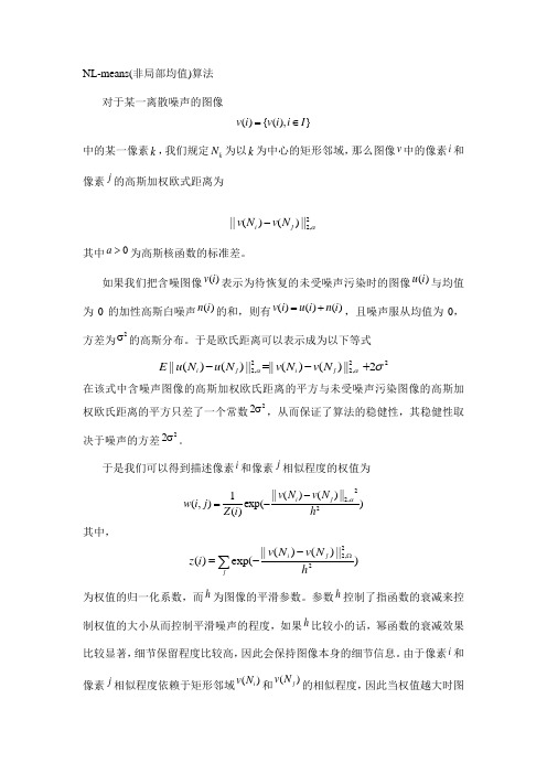
NL-means(非局部均值)算法对于某一离散噪声的图像(){(),}v i v i i I =∈中的某一像素k ,我们规定k N 为以k 为中心的矩形邻域,那么图像v 中的像素i 和像素j 的高斯加权欧式距离为2,2||)()(||αj i N v N v -其中0a >为高斯核函数的标准差。
如果我们把含噪图像()v i 表示为待恢复的未受噪声污染时的图像()u i 与均值为0的加性高斯白噪声()n i 的和,则有()()()v i u i n i =+,且噪声服从均值为0,方差为2σ的高斯分布。
于是欧氏距离可以表示成为以下等式22,22,22||)()(||||)()(||σαα+-=-j i j i N v N v N u N u E 在该式中含噪声图像的高斯加权欧氏距离的平方与未受噪声污染图像的高斯加权欧氏距离的平方只差了一个常数22σ,从而保证了算法的稳健性,其稳健性取决于噪声的方差22σ。
于是我们可以得到描述像素i 和像素j 相似程度的权值为22,2||()()||1(,)exp()()i j v N v N w i j Z i hα-=- 其中,∑Ω--=jj i hN v N v i z )||)()(||exp()(22,2为权值的归一化系数,而h 为图像的平滑参数。
参数h 控制了指函数的衰减来控制权值的大小从而控制平滑噪声的程度,如果h 比较小的话,幂函数的衰减效果比较显著,细节保留程度比较高,因此会保持图像本身的细节信息。
由于像素i 和像素j 相似程度依赖于矩形邻域()i v N 和()j v N 的相似程度,因此当权值越大时图像的矩形邻域就越相似。
同时,权值(,)w i j 还满足以下条件:0(,)1w i j ≤≤且(,)1w i j =∑。
下图(图1)为计算图像自身相似程度的例子,其中像素p 和像素1q 具有相似的矩形邻域,而像素p 和像素2q 的矩形邻域相似程度较低。
Parameter-Free Fast Pixelwise Non-Local Means Denoising
Parameter-Free Fast Pixelwise Non-Local Means Denoising
that the image denoising community has freely available a documented, verified and open-source implementation of NLM in its original version. Despite the number of NLM codes that can be found in the Internet, it seems that there are only two implementations that fulfill these conditions: the nlmeans module included in MegaWave2 [11] and written by Lionel Moisan and the IPOL article [4] from Buades, Coll and Morel. The first code implements the pixelwise NLM algorithm given in [1] (Section 5.1) for gray-level images only and using the Euclidean norm instead of the uniform one to define neighbor patches. The parameters’ default values correspond to those in [1], but they turn out to be non optimal for most images. Finally, this code does not implement any algorithmic trick or parallelization of computing, making it a slow running program. While the IPOL article [4] describes both the pixelwise NLM (NLM-P) ([1] Section 5.1) and the blockwise NLM (NLM-B) ([1] Section 5.5.2), the published demo and code implement the blockwise version only2 . The present article aims to propose a fast and parameter-free implementation of the pixelwise NLM as described in [1] (pages 510-512). In order to fix the notation, let us first recall the equations that lead to this algorithm. The input, noisy image v , is assumed to come from the classical additive noise model v (x) = u(x) + (x), x ∈ Ω, (1)
Fast-NLM
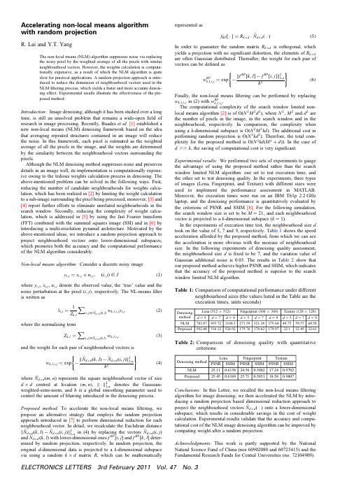
Accelerating non-local means algorithm with random projectioni and Y.T.YangThe non-local means (NLM)algorithm suppresses noise via replacing the noisy pixel by the weighted average of all the pixels with similar neighbourhood vectors.However,the weights calculation is computa-tionally expensive,as a result of which the NLM algorithm is quite slow for practical applications.A random projection approach is intro-duced to reduce the dimension of neighbourhood vectors used in the NLM filtering process,which yields a faster and more accurate denois-ing effect.Experimental results illustrate the effectiveness of the pro-posed method.Introduction:Image denoising,although it has been studied over a long time,is still an unsolved problem that remains a wide-open field of research in image processing.Recently,Buades et al.[1]established a new non-local means (NLM)denoising framework based on the idea that averaging repeated structures contained in an image will reduce the noise.In this framework,each pixel is estimated as the weighted average of all the pixels in the image,and the weights are determined by the similarity between the neighbourhood vectors surrounding the pixels.Although the NLM denoising method suppresses noise and preserves details in an image well,its implementation is computationally expens-ive owing to the tedious weights calculation process in denoising.The above-mentioned problem can be solved in the following ways.First,reducing the number of candidate neighbourhoods for weights calcu-lation,which has been realised in [2]by limiting the weight calculation to a sub-image surrounding the pixel being processed,moreover,[3]and [4]report further efforts to eliminate unrelated neighbourhoods in the search window.Secondly,reducing the complexity of weight calcu-lation,which is addressed in [5]by using the fast Fourier transform (FFT)combined with the summed squares image (SSI)and in [6]by introducing a multi-resolution pyramid architecture.Motivated by the above-mentioned ideas,we introduce a random projection approach to project neighbourhood vectors onto lower-dimensional subspaces,which promotes both the accuracy and the computational performance of the NLM algorithm considerably.Non-local means algorithm:Consider a discrete noisy imagey i ,j =x i ,j +n i ,j ,(i ,j )[I(1)where y i ,j ,x i ,j ,n i ,j denote the observed value,the ‘true’value and the noise perturbation at the pixel (i ,j ),respectively.The NL-means filter is written asˆxi ,j =1Z k ,l(i ,j )[ˆN d ×d (k ,l )w k ,l ,i ,j y i ,j (2)where the normalising termZ k ,l =(i ,j )[ˆNd ×d (k ,l )w k ,l ,i ,j(3)and the weight for each pair of neighbourhood vectors isw k ,l ,i ,j =exp −ˆN d ×d (k ,l )−ˆN d ×d (i ,j ) 22,ah 2(4)where ˆNd ×d (m ,n )represents the square neighbourhood vector of size d ×d centred at location (m ,n ), · 22,a denotes the Gaussian-weighted-semi-norm,and h is a global smoothing parameter used to control the amount of blurring introduced in the denoising process.Proposed method:To accelerate the non-local means filtering,we propose an alternative strategy that employs the random projection approach introduced in [7]to perform dimensional reduction for each neighbourhood vector.In detail,we recalculate the Euclidean distanceˆN d ×d (k ,l )−ˆN d ×d (i ,j ) 22,ain (4)by replacing the vectors ˆN d ×d (i ,j )and ˆNd ×d (k ,l )with lower-dimensional ones f RP [i ,j ]and f RP [k ,l ]deter-mined by random projection,respectively.In random projection,the original d -dimensional data is projected to a k -dimensional subspace via using a random k ×d matrix R ,which can be mathematicallyrepresented asf RP [·]=R k ×d ·ˆNd ×d (·)(5)In order to guarantee the random matrix R k ×d is orthogonal,whichyields a projection with no significant distortion,the elements of R k ×d are often Gaussian distributed.Thereafter,the weight for each pair of vectors can be defined asw RP k ,l ,i ,j =exp − f RP [k ,l ]−f RP[i ,j ] 22,ah 2(6)Finally,the non-local means filtering can be performed by replacingw k ,l ,i ,j in (2)with w RP k ,l ,i ,j .The computational complexity of the search window limited non-local means algorithm [2]is of O(N 2M 2d 2),where N 2,M 2and d 2are the number of pixels in the image,in the search window and in the neighbourhood,respectively.In comparison,the complexity when using a k -dimensional subspace is O(N 2M 2kd ).The additional cost in performing random projection is O(N 2kd 2).Therefore,the total com-plexity for the proposed method is O(N 2kd (M 2+d )).In the case of d ..k ,the saving of computational cost is very significant.Experimental results:We performed two sets of experiments to gauge the advantage of using the proposed method rather than the search window limited NLM algorithm:one set to test execution time,and the other set to test denoising quality.In the experiments,three types of images (Lena,Fingerprint,and Texture)with different sizes were used to implement the performance assessment in MATLAB.Moreover,the execution times were run on an IBM T61p 2.2GHz laptop,and the denoising performance is quantitatively evaluated by the criterions of PSNR and SSIM [8].For the following simulation,the search window size is set to be M ¼21,and each neighbourhood vector is projected to a k -dimensional subspace (k ¼1).In the experiments of execution time test,the neighbourhood size d took on the value of 5,7and 9,respectively.Table 1shows the speed acceleration afforded by the proposed method,from which we can see the acceleration is more obvious with the increase of neighbourhood size.In the following experiments of denoising quality assessment,the neighbourhood size d is fixed to be 7,and the variation value of Gaussian additional noise is 0.03.The results in Table 2show that our proposed method achieves higher PSNR and SSIM,which indicates that the accuracy of the proposed method is superior to the search window limited NLM algorithm.Table 1:Comparison of computational performance under differentneighbourhood sizes (the values listed in the Table are the execution times,units seconds)Table 2:Comparison of denoising quality with quantitativecriterionsConclusions:In this Letter,we recalled the non-local means filtering algorithm for image denoising;we then accelerated the NLM by intro-ducing a random projection based dimensional reduction approach toproject the neighbourhood vectors ˆNd ×d (·)onto a lower-dimensional subspace,which results in considerable savings in the cost of weight calculation.Experimental results validate that the accuracy and compu-tational cost of the NLM image denoising algorithm can be improved by computing weight after a random projection.Acknowledgments:This work is partly supported by the National Natural Science Fund of China (nos 60902080and 60725415)and the Fundamental Research Funds for Central Universities (no.72104909).ELECTRONICS LETTERS 3rd February 2011Vol.47No.3#The Institution of Engineering and Technology201116September2010doi:10.1049/el.2010.2618i and Y.T.Yang(Department of Microelectronics,Xidian University,Xi’an,People’s Republic of China)E-mail:rlai@References1Buades,A.,Coll,B.,and Morel,J.M.:‘A review of image denoising algorithms,with a new one’,Multiscale Model.Simul.SIAM Interdiscip.J.,2005,4,(2),pp.490–5302Buades,A.,Coll,B.,and Morel,J.M.:‘Denoising image sequences does not require motion estimation’.Proc.IEEE2005Int.Conf.Advanced Video and Signal Based Surveillance,Teatro Sociale,Italy,pp.70–74 3Mahmoudi,M.,and Sapiro,G.:‘Fast image and video denoising via nonlocal means of similar neighborhoods’,IEEE Signal Process.Lett., 2005,12,(12),pp.839–8424Orchard,J.,Ebrahimi,M.,and Wong,A.:‘Efficient non-local means denoising using the SVD’.Proc.2008IEEE Int.Conf.Image Processing,San Diego,CA,USA,pp.1732–17355Wang,J.,Guo,Y.W.,Ying,Y.T.,Liu,Y.L.,and Peng,Q.S.:‘Fast non-local algorithm for image denoising’.Proc.2006IEEE Int.Conf.Image Processing,Atlanta,GA USA,pp.1429–14326Karnati,V.,Uliyar,M.,and Dey,S.:‘Fast non-local algorithm for image denoising’.Proc.2008IEEE Int.Conf.Image Processing,San Diego, CA,USA,pp.3873–38767Bingham,E.,and Mannila,H.:‘Random projection in dimensional reduction:applications to image and text data’.Proc.2001ACM Int.Conf.Knowledge Discovery and Data Mining,San Francisco,CA, USA,pp.245–2508Wang,Z.,Bovik,A.C.,Sheikh,H.R.,and Simoncelli,E.P.:‘Image quality assessment:from error visibility to structural similarity’,IEEE Trans.Image Process.,2004,13,(4),pp.600–612ELECTRONICS LETTERS3rd February2011Vol.47No.3。
pmap anon的引用

pmap anon的引用英文回答:Shared Memory Allocation and Protection in the Linux Kernel: A Detailed Exploration of pmap_anon.In a multi-tasking operating system like Linux, one of the key challenges is managing memory effectively. This involves allocating memory to processes and ensuring that they do not interfere with each other's memory spaces. One important data structure in the Linux kernel that plays a crucial role in memory management is the Page Map, also known as pmap.The pmap_anon is a specific type of page map used to manage anonymous memory. Anonymous memory refers to memory that is not backed by any file or device, and is typically used for temporary allocations such as the heap or stack. Unlike file-backed memory, anonymous memory does not have a persistent presence on the disk and is allocateddynamically as needed.Mechanism and Implementation of pmap_anon.The pmap_anon is implemented as a radix tree, which isa specialized data structure optimized for efficient memory management. The radix tree is organized into levels, where each level represents a different bit position in thevirtual address. By using a combination of masks and shifts, the kernel can quickly traverse the tree and locate the appropriate page table entry for a given virtual address.Architecture and Key Functions.The pmap_anon is a complex data structure with several important functions:1. Memory Allocation: pmap_anon manages the allocationof anonymous memory pages. When a process requests memory, the kernel allocates a page from the free memory pool and adds it to the pmap_anon.2. Page Table Management: pmap_anon keeps track of the page table entries associated with each anonymous memory page. It ensures that the page tables are updated correctly when pages are allocated, deallocated, or moved.3. Protection and Permissions: pmap_anon enforces memory protection by setting the appropriate permissionsfor each page. It controls which processes have access to a particular page and what type of access (read, write, execute) they are allowed.4. Page Fault Handling: When a process accesses a page that is not in memory, the kernel triggers a page fault. pmap_anon plays a role in handling page faults by providing the necessary information to the kernel to resolve thefault and bring the page into memory.Performance Optimizations.To improve performance, the Linux kernel employs several optimizations related to pmap_anon. These optimizations include:1. Page Table Caching: The kernel caches page table entries to reduce the overhead of accessing page tables. When a process accesses a page, the kernel checks if the page table entry is cached. If it is, the kernel can avoid traversing the pmap_anon tree and directly access the page table entry.2. Large Page Support: The kernel supports the use of large pages, which are larger than the standard 4KB page size. Large pages improve performance by reducing the number of page table entries required and minimizing the overhead of page table management.中文回答:pmap_anon 在 Linux 内核中的引用,共享内存分配与保护。
长链非编码RNA在免疫系统调节中的作用
长链非编码RNA在免疫系统调节中的作用AbstractLong non-coding RNAs (lncRNAs) have recently emerged as key players in the regulation of immune response and are involved in diverse cellular processes. This review aims to provide an overview of the functions of lncRNAs in immunoregulation, including their roles in inflammatory response, immune cell differentiation and proliferation, and immune checkpoint regulation. Additionally, we discuss how lncRNAs may be involved in the development of immune-related diseases, such as autoimmune disorders and cancer. Improved understanding of the roles of lncRNAs in immune regulation will provide new opportunities to develop targeted therapies for a range of immune-related diseases.Keywords: Long non-coding RNA, Immunoregulation, Inflammatory response, Immune cell differentiation and proliferation, Immune checkpoint regulation, Autoimmune disorders, Cancer.摘要近年来,长链非编码RNA(lncRNA) 在免疫反应调节中已被证明是重要的调节因子,涉及多种细胞过程。
长链非编码RNA的调控机制及其在原发性肝癌中的研究进展
长链非编码RNA的调控机制及其在原发性肝癌中的研究进展常磊;刘志苏【摘要】Long non-coding RNA (lncRNA)has been a focal point of biomedical researches in recent years.Long noncoding RNAs (lncRNAs)are a class of transcripts of over 200 nucleotides with limited protein coding potential.Recent researches have shown that lncRNA played a key role in gene regulation.Some abnormally expressed lncRNAs could regulate gene expression at the levels of pre-transcription,transcription,post-transcription and epigenetics.This review summarized the biological characteristics,regulatory mechanisms and advances of hepatocellular carcinoma.%长链非编码 RNA(long non-coding RNA,lncRNA)是近年来生命科学领域研究的热点,它是指一类转录本长度超过200 nt 的非蛋白编码序列。
近年来的研究表明,lncRNA 具有基因调控的功能。
某些 lncRNA 在肿瘤中的表达也是失调的,可以在转录前、转录、转录后及表观遗传学等多个层面发挥作用,本文就lncRNA 生物学特点和调控机制及其在原发性肝癌中的研究进展作一综述。
【期刊名称】《腹部外科》【年(卷),期】2015(000)001【总页数】5页(P60-64)【关键词】长链非编码RNA;调控;原发性肝癌【作者】常磊;刘志苏【作者单位】430071 武汉,武汉大学中南医院肝胆胰外科;430071 武汉,武汉大学中南医院肝胆胰外科【正文语种】中文【中图分类】R657.3经典的中心法则“DNA-RNA-蛋白质”揭示基因的信息储存于编码蛋白质的基因组中。
非编码rna基因名词解释
非编码RNA(Non-Coding RNA,ncRNA)是指在细胞中转录而成的,但不编码蛋白质的RNA分子。
相对于编码蛋白质的mRNA(messenger RNA),ncRNA在过去被认为是"噪音"或"废物",但随着研究的深入,发现它们在细胞生物学中扮演着关键的角色。
以下是一些与非编码RNA相关的术语的解释:1.miRNA(MicroRNA):▪微小RNA,长度约为20-25个核苷酸,能够通过与mRNA结合,调控目标基因的表达。
它参与了许多生物学过程,如细胞周期调控、细胞分化和凋亡。
2.siRNA(Small Interfering RNA):▪小干扰RNA,与miRNA相似,也是长度约为20-25个核苷酸的RNA分子,主要通过RNA干扰途径抑制目标基因的表达。
它可以用于实验室研究中的基因沉默。
3.lncRNA(Long Non-Coding RNA):▪长非编码RNA,相对于miRNA和siRNA,lncRNA更长,一般指超过200个核苷酸。
lncRNA具有多样的功能,包括调控基因表达、染色体结构和细胞周期等。
4.piRNA(Piwi-Interacting RNA):▪Piwi相互作用RNA,是一类长度约为24-31个核苷酸的小RNA,主要与Piwi蛋白相互作用,参与调控生殖细胞发育和维护基因组稳定性。
5.snRNA(Small Nuclear RNA):▪小核RNA,主要存在于细胞核中,与蛋白质结合形成小核糖核蛋白颗粒,参与剪接体的形成和催化。
6.snoRNA(Small Nucleolar RNA):▪小核仁RNA,主要存在于细胞核仁中,参与核仁的形成和核糖体RNA的修饰。
7.circRNA(Circular RNA):▪环状RNA,是一类闭环结构的RNA分子,其结构相对稳定,具有较长的半衰期。
circRNA参与多种生物学过程,包括调控基因表达和作为miRNA的“海绵”调节miRNA的活性。
nonlocal注意力机制代码

nonlocal注意力机制代码非局部注意力机制(nonlocal attention mechanism)是一种用于计算机视觉任务的注意力机制,其目的是在一个图像或视频中建立全局的关联。
注意力机制旨在模拟人类视觉系统的特征提取过程。
在图像识别任务中,对于感兴趣的目标,并不是所有的细节都是重要的。
通过引入注意力机制,模型可以学习到对于不同部分的关注程度,从而引导模型更好地进行特征提取和分类。
传统的注意力机制主要关注局部区域,比如卷积神经网络(CNN)中的空间注意力机制(Spatial Attention)。
非局部注意力机制引入了全局性的信息交互,使得模型能够更好地捕捉到整体上的关联。
非局部注意力机制最早由王晓剑等人提出,并应用于视频分类任务。
以下是该方法的伪代码表示:```def NonLocalAttention(input, theta_weight, phi_weight, g_weight, output_weight):# 输入参数:# input: 输入特征图,shape为[N, C, H, W]# theta_weight, phi_weight, g_weight: 权重矩阵,shape为[N,C/2, C/2]# output_weight: 输出特征图的权重矩阵,shape为[N, C, H, W]# 1. 分离输入特征图为三个矩阵theta = Conv2d(input, theta_weight) # 使用卷积操作为其添加权重 theta_weight,得到 [N, C/2, H, W]phi = Conv2d(input, phi_weight) # 使用卷积操作为其添加权重 phi_weight,得到 [N, C/2, H, W]g = Conv2d(input, g_weight) # 使用卷积操作为其添加权重g_weight,得到 [N, C/2, H, W]# 2. 将 theta 和 phi 进行展开,并对应位置相乘,计算得到注意力图theta = Reshape(theta, [N, C/2, H*W]) # 将 theta 从 [N, C/2, H, W] 变形为 [N, C/2, H*W]theta = Transpose(theta, [0, 2, 1]) # 将维度 1 和 2 进行交换,得到 [N, H*W, C/2]phi = Reshape(phi, [N, C/2, H*W]) # 类似地,将 phi 变形为[N, C/2, H*W]f = Matmul(theta, phi) # 点乘操作,得到注意力图 [N, H*W,H*W]attention_map = Softmax(f, axis=2) # 对 f 进行 softmax 操作,以得到归一化的注意力图# 3. 用注意力图与 g 矩阵相乘,得到加权的输出特征图g = Reshape(g, [N, C/2, H*W]) # 将 g 变形为 [N, C/2, H*W]g = Transpose(g, [0, 2, 1]) # 将维度 1 和 2 进行交换,得到[N, H*W, C/2]y = Matmul(attention_map, g) # 将注意力图与 g 进行矩阵乘法操作,得到 [N, H*W, C/2]y = Reshape(y, [N, H, W, C/2]) # 将 y 变形为 [N, H, W, C/2] y = Transpose(y, [0, 3, 1, 2]) # 将维度 1 和 4 进行交换,得到[N, C/2, H, W]# 4. 将窗口大小为 1 的卷积应用于 y,得到最终的输出特征图output = Conv2d(y, output_weight) # 使用卷积操作为 y 添加权重 output_weight,得到 [N, C, H, W]return output```非局部注意力机制在视觉任务中取得了显著的性能提升。
ensrnop编号
ensrnop编号English Answer:ENSEMBL Transcript ID (ENST), also known as ENSEMBL Transcript Identification Number or ENSRNO, is a unique identifier assigned to each transcript model in the ENSEMBL database. It is a stable and versioned identifier that remains the same across ENSEMBL releases, allowing users to track and reference specific transcript models over time.ENSTs are composed of two parts:1. ENSEMBL Gene ID (ENSG): A stable and versioned identifier assigned to each gene model in the ENSEMBL database.2. Transcript version number: A numeric version number that indicates the specific version of the transcript model.ENSTs are typically used for the following purposes:Identifying and referencing specific transcript models in scientific publications and databases.Tracking changes and updates to transcript models over time.Performing comparative analyses of transcript models across different species or tissues.Developing and validating gene expression assays and other molecular biology techniques.中文回答:ENSEMBL 转录序列号 (ENST),也称为 ENSEMBL 转录序列识别号或 ENSRNO,是分配给 ENSEMBL 数据库中每个转录本模型的唯一标识符。
notch信号通路
notch配体
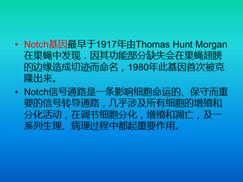
• 即,Delta/Serrate/LAG-2 (DSL)家族
• 在果蝇中Notch个配体为Delta和Serrate,线虫为Lag-2,取首写字母, Notch的配体又被称为DSL蛋白(在哺乳动物中叫做Jagged)
• 特点: • ①单次跨膜蛋白糖蛋白 • ②胞外有数量不等的EGF样重复区 • ③N 端有一个结合 Notch 受体必需的 DSL基序 • ④与Notch 受体不同的是, 配体分子的胞浆区很 • 短, 只有70~ 215个氨基酸残基. •
调节因子
• 胞外的Fringe蛋白(FNG)
•
抑制Delta和Serrate配体对Notch受体的激活
• 胞内的Deltex(Dtx)
• Numb蛋白——抑制notch信号
Notch信号的靶基因
• 多为碱性螺旋-环-螺旋类转录因子(basic helixloop-helix,bHLH)
• 它们又调节其它与细胞分化直接相关的基因的转 录。如哺乳动物中的HES(hairy/ enhancer of split)、果蝇中的E(spl) (enhancer of split) 及非洲爪蟾中的XHey-1,人类的Hes1,Hes5等。
• 哺乳动物中 ps、nieastrin、 Aph一l 和 pen 一2 四个膜蛋白在高尔基体中共同组装成有 活性的 Y - 分泌酶,催化 Notch 蛋 白水解。
• 认为 P S 是真正切割 Notch 的酶,而 nieastrin Aph一l 和 pen 一2可能通过修饰 ps酶或其底物来 调控γ-促分泌酶复合体酶 的活性
Notch 受体 异源二聚体 约300kb的蛋白
• 胞外亚单位(ECN)
• EGF样的重复片段 (EGF-R)
线粒体基因非编码区 -回复
线粒体基因非编码区-回复线粒体基因非编码区(Mitochondrial noncoding region)是线粒体DNA 中编码基因之外的区域,也被称为控制区或D-loop区。
本文将从概述线粒体基因非编码区的位置和特点开始,详细介绍其功能和重要性,最后探讨目前对该区域的研究进展。
线粒体基因非编码区位于线粒体DNA的5'端,包括了起始转录位点、重复序列、控制元件和维持线粒体DNA复制及转录的特殊结构。
基因非编码区的长度通常在1000至1500碱基对之间,但不同物种之间也存在差异。
该区域以高度保守亦或高度重复序列为特征,这使得它在进化中相对稳定。
线粒体基因非编码区具有重要的功能。
首先,该区域含有线粒体DNA的起始转录位点,通过在该位点上结合转录因子,启动线粒体转录过程,将DNA转录为RNA。
其次,基因非编码区包含了调控基因表达的控制元件,例如:启动子、调节序列和转录因子结合位点。
这些元件能够调节线粒体转录因子的结合与活性,影响基因的表达水平。
另外,该区域存在大量的重复序列,这些序列在复制过程中可能会导致错误的拷贝和插入事件,这进一步增加了基因组的变异性。
此外,基因非编码区还包含了控制线粒体DNA复制和拷贝数的重要结构。
线粒体基因非编码区对维持线粒体功能和整个细胞的代谢活动具有重要作用。
首先,该区域的控制元件调节线粒体基因的表达,影响线粒体蛋白质合成的水平。
线粒体蛋白质是维持细胞呼吸链和氧化磷酸化功能的关键分子。
其次,线粒体基因非编码区的结构特征使其容易受到环境因素和突变的影响,从而导致线粒体功能的异常和相关疾病。
最后,基因非编码区的变异对线粒体DNA复制和拷贝数的调控至关重要。
任何基因组的异常复制与拷贝均可能影响线粒体的数量和质量,从而损害整个细胞的正常代谢活动。
近年来,对线粒体基因非编码区的研究不断深入。
研究人员通过测序技术和生物信息学分析,揭示了该区域的序列特点、结构和功能调控元件。
另外,一些研究还进一步探索了基因非编码区与线粒体相关疾病的关联,并尝试通过改变基因的表达水平来治疗这些疾病。
线粒体基因非编码区
线粒体基因非编码区
非编码区域在线粒体基因组中占据了相当大的比例,虽然它们不编码蛋白质,但在线粒体功能和调控中扮演着重要的角色。
以下是一些关于线粒体基因非编码区的重要信息:
1. rRNA和tRNA基因,线粒体基因组中的非编码区域包含了编码线粒体rRNA和tRNA的基因。
这些基因在蛋白质合成和线粒体功能中起着至关重要的作用。
2. 控制元素,线粒体基因组的非编码区域还包含了许多控制元素,如启动子、增强子、转录因子结合位点等。
这些控制元素对于线粒体基因的转录和调控起着重要的作用。
3. 调控RNA,线粒体基因组的非编码区域还包含了一些调控RNA,如线粒体转运RNA(tRNA)和线粒体微小RNA(miRNA)。
这些调控RNA参与线粒体基因的表达调控和线粒体功能的调节。
4. 重组和突变,线粒体基因组的非编码区域也是重组和突变的热点区域。
由于线粒体基因组的特殊性质,非编码区域的重组和突变可能导致线粒体功能的改变,进而影响细胞的能量代谢和其他线
粒体相关的生理过程。
5. 进化研究,线粒体基因组的非编码区域也被广泛用于进化研究。
由于非编码区域的相对保守性较低,它们可以作为遗传变异和进化过程的标记,用于研究不同物种之间的亲缘关系和进化历史。
总之,线粒体基因组的非编码区域在线粒体功能和调控中具有重要作用。
它们包含了编码rRNA和tRNA的基因、控制元素、调控RNA以及参与重组和突变等。
研究非编码区域可以帮助我们更好地理解线粒体的功能和进化过程。
nldm原理
nldm原理NLDm原理——理解自然语言推理的奥秘自然语言推理(Natural Language Deduction,简称NLD)是人工智能领域中一项重要的任务,它旨在利用计算机对人类语言进行理解和推理。
而NLDm原理则是自然语言推理中的一种重要原理,它在推理过程中起到了至关重要的作用。
本文将从NLDm原理的定义、原理解析以及应用场景三个方面对其进行深入探讨。
一、NLDm原理的定义NLDm原理是指自然语言推理中的“非线性分布分解”原理。
简单来说,它是基于大规模语料库和机器学习算法,通过对语义信息的分析和推理,将自然语言中的句子进行理解和转化,从而实现对语义的推断和判断。
二、NLDm原理的原理解析NLDm原理的核心思想是将自然语言中的句子进行分布式表示,通过对句子的向量化,实现对语义信息的提取和分析。
在这个过程中,NLDm原理使用了一种非线性映射函数,将输入的句子映射到一个高维空间中,并通过计算句子之间的相似度,实现对语义信息的推理。
具体而言,NLDm原理包括以下几个步骤:1. 语料库建立:收集大规模的自然语言语料,构建一个包含丰富语义信息的语料库。
2. 句子向量化:利用词袋模型或者词嵌入等技术,将句子表示为向量形式,以便计算机可以对其进行处理。
3. 非线性映射:将句子的向量通过非线性映射函数转换为高维向量,以增强语义信息的表达能力。
4. 相似度计算:通过计算向量之间的相似度,判断句子之间的语义关系,包括蕴含、矛盾、中立等。
5. 推理判断:根据相似度计算的结果,进行推理判断,得出结论。
三、NLDm原理的应用场景NLDm原理在自然语言推理中有广泛的应用。
以下是几个典型的应用场景:1. 问答系统:利用NLDm原理可以对用户提出的问题进行语义分析和推理,从而给出准确的答案。
2. 文本分类:通过对文本进行向量化和相似度计算,可以将文本进行分类,实现信息的自动整理和归类。
3. 情感分析:利用NLDm原理可以对用户的情感进行分析和推断,从而实现情感分析和情感识别等功能。
- 1、下载文档前请自行甄别文档内容的完整性,平台不提供额外的编辑、内容补充、找答案等附加服务。
- 2、"仅部分预览"的文档,不可在线预览部分如存在完整性等问题,可反馈申请退款(可完整预览的文档不适用该条件!)。
- 3、如文档侵犯您的权益,请联系客服反馈,我们会尽快为您处理(人工客服工作时间:9:00-18:30)。
Non-Local Euclidean Medians Kunal N.Chaudhury and Amit SingerAbstract—In this letter,we note that the denoising performance of Non-Local Means(NLM)can be improved at large noise levels by replacing the mean by the Euclidean median.We call this new denoising algorithm the Non-Local Euclidean Medians(NLEM). At the heart of NLEM is the observation that the median is more robust to outliers than the mean.In particular,we provide a simple geometric insight that explains why NLEM performs better than NLM in the vicinity of edges,particularly at large noise levels. NLEM can be efficiently implemented using iteratively reweighted least squares,and its computational complexity is comparable to that of NLM.We provide some preliminary results to study the proposed algorithm and to compare it with NLM.Index Terms—Euclidean median,image denoising,non-local means,iteratively reweighted least squares(IRLS),Weiszfeld algorithm.I.I NTRODUCTIONN ON-LOCAL MEANS(NLM)is a data-driven diffusion mechanism that was introduced by Buades et al.in[1]. It has proved to be a simple yet powerful method for image denoising.In this method,a given pixel is denoised using a weighted average of other pixels in the(noisy)image.In par-ticular,given a noisy image,the denoised image at pixel is computed using the formula(1)where is some weight(affinity)assigned to pixels and. The sum in(1)is ideally performed over the whole image.In practice,however,one restricts to a geometric neighborhood of,e.g.,to a sufficiently large window of size[1]. The central idea in[1]was to set the weights using image patches centered around each pixel,namely as(2)Manuscript received July11,2012;revised August29,2012;accepted Au-gust30,2012.Date of publication September07,2012;date of current version September11,2012.The work of K.N.Chaudhury was supported in part by the Swiss National Science Foundation under Grant PBELP2-135867.The work of A.Singer was supported in part by the National Science Foundation under Award Award DMS-0914892,by the Air Force Office of Scientific Research under Award FA9550-09-1-0551,by the National Institute of General Medical Sciences under Award R01GM090200,and by the Alfred P.Sloan Foundation. The associate editor coordinating the review of this manuscript and approving it for publication was Prof.H.Vicky Zhao.K.N.Chaudhury is with the Program in Applied and Computational Math-ematics(PACM),Princeton University,Princeton,NJ08544USA(e-mail: kchaudhu@).A.Singer is with the PACM and Department of Mathematics,Princeton Uni-versity,Princeton,NJ08544USA(amits@).Digital Object Identifier10.1109/LSP.2012.2217329where and are the image patches of size centered at pixels and.Here,is the Euclidean norm of patch as a point in,and is a smoothing parameter.Thus,pixels with similar neighborhoods are given larger weights compared to pixels whose neighborhoods look different.The algorithm makes explicit use of the fact that repetitive patterns appear in most natural images.It is remarkable that the simple formula in (1)often provides state-of-the-art results in image denoising[2]. One outstanding feature of NLM is that,in comparison to other denoising techniques such as Gaussian smoothing,anisotropic diffusion,total variation denoising,and wavelet regularization, the so-called method noise(difference of the denoised and the noisy image)in NLM appears more like white noise[1],[2].We refer the reader to[2]for a detailed review of the algorithm. The rest of the letter is organized as follows.In Section II, we explain how the denoising performance of NLM can be im-proved in the vicinity of edges using the Euclidean median. Based on this observation,we propose a new denoising algo-rithm in Section III and discuss its implementation.This is fol-lowed by some preliminary denoising results in Section IV, where we compare our new algorithm with NLM.We conclude with some remarks in Section V.II.B ETTER R OBUSTNESS U SING E UCLIDEAN M EDIAN The denoising performance of NLM depends entirely on the reliability of the weights.The weights are,however,com-puted from the noisy image and not the clean image.Noise af-fects the distribution of weights,particularly when the noise is large.By noise,we will always mean zero-centered white Gaussian noise with variance in the rest of the discussion. To understand the effect of noise and to motivate the main idea of the paper,we perform a simple experiment.We con-sider the particular case where the pixel of interest is close to an(ideal)edge.For this,we take a clean edge profile of unit height and add noise to it.This is shown in Fig.1. We now select a point of interest a few pixels to the right of the edge(marked with a purple circle).The goal is to estimate its true value from its neighboring points using NLM.To do so,we take3-sample patches around each point,and a search window of.The patches are shown as points in3-di-mensions in Fig.2(a).The clean patch for the point of interest is at(1,1,1).We use(2)to compute the weights,where we set. The weights corresponding to the point of interest are shown in Fig.1(b).Using the noisy weights,we obtain an estimate of around0.65.This estimate has a geometric interpretation.It is the center coordinate of the Euclidean mean, where are the weights in Fig.1(b),and are the patches in Fig.2(a).The Euclidean mean is marked with a blue diamond in Fig.2.Note that the patches drawn from the search window are clustered around the centers and.1070-9908/$31.00©2012IEEEFig.1.Ideal edge in one dimension.(a)Clean and noisy edge.(b)Weights.Fig.2.Outlier model of the patch space for the point of interest in Fig.1(a).Due to its robustness to outliers,the Euclidean median behaves as a better estimator of the clean patch than the Euclidean mean (see text for explanation).(a)3d patch space close to the edge.(b)2d projection (first 2coordinates).For the point of interest,the points around are the outliers,while the ones around are the inliers.The noise reduces the relative gap in the corresponding weights,causing the mean to drift away from the inliers toward the outliers.Note that the Euclidean mean is the minimizer ofover all patches .Our main observation isthat,if we instead compute the minimizer ofover all ,and take the center coordinate of ,then we get a much better estimate.Indeed,the denoised value turns out to be around 0.92in this case.The above minimizer is called the Euclidean median (or the geometric median)in the literature [3].We will often simply call it the median.We repeated the above experiment using several noise realizations,and consistently got better results using the median.Averaged over 10trials,the denoised value using the mean and median were found to be 0.62and 0.93,respectively.Indeed,in Fig.2,note how close the median is to the true patch compared to the mean.This does not come as a surprise since it is well-known that the median is more robust to outliers than the mean.This fact has a rather simple explanation in one dimension.In higher dimensions,note that the former is the minimizer of the weighted norm of the distances ,while the latter is the minimizer of the weighted norm of these distances.It is this use of the norm over the norm that makes the Euclidean median more robust to outliers [3].III.N ON -L OCAL E UCLIDEAN M EDIANSFollowing the above observation,we propose Algorithm 1below which we call the Non-Local Euclidean Medians(NLEM).We use to denote the search window of sizecentered at pixel .Algorithm 1Non-Local Euclidean Medians Input :Noisy image,and parameters.Return :Denoised image.(1)Extract patch of size at every pixel .(2)For every pixel ,do (a)Set for every .(b)Find patch that minimizes.(c)Assign the value of the center pixel in .The difference with NLM is in step which involves the computation of the Euclidean median.That is,given pointsand weights ,we are required tofind that minimizes the convex cost .There exists an extensive literature on the computation of the Euclidean median;cf.[4],[5]and references therein.The sim-plest algorithm in this area is the so-called Weiszfeld algorithm [4],[5].This is,in fact,based on the method of iteratively reweighted least squares (IRLS),which has received renewed interest in the compressed sensing community in the context of minimization [6],[7].Starting from an estimate ,the idea is to set the next iterate asThis is a least-squares problem,and the minimizer is given by(3)where .Starting with an initial guess,one keeps repeating this process until convergence.In practice,one needs to address the situation when gets close to some ,which causes to blow up.In the Weiszfeld algorithm,one keeps track of proximity ofto all the ,and is set to be if for some .It has been proved by many authors that the iterates converge globally,and even linearly (exponentially fast)under certain conditions,e.g.,see discussion in [5].Following the recent ideas in [6],[7],we have also tried reg-ularizing (3)by adding a small bias,namely by setting.The bias is updated at each it-erate,e.g.,one starts with and gradually shrinks tozero as the iteration progresses.The convergence properties of a particular flavor of this algorithm are discussed in [7].We have tried both the Weiszfeld algorithm and the one in [6].Exper-iments show us that faster convergence is obtained using the latter,typically within 3to 4steps.The overall computational complexity of NLEM is per pixel,whereis the average number of IRLS iterations.The complexity of the standard NLM is per pixel.For example,for a 256256image,the typical run time of a C implementation of NLM was about 10seconds,and that forCHAUDHURY AND SINGER:NON-LOCAL EUCLIDEAN MEDIANS747Fig.3.Synthetic grayscale test images,original size 256256.Black is at intensity 0,and white is at intensity 255.(a)Checker .(b)Circles.Fig.4.The “”symbol marks pixels where the estimate returned by NLEMis signi ficantly better than that returned by NLM.(a)Checker.(b)House.NLEM was about 32seconds (on an Intel quad-core 2.83GHzmachine).IV .E XPERIMENTSWe now present the result of some preliminary denoising ex-periments.For this,we have used the synthetic images shown in Fig.3and some natural images.For NLEM,we computed the Euclidean median using the simple IRLS scheme described in [6].For all experiments,we have set ,andfor both algorithms.These are the standard settingsoriginally proposed in [1].First,we considered the Checker image.We added noise withresulting in a Peak-Signal-to-Noise Ratio (PSNR)of8.18dB.The PSNR improved to 17.94dB after applying NLM,and with NLEM this further went up to 19.45dB (averaged over 10noise realizations).This 1.5dB improvement is perfectly explained by the arguments provided in Section II.Indeed,in Fig.4(a),we have marked those pixels where the estimate from NLEM is signi ficantly closer to the clean image than that ob-tained using NLM.More precisely,denote the original image by ,the noisy image by ,and the denoised images from NLM and NLEM by and .Then the “”in the figure denotes pixels where .Note that these points are concentrated around the edges where the median performs better than the mean.So what happens when we change the noise level?We went fromto in steps of 10.The plots of the cor-responding PSNRs are shown in Fig.5(a).At low noise levelsparison of denoising performance for the Checker image at noise.NLM-kNN and NLEM-kNN refer to the respective modi fications ofNLM and NLEM where we use only the largest 50%of the weights.TABLE IC OMPARISON OF NLM AND NLEM IN T ERMS OF PSNR AND SSIM,AT N OISE L EVELS (A VERAGED O VER10N OISE R EALIZATIONS ).S AME P ARAMETERS U SED :,AND ,we see that NLM performs as good or even better thanNLEM.This is because at low noise levels the true neighbors in patch space are well identi fied,at least in the smooth regions.The difference between them is then mainly due to noise,and since the noise is Gaussian,the least-squares approach in NLM gives statistically optimal results in the smooth regions.On the other hand,at low noise levels,the two clusters in Fig.2are well separated and hence the weights for NLM are good enough to push the mean towards the right cluster.The median and mean in this case are thus very close in the vicinity of edges.At higher noise levels,the situation completely reverses and NLEM per-forms consistently better than NLM.In Fig.5(a),we see that this phase transition occurs at around .The improvement in PSNR is quite signi ficant beyond this noise level,as large as 2.1dB.The exact PSNRs are given in Table I.Next,we tried the above experiment on the Circles image.The results are given in Table I.The phase transition in this case occurs around .As in the previous case,NLEM performs better beyond the phase transition,and the gain in PSNR over NLM is as large as 2.2dB.The method noise for NLM and NLEM obtained from a typical denoising experiment are shown748IEEE SIGNAL PROCESSING LETTERS,VOL.19,NO.11,NOVEMBER2012parison of the method noise for the Circles image at. in Fig.6.Note that the method noise for NLEM appears more white(with less structural features)than that for NLM. Finally,we considered some benchmark natural images, namely House,Barbara,and Lena.The PSNRs obtained from NLM and NLEM for these images at different noise levels are shown in Table I.The table also compares the Structural Similarity(SSIM)indices[12]obtained from the two methods. Note that a phase transition in SSIM is also observed for some of the images.In Fig.4(b),we show the pixels where NLEM does better(in the sense defined earlier)than NLM for the House image at.We again see that these pixels are concentrated around the edges.The improvements in PSNR and SSIM are quite dramatic for the synthetic images Checker and Circles.This is expected be-cause they contain many edges and the edges have large tran-sitions.The improvement in PSNR and SSIM are less dramatic for the natural images.But,considering that NLM already pro-vides top quality denoising results,this small improvement is already significant.We have also noticed that the performance of NLEM(and that of NLM)can be further improved by consid-ering only the top50%of the-neighbors with largest weights in step of Algorithm1.This simple modification improves both NLM and NLEM(and also their running time),while still maintaining their order in terms of PSNR performance.A com-parison of the four different methods is given in Fig.5(b).While we have considered afixed setting for the parameters,our gen-eral observation based on extensive experiments is that NLEM consistently performs better than NLM beyond the phase tran-sition,irrespective of the parameter settings.In future,we plan to investigate ways of further improving NLEM,and study the effect of the parameters on its denoising performance.V.D ISCUSSIONThe purpose of this note was to communicate the idea that one can improve(often substantially)the denoising results of NLM by replacing the regression on patch space by the more robust regression.This led us to propose the NLEM algo-rithm.The experimental results presented in this paper reveal two facts:(a)Phase transition phenomena—NLEM starts to per-form better(in terms of PSNR)beyond a certain noise level, and(b)The bulk of the improvement comes from pixels close to sharp edges.The latter fact indicates that NLEM is better suited for denoising images that have many sharp edges.This suggests that we could get similar PSNR improvements if we simply used NLEM in the vicinity of edges and the less expen-sive NLM elsewhere.Unfortunately,it is difficult to get a reli-able edge map from the noisy image.On the other hand,obser-vation(b)suggests that,by comparing the denoising results of NLM and NLEM,one can devise a robust method of detecting edges at large noise levels.We note that Wang et al.have re-cently proposed a non-local median-based estimator in[9].This can be considered as a special case of NLEM corresponding to ,where single pixels(instead of patches)are used for the median computation.On the other hand,some authors have pro-posed median-based estimators for NLM where the noisy image is medianfiltered before computing the weights[8],[9].In fact, most of the recent innovations in NLM were concerned with better ways of computing the weights;e.g.,see[10],[11],and references therein.It would be interesting to see if the idea of regression could be used to complement these innovations.R EFERENCES[1]A.Buades,B.Coll,and J.M.Morel,“A review of image denoisingalgorithms,with a new one,”Multiscale Model.Simul.,vol.4,pp.490–530,2005.[2]A.Buades,B.Coll,and J.M.Morel,“Image denoising methods.Anew nonlocal principle,”SIAM Rev.,vol.52,pp.113–147,2010.[3]P.J.Huber and E.M.Ronchetti,“Robust Statistics,”in Wiley Series inProbability and Statistics.Hoboken,NJ:Wiley,2009.[4]E.Weiszfeld,“Sur le point par lequel le somme des distances depoints donnes est minimum,”Tôhoku Math.J.,vol.43,pp.355–386,1937.[5]G.Xue and Y.Ye,“An efficient algorithm for minimizing a sumof Euclidean norms with applications,”SIAM J.Optim.,vol.7,pp.1017–1036,1997.[6]R.Chartrand and Y.Wotao,“Iteratively reweighted algorithms forcompressive sensing,”in IEEE ICASSP,2008,pp.3869–3872.[7]I.Daubechies,R.Devore,M.Fornasier,and C.S.Gunturk,“Iterativelyreweighted least squares minimization for sparse recovery,”Commun.Pure Appl.Math.,vol.63,pp.1–38,2009.[8]C.Chung,R.Fulton,D.D.Feng,and S.Meikle,“Median non-localmeansfiltering for low SNR image denoising:Application to PET withanatomical knowledge,”in IEEE Nuclear Science Symp.Conf.Rec.,2010,pp.3613–3618.[9]Y.Wang,A.Szlam,and G.Lerman,“Robust locally linear analysiswith applications to image denoising and blind inpainting,”submittedfor publication..[10]T.Tasdizen,“Principal neighborhood dictionaries for non-localmeans image denoising,”IEEE Trans.Image Process.,vol.18,pp.2649–2660,2009.[11]D.Van De Ville and M.Kocher,“Nonlocal means with dimensionalityreduction and SURE-based parameter selection,”IEEE Trans.ImageProcess.,vol.20,pp.2683–2690,2011.[12]Z.Wang,A.C.Bovik,H.R.Sheikh,and E.P.Simoncelli,“Imagequality assessment:From error visibility to structural similarity,”IEEETrans.Image Process.,vol.13,no.4,pp.600–612,2004.。
