Forecasting
cpfr的实施步骤有哪些

CPFR的实施步骤什么是CPFRCPFR,即合作伙伴资源计划(Collaborative Planning, Forecasting and Replenishment),是一种通过供应链合作来实现共同计划、预测和补货的方法。
CPFR致力于通过整合各方信息和资源,提高供应链的效率和灵活性,实现共赢。
CPFR的实施步骤CPFR的实施涉及多个步骤,以下是常见的实施步骤:1.建立合作伙伴关系–寻找合适的供应链合作伙伴,包括供应商、零售商和物流服务提供商。
–确定合作伙伴的权责,明确各方的角色和职责。
2.信息共享–在合作伙伴之间建立数据共享渠道,确保实时、准确的信息流动。
–共享的信息包括销售数据、库存数据、库存周转率等。
3.需求计划–基于历史数据和市场趋势,进行需求计划的预测。
–利用统计模型、市场调研等方法,预测未来的需求情况。
4.共同计划–基于需求计划,合作伙伴共同制定销售计划和生产计划。
–考虑到各方的资源和能力,制定合理的计划。
5.补货计划–根据销售计划和生产计划,制定补货计划。
–考虑到交货时间、库存水平等因素,优化补货计划。
6.执行补货–根据补货计划,各方执行补货操作。
–包括采购订单的生成、生产任务的下达等。
7.监控和反馈–监控补货执行情况,及时反馈问题和异常情况。
–根据监控结果,进行调整和改进。
8.持续改进–基于实际情况,对CPFR流程进行评估和改进。
–分析效果、问题和改进点,持续提升CPFR的效率和效果。
以上是CPFR的常见实施步骤,实际的实施过程中可能会因组织的特点而有所变化。
CPFR的实施需要合作伙伴之间的信任和配合,同时也需要合适的技术支持来实现信息共享和系统集成。
CPFR的成功实施可以提高供应链效率,减少库存和运营成本,并增强市场反应能力,提升客户满意度。
预测(Forecasting)
预测的定义预测(forecasting)是预计未来事件的一门艺术,一门科学。
它包含采集历史数据并用某种数学模型来外推与将来。
它也可以是对未来的主观或直觉的预期。
它还可以是上述的综合,即经由经理良好判断调整的数学模型。
进行预测时,没有一种预测方法会绝对有效。
对一个企业在一种环境下是最好的预测方法,对另一企业或甚至本企业内另一部门却可能完全不适用。
无论使用何种方法进行预测,预测的作用也是有限的,并不是完美无缺。
但是,几乎没有一家企业可以不进行预测而只是等到事情发生时再采取行动,一个好的短期或长期的经营规划取决于对公司产品需求的预测。
[编辑]预测的类型按在规划未来业务方面企业使用可分三种类型的预测:经济预测(economic forecasts)、技术预测(technological forecasts)、需求预测(demand forecasts)。
1、经济预测(economic forecasts),通过预计通货膨胀率、货币供给、房屋开工率及其它有关指标来预测经济周期。
2、技术预测(technological forecasts),即预测会导致产生重要的新产品,从而带动新工厂和设备需求的技术进步。
3、需求预测(demand forecasts),为公司产品或服务需求预测。
这些预测,也叫销售预测,决定公司的生产、生产能力及计划体系,并使公司财务、营销、人事作相应变动。
按它包含的时间跨度来分类,也有三种分类:短期预测、中期预测、长期预测1、短期预测。
短期预测时间跨度最多为1年,而通常少于3个月。
它用于购货、工作安排、所需员工、工作指定和生产水平的计划工作。
2、中期预测。
中期预测的时间跨度通常是从3个月到3年。
它用于销售计划、生产计划和预算、现金预算和分析不同作业方案。
3、长期预测。
长期预测的时间跨度通常为3年及3年以上。
它用于规划新产品、资本支出、生产设备安装或天职,及研究与发展。
中期预测和长期预测与短期预测的区别主要体现在以下三个方面:第一,中长期预测要处理更多的综合性问题并主要为产品、工厂、工序的管理决策提供支持;第二,短期预测采用的方法通常与长期预测采用的方法不同。
Forecasting

ForecastingWhy forecast?Features Common to all Forecasts∙Conditions in the past will continue in the future∙Rarely perfect∙Forecasts for groups tend to be more accurate than forecasts for individuals ∙Forecast accuracy declines as time horizon increasesElements of a Good Forecast∙Timely∙Accurate∙Reliable (should work consistently)∙Forecast expressed in meaningful units∙Communicated in writing∙Simple to understand and useSteps in Forecasting Process∙Determine purpose of the forecast∙Establish a time horizon∙Select forecasting technique∙Gather and analyze the appropriate data∙Prepare the forecast∙Monitor the forecastTypes of Forecasts∙Qualitativeo Judgment and opiniono Sales forceo Consumer surveyso Delphi technique∙Quantitativeo Regression and Correlation (associative)o Time seriesForecasts Based on Time Series Data∙What is Time Series?∙Components (behavior) of Time Series datao Trendo Cycleo Seasonalo Irregularo Random variationsNaïve MethodsNaïve Forecast – uses a single previous value of a time series as the basis of a forecast.Techniques for Averaging∙What is the purpose of averaging?∙Common Averaging Techniqueso Moving Averageso Exponential smoothingMoving AverageExponential SmoothingTechniques for TrendLinear Trend Equationline the of slope at of value pe riod time for fore cast from pe riods time of numbe r spe cifie d =====b ty a ty t t where t t 0:Curvilinear Trend Equationline the of slope at of value pe riod time for fore cast from pe riods time of numbe r spe cifie d =====b ty a ty t t where t t 0:Techniques for Seasonality∙ What is seasonality?∙ What are seasonal relatives or indexes?∙ How seasonal indexes are used:o Deseasonalizing datao Seasonalizing data∙ How indexes are computed (see Example 7 on page 109)Accuracy and Control of ForecastsMeasures of Accuracyo Mean Absolute Deviation (MAD)o Mean Squared Error (MSE)o Mean Absolute Percentage Error (MAPE) Forecast Control Measureo Tracking SignalMean Absolute Deviation (MAD)Mean Squared Error (or Deviation) (MSE)Mean Square Percentage Error (MAPE)Tracking SignalProblems:2 – Plot, Linear, MA, exponential Smoothing5 – Applying a linear trend to forecast15 – Computing seasonal relatives17 – Using indexes to deseasonalize values26 – Using MAD, MSE to measure forecast accuracyProblem 2 (110)National Mixer Inc., sells can openers. Monthly sales for a seven-month period were as follows:(a) Plot the monthly data on a sheet of graph paper.(b) Forecast September sales volume using each of the following:(1) A linear trend equation(2) A five-month moving average(3) Exponential smoothing with a smoothing constant equal to 0.20, assuming March forecast of19(000)(4) The Naïve Approach(5) A weighted average using 0.60 for August, 0.30 for July, and 0.10 for June(c) Which method seems least appropriate? Why?(d) What does use of the term sales rather than demand presume?EXCEL SOLUTION(a) Plot of the monthly dataHow to superimpose a trend line on the graph∙Click on the graph created above (note that when you do this an item called CHART will appear on the Excel menu bar)∙Click on Chart > Add Trend Line∙Click on the most appropriate Trend Regression Type∙Click OK(b) Forecast September sales volume using:(1) Linear Trend Equation∙Create a column for time period (t) codes (see column B)∙Click Tools > Data Analysis > Regression∙Fill in the appropriate information in the boxes in the Regression box that appearsCoded time periodSales dataCoded time period(2) Five-month moving average(3) Exponential Smoothing with a smoothing constant of 0.20, assuming March forecast of 19(000)∙Enter the smoothing factor in D1∙Enter “19” in D5 as forecast for March∙Create the exponential smoothing formula in D6, then copy it onto D7 to D11(4) The Naïve Approach(5) A weighted average using 0.60 for August, 0.30 for July, and 0.10 for JuneProblem 5 (110)A cosmetics manufactur er’s marketing department has developed a linear trend equation that can be used to predict annual sales of its popular Hand & Foot Cream.y t =80 + 15 twhere: y t = Annual sales (000 bottles) t0 = 1990(a) Are the annual sales increasing or decreasing? By how much?(b) Predict annual sales for the year 2006 using the equationProblem 15 (113)Obtain estimates of daily relatives for the number of customers at a restaurant for the evening meal, given the following data. (Hint: Use a seven-day moving average)Excel Solution∙Type a 7-day average formula in E6 ( =average(C3:c9) )∙In F6, type the formula =C6/E6∙Copy the formulas in E6 and F6 onto cells E7 to E27∙Compute the average ratio for Day 1 (see formula in E12)∙Copy and paste the formula in E12 onto E13 to E18 to complete the indexes for Days 2 to 7Problem 17 (113) – Using indexes to deseasonalize valuesNew car sales for a dealer in Cook County, Illinois, for the past year are shown in the following table, along with monthly (seasonal) relatives, which are supplied to the dealer by the regional distributor.(a) Plot the data. Does there seem to be a trend?(b) Deseasonalize car sales(c) Plot the deseasonalized data on the same graph as the original data. Comment on the two graphs.Excel Solution(a) Plot of original data (seasonalized car sales)(b) Deseasonalized Car Sales(c) Graph of seasonalized car sales versus deseasonalized car salesProblem 26 (115) – Using MAD, MSE, and MAPE to measure forecast accuracyTwo different forecasting techniques (F1 and F2) were used to forecast demand for cases of bottled water. Actual demand and the two sets of forecasts are as follows:(a) Compute MAD for each set of forecasts. Given your results, which forecast appears to be the mostaccurate? Explain.(b) Compute MSE for each set of forecasts. Given your results, which forecast appears to be the mostaccurate? Explain.(c) In practice, either MAD or MSE would be employed to compute forecast errors. What factors might leadyou to choose one rather than the other?(d) Compute MAPE for each data set. Which forecast appears to be more accurate?Excel Solution。
Chap2( Forecasting )2013-03-28(第5周 )
Southeast University
Dept. of Industrial Engineering
4
The Time Horizon in Forecasting The long term is measured in months or years; It is one part of the overall firm’s manufacturing strategy; Problems for long term forecasting include long term planning of capacity needs; long term sales patterns, and growth trend.
a phenomenon is some function of some variables
Objective-derived from analysis of data
Time Series Methods-forecast
of future values of some economic or physical phenomenon is derived from a collection of their past observations
Production Planning and Control
Chapter Two Forecasting
Department of Industrial Engineering Southeast University
Southeast University
Dept. of Industrial Engineering
1
Chapter Two
Forecasting
Forecasting
Business Forecaห้องสมุดไป่ตู้ting
The second possibility, management services, suffers from some of the problems of the data processing unit in being remote from the decision taking. Yet when the forecasts are for strategic decisions at board level this solution can be successful.
Business Forecasting
Forecasting is the process of using past events to make systematic predictions about future outcomes or trends. An observation popular with many forecasters is that “the only thing certain about a forecast is that it will be wrong.” Beneath the irony, this observation touches on an important point:
Business Forecasting
Introduction: Structure
The use of forecasting:
Managers must try to predict future conditions so that their goals and plans are realistic.
pytorch-forecasting deepar 用法-概述说明以及解释
pytorch-forecasting deepar 用法-概述说明以及解释1.引言1.1 概述时间序列预测是一种重要的数据分析技术,它在各种领域中都得到了广泛的应用,例如金融预测、销售预测、天气预测等。
随着深度学习的发展,越来越多的基于神经网络的模型被应用于时间序列预测问题中。
PyTorch是一个流行的深度学习框架,它提供了丰富的工具和库,用于构建和训练神经网络模型。
其中,pytorch-forecasting是基于PyTorch 开发的一个用于时间序列预测的库,它提供了多种强大的算法和模型,用于解决不同类型的时间序列预测问题。
在pytorch-forecasting库中,deepar算法是其中一个被广泛应用的模型。
deepar算法基于深度学习的思想,通过引入递归神经网络和自回归机制,可以对时间序列数据进行连续的预测,并且能够捕捉到数据中的隐藏模式和周期性。
本文将对pytorch-forecasting库和deepar算法进行详细介绍。
首先,我们将对pytorch-forecasting库进行简介,包括其特点、使用方法和相关工具。
然后,我们将深入探讨deepar算法的原理和关键概念。
接着,我们将介绍deepar算法在时间序列预测中的应用场景,并分析其优势和适用性。
最后,我们将具体讲解deepar算法的使用方法,包括数据准备、模型构建、训练和预测等步骤。
通过本文的学习,读者将能够了解pytorch-forecasting库和deepar 算法的基本原理和使用方法,并且掌握如何应用这些技术解决实际的时间序列预测问题。
此外,我们还将对pytorch-forecasting的deepar算法进行评价,并提出可能的改进方向,以期进一步提升其预测性能和应用范围。
1.2 文章结构本文将详细介绍pytorch-forecasting deepar 的用法和应用。
文章分为三大部分:引言、正文和结论。
在引言部分,我们将首先概述本文要探讨的主题,并介绍pytorch-forecasting deepar 的背景和意义。
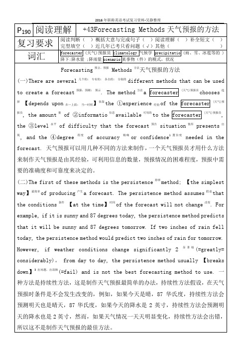
P190阅读理解43Forecasting Methods天气预报的方法
预示
. The method 方法 a forecaster (天气)预报员 chooses 选择
经验
】依靠 the ①experience
of the forecaster (天气)预报员,
the amount 量 of ②informatio 信息 available 可用的 to the forecaster (天气)预报员, the ③ level 水平 of difficulty that the forecast 预告 situation 情形 presents 出现, and the ④degree
Forecasting 预言,预报 Methods 方法天气预报的方法 (一)There are several 几个的;
专有的; 各自的; 分别的
different methods that can be used
to create a forecast 预报,预测; 【depends upon
在…上面; 当…时候
2016 年职称英语考试复习资料-吴静整理
P190 阅读理解 +43Forecasting Methods 天气预报的方法 阅读判断( )概括大意与完成句子( )阅读理解( )补全短文( ) 复习要求 完型填空( )近几年已考只看问题(√)其他( ) forecaster (天气)预报员 climatology 气候学 precipitatio (雨、雪、冰雹等的 ) 词汇 降下:降水量 ;降雨量 scenario 某事物(件)的模式,状况
weather in this forecast will behave the same as it did in the past. The analog method is difficult to use because it is virtually to find a predict analog. Various 各种各样的;
Forecasting

“Prediction is very difficult, especially if it's about the future.”
Nils Bohr
Objectives
• Give the fundamental rules of forecasting
• Calculate a forecast using a moving average, weighted moving average, and exponential smoothing • Calculate the accuracy of a forecast
Actual demand (past sales) Predicted demand
What’s Forecasting All About?
From the March 10, 2006 WSJ:
Ahead of the Oscars, an economics professor, at the request of Weekend Journal, processed data about this year's films nominated for best picture through his statistical model and predicted with 97.4% certainty that "Brokeback Mountain" would win. Oops. Last year, the professor tuned his model until it correctly predicted 18 of the previous 20 best-picture awards; then it predicted that "The Aviator" would win; "Million Dollar Baby" won instead.
international journal of forecasting 发表记

international journal of forecasting 发表记摘要:一、引言1.介绍“吃完饭后,你会做什么?”这个问题2.引入“吃完饭后,你会做什么?”的英文表达二、讲解“吃完饭后,你会做什么?”的英文表达1.讲解“吃完饭后,你会做什么?”的英文表达:What will you do after you"ve finished the meal?2.讲解“吃完饭后,你会做什么?”的英文表达:What do you usually do after you finish the meal?三、讲解“吃完饭后,你会做什么?”的英文表达1.讲解“吃完饭后,你会做什么?”的英文表达:Are there any other activities you like to do after finishing a meal?2.讲解“吃完饭后,你会做什么?”的英文表达:What are some common activities people do after they finish eating?四、总结1.总结“吃完饭后,你会做什么?”的英文表达2.强调学习“吃完饭后,你会做什么?”的英文表达的重要性正文:一、引言“吃完饭后,你会做什么?”这是一个日常生活中非常常见的问题。
然而,在英语中,我们该如何表达这个问题呢?今天,我们将学习如何用英语询问和回答这个问题。
二、讲解“吃完饭后,你会做什么?”的英文表达1.首先,让我们来学习一个直接的表达方式:“吃完饭后,你会做什么?”在英语中可以表达为:“What will you do after you"ve finished the meal?”这个句子可以用来询问别人在吃完饭后的计划。
2.另外,我们也可以使用一个更口语化的表达:“吃完饭后,你会做什么?”可以变成:“What do you usually do after you finish the meal?”这个句子适用于询问别人平时的习惯。
专业英语气象科技英语第三课 气象预报

Serve as 充当,作为
P1①National Meteorological Services perform a variety of activities in order to provide weather forecasts. ②The principal ones are data collection, the preparation of basic analyses and prognostic charts of short-and long-term forecasts for the public as well as special services for aviation, shipping , agricultural and other commercial and industrial users, and the issuance of severe weather warnings.
stations for severe weather . ②Under the World
Weather Watch (WWW) program, synoptic reports are made at some 4,000 land stations and by 7,000
ships. ③There are about 700 stations making
P7: During the first half of the century, short-range forecasts were based on synoptic principles, empirical rules and extrapolation of pressure changes.
工程项目财务管理的英语

Project financial management is a critical aspect of any construction or engineering project. It involves the planning, organizing, directing, and controlling of financial resources to ensure that the project is completed within budget, on time, and with the desired quality. In this article, we will explore the key components and challenges of project financial management in English.1. Budgeting and ForecastingThe first step in project financial management is to create a comprehensive budget. This includes estimating the costs of labor, materials, equipment, and other resources required for the project. Accurate budgeting is essential to ensure that the project does not exceed its financial limits.Forecasting is another important aspect of financial management. It involves predicting future financial performance based on historical data and market trends. By regularly reviewing and updating forecasts, project managers can make informed decisions and adjust the budget as necessary.2. Cost ControlCost control is a crucial component of project financial management. It involves monitoring and managing the costs associated with the project to ensure that they stay within the budget. This includes identifying cost overruns, analyzing the reasons behind them, and implementing corrective actions.Key strategies for cost control include:- Regularly reviewing project expenses against the budget.- Implementing cost-saving measures, such as negotiating better prices for materials and services.- Conducting variance analysis to identify deviations from the budget and take corrective action.3. Cash Flow ManagementEffective cash flow management is vital for the success of a project. It involves ensuring that the project has enough cash on hand to cover its expenses and maintain its operations. This includes:- Forecasting cash inflows and outflows.- Managing payment terms with suppliers and clients.- Implementing measures to improve liquidity, such as short-term loans or lines of credit.4. Risk ManagementFinancial risk management is essential in project management. It involves identifying, assessing, and mitigating financial risks that could impact the project's success. Common financial risks include:- Market fluctuations affecting material prices.- Delays in project completion leading to increased costs.- Unexpected legal or regulatory changes.To manage these risks, project managers can:- Develop contingency plans to address potential issues.- Purchase insurance to protect against financial losses.- Regularly review and update risk management strategies.5. Financial Reporting and AnalysisRegular financial reporting and analysis are essential for monitoring the project's financial health. This includes:- Preparing financial statements, such as balance sheets, income statements, and cash flow statements.- Conducting variance analysis to compare actual financial performance against budgeted figures.- Using financial ratios to assess the project's profitability, liquidity, and solvency.6. ConclusionIn conclusion, project financial management is a complex and multifaceted discipline. By effectively managing the budget, controlling costs, managing cash flow, mitigating risks, and analyzing financial performance, project managers can ensure the successful completion of their projects. As the global construction industry continues to grow, the importance of strong financial management skills will only increase.。
Ch 6.Forcasting

• 预测是前景分析的第一步,是在企业战略分析、 会计分析和财务分析基础上对企业未来的经营状 况进行的分析。尽管不是每个企业都需要精确的 预测,但预测对于经理、咨询师、证券分析师、 投资经理人、商务经理人和信用分析人员以及其 他人员来说仍然是重要的分析工具。 • 全面的预测不仅要预测收益,还要预测现金流和 资产负债表,这些预测是建立在一系列假设基础 上的。
Key Accounting Measures
• Sales Growth Behavior
– Growth rates tend to be mean-reverting. See Figure 6-1 on the next slide.
• Earnings Behavior
– On average, follow a random walk or random walk with drift. – Long-term trends tend to be sustained, on average.
Other Measures for Wal-Mart
• Working capital to sales – likely to remain at or near zero as the firm’s market power grows. • Long-term assets to sales – likely to deteriorate as international sales growth outpaces that of domestic business. • Capital structure – share repurchases and stability of leverage should not lead to any longterm change in Wal-Mart’s structure.
Forecasting--预测分析模型
Chapter 5 ForecastingLearning ObjectivesStudents will be able to:1.Understand and know when to usevarious families of forecasting models.pare moving averages, exponentialsmoothing, and trend time-seriesmodels.3.Seasonally adjust data.4.Understand Delphi and otherqualitative decision-makingapproaches.pute a variety of error measures.Chapter Outline5.1Introduction5.2Types of Forecasts5.3Scatter Diagrams and TimeSeries5.4Measures of Forecast Accuracy 5.5Time-Series Forecasting Models 5.6Monitoring and ControllingForecasts5.7Using the Computer to ForecastIntroductionEight steps to forecasting:1.Determine the use of the forecast.2.Select the items or quantities to beforecasted.3.Determine the time horizon of theforecast.4.Select the forecasting model ormodels.5.Gather the data needed to make theforecast.6.Validate the forecasting model.7.Make the forecast.8.Implement the results.These steps provide a systematic way of initiating, designing, and implementing a forecasting system.Types of ForecastsMoving Average Exponential SmoothingTrend Projections Time-Series Methods:include historical data over a time intervalForecasting TechniquesNo single method is superiorDelphi Methods Jury of Executive Opinion Sales Force Composite Consumer Market SurveyQualitative Models :attempt to include subjective factorsCausal Methods:include a variety of factorsRegression Analysis Multiple RegressionDecompositionQualitative MethodsDelphi Methodinteractive group process consisting ofobtaining information from a group ofrespondents through questionnaires andsurveysJury of Executive Opinionobtains opinions of a small group of high-level managers in combination withstatistical modelsSales Force Compositeallows each sales person to estimate thesales for his/her region and then compiles the data at a district or national levelConsumer Market Surveysolicits input from customers or potential customers regarding their futurepurchasing plansScatter Diagrams050100150200250300350400450024681012Time (Years)A n n u a l S a l e sR a d i o sTelevisionsCom p a c t D i s c s Scatter diagrams are helpful whenforecasting time-series data because they depict the relationship between variables.Measures of ForecastAccuracy Forecast errors allow one to see how well the forecast model works and compare that model with other forecast models.Forecast error= actual value –forecast valueMeasures of Forecast Accuracy (continued)Measures of forecast accuracy include: Mean Absolute Deviation (MAD)Mean Squared Error (MSE)Mean Absolute Percent Error (MAPE)= ∑|forecast errors|n= ∑(errors)n=∑actualn100%error2Hospital Days –Forecast Error ExampleMs. Smith forecastedtotal hospitalinpatient days last year. Now that the actual data are known, she is reevaluatingher forecasting model. Compute the MAD, MSE, and MAPE for her forecast.Month Forecast Actual JAN250243 FEB320315 MAR275286 APR260256 MAY250241 JUN275298 JUL300292 AUG325333 SEP320326 OCT350378 NOV365382 DEC380396Hospital Days –Forecast Error ExampleForecastActual|error|error^2|error/actual|JAN 2502437490.03FEB 3203155250.02MAR 275286111210.04APR 2602564160.02MAY 2502419810.04JUN 275298235290.08JUL 3002928640.03AUG 3253338640.02SEP 3203266360.02OCT 350378287840.07NOV 365382172890.04DEC 380396162560.04AVERAGE11.83192.833.68MAD =MSE =MAPE = .0368*100=Decomposition of a Time-SeriesTime series can be decomposed into:Trend (T):gradual up or downmovement over timeSeasonality (S):pattern offluctuations above or below trendline that occurs every yearCycles(C):patterns in data thatoccur every several yearsRandom variations (R):“blips”inthe data caused by chance andunusual situationsComponents of Decomposition-150-5050150250350450550650012345Time (Years)D e m a n d TrendActual DataCyclicRandomDecomposition of Time-Series: Two ModelsMultiplicative model assumes demand is the product of the four components.demand = T * S * C * RAdditive model assumes demand is the summation of the four components.demand = T + S + C + RMoving Averages Moving average methods consist of computing an average of the most recent n data values for the time series and using this average for the forecast of the next period.Simple moving average =∑demand in previous n periodsnWallace Garden Supply’s Three-Month Moving AverageMonth ActualShedSalesThree-Month Moving AverageJanuary10 February12 March13April16 May19 June23 July26(10+12+13)/3 = 11 2/3 (12+13+16)/3 = 13 2/3 (13+16+19)/3 = 16 (16+19+23)/3 = 19 1/3Weighted MovingAveragesWeighted moving averages use weights to put more emphasis on recent periods.Weighted moving average =∑(weight for period n) (demand in period n)∑weightsCalculating Weighted Moving AveragesWeightsApplied PeriodLast month3Two months ago21Three months ago3*Sales last month +2*Sales two months ago +1*Sales threemonths ago6Sum of weightsWallace Garden ’s Weighted Three -Month Moving AverageMonthActual Shed SalesThree-Month Weighted Moving Average101213161923January February March April May June July26[3*13+2*12+1*10]/6 = 12 1/6[3*16+2*13+1*12]/6 =14 1/3[3*19+2*16+1*13]/6 = 17[3*23+2*19+1*16]/6 = 20 1/2Exponential SmoothingExponential smoothing is a type of moving average technique that involves little record keeping of past data.New forecast= previous forecast + α(previous actual –previous forecast)Mathematically this is expressed as:F t = F t-1 + α(Y t-1 -F t-1)F t-1= previous forecast α= smoothing constant F t = new forecastY t-1= previous period actualQtr ActualRounded Forecast using α=0.10 TonnageUnloaded11801752168176= 175.00+0.10(180-175) 3159175 =175.50+0.10(168-175.50) 4175173 =174.75+0.10(159-174.75) 5190173 =173.18+0.10(175-173.18) 6205175 =173.36+0.10(190-173.36) 7180178 =175.02+0.10(205-175.02) 8182178 =178.02+0.10(180-178.02) 9?179= 178.22+0.10(182-178.22)Qtr ActualRounded Forecast using α=0.50 TonnageUnloaded11801752168178 =175.00+0.50(180-175) 3159173 =177.50+0.50(168-177.50) 4175166 =172.75+0.50(159-172.75) 5190170 =165.88+0.50(175-165.88) 6205180 =170.44+0.50(190-170.44) 7180193 =180.22+0.50(205-180.22) 8182186 =192.61+0.50(180-192.61) 9?184 =186.30+0.50(182-186.30)Selecting a SmoothingConstantActualForecast witha = 0.10Absolute DeviationsForecast witha = 0.50Absolute Deviations180175517551681768178101591751617314175173216691901731717020205175301802518017821931318217841864MAD10.012To select the best smoothing constant, evaluate the accuracy of each forecasting model.The lowest MAD results from α= 0.10PM Computer: Moving Average ExamplePM Computer assembles customized personal computers from generic parts. The owners purchase generic computer parts in volume at a discount from a variety of sources whenever they see a good deal.It is important that they develop a good forecast of demand for their computers so they can purchase component parts efficiently.PM Computers: DataPeriod month actual demand1Jan372Feb403Mar414Apr375May456June507July438Aug479Sept56Compute a 2-month moving averageCompute a 3-month weighted average using weights of 4,2,1 for the past three months ofdataCompute an exponential smoothing forecast using α= 0.7Using MAD, what forecast is most accurate?PM Computers: Moving Average Solution2 monthMA Abs. Dev 3 month WMA Abs. Dev Exp.Sm.Abs. Dev37.0037.00 3.0038.50 2.5039.10 1.9040.50 3.5040.14 3.1440.43 3.4339.00 6.0038.57 6.4338.03 6.9741.009.0042.147.8642.917.0947.50 4.5046.71 3.7147.87 4.8746.500.5045.29 1.7144.46 2.5445.0011.0046.299.7146.249.7651.5051.5753.07MAD5.29 5.43 4.95 Exponential smoothing resulted in the lowest MAD.Simple exponential smoothing fails to respond to trends, so a more complex model is necessary with trend adjustment. Simple exponential smoothing -first-order smoothingTrend adjusted smoothing -second-order smoothingLow βgives less weight to morerecent trends, while high βgiveshigher weight to more recent trends.Forecast including trend (FIT t+1) = new forecast (F t ) + trend correction(T t )whereT t = (1 -β)T t-1 + β(F t –F t-1)T i = smoothed trend for period 1T i-1= smoothed trend for the preceding period β= trend smoothing constantF t = simple exponential smoothed forecast for period t F t-1= forecast for period t-1Trend ProjectionTrend projections are used to forecast time-series data that exhibit a linear trend.Least squares may be used to determine a trend projection for future forecasts. Least squares determines the trend line forecast by minimizing the mean squared error between the trend line forecasts and the actual observed values. The independent variable is the time period and the dependent variable is the actual observed value in the time series.Trend Projection(continued)The formula for the trend projection is:Y= b+ b X0 1where: Y = predicted valueb1 = slope of the trend lineb0 = interceptX = time period (1,2,3…n)Midwestern Manufacturing Trend Projection Example Midwestern Manufacturing Company’s demand for electrical generators over the period of 1996 –2000 is given below.Year Time Sales1996174199727919983801999490200051052001614220027122Midwestern Manufacturing CompanyTrend SolutionSUMMARY OUTPUTRegression StatisticsMultiple R0.89R Square0.80Adjusted R Square0.76Standard Error12.43Observations7.00ANOVAdf SS MS F Sign. F Regression 1.003108.043108.0420.110.01 Residual 5.00772.82154.56Total 6.003880.86Coefficients StandardError t Stat P-valueLower95%Intercept56.7110.51 5.400.0029.70 Time10.54 2.35 4.480.01 4.50 Sales = 56.71 + 10.54 (time)MidwesternManufacturing ’s Trend60708090100110120130140150160199319941995199619971998199920002001Forecast pointsTrend LineActual demand lineXy 54.1070.56+=Seasonal Variations Seasonal indices can be used to make adjustments in the forecast for seasonality.A seasonal index indicates how a particular season compares with an average season.The seasonal index can be found by dividing the average value for a particular season by the average of all the data.Eichler Supplies: Seasonal Index ExampleMonthSales DemandAverage Two-Year DemandAverageMonthly DemandSeasonal IndexYear 1Year28010090940.957758580940.851809085940.9049011010094 1.064Jan Feb Mar Apr May11513112394 1.309………………Total Average Demand 1,128Seasonal Index:= Average 2 -year demand/Average monthly demandSeasonal Variationswith TrendSteps of Multiplicative Time-Series Model pute the CMA for each pute seasonal ratio (observation/CMA).3.Average seasonal ratios to get seasonal indices.4.If seasonal indices do not add to thenumber of seasons, multiply each index by (number of seasons)/(sum of the indices).Centered Moving Average (CMA)is an approach that prevents a variation due to trend from being incorrectly interpreted as a variation due to the season.Turner Industries Seasonal Variations with TrendTurner Industries’sales figures are shown below with the CMA andseasonal ratio.Year Quarter Sales CMA Seasonal Ratio1110821253150132 1.1364141134.125 1.051 21116136.3750.851234138.8750.9653159141.125 1.1274152143 1.063 31123145.1250.8482142147.1870.9631684165CMA (qtr 3 / yr 1 ) = .5(108) + 125 + 150 + 141+ .5(116)4Seasonal Ratio = Sales Qtr 3 = 150CMA 132Decomposition Method with Trend and Seasonal Components Decomposition is the process of isolating linear trend and seasonal factors to develop more accurate forecasts.There are five steps to decomposition:pute the seasonal index for eachseason.2.Deseasonalize the data by dividingeach number by its seasonal index.pute a trend line with thedeseasonalized data.e the trend line to forecast.5.Multiply the forecasts by the seasonalindex.Turner Industries has noticed a trend in quarterly sales figures. There is also aseasonal component. Below is the seasonal index and deseasonalized sales data.Yr Qtr Sales Seasonal Index DesasonalizedSales 111080.85127.05921250.96130.2083150 1.13132.7434141 1.06133.019211160.85136.47121340.96139.5833159 1.13140.7084152 1.06143.396311230.85144.70621420.96147.9173168 1.13148.67341651.06155.660*•This value is derived by averaging the season rations for each quarter.Refer to slide 5-37.Seasonal Index for Qtr 1 =0.851+0.848 = 0.8521080.85=Using the deseasonalized data, the following trend line was computed: SUMMARY OUTPUTRegression StatisticsMultiple R0.98981389R Square0.97973154Adjusted R Squar0.9777047Standard Error 1.26913895Observations12ANOVAdf SS MS F ignificance F Regression1778.5826246778.5826246483.37748.49E-10 Residual1016.10713664 1.610713664Total11794.6897613Coefficients Standard Error t Stat P-value Lower 95% Intercept124.780.781101025159.8320597 2.26E-18123.1046 Time 2.340.1061307321.985846048.49E-10 2.0969Sales = 124.78 + 2.34XTurner Industries: Decomposition Method Using the trend line, the following forecast was computed:Sales = 124.78 + 2.34XFor period 13 (quarter 1/ year 4):Sales = 124.78 + 2.34 (13)= 155.2 (before seasonality adjustment) After seasonality adjustment:Sales = 155.2 (0.85) = 131.92Seasonal index for quarter 1Multiple Regression with Trend and Seasonal Components Multiple regression can be used to develop an additive decomposition model.One independent variable is time. Seasons are represented by dummy independent variables.Y = a + b X + b X + b X + b X Where X = time period X = 1 if quarter 2= 0 otherwiseX = 1 if quarter 3= 0 otherwiseX = 1 if quarter 4= 0 otherwise1 12 23 34 41234Monitoring and Controlling Forecasts n |errors forecast |Σ MAD MAD i) period in demand forecast i period in demand Σ(actual MADRSFE gnal TrackingSi =−==whereTracking signals measure how well predictions fit actual data.Monitoring and Controlling Forecasts。
Session7预测

8
Session 7 Forecasting
Delphi Method 德尔菲法
选择具有不同知识背景的参与专家. 通过问卷调查(或电子邮件)从专家处获得预 测信息 汇总调查结果,附加新的问题重新发给专家 再次汇总,提炼预测结果和条件,再次形成新 问题 如有必要,重复前一步骤,将最终结果发给所 有专家
Session 7 Forecasting
实际应用
Forecasting Economic Trends 经济趋势预测
美国劳工部(US Department of Labor)与一家 咨询公司签订了一项协议,开发失业保险经济预 测模型(UIEFM),这个模型现在已经被全国各 州的就业安全机构所使用。通过对基本经济因素 如失业率、工资水平、失业保险所覆盖的劳动力 人数等的预计,UIEFM预测一个州要支付多少失 业保险金。通过对州失业保险基金税收收入的预 计,UIEFM还能够预测基金10年的收支
Session 7 Forecasting
实际应用
Forecasting Staffing Needs 雇员需求预测
联合航空公司(United Airlines)在它的11个预定 处拥有超过4000名预定销售代理及支持人员,在 10个最大的机场有大约1000名顾客服务代理人, 一个计算机化的计划系统已被用来为这些雇员设 计工作计划。尽管一些其他的管理科学技术(包 括线性规划)也被应用于系统中,但是对雇员需 求的统计预测仍是一个关键的部分。这个系统除 了每年为公司节省超过600万美元的开支以外,还 改进了顾客服务,减少了对直接人员的需求
5
Session 7 Forecasting
Components of Demand 需求的构成
订单预测的几种方法

订单预测的几种方法标准化管理部编码-[99968T-6889628-J68568-1689N]订单预测的几种方法所谓预测(Forecast)就是对未来要发生的事情的一种推测或判断,从供需链管理角度,预测一般分为销售预测(SF,Sales Forecast)和客户预测(CF,Customer Forecast)两种。
简单地理解,SF一般来自于内部的销售人员,如做B2C(直接面向消费者)业务的企业,客户一般是不可能提供预测的,这个时候就需要销售或市场人员自己根据相关信息对未来做出判断;CF则是往往出现在B2B (面向企业客户)的业务中,尽管这不是绝对的。
但无论是什么预测,不同的企业,不同的供应链管理组织,不同的人,在面对这个预测的时候,由于其供应链管理水平、经验不同,导致他们对待预测的态度也是不一样的,处理的方法也就大不相同了。
据我个人观察,大概有这么几种情形或阶段:一是迷信(Superstitious)阶段。
对客户或销售的预测盲目相信,最典型的表现就是认为预测是有所谓的Backlog的,譬如说上周(week1)预测是100,本周预测(week2)也是100,在上周客户下单或最终实现销售只有50,那么,他们就认为本周的预测要滚动(Rolling)为100+(100-50)= 150。
这种现象在我的小说《CMO首席物料官》里面也有谈过,他们之所以相信所谓预测的Backlog理由往往是:1.Total Life Volume(TLV,全生命周期产量):客户说了,这个产品就要卖这么多!2.Superstition results from ignorance(迷信产生于无知):如果你仔细查一下Backlog这个单词的意思,你就会发现,它的本意是“没有交付的订货”,只有PO(采购订单)有Backlog,预测是不存在这个问题的;3.动机不纯:至于为什么,这里不做解释。
第二种态度则是抱怨(Complain)。
客户的预测天天变!订单说取消就取消了!这活儿没法干!……但其实这是一种需求管理向好的萌芽状态,至少他还知道,预测、订单是在变化的,总比那种把所谓的预测的Backlog悄悄地给你Rolling(滚动)过去的人要好一些。
成本预测CostForecasting
⼀、成本预测的意义(⼀)成本预测的含义随着⽣产⽇益社会化和现代化,企业规模不断扩⼤,⼯艺过程愈加复杂,⽣产过程中某⼀环节或者是某⼀短暂时期内的⽣产耗费⼀旦失去控制,都有可能给企业造成⽆可挽回的经济损失。
鉴于此,为了防⽌成本费⽤管理的失控现象,⾸先必须科学地预见⽣产耗费的趋势和程度,以便在此基础上采取有效措施,从⽽搞好成本管理⼯作。
所谓成本预测,就是根据成本特性以及有关信息资料,运⽤定量分析和定性分析的⽅法对成本⽔平及其变动趋势作出科学的测算和逻辑的耦断与预计。
在现代成本管理中。
成本预测采⽤了⼀系列科学旗密的程序与⽅法,基本上是能够把握成本变化的规律性的,因此,成本预测的结果是⽐较可靠的。
但是,由于根据历史资料推测未来,成本预测就具有不可避免的局限性,这种局限性主要体现在不准确也即近似这⼀点上。
可靠性与近似性的对⽴统—是成本预测的显著特点。
(⼆)成本预测的作⽤1.成本预测是组织成本决策和编制成本计划的前提。
通过成本预测,掌握未来的成本⽔平及其变动趋势,有助于把未知因素转化为⼰知因素,帮助管理者提⾼⾃觉性,减少盲⽬性;作出⽣产经营活动中所可能出现的有利与不利情况的全⾯和系统分析,还可避免成本决策的⽚⾯性和局限性。
有了科学的成本决策,就可以编制出正确的成本计划;⽽且,成本预测的过程,同时也是为成本计划提供系统的客观资引的过程,这⼀点⾜可以使成本计划建⽴在客观实际的基础之上。
如果将成本预测与成本决策和成本计划联系起来看的话,其关系是:预测是决策与计划的基础和前提条件。
决策和计划则是预测的产物。
2.成本预测是加强企业全⾯成本管理的⾸要环节。
伴随社会主义市场经济的进⼀步发展,企业的成本管理⼯作也不断有所提⾼。
单靠事后的计算分析已经远远不能适应客观的需要。
成本⼯作的重点必须相应地转到事前控制上。
这⼀观念的形成将对促进企业合理地降低成本、提⾼经济效益具有⾮常重要的作⽤。
成本预测为降低产品成本指明⽅向和奋⽃⽬标。
pytorch-forecasting timeseriesdataset格式 -回复

pytorch-forecasting timeseriesdataset格式-回复pytorchforecasting timeseriesdataset格式PyTorchForecasting是一个用于时间序列预测的开源库,它建立在PyTorch深度学习框架之上,并提供了多种模型和方法来处理时间序列数据。
其中,TimeseriesDataset是该库中的一个关键类,用于处理和准备时间序列数据。
本文将详细讨论TimeseriesDataset的格式和用法,以帮助读者更好地理解和使用该类。
首先,让我们从TimeseriesDataset的基本概念开始。
TimeseriesDataset 是PyTorchForecasting中的一个数据集类,用于将时间序列数据转换为可供深度学习模型使用的格式。
它的主要目的是为了简化数据的准备和处理过程,以便在PyTorch中进行训练和预测。
TimeseriesDataset的格式要求如下:1. 时间索引:每个时间序列数据必须包含一个时间索引列,通常是日期或时间戳。
这个时间索引是数据在时间上的顺序,并且应当是递增的。
在构建TimeseriesDataset时,需要传入一个时间索引列的名称。
2. 静态特征:除了时间索引以外,时间序列数据还可以包含静态特征,这些特征在整个时间序列中保持不变。
例如,如果你正在预测销售量,静态特征可以是店铺的面积、位置等。
在构建TimeseriesDataset时,需要传入一个静态特征列表。
3. 动态特征:动态特征是随时间变化的特征,每个时间步都有不同的值。
例如,如果你正在预测销售量,动态特征可以是过去几天的销售数据。
在构建TimeseriesDataset时,需要传入一个动态特征列表。
除了以上三个主要要求,TimeseriesDataset还提供了其他可选参数和功能,以适应不同的时间序列预测任务。
比如,你可以指定训练集和测试集的时间范围、定义滑动窗口的大小、指定目标列等。
pytorch-forecasting timeseriesdataset格式 -回复
pytorch-forecasting timeseriesdataset格式-回复PyTorchForecasting是一个基于PyTorch的时间序列预测库,它提供了强大的功能和灵活的数据处理能力。
其中一个重要的数据结构是TimeseriesDataset,它是PyTorchForecasting用于处理时间序列数据的格式。
在本文中,我们将一步一步回答关于TimeseriesDataset的问题,并介绍如何使用它来处理时间序列数据。
第一部分:什么是TimeseriesDataset?TimeseriesDataset是PyTorchForecasting中的一个数据结构,用于管理和处理时间序列数据。
它是基于PyTorch的Dataset类的扩展,并提供了额外的功能来处理时间序列数据,例如对时间步长和目标时序进行索引、重采样和变换等。
第二部分:如何创建TimeseriesDataset?PyTorchForecasting提供了一个用于创建TimeseriesDataset的工具类TabularDataset,它可以根据不同的数据源构建TimeseriesDataset对象。
我们可以从CSV文件、Pandas DataFrame或直接从内存中的numpy数组中加载数据。
1. 从CSV文件加载数据使用TabularDataset.from_csv方法可以从CSV文件中加载数据。
需要提供CSV文件的路径、时间索引列的名称以及其中包含的输入变量和目标变量的名称。
可以选择性地指定其他参数,例如转换函数和缺失值处理方法。
2. 从Pandas DataFrame加载数据使用TabularDataset.from_data_frame方法可以基于Pandas DataFrame加载数据。
需要提供一个包含输入变量和目标变量的DataFrame,以及时间索引列的名称。
同样,可以选择性地指定其他参数以进行数据转换和处理。
- 1、下载文档前请自行甄别文档内容的完整性,平台不提供额外的编辑、内容补充、找答案等附加服务。
- 2、"仅部分预览"的文档,不可在线预览部分如存在完整性等问题,可反馈申请退款(可完整预览的文档不适用该条件!)。
- 3、如文档侵犯您的权益,请联系客服反馈,我们会尽快为您处理(人工客服工作时间:9:00-18:30)。
15-4
Forecasting Components Patterns (2 of 2)
Figure 15.1 (a) Trend; (b) Cycle; (c) Seasonal; (d) Trend w/Season
Copyright © 2010 Pearson Education, Inc. Publishing as Prentice Hall
Usually includes specialty functions such as marketing, engineering, purchasing, etc. in which individuals have experience and knowledge of the forecasted item.
Copyright © 2010 Pearson Education, Inc. Publishing as Prentice Hall
15-11
Basic Time Series forecasting models Moving Average (4 of 5)
Figure 15.2 Three- and Five-Month Moving Averages
■ Patterns:
Copyright © 2010 Pearson Education, Inc. Publishing as Prentice Hall
15-3
Forecasting Components Patterns (1 of 2)
Trend - A long-term movement of the item being forecast.
Copyright © 2010 Pearson Education, Inc. Publishing as Prentice Hall
15-2
Forecasting Components
■ A variety of forecasting methods are available for use depending on the time frame of the forecast and the existence of patterns.
Seasonal pattern - Oscillating movement in demand that occurs periodically in the short run and is repetitive.
Copyright © 2010 Pearson Education, Inc. Publishing as Prentice Hall
Performed by individuals or groups within an organization, sometimes assisted by consultants and other experts, whose judgments and opinions are considered valid for the forecasting issue.
15-6
Copyright © 2010 Pearson Education, Inc. Publishing as Prentice Hall
Forecasting Components Qualitative Methods
“Jury of executive opinion,” a qualitative technique, is the most common type of forecast for long-term strategic planning.
This dampens or smoothes random increases and decreases.
Useful for forecasting relatively stable items that do not display any trend or seasonal pattern.
Random variations - movements that are not predictable and follow no pattern.
Cycle - A movement, up or down, that repeats itself over a lengthy time span.
Three-month moving average:
3 Di MA i1 90 110 130 110 orders 3 3 3
Five-month moving average:
5 Di MA i1 90 110 130 75 50 91 orders 5 5 5
n WMA W D n i1 i i where W the weight for period i, between 0% and 100% i Wi 1.00 Example: Paper clip company weights 50% for October, 33% for September, 17% for August: 3 WMA W D (.50)(90) (.33)(110) (.17)(130) 103.4 orders i i 3 i1
Statistical techniques that make use of historical data collected over a long period of time. Methods assume that what has occurred in the past will continue to occur in the future. Forecasts based on only one factor - time.
■ Time Frames:
Short-range (one to two months) Medium-range (two months to one or two years) Long-range (more than one or two years) Trend Random variations Cycles Seasonal pattern
Supporting techniques such as market research, surveys, etc.
Copyright © 2010 Pearson Education, Inc. Publishing as Prentice Hall
15-7
Time Series forecasting Overview
15-13
Байду номын сангаас
Copyright © 2010 Pearson Education, Inc. Publishing as Prentice Hall
Basic Time Series forecasting models Weighted Moving Average
In a weighted moving average, weights are assigned to the most recent data.
Copyright © 2010 Pearson Education, Inc. Publishing as Prentice Hall
15-8
Basic Time Series forecasting models Moving Average (1 of 5)
Moving average uses values from the recent past to develop forecasts.
Forecasting
Chapter 15
Copyright © 2010 Pearson Education, Inc. Publishing as Prentice Hall
15-1
Chapter Topics
■ Forecasting Components ■ Basic Time Series forecasting models ■ Forecast Accuracy ■ Time Series Forecasting Using Excel ■ Regression Methods – Simple Linear Regression Model ■ Seasonal Adjustments in Time Series
15-5
Forecasting Components Forecasting Methods
Times Series - Statistical techniques that use historical data to predict future behavior. Regression Methods - Regression (or causal ) methods that attempt to develop a mathematical relationship between the item being forecast and factors that cause it to behave the way it does. Qualitative Methods - Methods using judgment, expertise and opinion to make forecasts.
15-9
Basic Time Series forecasting models Moving Average (2 of 5)
Example: Instant Paper Clip Supply Company forecast of orders for the month of November.
