Scaling and Quantum Geometry in 2d Gravity
用计算全息法获取高阶类贝塞尔空心光束_朱艳英
新方案设计
计算全息法的核心就是预先设计全息干版, 以实现对预期光束的控制。 在此将整个全息
过程逆向完成。通过对预期光束以及参考光束、约束条件等进行分析,结合计算结果赋予相 应的透射率函数的方式,实现光栅的设计。首先,由于衍射现象的存在,设 t ( r , ) 为衍射存 在时的透射率函数来取代原来的 I (r , , z ) 。假设已经通过全息干版得到透射率为 t ( r , ) 的 光栅, 且以高斯光束为参考光束照射时在光栅的另一侧出现预期的高阶类贝塞尔光束。 则在 此需要解决的问题就集中在光栅处光场的问题。 如果不存在光栅, 而相应于光栅大小的圆孔保留下来, 以光栅位置处的各点光场分布为
Em
i 2
ˆ, s ˆ) t ( r , ) R ( r , , z ) 1 cos( n ds
s
ٛ ٛ
(6)
参考光束为高斯光束,即
R(r , , z, t ) R0
kr 2 r2 0 exp[i ]exp{i[kz ( z )]} 2 R( z ) ( z )2 ( z)
引言
1986年A shkin凭借高度聚焦高斯光束实现的梯度力势阱构建了激光三维微纳米粒子操 控平台-光镊系统[1],从而为微观尺度领域的三维捕获和操纵提供了可靠的研究手段和工具。 对于传统光镊系统, 由于高度聚焦高斯光束光强的分布特点, 导致其光束作用于微观粒子的 散射力过大, 光束捕获效率相对较低, 并且以高斯光束为主体构建的光镊系统只能工作在光 束焦点附近,直接导致所捕获的微观粒子热损伤严重[2],从激光器直接得到的低阶高斯光束 的角动量也无法很好满足光致旋转所需条件。因此,针对传统光镊存在的问题,用空心光束 构建光镊系统的研究就显得极为重要[3-10]。 1987年Durnin等人[11]研究波动方程在自由空间解时发现, 波动方程在自由空间中存在一 个“特殊”的解。该解所代表的光束用贝塞尔函数描述,故称为贝塞尔光束。其突出特点是 携带有无限大能量, 并且在传播方向上保持光束不发散。 从理论上说携带无穷大的能量表明 贝塞尔光束违反了能量守恒定律,这在物理上是无法实现的。Bagini V等人[12]在后来的研究 中为了克服物理上实现无衍射贝塞尔光束的困难, 在实际科学研究中通过在贝塞尔光束上附 加各种分布轮廓的调制, 形成类贝塞尔光束来实现对贝塞尔光束特征及应用的研究, 其中尤 为突出的是高斯-贝塞尔光束(G-BB,Gauss - Bessel beam) 。贝塞尔光束的传输特性主要有
旋转不变纹理特征用于两级图像检索

旋转不变纹理特征用于两级图像检索
王成儒;吴娅辉
【期刊名称】《光电工程》
【年(卷),期】2005(032)003
【摘要】针对图像中常见的旋转问题提出一种旋转不变纹理特征进行两级图像检索的方法.粗检中,通过坐标变换把图像的旋转转换为行移,并提取近似行移不变的小波特征,结合粗比较算法对整个图像库进行粗检.然后对通过粗检的图像进行Gabor 变换,提取旋转不变精检索特征,并使用Canberra距离进行相似性度量.通过对旋转图像库的测试表明,该方法不仅加快了运算速度,且当参数选择适当时,在相同特征条件下,检索率比直接使用精检索方法检索时还提高了1.625%.
【总页数】4页(P70-72,77)
【作者】王成儒;吴娅辉
【作者单位】燕山大学,信息科学与工程学院,河北,秦皇岛,066004;燕山大学,信息科学与工程学院,河北,秦皇岛,066004
【正文语种】中文
【中图分类】TP391.4
【相关文献】
1.具有旋转不变性的轮胎纹理特征提取 [J], 刘颖;燕皓阳
2.用于纹理特征提取的改进的成对旋转不变共生局部二值模式算法 [J], 于亚风;刘光帅;马子恒;高攀
3.具有旋转不变性的轮胎纹理特征提取 [J], 刘颖;燕皓阳;
4.一种旋转不变共生模式的纹理特征提取方法 [J], 罗俊丽
5.旋转不变纹理特征在图像模式识别中应用仿真 [J], 陈凤萍;齐建华
因版权原因,仅展示原文概要,查看原文内容请购买。
基于改进水平集和区域生长的轮廓提取方法
Ap l a in Re e r h o mp tr p i t s a c fCo u e s c o
V0 _ 9 No 7 l2 . J1 0 2 u .2 1
基 于 改进 水 平 集 和 区域 生长 的轮 廓 提 取 方 法 木
S h a nvrt,C eg u6 0 4 , hn ) c i u nU i sy hn d 10 1 C ia ei
Ab t a t T i p p rp o o e e e e s t a e n t re r y d f rn e e e r h t eh ma r i ip e mp l l e s r c : h s a e r p s d a n w l v l e s d o ag t a i e e c st r s a c u n b an h p o a a i b g f o h sc s q e c s I ov d t e b u d r ty n tt e b c g o n S e t me g a in n ta i o a t o s I r e O a od t e e u n e . ts l e h o n ay sa i g a h a k r u d’ xr e r de ti r d t n lme h d . n o d rt v i h i b i d e si e i n g o i g, u r a d t e p o e s d i g Ssa d r e it n a et r s od T e t e ev d t eh p ln n s n r g o r w n i p t o w r h r c s e t f ma e’ t n ad d vai st h e h l . h n i r c ie i ・ o h h p c mp s Sc n o r By t e r t a n lssa d e p r n e i c t n,t i to a e v o - r e at r m a g t o a u ’ o tu . h o e i la ay i n x e i c me t rf a i v i o h smeh d c n r mo e n n t g tp rsfo tr e a
二维ising模型蒙特卡洛算法
二维ising模型蒙特卡洛算法
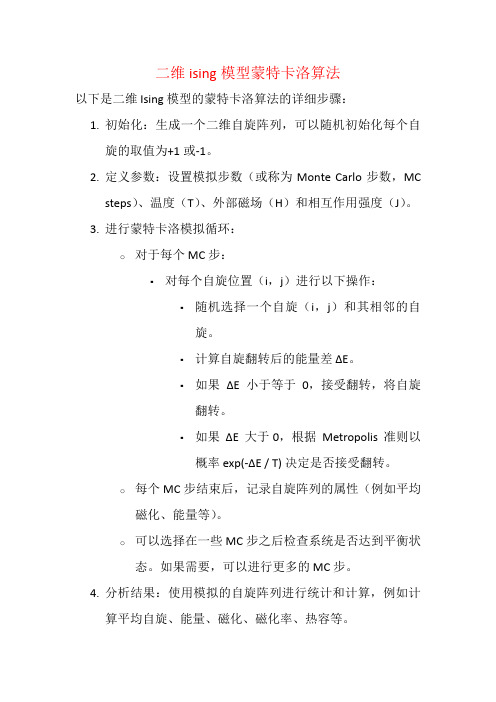
以下是二维 Ising 模型的蒙特卡洛算法的详细步骤:
1.初始化:生成一个二维自旋阵列,可以随机初始化每个自
旋的取值为+1或-1。
2.定义参数:设置模拟步数(或称为Monte Carlo 步数,MC
steps)、温度(T)、外部磁场(H)和相互作用强度(J)。
3.进行蒙特卡洛模拟循环:
o对于每个 MC 步:
▪对每个自旋位置(i,j)进行以下操作:
▪随机选择一个自旋(i,j)和其相邻的自
旋。
▪计算自旋翻转后的能量差ΔE。
▪如果ΔE 小于等于0,接受翻转,将自旋
翻转。
▪如果ΔE 大于0,根据Metropolis 准则以
概率 exp(-ΔE / T) 决定是否接受翻转。
o每个 MC 步结束后,记录自旋阵列的属性(例如平均磁化、能量等)。
o可以选择在一些 MC 步之后检查系统是否达到平衡状态。
如果需要,可以进行更多的 MC 步。
4.分析结果:使用模拟的自旋阵列进行统计和计算,例如计
算平均自旋、能量、磁化、磁化率、热容等。
这是基本的二维Ising 模型的蒙特卡洛算法步骤。
在实施算法时,还可以根据需要考虑边界条件(如周期性边界条件)、优化算法以提高效率等其他因素。
dft计算 建模六方晶系转化为直角

DFT计算是指密度泛函理论计算,它是一种计算化学方法,用于研究分子和固体的结构、性质和反应。
建模六方晶系转化为直角晶系是固体结构转变的一种典型情况,下面我们将通过DFT计算来探讨这一过程。
1.背景介绍在固体物理和材料科学中,晶体结构的转变是一个重要的研究课题。
其中,六方晶系和直角晶系是两种常见的晶体结构类型,它们之间的转变过程具有一定的复杂性和重要性。
采用DFT计算来研究六方晶系转化为直角晶系的过程,对于深入理解固体相变和晶体结构的转变机制具有重要意义。
2. DFT计算原理DFT计算是一种基于量子力学的计算方法,它利用密度泛函理论和库仑相互作用来描述原子和分子的电子结构和能量。
通过求解Kohn-Sham方程,可以得到系统的基态能量和波函数,从而进一步研究各种物理和化学性质。
在研究固体结构转变时,DFT可模拟晶格参数、晶胞体积、晶体对称性等物理量的变化,为理论预测提供重要的依据。
3. 六方晶系和直角晶系的简要介绍六方晶系是一种盒状结构,其晶胞参数a=b≠c,α=β=90°,γ=120°。
而直角晶系是一种长方体结构,其晶胞参数a≠b≠c,α=β=γ=90°。
两者在结构上具有明显的差异,因此六方晶系转化为直角晶系需要克服一定的能垒,因此具有一定的难度。
4. 计算步骤我们需要准备计算所需的原始数据,包括六方晶系的初始结构和晶格参数,以及计算所需的软件和计算资源。
我们将利用DFT方法对初始结构进行材料建模和能带计算,并计算出初始结构的能量和电子结构。
我们将通过改变晶格参数和/或应力的方式,模拟六方晶系向直角晶系转变的过程,并计算各个过渡态的能量和结构参数。
我们将分析计算结果,得出六方晶系转化为直角晶系的能垒和转变路径。
5. 计算结果与讨论通过DFT计算,我们得到了六方晶系转化为直角晶系的能垒和转变路径。
我们发现,在一定的外界条件下,六方晶系可以通过调控应力或温度等方式转变为直角晶系,其转变路径和能垒均与材料的晶体结构和物理性质密切相关。
HARDWARE-ACCELERATED
Revolutionary Visual Computing SolutionsHardware-Accelerated Pixel Read-Back Ultra-fast pixel read-back performance delivers massive host throughput, more than 10x the performance of previous generations of graphics systems.GPU ComputingNVIDIA CUDA provides a C languageenvironment and tool suite that unleashes new capabilities to solve complex, visualization challenges such as real-time ray tracing and interactive volume rendering.1NVIDIA PureVideo TechnologyNVIDIA PureVideo ™ technology is the combination of high-definition video processors and software that deliversunprecedented picture clarity, smooth video, accurate color, and precise image scaling for SD and HD video content. Featuresinclude, high-quality scaling, spatial temporal de-interlacing, inverse telecine, and high quality HD video playback from DVD.Features and BenefitsFull 128-Bit Precision Graphics Pipeline Enables mathematical computations to maintain high accuracy, resulting in unmatched visual quality.High-Quality Full-Scene Antialiasing (FSAA)Up to 32x FSAA dramatically reduces visual aliasing artifacts or “jaggies” at resolutions up to 2560 x 1600, resulting in highly realistic scenes. New rotated-grid FSAA algorithm (RG FSAA) delivers unprecedented quality and performance.High Precision, High Dynamic Range Imaging (HDR)Sets new standards for image clarity and quality through floating point capabilities in shading, filtering, texturing, and blending. Enables unprecedented quality of rendered images for visual effects processing.NVIDIA Unified ArchitectureIndustry’s first unified architecture designed to dynamically allocate geometry, shading, pixel, and compute processing power to deliver optimized GPU performance.1Dual Dual-Link Digital Display Connectors Dual dual-link TMDS transmitters support ultra-high-resolution panels (up to 2560 x 1600 @ 60Hz on each panel) − which result in amazing image quality producing detailed photorealistic images.3Essential for Microsoft Windows Vista Offering an enriched 3D user interface,increased application performance, and the highest image quality, NVIDIA Quadro graphics boards and NVIDIA ® OpenGL ICD drivers are optimized for 32- and 64-bit architectures to enable the best Windows ® Vista ™ experience.Technical SpecificationsNVIDIA QUADRO WORKSTATION GPU > 12-bit subpixel precision > Up to 128 textures per pass > Eight (8) multiple render targets > Fast 3D texture support > Jumbo (8K) texture support> Hardware-accelerated antialiased points and lines> Hardware OpenGL overlay planes> Hardware-accelerated two-sided lighting > Hardware-accelerated clipping planes > Third-generation occlusion culling > OpenGL quad-buffered stereo (3-pin sync connector)> Hardware-accelerated pixel read-back NEXT-GENERATION SHADING ARCHITECTURE> Full Shader Model 4.0 (OpenGL and DirectX 10) o Vertex Shader 4.0 o Geometry Shader 4.0 o Pixel Shader 4.0> Unlimited Shader Lengths> FP32 texture filtering and blending > Non-power-of-two texture supportNVIDIA CUDA Software Development Tools > C language compiler, profiler and emulation mode for debugging> Standard numerical libraries for FFT (Fast Fourier Transform) and BLAS (Basic Linear Algegra Subroutines)HIGH-LEVEL SHADER LANGUAGES > Optimized compilers for Cg, OpenGLSL, and Microsoft HLSL > OpenGL 2.1 and DirectX 10 support > Open source compilerHIGH-RESOLUTION ANTIALIASING > Up to 32x full-scene antialiasing (FSAA), up to 2560 x 1600> Rotated-grid FSAA significantly increases color accuracy and visual quality for edges, while maintaining performance UNIFIED DRIVER ARCHITECTURE > Single driver supports all products SUPPORTED PLATFORMS> Microsoft Windows ® Vista, XP, 2000 > Linux—Full OpenGL implementation, complete with NVIDIA and ARBextensions (complete XFree 86 drivers)> AMD64, Intel EM64TPROFESSIONAL CERTIFICATIONS Computer-Aided Design (CAD) /Computer-Aided Manufacturing (CAM) /Computer-Aided Engineering (CAE) Applications > AutoCAD > CATIA > DeltaGen > Inventor > PDMS > PLM> Pro / ENGINEER > Revit> Solid Edge > SolidWorks> and many more…Digital Content Creation (DCC) and Broadcast > 3ds Max > After Effects > Houdini > Illustrator > Lightwave > Maya> Premiere Pro > Softimage | XSI > and many more…Energy> Landmark> Paradigm GEO > Schlumberger Medical/Life Sciences > Accelyris > Tripos> Vital Images1 Available on NVIDIA Quadro FX 5600, 4700 X2, 3700, 1700, 570, 370, 3600M, 1600M, 570M, and 360M.2 Available on NVIDIA Quadro FX 5600, 5500, 4700 X2, 4600, 4500, 3700, 3500, and 3450.3 Available on NVIDIA Quadro FX 5600, 5500, 4700 X2, 4600, 3700, 3500, 1700, and 1500.For more information about NVIDIA Quadro, visit © 2007 NVIDIA Corporation. All rights reserved. NVIDIA, the NVIDIA logo, NVIDIA Quadro, Cuda, and SLI are trademarks and/or registered trademarks of NVIDIA Corporation.All company and product names are trademarks or registered trademarks of the respective owners with which they are associated. Features, pricing, availability, and specifications are all subject to change without notice. Images courtesy of Right Hemisphere, Landmark, UVPHACTORY, NVIDIA Corporation, and Vital Images,The industry’s leading workstation applications leverage these solutions to enable hardware-accelerated features not found in any other professional graphics solution.The Quadro professional products include a set of industry specialtysolutions that have been architected to enable advanced imaging visualization and broadcast applications - from multi-system scalability andsynchronization to uncompressed 12-bit HD-SDI video output.The NVIDIA Quadro ® family of professional solutionstakes the leading professional applications to a new level of interactivity by enabling unprecedented capabilities.Images courtesy of Right Hemisphere, Landmark, a brand of the Halliburton Drilling, Evaluation and Digital Solutions, UVPHACTORY, and Vital Images, Volvo Image Copyright © 2006 MFX / Percival Productions. www.mfx.se.NVIDIA Quadro Family | Sep 2007Ground-breaking Unified Architecture Delivers Unprecedented Performance The latest NVIDIA Quadro architecture takes application performance tonew levels by featuring the industry’sfirst unified architecture1. Designed to dynamically allocate geometry, shading, pixel, and compute processing power, the latest NVIDIA Quadro graphics boards deliver optimized Graphics Processing Unit (GPU) performance. The GPU pipeline efficiency is further multipliedby fast 3D and large texture transfers, NVIDIA’s crossbar memory architecture, enabling occlusion culling, lossless depth Z-buffer, and color compression. These elements combine to achieveunprecedented 3D performance: blazinggeometry performance, lightening-fastline performance and massive fill ratespowered by a dynamically configurablearray of thread processors. With ultra-fast pixel read-back performance,massive host throughput gains can beachieved for professional applications.However, the true measure of power isapplication performance and the newNVIDIA Quadro architecture doubles theperformance of the previous generation.Advanced ProgrammabilityEmpowers a New Classof ApplicationsThe latest NVIDIA Quadro FX graphicssolutions are the reference standard forShader Model 4.0 and next generationoperating systems enabling breakthroughultra-realistic, real-time visualizationapplications. Styling and productionrendering are integral functions of thedesign workflow and NVIDIA QuadroFX provides professionals the toolsto shorten the production processand enable faster time to market.The major CAD and DCC applicationvendors can take full advantage of theprogrammable NVIDIA Quadro architectureby enabling sophisticated shaders tosimulate a virtually unlimited range ofphysical characteristics, such as lightingeffects (dispersion, reflection, refraction,BRDF models) and even physical surfaceproperties (casting effects, porosity,molded surfaces). Real-time shaders allowaccurately matching visual images.All images have a smoother, moreappealing variation in color density, whichincreases visual realism and generatesphotorealistic rendered images.Certified for the HighestQuality Experience withthe Most DemandingWorkstation ApplicationsThe performance and power of theNVIDIA Quadro architecture arebuilt on a solid foundation of qualityengineering. This engineering excellenceis exemplified by the NVIDIA UnifiedDriver Architecture (UDA), which iscertified for quality by the entire spectrumof CAD and DCC applications.these effects to be combined and modifiedinteractively, something that is impossiblewith simple 2D static texture maps.Full 128-bit Floating PointPrecision Delivers the Industry’sHighest Workstation QualitySophisticated real-time effects typicallyinvolve multiple mathematical operations thatdemand high precision to maintain imagequality. The NVIDIA Quadro architecturefeatures true 128-bit IEEE floating pointprecision (32-bit fp per component),resulting in the highest level of accuracyand the ultimate in visual quality.The NVIDIA Quadro family delivers true16-bit and 32-bit floating point formats forThe Definition of Performance. The Standard for Quality.uncompromisedprofessional graphics to goThe NVIDIA Quadro FX professional solutions for mobile workstations deliver the fastest application performanceand the highest quality graphics. The NVIDIA Quadro FX mobile solutions enable the leading CAD, DCC, and visualization applications to solve the most complex professional visual computing challenges in a mobile form factor.integrated graphics to video solutionThe NVIDIA Quadro SDI solutions are ideal foron-air broadcast professionals across manyapplications, including virtual-set, sports, andweather news systems. The NVIDIA Quadro SDIsolution is the industry’s only fully integratedgraphics to video out product, and will compositelive video footage onto virtual backgrounds andsend the result to live video for TV broadcast. Thesolution also allows film production and post-production professionals to preview the results of3D compositing, editing, and color grading in realtime on HD broadcast monitors.c programming environmentfor the gpuThe NVIDIA CUDA™software development kitprovides a C language environment and toolssuite that unleashes new capabilities to solvecomplex, visualization challenges such asreal-time ray tracing and interactive volumerendering.1revolutionizingadvanced visualizationThe NVIDIA Quadro G-Sync deliversframe and genlock functionality tounprecedented levels of industrialrealism, visualization, and collaborativecapabilities. The NVIDIA Quadro G-Sync IIoption can be combined with the QuadroFX 5600 or 4600, and G-Sync I can becombined with the FX 5500 to provideadvanced multi-system visualizationand external signal synchronization.a quantum leap in visual computingThe NVIDIA Quadro Plex is a dedicatedvisual computing system (VCS) enablingbreakthrough levels of capability andproductivity for professionals ranging frommanufacturing designers and stylists toearth scientists to digital content creators.NVIDIA Quadro Plex provides the flexibility tobe deployed with any certified PCI Express®x16 platform. NVIDIA Quadro Plex achievesunmatched compute density, can bedeployed in a wide range of environments,and scales to meet the most demandingprofessional applications requirements.HP Mobile Workstation courtesy HP - image on screen courtesy ProE2000. Racetrack image © Sam Sharpe / The Sharpe Image / Corbis. Inside right page: Geographic imagery courtesy Landmark, a brand of the Halliburton Drilling, Evaluation and Digital Solutions. Video Wall image courtesy ORNL.scalable graphics performance NVIDIA Quadro graphics solutions feature NVIDIA® SLI™ multi-GPU technology2.A revolutionary platform innovation,SLI technology enables professional users to dynamically scale graphics performance, enhance image quality, and expand display real estate by combining multiple NVIDIA Quadro graphics solutions in a single system.Available NVIDIA Quadro Solutions Ultra-High-EndNVIDIA Quadro FX 5600 NVIDIA Quadro FX 5500 NVIDIA Quadro FX 4700 X2 High-EndNVIDIA Quadro FX 4600 NVIDIA Quadro FX 3700 NVIDIA Quadro FX 3500Mid-RangeNVIDIA Quadro FX 3450 NVIDIA Quadro FX 1700 NVIDIA Quadro FX 1500 Entry-LevelNVIDIA Quadro FX 570 NVIDIA Quadro FX 560 NVIDIA Quadro FX 550 NVIDIA Quadro FX 370 SpecialtyNVIDIA Quadro Plex VCS NVIDIA Quadro SDINVIDIA Quadro G-Sync MobileNVIDIA Quadro FX 3600M NVIDIA Quadro FX 1600M NVIDIA Quadro FX 570M NVIDIA Quadro FX 360M。
基于最大熵和粒子群优化的红外图像分割英文
第30卷 第5期2007年10月电子器件Ch inese Jou r nal Of Elect ro n DevicesVol.30 No.5Oct.2007Maximum Fuzzy Entr opy and Par t icle Sw ar m Optimizat ion (PSO)B a sed Inf rar ed Image Segmenta tion 3Z H A N G Wei 2w ei 1,TA N G Yi n g 2ga n21.Insti t ute of In f ormati on Engi neeri ng ,Hebei I nst i t ut e of Technolo gy ,Tan gs han Hebei 063000,China ;2.I nst i t ut e of Elect rical En gi neeri ng ,Yansh an Uni versit y ,Qi ng huang dao Hebei 066004,ChinaAbstract :Maxi mum f uzzy ent ropy has been proven to be an efficient met hod for i mage segmentation.The key problem associate d wit h t hi s met hod is to find t he opt imal paramet er com bi nation of membe rship f unc 2t ion so t hat an i mage can be t ransfor med into f uzzy domai n wi t h maxi mum fuzzy ent rop y.However ,i t is computationall y i nt ensi ve or even impossibl e to fi nd t he optimal parameter combi nation of mem bership function direct l y.A new optimizat ion al gorit hm ,namely ,P SO al gorit hm i s used to search opt imal para me 2t er com bination.Each parti cle represent s a po ssible paramet er com bi nat ion.A swa rm of particles are ini 2t ialized and fly t hrough solution space for tar get ing t he opti mal solution.The p roposed met hod i s used t o segment i nf rared i ma ge and ideal segmentat ion result s ca n be obt ai ned wit h less computat ion cost.K ey w or ds :inf rared image ;i mage se gmentation ;f uzzy ent ropy ;part icle swarm opt imizat ion (PSO)EEACC :6140C基于最大熵和粒子群优化的红外图像分割3张薇薇1,唐英干21.河北理工大学信息学院,河北唐山063000;2.燕山大学电气工程学院,河北秦皇岛066004收稿日期6228基金项目国家自然科学基金中杰出青年学者资助项目(65533);河北省教育厅基金资助项目()作者简介张薇薇(2),女,硕士,河北理工大学教师,主要研究方向为图像处理和模式识别,zjz @63摘 要:最大模糊熵是一种有效的图像分割方法,该方法的一个关键问题是确定模糊隶属度函数的最优参数组合,从而使得图像变换到模糊域后的模糊熵最大.但是直接采用穷举法来寻找最优参数组合的计算量是很大的,甚至是不可能的.因此,提出了采用一种新的优化方法,即粒子群算法来寻找最优参数组合.在参数搜索空间中,随机初始化一群粒子,通过粒子之间的相互协作来寻找最优解.所提出的方法用于分割红外图像的结果表明,花费很小的计算代价就可以获得理想的分割结果.关键词:红外图像;图像分割;模糊熵;粒子群中图分类号:TP391.41 文献标识码:A 文章编号:100529490(2007)0521736205 Infrared image segment at io n ,which ext ract s object s f ro m background ,plays an import ant role i n auto mat ic t arget recognit ion (AR T)and i nf rared guidance techni que.Thresholdi ng i s a most used met hod to segment inf rared i mage for it s si mplici t y and l ess comput ation cost.However ,i nf ra red i m 2age po ssesse s low cont rast bet ween object andbackground and t he edge of object is am biguous ,cla ssical t hreshol d select ion met hod ,such a s Ot 2su [1]a nd Kapur [2]approach ,can usually not obtain an i deal segment ation resul t s.Fuzzy set t heory i s a powerf ul mat hematic tool ha ndli ng a mbiguit y or uncert ai nt y and has bee n ap 2plied to image segment ation successf ully.Fuzzy c 2part ition is a popul ar f uzzy segmentat ion met hod.:200092:020*******:1977w w 1.co m.Cheng,et al[3].proposed to use f uzzy c2parti tionand maxi mum ent ropy p ri nciple to select t hreshol d automatical ly.Cheng,et al[4],defined a new f uzzy ent rop y and used it t o image segment ation and e n2 hance.Zhao,et al[5]proposed an ot her e nt ropy function using f uzzy c2partit ion and proba bili t y partit ion.Tao[6]proposed a n i mproved ve rsion of Zhao’s met hod and used i t to select t hree2level t hreshol d.A lt hough t he f uzzy c2pa rtition app roach for im age t hre sholdi ng result s i n much bet t er se g2 mentat ion t han many exi sting met hods,t he com2 putat io n burden i s very large because t he size of searc h space increases when t he number of param2 ete rs needed to det ermi ne t he m em ber ship f unc2 t ion increa ses.For example,if S2f unction and Z2 function wi t h t hree paramet ers(i.e.a,b,c)i s se2 lect ed to const ruct f uzzy c2partition,t he searc h space i s L(L-1)(L-2)/6for an i mage having L gray level s.I f L equal s256,t hen t he sea rch space will be2763520.It i s impo ssible to sea rch opti mal parameter com binat ion direct ly.Ma ny resea rcher s seek help to genetic al gorit hm(GA)[4,6]and simu2 lat ed anneali ng(SA)[3,5]to solve t hi s problem.Al2 t hough GA a nd SA can usually obt ai n opt imal so2 l ution,t hey are equipped wit h some drawbacks such a s ea rl y mat uration of G A and slow conver2 gence of SA.PSO i s an evolutionary opt imization t ec hni que developed by K ennedy a nd Eberhart i n1995[7]in2 spired by t he beha vior of bi rd flocking a nd fish schooli ng.Li ke G A,PSO i s a pop ulation2ba sed al2 gori t hm,each i ndi vi dual o r candidat e solution i s call ed a“part icle”.PSO i s effecti ve i n nonli near opti mization problem s and easy to i mple me nt.PSO and it s i mprovement versions have been applied i n ma ny area s such as reacti ve power opt imization[8], polygo nal app roxi mat ion[9]and combi natori al opt i2 mizat ion[10]et c.In t hi s paper,P SO i s used to find t he opti mal parameter combi nation based on ma xi2 m um f uzzy ent ropy p ri ncipl e.Each part icle repre2 se nt s a possi ble parameter combination.Inf rared 1 Threshold Select ion Using Fuzzy Entr opy Pr inciple L et I be a n image of size M×N and I(x,y)be t he gray l evel of pi xel(x,y),where I(x,y)∈{0, 1,2,…,l-1}.The hi stogra m of image I i s rep re2sent ed by H={p0,p1,…,p l-1}where p k=n kM×N and n k i s t he num ber of pi xel wi t h gray l evel k.As2 sume t hat i mage I i s sepa rat ed i nto object E o a nd background E b by t hreshold T,t hen it s probabilit y i s p o=p(E o)and p b=p(E b).For each gray l evel k(k=0,1,2,…,l-1),t he proba bi li t y belongi ng to object a nd background arep k0=p k×p o|k a nd p kb=p k×p b|k(1) respectivel y,where p o|k and p b|k are t he co nditional p roba bili t y of gray l evel k belongi ng to object a nd background.In t hi s paper,l et t he co nditional p roba bili t y of gray l evel k belongi ng to object a nd background equal to fuzzy member ship of gray lev2 el k t o o bj ect and background,i.e.p o|k=μo(k),p b|k=μb(k)(2)whereμo(k)andμb(k)a re t he f uzzy member2 ship of gray level k to object and background.It can get from Equ.(1)a nd Equ.(2):p o=p(E o)=∑l-1k=0p ko=∑l-1k=0p k×p o|k(3) p b=p(E b)=∑l-1k=0p kb=∑l-1k=0p k×p b|k(4) We choose t he S2f unction and Z2function de2 fined in Equ.(5)a nd Equ.(6)a s t he mem bership f unction of object a nd background respectively,μo(k)=S(k;a,b,c)=0 kΦa(k-a)2(c-a)(b-a) a<kΦb1-(k-c)2(c-a)(b-a) b<kΦc1 k>c(5)μb(k)=Z(k;a,b,c)=1-S(k;a,b,c)(6) where0<aΦbΦc.He nce,t he f uzzy e nt ropy of obj ect and background i s=∑=×μ()×μ()()7371第5期张薇薇,唐英干:基于最大熵和粒子群优化的红外图像分割image is segmented using the proposed method andideal results can be obtained with le ss comp uta tion cost.H o-l-1k0p k o kp oln p k o kp o7 andH b =-∑l-1k =0p k ×μb (k)p bln p k ×μb (k )p b(8)The t ot al f uzzy ent rop y f unction is gi ve n a s followingH (a ,b,c )=H o +H b(9)The t otal fuzzy e nt ropy varies along wit h t hree varia bles a ,b ,c .We can fi nd an opti mal com binat ion of (a ,b ,c )so t hat t he t ot al f uzzy en 2t ropy H (a ,b ,c )ha s maxim um val ue.Then ,t he most approp riat e t hreshold T can be comput ed asμo (T )=μb (T )=0.5(10)However ,find t he opt imal com binat ion of (a ,b ,c)i s not a n ea sy wor k as t he reaso n ment io ned previously.In t his paper ,a new opti mization algo 2rit hm ,namel y t he pa rticle swarm opti miza tion (PSO )i s used to find t he opti mal com bi nat ion of (a ,b ,c ).2 PSO A lgor ithmThe basic P SO model consist s of a swar m of particles movi ng in a d 2di mensional search space w he re a ce rtain qualit y measure ,t he fit ness ,can be calculated.Each pa rticl e ha s a po si tio n repre 2sent ed by a vector x i =(x i1,x i2,…,x id )and a velocit y rep re sented by vector v i =(v i1,v i2,…,v id ),where i is t he i nde x of part icle.W hile searc hing opti mal solution in search space ,each particle re mem ber s t wo vari able s:one i s t he best position fo und by it s ow n so far ,denoted by p i a nd anot her i s t he best posit ion among all pa rticle s in t he swar m ,denoted by p g .A s ti me pa sse s ,each particle up date s it s position and velocit y to a new value accor ding t o form ula Equ.(11)a nd Equ.(12)v i (t +1)=w 3v i (t)+c 13r 13(p i -x i (t))+c 23r 23(p g -x i (t ))(11)x i (t +1)=x i (t )+v i (t +1),i =1,2,…,n(12)Where w is t he ine rtia weight ,c 1and c 2are t he lea rning factor s ,ge nerall y ,c 1=c 2=2,r 1,and r 2are two ra ndom number wi t hin t he i nt erval of (0,1),t i s t he number of i teration.G enerally ,t he value of each component s in v i can be clamped [x ,x ]x 2f T f Equ.(12).Thi s process i s repeated until a user 2de 2fined stoppi ng cri terion i s reac hed.In t hi s paper ,PSO i s used fi nd t he opt imal pa 2rameter com bination.Each part icle represent s a possi ble pa ramet er combination.The tot al fuzzy ent ropy i s use d as t he fit ness of each particle.The segment ation procedure usi ng f uzzy ent ropy a nd PSO can be depict ed as followi ng :(1)Ra ndomly generate n part icle s of 32di men 2sion.Each particle is a ssigned a randomized veloci 2t y and posit io n.Set t he ma xi mum it erat io ns N a nd let t =0.(2)Calc ulate t he fi t ness of each part icle usi ng Equ.(9).(3)Updat e t he per sonal be st of eac h parti cles accordi ng to it s curre nt fi t ness and global best a 2mo ng all particles accordi ng t he fit ness of t he swarm s.(4)Cha nge t he velocit y of each particl e usi ng Equ.(11)(5)Move each parti cle to it s new position u 2sing Equ.(12)(6)Let t =t +1and go to St ep 2.Repeat untilt =N(7)Out put t he best position of t he swarm.Calcul at e t he best t hreshold using Equ.(10).3 Exper imental ResultsTo eval uat e t he perform ance of t he proposed met ho d ,experi ment s have been car ried on two i n 2f rared ima ges usi ng MA TL AB 6.5on Pentium 2IV 2.66GHz .The t est im ages are factory a nd t ank whose size i s 185×255and 176×126respec 2tively.Several met hods ,i. e.,Ot su ,Kap ur ,f uzzy e nt ropy usi ng GA i n Ref.[6]are used to seg 2me nt t hese images as well as t he p ropo se d met h 2od.The segm ent ation re sult s are show n i n Fi g.1and Fig.2and t hreshol ds o bt ai ned by t hese met h 2ods a re li st ed i n Table 1.It can be seen from t he result s t hat t he se gm ent ation result s obt ai ned by f uzzy ent ropy met hod are bet t er t han Ot su and Kapur met hod because m uch fal se object ’s i nfor 2x y O K 8371电 子 器 件第30卷to t he range -v ma v ma to control e cessive roa ming o pa rticle s outside the search space.he particle lie s toward to a new position according tomatio n e ist in the results obtained b tsu and apur method.(a )original ima ge (b )Ot su method (c )K apure method(d)f u zzy en tropy method using G A in Re f.[6] (e)f u zzy entropy meth od using PSO (f)total entropy at each iterati on using G A and PSOFig.1 Segmentation results of image f actor y To demonst rat e t he good performance of PSO ,G A is al so used to find t he opti mal paramet er co mbina 2t ion.The paramet ers of GA are set a s i n Ref.[6].Iteration number of G A and PSO are bot h 100.The best parameter combi nation ,t he best tot al fuzzy ent rop y and computation t ime obt ai ned by GA a nd PSO are shown i n Table 2.The cha nge of t otal fuzzy ent ropy at each it era tion using G A a nd PSO are shown in Fi g.1(f)and Fi g.2(f).From Fi g.1(d)-(e)and Fig.2(d)-(e),we can see t hat t he segmentat ion re 2sult s a re compa rat ive usi ng G A and PSO and t he best tot al f uzzy ent ropy is almost t he same.However ,t he computation ti me usi ng PSO i s m uc h less t han usi ng GA.The comput ation t ime using PSO i s a bo ut 1/4of G A.So ,i t i s much fa ster usi ng PSO t han G A.In t hi s paper ,we do not compare t he comput ation ti me u 2si ng PSO and e xha ust searching met hod because i t i s a very t ime 2co nsuming work usi ng exhaust searchi ng met hod to fi nd t he opti mal pa ra met er com binat io n.However ,we can e sti mat e t he comput ation ti me roughl y.In our experi ment ,about 0.05second i s used t o compute t he tot al f uzzy ent ropy each ti me.If ex 2haust searching is used ,about 138162seco nds ,i.e.about 38hour s should be used a nd it cannot be t oler 2ant i n real ti me syst em.(a)original ima ge (b)Ot su method (c)K apure method()f zzy y G R f [6] ()f zzy y SO (f)y G SOF S f 9371第5期张薇薇,唐英干:基于最大熵和粒子群优化的红外图像分割d u en trop method using A in e .e u entrop meth od using P total entrop at each iterati on using A and P ig.2e gmentation results o image tankT a b.1 Thr eshold obta ined by Otsu,K a pur,GA an d PSOImageMethodOtsu K apur GA PSOfactory64109141142 tank107140180180T a b.2 Computa tion time,total thr eshold and par ameter combina tion(a,b,c)of G A a nd PSOtermf actor y tankG A PSO GA PSOtime(s)8.859 2.1579.14 2.25 total entropy9.35799.358210.45310.462 (a,b,c)(51,173,186)(51,179,179)(0,255,255)(0,255,255)4 ConclusionIn co ncl usion,a new segment ation scheme i s proposed for i nf rared ima ge.The i mage t o be se g2 mented i s t ransformed i nto f uzzy domain using S2 function and Z2f unction wit h t hree parameter s. The best t hre shol d is obt ai ned based on maxi mum fuzzy ent ropy pri nciple.PSO algorit hm i s use to find t he best parameter co mbination of S2f unction and Z2f unction.It i s show n t hat,P SO al gorit hm can obtain t he best parameter com bination wit h less comput ation cost t ha n many existi ng met hod such a s e xha ust searching and G A.It p rovides a good qualificat ion for real ti me syst em.R eferences:[1] Ot su N.A Threshol d Select ion Met ho d f ro m Gray2L evel His2t ogram[J].IEEE Tran s.on Syst em s,Man and Cyberneti c, 1979,9(1):62266.[2] K apur J N,Sahoo P K,W o ng A K C.A New Met hod forGray2Level Pict ure Th res hol di ng using t he ent rop y of t he hi s2 t ogram[J].C o m p ut er Vi sion,G raphics and Im age Pro cess2 in g,1985,29(3):2732285.[3] Chen g H D,Chen J R,Li J G.Th res hol d Sel ect ion Based onFuzzy c2Parti tio n Ent ropy Approach[J].Patt ern Recognit ion, 1998,31(7):8572870.[4] Chen g H D,Hung Y H and Sun Y.A Novel Fuzzy Ent ropyApp roach t o Im age Enhancem ent and Threshol ding[J].Signal Proces s i ng,1999,75(3):2772301.[5] Zhao M S,Fu A M N,Yan H.A Tech ni que of Three LevelTh res hol di ng Based o n Probabi lit y Partit ion and Fuzzy32Part i2 t ion[J].I EEE Tran s.Fuzzy Syst em s,2001,9(3):4692479.[6] Tao W B,Tian J W and Li u J.Image Segment atio n by T hree2Level Thresholdin g Based on Maxi mum Fuzzy Ent ropy and Genet ic Algorit h m[J].Patt ern Recognit ion L et t er s,2003,24(16):306923078.[7] Ken nedy J,Ebert hart R C.Par ticl e Swarm Opt i m izat ion[C]//Proc.IEEE Int er nat.Co nf.On Neural Network s,Piscat2 away,NJ,USA:194221948.[8] Ji ang C W,Bo m pard W.A Hybrid Met hod fo Chaot ic Part icl eSwarm Op ti m izat ion and Li near Interior fo r Reacti ve Power Opt imizat ion[J].Mat hem ati cs and C o mput ers i n Sim ul at ion, 2005,68(1):57265.[9] Yin P Y,A Discret e Part icl e Swarm Al go ri t hm for Opt imalPolygonal App ro xi mation of Di gi t al Curves[J].Jo urnal of Vi s2 ual C o mmu nicat ion and Image Rep resent ation,2004,15(2): 2412260.[10] Sal man,Ahmad I and Madani S A.Parti cle Swarm Opt imiza2t ion fo r Task Asignment Poblem[J].Mi croprocessor s andMicrosys tems,2002,26(8):3632371.0471电 子 器 件第30卷。
蒙特卡罗方法数值模拟二维原子光刻

文 章 编 号 : 2 33 4 2 1 ) 81 7 ・6 0 5 —7X(0 2 0 —2o0
D :0 36 /. s .2 33 4 . 0 2 0 . 2 OI1 .9 9ji n 0 5 —7x 2 1 .8 0 6 s
蒙 特 卡 罗 方 法 数 值 模 拟 二 维 原 子 光 刻
张萍萍 , 马 艳 , 同保 李
第 4 第 8期 0卷 21 0 2年 8月
同 济 大 学 学 报 ( 然 科 学 版) 自
J l N I O O G I Nv R I Y N O 『 A . FT N J U I E ST ( 枷 IA , c E C ) R I I S I N E {
VOI4 . 0 No. 8 Au . 2 1 g 02
n n s l e g r n f r sa d r . F c sn n e o iin a o c e ln t ta se t n a d a h o u i g a d d p st o c a a trs i s o q a r t o t l a t e o me b t h r c e itc f u d a i c p i l ti f r d y wo a c c
( 济 大学 物 理 系 , 海 2 0 9 ) 同 上 0 0 2
摘 要 :间距 为半 波 长 的 纳Байду номын сангаас 点制 作 可 以进 一 步 推 动 纳米 计 量
各 种纳 米 级 科 学测 量 仪 器 , 别 是作 为 纳米 科 特
的发展. 基于经典粒 子光学 模型 , 采用 蒙特 卡 罗思想 提供 初 技 主要 测 量 和 操 作 工 具 的原 子 力 显 微 镜 ( M) AF 和 始 条 件 , 值 分 析 了 偏 振 方 向平 行 于 光 场 平 面 、 交 激 光 驻 扫描 电子 显 微 镜 ( E ) , 数 正 S M 等 由于 受 仪 器 工 作 原 理 、
集成电路的集成度 英语

集成电路的集成度英语The Integration of Integrated CircuitsThe world of electronics has undergone a remarkable transformation over the past few decades, and at the heart of this revolution lies the integrated circuit. Integrated circuits, or ICs, have become the backbone of modern electronic devices, enabling the developmentof increasingly sophisticated and compact technologies. One of the key aspects of integrated circuits that has driven this innovation is the concept of integration density, which refers to the number of transistors and other electronic components that can be packed onto a single integrated circuit.The history of integrated circuits can be traced back to the 1950s, when the first integrated circuit was developed by Jack Kilby at Texas Instruments. Kilby's invention was a significant breakthrough, as it allowed multiple electronic components to be integrated onto a single semiconductor chip, rather than having to connect them individually. This not only reduced the size and complexity of electronic devices but also improved their performance and reliability.As the technology continued to evolve, the integration density ofintegrated circuits began to increase exponentially. This phenomenon is often referred to as Moore's Law, named after Gordon Moore, the co-founder of Intel. Moore's Law states that the number of transistors on a microchip doubles approximately every two years, while the cost of computers is halved. This trend has held true for several decades, and it has driven the rapid advancement of integrated circuit technology.One of the key factors that has enabled the increasing integration density of integrated circuits is the development of semiconductor fabrication processes. These processes, which involve the precise manipulation of materials at the atomic level, have become increasingly sophisticated and precise, allowing for the creation of ever-smaller and more complex integrated circuits.The most common semiconductor fabrication process used in the production of integrated circuits is known as complementary metal-oxide-semiconductor (CMOS) technology. CMOS technology relies on the use of two types of transistors, known as n-type and p-type, which are arranged in a complementary fashion to create logic gates and other electronic components. As the size of these transistors has decreased, the integration density of integrated circuits has correspondingly increased.Another important factor in the increasing integration density ofintegrated circuits is the development of advanced lithography techniques. Lithography is the process of transferring a pattern onto a semiconductor wafer, and it is a critical step in the fabrication of integrated circuits. As the size of transistors and other components has decreased, the resolution of the lithography process has had to improve accordingly, allowing for the creation of ever-smaller and more complex integrated circuits.The impact of increasing integration density on the electronics industry has been profound. As integrated circuits have become more compact and powerful, it has enabled the development of a wide range of electronic devices, from smartphones and laptops to medical equipment and industrial control systems. The ability to pack more functionality into a smaller physical space has also led to significant improvements in energy efficiency, as well as reductions in the cost and weight of electronic devices.However, the continued scaling of integrated circuits is not without its challenges. As transistors and other components become smaller, they become more susceptible to various physical and electrical effects that can degrade their performance and reliability. Additionally, the cost of developing and manufacturing the most advanced integrated circuits has become increasingly prohibitive, requiring significant investments in research and development, as well as in specialized fabrication facilities.Despite these challenges, the drive to increase the integration density of integrated circuits shows no signs of slowing down. Researchers and engineers are constantly exploring new materials, device structures, and fabrication processes in an effort to push the boundaries of what is possible. The development of technologies such as three-dimensional transistors, quantum computing, and neuromorphic computing hold the promise of further advancing the capabilities of integrated circuits and enabling even more innovative and transformative applications.In conclusion, the integration density of integrated circuits has been a key driver of the electronics revolution, enabling the development of increasingly sophisticated and compact electronic devices. The continuous scaling of integrated circuits, as predicted by Moore's Law, has been made possible through advancements in semiconductor fabrication processes and lithography techniques. While there are challenges to overcome, the ongoing pursuit of higher integration density promises to continue shaping the future of electronics and technology.。
高一科学探索英语阅读理解25题

高一科学探索英语阅读理解25题1<背景文章>The Big Bang Theory is one of the most important scientific theories in modern cosmology. It attempts to explain the origin and evolution of the universe. According to the Big Bang theory, the universe began as an extremely hot and dense singularity. Then, a tremendous explosion occurred, releasing an enormous amount of energy and matter. This event marked the beginning of time and space.In the early moments after the Big Bang, the universe was filled with a hot, dense plasma of subatomic particles. As the universe expanded and cooled, these particles began to combine and form atoms. The first atoms to form were hydrogen and helium. Over time, gravity caused these atoms to clump together to form stars and galaxies.The discovery of the cosmic microwave background radiation in 1964 provided strong evidence for the Big Bang theory. This radiation is thought to be the residual heat from the Big Bang and is uniformly distributed throughout the universe.The Big Bang theory has had a profound impact on modern science. It has helped us understand the origin and evolution of the universe, as well as the formation of stars and galaxies. It has also led to the development ofnew technologies, such as telescopes and satellites, that have allowed us to study the universe in greater detail.1. According to the Big Bang theory, the universe began as ___.A. a cold and empty spaceB. an extremely hot and dense singularityC. a collection of stars and galaxiesD. a large cloud of gas and dust答案:B。
重要哲学术语英汉对照

重要哲学术语英汉对照——转载自《当代英美哲学概论》a priori瞐 posteriori distinction 先验-后验的区分abstract ideas 抽象理念abstract objects 抽象客体ad hominem argument 谬误论证alienation/estrangement 异化,疏离altruism 利他主义analysis 分析analytic瞫ynthetic distinction 分析-综合的区分aporia 困惑argument from design 来自设计的论证artificial intelligence (AI) 人工智能association of ideas 理念的联想autonomy 自律axioms 公理Categorical Imperative 绝对命令categories 范畴Category mistake 范畴错误causal theory of reference 指称的因果论causation 因果关系certainty 确定性chaos theory 混沌理论class 总纲、类clearness and distinctness 清楚与明晰cogito ergo sum 我思故我在concept 概念consciousness 意识consent 同意consequentialism 效果论conservative 保守的consistency 一致性,相容性constructivism 建构主义contents of consciousness 意识的内容contingent瞡ecessary distinction 偶然-必然的区分 continuum 连续体continuum hypothesis 连续性假说contradiction 矛盾(律)conventionalism 约定论counterfactual conditional 反事实的条件句criterion 准则,标准critique 批判,批评Dasein 此在,定在deconstruction 解构主义defeasible 可以废除的definite description 限定摹状词deontology 义务论dialectic 辩证法didactic 说教的dualism 二元论egoism 自我主义、利己主义eliminative materialism 消除性的唯物主义 empiricism 经验主义Enlightenment 启蒙运动(思想)entailment 蕴含essence 本质ethical intuition 伦理直观ethical naturalism 伦理的自然主义eudaimonia 幸福主义event 事件、事变evolutionary epistemology 进化认识论expert system 专门体系explanation 解释fallibilism 谬误论family resemblance 家族相似fictional entities 虚构的实体first philosophy 第一哲学form of life 生活形式formal 形式的foundationalism 基础主义free will and determinism 自由意志和决定论 function 函项(功能)function explanation 功能解释good 善happiness 幸福hedonism 享乐主义hermeneutics 解释学(诠释学,释义学)historicism 历史论(历史主义)holism 整体论iconographic 绘画idealism 理念论ideas 理念identity 同一性illocutionary act 以言行事的行为imagination 想象力immaterical substance 非物质实体immutable 不变的、永恒的individualism 个人主义(个体主义)induction 归纳inference 推断infinite regress 无限回归intensionality 内涵性intentionality 意向性irreducible 不可还原的Leibniz餾 Law 莱布尼茨法则logical atomism 逻辑原子主义logical positivism 逻辑实证主义logomachy 玩弄词藻的争论material biconditional 物质的双向制约materialism 唯物论(唯物主义)maxim 箴言,格言method 方法methodologica 方法论的model 样式modern 现代的modus ponens and modus tollens 肯定前件和否定后件 natural selection 自然选择necessary 必然的neutral monism 中立一无论nominalism 唯名论non睧uclidean geometry 非欧几里德几何non瞞onotonic logics 非单一逻辑Ockham餜azor 奥卡姆剃刀omnipotence and omniscience 全能和全知ontology 本体论(存有学)operator 算符(或算子)paradox 悖论perception 知觉phenomenology 现象学picture theory of meaning 意义的图像说pluralism 多元论polis 城邦possible world 可能世界postmodernism 后现代主义prescriptive statement 规定性陈述presupposition 预设primary and secondary qualities 第一性的质和第二性的质 principle of non瞔ontradiction 不矛盾律proposition 命题quantifier 量词quantum mechanics 量子力学rational numbers 有理数real number 实数realism 实在论reason 理性,理智recursive function 循环函数reflective equilibrium 反思的均衡relativity (theory of) 相对(论)rights 权利rigid designator严格的指称词Rorschach test 相对性(相对论)rule 规则rule utilitarianism 功利主义规则Russell餾 paradox 罗素悖论sanctions 制发scope 范围,限界semantics 语义学sense data 感觉材料,感觉资料set 集solipsism 唯我论social contract 社会契约subjective瞣bjective distinction 主客区分 sublation 扬弃substance 实体,本体sui generis 特殊的,独特性supervenience 偶然性syllogism 三段论things瞚n瞭hemselves 物自体thought 思想thought experiment 思想实验three瞯alued logic 三值逻辑transcendental 先验的truth 真理truth function 真值函项understanding 理解universals 共相,一般,普遍verfication principle 证实原则versimilitude 逼真性vicious regress 恶性回归Vienna Circle 维也纳学派virtue 美德注释计量经济学中英对照词汇(continuous)2007年8月23日,22:02:47 | mindreader计量经济学中英对照词汇(continuous)K-Means Cluster逐步聚类分析K means method, 逐步聚类法Kaplan-Meier, 评估事件的时间长度Kaplan-Merier chart, Kaplan-Merier图Kendall's rank correlation, Kendall等级相关Kinetic, 动力学Kolmogorov-Smirnove test, 柯尔莫哥洛夫-斯米尔诺夫检验Kruskal and Wallis test, Kruskal及Wallis检验/多样本的秩和检验/H检验Kurtosis, 峰度Lack of fit, 失拟Ladder of powers, 幂阶梯Lag, 滞后Large sample, 大样本Large sample test, 大样本检验Latin square, 拉丁方Latin square design, 拉丁方设计Leakage, 泄漏Least favorable configuration, 最不利构形Least favorable distribution, 最不利分布Least significant difference, 最小显著差法Least square method, 最小二乘法Least Squared Criterion,最小二乘方准则Least-absolute-residuals estimates, 最小绝对残差估计Least-absolute-residuals fit, 最小绝对残差拟合Least-absolute-residuals line, 最小绝对残差线Legend, 图例L-estimator, L估计量L-estimator of location, 位置L估计量L-estimator of scale, 尺度L估计量Level, 水平Leveage Correction,杠杆率校正Life expectance, 预期期望寿命Life table, 寿命表Life table method, 生命表法Light-tailed distribution, 轻尾分布Likelihood function, 似然函数Likelihood ratio, 似然比line graph, 线图Linear correlation, 直线相关Linear equation, 线性方程Linear programming, 线性规划Linear regression, 直线回归Linear Regression, 线性回归Linear trend, 线性趋势Loading, 载荷Location and scale equivariance, 位置尺度同变性Location equivariance, 位置同变性Location invariance, 位置不变性Location scale family, 位置尺度族Log rank test, 时序检验Logarithmic curve, 对数曲线Logarithmic normal distribution, 对数正态分布Logarithmic scale, 对数尺度Logarithmic transformation, 对数变换Logic check, 逻辑检查Logistic distribution, 逻辑斯特分布Logit transformation, Logit转换LOGLINEAR, 多维列联表通用模型Lognormal distribution, 对数正态分布Lost function, 损失函数Low correlation, 低度相关Lower limit, 下限Lowest-attained variance, 最小可达方差LSD, 最小显著差法的简称Lurking variable, 潜在变量Main effect, 主效应Major heading, 主辞标目Marginal density function, 边缘密度函数Marginal probability, 边缘概率Marginal probability distribution, 边缘概率分布Matched data, 配对资料Matched distribution, 匹配过分布Matching of distribution, 分布的匹配Matching of transformation, 变换的匹配Mathematical expectation, 数学期望Mathematical model, 数学模型Maximum L-estimator, 极大极小L 估计量Maximum likelihood method, 最大似然法Mean, 均数Mean squares between groups, 组间均方Mean squares within group, 组内均方Means (Compare means), 均值-均值比较Median, 中位数Median effective dose, 半数效量Median lethal dose, 半数致死量Median polish, 中位数平滑Median test, 中位数检验Minimal sufficient statistic, 最小充分统计量Minimum distance estimation, 最小距离估计Minimum effective dose, 最小有效量Minimum lethal dose, 最小致死量Minimum variance estimator, 最小方差估计量MINITAB, 统计软件包Minor heading, 宾词标目Missing data, 缺失值Model specification, 模型的确定Modeling Statistics , 模型统计Models for outliers, 离群值模型Modifying the model, 模型的修正Modulus of continuity, 连续性模Morbidity, 发病率Most favorable configuration, 最有利构形MSC(多元散射校正)Multidimensional Scaling (ASCAL), 多维尺度/多维标度Multinomial Logistic Regression , 多项逻辑斯蒂回归Multiple comparison, 多重比较Multiple correlation , 复相关Multiple covariance, 多元协方差Multiple linear regression, 多元线性回归Multiple response , 多重选项Multiple solutions, 多解Multiplication theorem, 乘法定理Multiresponse, 多元响应Multi-stage sampling, 多阶段抽样Multivariate T distribution, 多元T分布Mutual exclusive, 互不相容Mutual independence, 互相独立Natural boundary, 自然边界Natural dead, 自然死亡Natural zero, 自然零Negative correlation, 负相关Negative linear correlation, 负线性相关Negatively skewed, 负偏Newman-Keuls method, q检验NK method, q检验No statistical significance, 无统计意义Nominal variable, 名义变量Nonconstancy of variability, 变异的非定常性Nonlinear regression, 非线性相关Nonparametric statistics, 非参数统计Nonparametric test, 非参数检验Nonparametric tests, 非参数检验Normal deviate, 正态离差Normal distribution, 正态分布Normal equation, 正规方程组Normal P-P, 正态概率分布图Normal Q-Q, 正态概率单位分布图Normal ranges, 正常范围Normal value, 正常值Normalization 归一化Nuisance parameter, 多余参数/讨厌参数Null hypothesis, 无效假设Numerical variable, 数值变量Objective function, 目标函数Observation unit, 观察单位Observed value, 观察值One sided test, 单侧检验One-way analysis of variance, 单因素方差分析Oneway ANOVA , 单因素方差分析Open sequential trial, 开放型序贯设计Optrim, 优切尾Optrim efficiency, 优切尾效率Order statistics, 顺序统计量Ordered categories, 有序分类Ordinal logistic regression , 序数逻辑斯蒂回归Ordinal variable, 有序变量Orthogonal basis, 正交基Orthogonal design, 正交试验设计Orthogonality conditions, 正交条件ORTHOPLAN, 正交设计Outlier cutoffs, 离群值截断点Outliers, 极端值OVERALS , 多组变量的非线性正规相关Overshoot, 迭代过度Paired design, 配对设计Paired sample, 配对样本Pairwise slopes, 成对斜率Parabola, 抛物线Parallel tests, 平行试验Parameter, 参数Parametric statistics, 参数统计Parametric test, 参数检验Pareto, 直条构成线图(又称佩尔托图)Partial correlation, 偏相关Partial regression, 偏回归Partial sorting, 偏排序Partials residuals, 偏残差Pattern, 模式PCA(主成分分析)Pearson curves, 皮尔逊曲线Peeling, 退层Percent bar graph, 百分条形图Percentage, 百分比Percentile, 百分位数Percentile curves, 百分位曲线Periodicity, 周期性Permutation, 排列P-estimator, P估计量Pie graph, 构成图,饼图Pitman estimator, 皮特曼估计量Pivot, 枢轴量Planar, 平坦Planar assumption, 平面的假设PLANCARDS, 生成试验的计划卡PLS(偏最小二乘法)Point estimation, 点估计Poisson distribution, 泊松分布Polishing, 平滑Polled standard deviation, 合并标准差Polled variance, 合并方差Polygon, 多边图Polynomial, 多项式Polynomial curve, 多项式曲线Population, 总体Population attributable risk, 人群归因危险度Positive correlation, 正相关Positively skewed, 正偏Posterior distribution, 后验分布Power of a test, 检验效能Precision, 精密度Predicted value, 预测值Preliminary analysis, 预备性分析Principal axis factoring,主轴因子法Principal component analysis, 主成分分析Prior distribution, 先验分布Prior probability, 先验概率Probabilistic model, 概率模型probability, 概率Probability density, 概率密度Product moment, 乘积矩/协方差Pro, 截面迹图Proportion, 比/构成比Proportion allocation in stratified random sampling, 按比例分层随机抽样Proportionate, 成比例Proportionate sub-class numbers, 成比例次级组含量Prospective study, 前瞻性调查Proximities, 亲近性Pseudo F test, 近似F检验Pseudo model, 近似模型Pseudosigma, 伪标准差Purposive sampling, 有目的抽样QR decomposition, QR分解Quadratic approximation, 二次近似Qualitative classification, 属性分类Qualitative method, 定性方法Quantile-quantile plot, 分位数-分位数图/Q-Q图Quantitative analysis, 定量分析Quartile, 四分位数Quick Cluster, 快速聚类Radix sort, 基数排序Random allocation, 随机化分组Random blocks design, 随机区组设计Random event, 随机事件Randomization, 随机化Range, 极差/全距Rank correlation, 等级相关Rank sum test, 秩和检验Rank test, 秩检验Ranked data, 等级资料Rate, 比率Ratio, 比例Raw data, 原始资料Raw residual, 原始残差Rayleigh's test, 雷氏检验Rayleigh's Z, 雷氏Z值Reciprocal, 倒数Reciprocal transformation, 倒数变换Recording, 记录Redescending estimators, 回降估计量Reducing dimensions, 降维Re-expression, 重新表达Reference set, 标准组Region of acceptance, 接受域Regression coefficient, 回归系数Regression sum of square, 回归平方和Rejection point, 拒绝点Relative dispersion, 相对离散度Relative number, 相对数Reliability, 可靠性Reparametrization, 重新设置参数Replication, 重复Report Summaries, 报告摘要Residual sum of square, 剩余平方和residual variance (剩余方差)Resistance, 耐抗性Resistant line, 耐抗线Resistant technique, 耐抗技术R-estimator of location, 位置R估计量R-estimator of scale, 尺度R估计量Retrospective study, 回顾性调查Ridge trace, 岭迹Ridit analysis, Ridit分析Rotation, 旋转Rounding, 舍入Row, 行Row effects, 行效应Row factor, 行因素RXC table, RXC表Sample, 样本Sample regression coefficient, 样本回归系数Sample size, 样本量Sample standard deviation, 样本标准差Sampling error, 抽样误差SAS(Statistical analysis system , SAS统计软件包Scale, 尺度/量表Scatter diagram, 散点图Schematic plot, 示意图/简图Score test, 计分检验Screening, 筛检SEASON, 季节分析Second derivative, 二阶导数Second principal component, 第二主成分SEM (Structural equation modeling), 结构化方程模型Semi-logarithmic graph, 半对数图Semi-logarithmic paper, 半对数格纸Sensitivity curve, 敏感度曲线Sequential analysis, 贯序分析Sequence, 普通序列图Sequential data set, 顺序数据集Sequential design, 贯序设计Sequential method, 贯序法Sequential test, 贯序检验法Serial tests, 系列试验Short-cut method, 简捷法Sigmoid curve, S形曲线Sign function, 正负号函数Sign test, 符号检验Signed rank, 符号秩Significant Level, 显著水平Significance test, 显著性检验Significant figure, 有效数字Simple cluster sampling, 简单整群抽样Simple correlation, 简单相关Simple random sampling, 简单随机抽样Simple regression, 简单回归simple table, 简单表Sine estimator, 正弦估计量Single-valued estimate, 单值估计Singular matrix, 奇异矩阵Skewed distribution, 偏斜分布Skewness, 偏度Slash distribution, 斜线分布Slope, 斜率Smirnov test, 斯米尔诺夫检验Source of variation, 变异来源Spearman rank correlation, 斯皮尔曼等级相关Specific factor, 特殊因子Specific factor variance, 特殊因子方差Spectra , 频谱Spherical distribution, 球型正态分布Spread, 展布SPSS(Statistical package for the social science), SPSS统计软件包Spurious correlation, 假性相关Square root transformation, 平方根变换Stabilizing variance, 稳定方差Standard deviation, 标准差Standard error, 标准误Standard error of difference, 差别的标准误Standard error of estimate, 标准估计误差Standard error of rate, 率的标准误Standard normal distribution, 标准正态分布Standardization, 标准化Starting value, 起始值Statistic, 统计量Statistical control, 统计控制Statistical graph, 统计图Statistical inference, 统计推断Statistical table, 统计表Steepest descent, 最速下降法Stem and leaf display, 茎叶图Step factor, 步长因子Stepwise regression, 逐步回归Storage, 存Strata, 层(复数)Stratified sampling, 分层抽样Stratified sampling, 分层抽样Strength, 强度Stringency, 严密性Structural relationship, 结构关系Studentized residual, 学生化残差/t化残差Sub-class numbers, 次级组含量Subdividing, 分割Sufficient statistic, 充分统计量Sum of products, 积和Sum of squares, 离差平方和Sum of squares about regression, 回归平方和Sum of squares between groups, 组间平方和Sum of squares of partial regression, 偏回归平方和Sure event, 必然事件Survey, 调查Survival, 生存分析Survival rate, 生存率Suspended root gram, 悬吊根图Symmetry, 对称Systematic error, 系统误差Systematic sampling, 系统抽样Tags, 标签Tail area, 尾部面积Tail length, 尾长Tail weight, 尾重Tangent line, 切线Target distribution, 目标分布Taylor series, 泰勒级数Test(检验)Test of linearity, 线性检验Tendency of dispersion, 离散趋势Testing of hypotheses, 假设检验Theoretical frequency, 理论频数Time series, 时间序列Tolerance interval, 容忍区间Tolerance lower limit, 容忍下限Tolerance upper limit, 容忍上限Torsion, 扰率Total sum of square, 总平方和Total variation, 总变异Transformation, 转换Treatment, 处理Trend, 趋势Trend of percentage, 百分比趋势Trial, 试验Trial and error method, 试错法Tuning constant, 细调常数Two sided test, 双向检验Two-stage least squares, 二阶最小平方Two-stage sampling, 二阶段抽样Two-tailed test, 双侧检验Two-way analysis of variance, 双因素方差分析Two-way table, 双向表Type I error, 一类错误/α错误Type II error, 二类错误/β错误UMVU, 方差一致最小无偏估计简称Unbiased estimate, 无偏估计Unconstrained nonlinear regression , 无约束非线性回归Unequal subclass number, 不等次级组含量Ungrouped data, 不分组资料Uniform coordinate, 均匀坐标Uniform distribution, 均匀分布Uniformly minimum variance unbiased estimate, 方差一致最小无偏估计Unit, 单元Unordered categories, 无序分类Unweighted least squares, 未加权最小平方法Upper limit, 上限Upward rank, 升秩Vague concept, 模糊概念Validity, 有效性VARCOMP (Variance component estimation), 方差元素估计Variability, 变异性Variable, 变量Variance, 方差Variation, 变异Varimax orthogonal rotation, 方差最大正交旋转Volume of distribution, 容积W test, W检验Weibull distribution, 威布尔分布Weight, 权数Weighted Chi-square test, 加权卡方检验/Cochran检验Weighted linear regression method, 加权直线回归Weighted mean, 加权平均数Weighted mean square, 加权平均方差Weighted sum of square, 加权平方和Weighting coefficient, 权重系数Weighting method, 加权法W-estimation, W估计量W-estimation of location, 位置W估计量Width, 宽度Wilcoxon paired test, 威斯康星配对法/配对符号秩和检验Wild point, 野点/狂点Wild value, 野值/狂值Winsorized mean, 缩尾均值Withdraw, 失访Youden's index, 尤登指数Z test, Z检验Zero correlation, 零相关Z-transformation, Z变换注释。
二维ising模型蒙特卡洛算法
二维Ising模型是统计物理学中的一个经典模型,它用于描述铁磁材料中的相变现象。
在该模型中,每个格点上都有一个自旋,这些自旋只能取+1或-1两个值,代表向上或向下。
自旋之间的相互作用决定了材料的宏观性质,如磁化强度。
蒙特卡洛算法是一种通过随机抽样来近似复杂系统行为的数值方法,在二维Ising模型中,蒙特卡洛算法通常指的是Metropolis-Hastings算法或其变种,用以模拟自旋系统的热力学性质。
下面将逐步介绍二维Ising模型中蒙特卡洛算法的基本思路和实现步骤。
### 1. 模型定义首先,定义二维Ising模型的哈密顿量(能量函数):### 2. 蒙特卡洛模拟步骤#### 初始化- 在\(L \times L\)的格点上随机分配自旋方向,即每个格点的自旋随机地设置为+1或-1。
#### Metropolis-Hastings算法1. **选择一个格点**:随机选取一个格点\(i\)。
2. **计算能量变化**:计算如果翻转这个格点的自旋所导致的能量变化\(\Delta E\)。
3. **接受或拒绝**:如果\(\Delta E < 0\),则接受这个变化,因为系统趋向于降低能量;如果\(\Delta E \geq 0\),则以概率\(e^{-\Delta E/k_BT}\)接受变化,其中\(k_B\)是玻尔兹曼常数,\(T\)是温度。
这一步模拟了热涨落。
4. **重复步骤**:重复上述步骤直到系统达到平衡。
#### 测量物理量- 在模拟过程中,可以测量系统的各种物理量,如磁化强度、能量、比热容等,通常需要在系统达到平衡后进行测量,并对多个蒙特卡洛步骤的结果取平均以减小统计误差。
### 3. 注意事项- **周期边界条件**:通常在模拟时使用周期边界条件来模拟无限大系统。
- **平衡时间**:系统需要足够的蒙特卡洛步骤来达到平衡,平衡时间依赖于系统大小和温度。
- **自相关时间**:为了减小测量值之间的相关性,应该在足够长的间隔后进行测量。
二次量子化英文文献

二次量子化英文文献An Introduction to Second Quantization in Quantum Mechanics.Abstract: This article delves into the concept of second quantization, a fundamental tool in quantum field theory and many-body physics. We discuss its historical development, mathematical formalism, and applications in modern physics.1. Introduction.Quantum mechanics, since its inception in the early20th century, has revolutionized our understanding of matter and energy at the atomic and subatomic scales. One of the key concepts in quantum theory is quantization, the process of assigning discrete values to physical observables such as energy and momentum. While first quantization focuses on the quantization of individual particles, second quantization extends this principle tosystems of particles, allowing for a more comprehensive description of quantum phenomena.2. Historical Development.The concept of second quantization emerged in the late 1920s and early 1930s, primarily through the works of Paul Dirac, Werner Heisenberg, and others. It was a natural extension of the first quantization formalism, which had been successful in explaining the behavior of individual atoms and molecules. Second quantization provided a unified framework for describing both bosons and fermions, two distinct types of particles that exhibit different quantum statistical behaviors.3. Mathematical Formalism.In second quantization, particles are treated as excitations of an underlying quantum field. This approach introduces a new set of mathematical objects called field operators, which act on a Fock space – a generalization of the Hilbert space used in first quantization. Fock spaceaccounts for the possibility of having multiple particles in the same quantum state.The field operators, such as the creation and annihilation operators, allow us to represent particle creation and destruction processes quantum mechanically. These operators satisfy certain commutation or anticommutation relations depending on whether the particles are bosons or fermions.4. Applications of Second Quantization.Second quantization is particularly useful in studying systems with many particles, such as solids, gases, and quantum fields. It provides a convenient way to describe interactions between particles and the emergence of collective phenomena like superconductivity and superfluidity.In quantum field theory, second quantization serves as the starting point for perturbative expansions, allowing physicists to calculate the probabilities of particleinteractions and scattering processes. The theory has also found applications in particle physics, cosmology, and condensed matter physics.5. Conclusion.Second quantization represents a significant milestone in the development of quantum theory. It not only extends the principles of quantization to systems of particles but also provides a unified mathematical framework for describing a wide range of quantum phenomena. The impact of second quantization on modern physics is profound, and its applications continue to expand as we delve deeper into the quantum realm.This article has provided an overview of second quantization, its historical development, mathematical formalism, and applications in modern physics. The readeris encouraged to explore further the rich and fascinating world of quantum mechanics and quantum field theory.。
二维双量子魔角旋转核磁共振技术在功能材料研究中的应用
位 置 的峰则对 应 的是 物种 A和 B之 间的空 间相 关 ( 近 ) 称 之为对 角峰 .因为 同核偶极 相互 常数与核 邻 ,
旋磁 比成 正 比 , 与核 与核之 间距 离 的三 次 方成 反 比 ,通 常 同核 二 维 D — S相关 谱 可 以提 供 距 离在 Q MA
05n . m以内自 旋对 的相关信息 , 即只有当 2 个核 自旋的空 间距离小于 0 5n . m时, 才会在二维相关谱
34 个 9 。 ,…) 0 脉冲 , 各脉冲之间相隔 / ( 为转速的倒数) 相邻 的9 。 2 , 0 脉冲的相位相差 9 。 通常使 0. 用BB A A脉 冲序列 的双量 子激发 脉冲大多 以 4个 或者 8个 9 。 冲为主 .由于只需要 满足与转 速 同步 , 0脉 而脉 冲强度 与转速并 没直 接关 系 ,所 以 B B A A方 法 可 以在 高 转 速 (0~ 0k z 下 获得 同核相 关 的 信 2 4 H ) 息 .图 1 C 为 P S .7脉 冲序列 , ( ) O TC 主要包 含 7个重 复单元 , 在每 个重 复板块 中主要 由 3个组 合脉 冲组 成 ,分别 为 20 , 0 以及 30脉 冲 , 3个 脉冲 的相位相 差分别 为 0 , 。 10 , 7。 9。 6。 而 。 0 和 8。 每个单 元之 间 的相 位相差 为 5.3 .在 P S —7脉冲序 列 中 , 常将脉 冲强度设 置 为转速 的 7倍 , 14 。 O TC 通 这样 所 满足 的旋 转共
E— al e g @ wi m . c n m i :d n f p a c
42 7
高 等 学 校 化 学 学 报
MA S技术可 以部分 消除 以上 相互作 用 以来 ,固体 N R 的谱 图分 辨率 得 到 了极 大 的改 善 .近 年来 ,随 M
石墨烯研究进展

石墨烯复合材料的研究进展石墨烯以其优异的性能和独特的二维结构成为材料领域研究热点。
本文综述了石墨烯的制备方法并简单介绍了石墨烯的力学、光学、电学及热学性能,并对石墨烯的复合材料应用做了展望。
1制备方法熔融共混法:将原始石墨氧化,经过剥离并还原制成石墨烯,与聚合物在熔融状态下共混制得复合材料。
原位聚合法:将石墨烯与聚合物单体混合,加入引发剂引发反应,最后制得复合材料。
溶液混合法:在溶液共混法中,常常先制备氧化石墨烯,对其进行改性得到在有机溶剂中能够分散的分散液,通过还原得到石墨烯,然后与聚合物进行溶液共混制备石墨烯/ 聚合物复合材料。
乳液混合法:利用氧化石墨烯在水中具有良好的分散性,可将氧化石墨烯的水性分散液与聚合物胶乳进行混合,通过还原制备石墨烯/ 聚合物复合材料。
2性能特点导电性:石墨烯结构非常稳定,迄今为止,研究者仍未发现石墨烯中有碳原子缺失的情况。
石墨烯中各碳原子之间的连接非常柔韧,当施加外部机械力时,碳原子面就弯曲变形,从而使碳原子不必重新排列来适应外力,也就保持了结构稳定导热性能:石墨烯优异的热传输性能可应用于微型电子设备的热管理如导热膏热驱动、形状记忆聚合物等。
机械特性:石墨烯是人类已知强度最高的物质,比钻石还坚硬,强度比世界上最好的钢铁还要高上100倍。
相互作用:石墨烯中电子间以及电子与蜂窝状栅格间均存在着强烈的相互作用。
化学性质:类似石墨表面,石墨烯可以吸附和脱附各种原子和分子。
从表面化学的角度来看,石墨烯的性质类似于石墨,可利用石墨来推测石墨烯的性质。
3结论与展望目前,无论是在理论还是实验研究方面,石墨烯均已展示出重大的科学意义和应用价值,且已在生物、电极材料、传感器等方面展现出独特的应用优势。
随着对石墨烯研究的不断深入,其内在的一些特殊性能如荧光性能、模板性能等也相继被发现。
由于石墨烯具有较大的比表面积、径厚比、热导率和电导率,与传统填料相比,石墨烯增强的复合材料具有更加优异的物理性能。
Parallel and Distributed Computing and Systems
Proceedings of the IASTED International ConferenceParallel and Distributed Computing and SystemsNovember3-6,1999,MIT,Boston,USAParallel Refinement of Unstructured MeshesJos´e G.Casta˜n os and John E.SavageDepartment of Computer ScienceBrown UniversityE-mail:jgc,jes@AbstractIn this paper we describe a parallel-refinement al-gorithm for unstructuredfinite element meshes based on the longest-edge bisection of triangles and tetrahedrons. This algorithm is implemented in P ARED,a system that supports the parallel adaptive solution of PDEs.We dis-cuss the design of such an algorithm for distributed mem-ory machines including the problem of propagating refine-ment across processor boundaries to obtain meshes that are conforming and non-degenerate.We also demonstrate that the meshes obtained by this algorithm are equivalent to the ones obtained using the serial longest-edge refine-ment method.Wefinally report on the performance of this refinement algorithm on a network of workstations.Keywords:mesh refinement,unstructured meshes,finite element methods,adaptation.1.IntroductionThefinite element method(FEM)is a powerful and successful technique for the numerical solution of partial differential equations.When applied to problems that ex-hibit highly localized or moving physical phenomena,such as occurs on the study of turbulence influidflows,it is de-sirable to compute their solutions adaptively.In such cases, adaptive computation has the potential to significantly im-prove the quality of the numerical simulations by focusing the available computational resources on regions of high relative error.Unfortunately,the complexity of algorithms and soft-ware for mesh adaptation in a parallel or distributed en-vironment is significantly greater than that it is for non-adaptive computations.Because a portion of the given mesh and its corresponding equations and unknowns is as-signed to each processor,the refinement(coarsening)of a mesh element might cause the refinement(coarsening)of adjacent elements some of which might be in neighboring processors.To maintain approximately the same number of elements and vertices on every processor a mesh must be dynamically repartitioned after it is refined and portions of the mesh migrated between processors to balance the work.In this paper we discuss a method for the paral-lel refinement of two-and three-dimensional unstructured meshes.Our refinement method is based on Rivara’s serial bisection algorithm[1,2,3]in which a triangle or tetrahe-dron is bisected by its longest edge.Alternative efforts to parallelize this algorithm for two-dimensional meshes by Jones and Plassman[4]use randomized heuristics to refine adjacent elements located in different processors.The parallel mesh refinement algorithm discussed in this paper has been implemented as part of P ARED[5,6,7], an object oriented system for the parallel adaptive solu-tion of partial differential equations that we have devel-oped.P ARED provides a variety of solvers,handles selec-tive mesh refinement and coarsening,mesh repartitioning for load balancing,and interprocessor mesh migration.2.Adaptive Mesh RefinementIn thefinite element method a given domain is di-vided into a set of non-overlapping elements such as tri-angles or quadrilaterals in2D and tetrahedrons or hexahe-drons in3D.The set of elements and its as-sociated vertices form a mesh.With theaddition of boundary conditions,a set of linear equations is then constructed and solved.In this paper we concentrate on the refinement of conforming unstructured meshes com-posed of triangles or tetrahedrons.On unstructured meshes, a vertex can have a varying number of elements adjacent to it.Unstructured meshes are well suited to modeling do-mains that have complex geometry.A mesh is said to be conforming if the triangles and tetrahedrons intersect only at their shared vertices,edges or faces.The FEM can also be applied to non-conforming meshes,but conformality is a property that greatly simplifies the method.It is also as-sumed to be a requirement in this paper.The rate of convergence and quality of the solutions provided by the FEM depends heavily on the number,size and shape of the mesh elements.The condition number(a)(b)(c)Figure1:The refinement of the mesh in using a nested refinement algorithm creates a forest of trees as shown in and.The dotted lines identify the leaf triangles.of the matrices used in the FEM and the approximation error are related to the minimum and maximum angle of all the elements in the mesh[8].In three dimensions,the solid angle of all tetrahedrons and their ratio of the radius of the circumsphere to the inscribed sphere(which implies a bounded minimum angle)are usually used as measures of the quality of the mesh[9,10].A mesh is non-degenerate if its interior angles are never too small or too large.For a given shape,the approximation error increases with ele-ment size(),which is usually measured by the length of the longest edge of an element.The goal of adaptive computation is to optimize the computational resources used in the simulation.This goal can be achieved by refining a mesh to increase its resolution on regions of high relative error in static problems or by re-fining and coarsening the mesh to follow physical anoma-lies in transient problems[11].The adaptation of the mesh can be performed by changing the order of the polynomi-als used in the approximation(-refinement),by modifying the structure of the mesh(-refinement),or a combination of both(-refinement).Although it is possible to replace an old mesh with a new one with smaller elements,most -refinement algorithms divide each element in a selected set of elements from the current mesh into two or more nested subelements.In P ARED,when an element is refined,it does not get destroyed.Instead,the refined element inserts itself into a tree,where the root of each tree is an element in the initial mesh and the leaves of the trees are the unrefined elements as illustrated in Figure1.Therefore,the refined mesh forms a forest of refinement trees.These trees are used in many of our algorithms.Error estimates are used to determine regions where adaptation is necessary.These estimates are obtained from previously computed solutions of the system of equations. After adaptation imbalances may result in the work as-signed to processors in a parallel or distributed environ-ment.Efficient use of resources may require that elements and vertices be reassigned to processors at runtime.There-fore,any such system for the parallel adaptive solution of PDEs must integrate subsystems for solving equations,adapting a mesh,finding a good assignment of work to processors,migrating portions of a mesh according to anew assignment,and handling interprocessor communica-tion efficiently.3.P ARED:An OverviewP ARED is a system of the kind described in the lastparagraph.It provides a number of standard iterativesolvers such as Conjugate Gradient and GMRES and pre-conditioned versions thereof.It also provides both-and -refinement of meshes,algorithms for adaptation,graph repartitioning using standard techniques[12]and our ownParallel Nested Repartitioning(PNR)[7,13],and work mi-gration.P ARED runs on distributed memory parallel comput-ers such as the IBM SP-2and networks of workstations.These machines consist of coarse-grained nodes connectedthrough a high to moderate latency network.Each nodecannot directly address a memory location in another node. In P ARED nodes exchange messages using MPI(Message Passing Interface)[14,15,16].Because each message has a high startup cost,efficient message passing algorithms must minimize the number of messages delivered.Thus, it is better to send a few large messages rather than many small ones.This is a very important constraint and has a significant impact on the design of message passing algo-rithms.P ARED can be run interactively(so that the user canvisualize the changes in the mesh that results from meshadaptation,partitioning and migration)or without directintervention from the user.The user controls the systemthrough a GUI in a distinguished node called the coordina-tor,.This node collects information from all the other processors(such as its elements and vertices).This tool uses OpenGL[17]to permit the user to view3D meshes from different angles.Through the coordinator,the user can also give instructions to all processors such as specify-ing when and how to adapt the mesh or which strategy to use when repartitioning the mesh.In our computation,we assume that an initial coarse mesh is given and that it is loaded into the coordinator.The initial mesh can then be partitioned using one of a num-ber of serial graph partitioning algorithms and distributed between the processors.P ARED then starts the simulation. Based on some adaptation criterion[18],P ARED adapts the mesh using the algorithms explained in Section5.Af-ter the adaptation phase,P ARED determines if a workload imbalance exists due to increases and decreases in the num-ber of mesh elements on individual processors.If so,it invokes a procedure to decide how to repartition mesh el-ements between processors;and then moves the elements and vertices.We have found that PNR gives partitions with a quality comparable to those provided by standard meth-ods such as Recursive Spectral Bisection[19]but which(b)(a)Figure2:Mesh representation in a distributed memory ma-chine using remote references.handles much larger problems than can be handled by stan-dard methods.3.1.Object-Oriented Mesh RepresentationsIn P ARED every element of the mesh is assigned to a unique processor.V ertices are shared between two or more processors if they lie on a boundary between parti-tions.Each of these processors has a copy of the shared vertices and vertices refer to each other using remote ref-erences,a concept used in object-oriented programming. This is illustrated in Figure2on which the remote refer-ences(marked with dashed arrows)are used to maintain the consistency of multiple copies of the same vertex in differ-ent processors.Remote references are functionally similar to standard C pointers but they address objects in a different address space.A processor can use remote references to invoke meth-ods on objects located in a different processor.In this case, the method invocations and arguments destined to remote processors are marshalled into messages that contain the memory addresses of the remote objects.In the destina-tion processors these addresses are converted to pointers to objects of the corresponding type through which the meth-ods are invoked.Because the different nodes are inher-ently trusted and MPI guarantees reliable communication, P ARED does not incur the overhead traditionally associated with distributed object systems.Another idea commonly found in object oriented pro-gramming and which is used in P ARED is that of smart pointers.An object can be destroyed when there are no more references to it.In P ARED vertices are shared be-tween several elements and each vertex counts the number of elements referring to it.When an element is created, the reference count of its vertices is incremented.Simi-larly,when the element is destroyed,the reference count of its vertices is decremented.When the reference count of a vertex reaches zero,the vertex is no longer attached to any element located in the processor and can be destroyed.If a vertex is shared,then some other processor might have a re-mote reference to it.In that case,before a copy of a shared vertex is destroyed,it informs the copies in other processors to delete their references to itself.This procedure insures that the shared vertex can then be safely destroyed without leaving dangerous dangling pointers referring to it in other processors.Smart pointers and remote references provide a simple replication mechanism that is tightly integrated with our mesh data structures.In adaptive computation,the struc-ture of the mesh evolves during the computation.During the adaptation phase,elements and vertices are created and destroyed.They may also be assigned to a different pro-cessor to rebalance the work.As explained above,remote references and smart pointers greatly simplify the task of creating dynamic meshes.4.Adaptation Using the Longest Edge Bisec-tion AlgorithmMany-refinement techniques[20,21,22]have been proposed to serially refine triangular and tetrahedral meshes.One widely used method is the longest-edge bisec-tion algorithm proposed by Rivara[1,2].This is a recursive procedure(see Figure3)that in two dimensions splits each triangle from a selected set of triangles by adding an edge between the midpoint of its longest side to the opposite vertex.In the case that makes a neighboring triangle,,non-conforming,then is refined using the same algorithm.This may cause the refinement to prop-agate throughout the mesh.Nevertheless,this procedure is guaranteed to terminate because the edges it bisects in-crease in length.Building on the work of Rosenberg and Stenger[23]on bisection of triangles,Rivara[1,2]shows that this refinement procedure provably produces two di-mensional meshes in which the smallest angle of the re-fined mesh is no less than half of the smallest angle of the original mesh.The longest-edge bisection algorithm can be general-ized to three dimensions[3]where a tetrahedron is bisected into two tetrahedrons by inserting a triangle between the midpoint of its longest edge and the two vertices not in-cluded in this edge.The refinement propagates to neigh-boring tetrahedrons in a similar way.This procedure is also guaranteed to terminate,but unlike the two dimensional case,there is no known bound on the size of the small-est angle.Nevertheless,experiments conducted by Rivara [3]suggest that this method does not produce degenerate meshes.In two dimensions there are several variations on the algorithm.For example a triangle can initially be bisected by the longest edge,but then its children are bisected by the non-conforming edge,even if it is that is not their longest edge[1].In three dimensions,the bisection is always per-formed by the longest edge so that matching faces in neigh-boring tetrahedrons are always bisected by the same com-mon edge.Bisect()let,and be vertices of the trianglelet be the longest side of and let be the midpoint ofbisect by the edge,generating two new triangles andwhile is a non-conforming vertex dofind the non-conforming triangle adjacent to the edgeBisect()end whileFigure3:Longest edge(Rivara)bisection algorithm for triangular meshes.Because in P ARED refined elements are not destroyed in the refinement tree,the mesh can be coarsened by replac-ing all the children of an element by their parent.If a parent element is selected for coarsening,it is important that all the elements that are adjacent to the longest edge of are also selected for coarsening.If neighbors are located in different processors then only a simple message exchange is necessary.This algorithm generates conforming meshes: a vertex is removed only if all the elements that contain that vertex are all coarsened.It does not propagate like the re-finement algorithm and it is much simpler to implement in parallel.For this reason,in the rest of the paper we will focus on the refinement of meshes.5.Parallel Longest-Edge RefinementThe longest-edge bisection algorithm and many other mesh refinement algorithms that propagate the refinement to guarantee conformality of the mesh are not local.The refinement of one particular triangle or tetrahedron can propagate through the mesh and potentially cause changes in regions far removed from.If neighboring elements are located in different processors,it is necessary to prop-agate this refinement across processor boundaries to main-tain the conformality of the mesh.In our parallel longest edge bisection algorithm each processor iterates between a serial phase,in which there is no communication,and a parallel phase,in which each processor sends and receives messages from other proces-sors.In the serial phase,processor selects a setof its elements for refinement and refines them using the serial longest edge bisection algorithms outlined earlier. The refinement often creates shared vertices in the bound-ary between adjacent processors.To minimize the number of messages exchanged between and,delays the propagation of refinement to until has refined all the elements in.The serial phase terminates when has no more elements to refine.A processor informs an adjacent processor that some of its elements need to be refined by sending a mes-sage from to containing the non-conforming edges and the vertices to be inserted at their midpoint.Each edge is identified by its endpoints and and its remote ref-erences(see Figure4).If and are sharedvertices,(a)(c)(b)Figure4:In the parallel longest edge bisection algo-rithm some elements(shaded)are initially selected for re-finement.If the refinement creates a new(black)ver-tex on a processor boundary,the refinement propagates to neighbors.Finally the references are updated accord-ingly.then has a remote reference to copies of and lo-cated in processor.These references are included in the message,so that can identify the non-conforming edge and insert the new vertex.A similar strategy can be used when the edge is refined several times during the re-finement phase,but in this case,the vertex is not located at the midpoint of.Different processors can be in different phases during the refinement.For example,at any given time a processor can be refining some of its elements(serial phase)while neighboring processors have refined all their elements and are waiting for propagation messages(parallel phase)from adjacent processors.waits until it has no elements to refine before receiving a message from.For every non-conforming edge included in a message to,creates its shared copy of the midpoint(unless it already exists) and inserts the new non-conforming elements adjacent to into a new set of elements to be refined.The copy of in must also have a remote reference to the copy of in.For this reason,when propagates the refine-ment to it also includes in the message a reference to its copies of shared vertices.These steps are illustrated in Figure4.then enters the serial phase again,where the elements in are refined.(c)(b)(a)Figure5:Both processors select(shaded)mesh el-ements for refinement.The refinement propagates to a neighboring processor resulting in more elements be-ing refined.5.1.The Challenge of Refining in ParallelThe description of the parallel refinement algorithm is not complete because refinement propagation across pro-cessor boundaries can create two synchronization prob-lems.Thefirst problem,adaptation collision,occurs when two(or more)processors decide to refine adjacent elements (one in each processor)during the serial phase,creating two(or more)vertex copies over a shared edge,one in each processor.It is important that all copies refer to the same logical vertex because in a numerical simulation each ver-tex must include the contribution of all the elements around it(see Figure5).The second problem that arises,termination detection, is the determination that a refinement phase is complete. The serial refinement algorithm terminates when the pro-cessor has no more elements to refine.In the parallel ver-sion termination is a global decision that cannot be deter-mined by an individual processor and requires a collabora-tive effort of all the processors involved in the refinement. Although a processor may have adapted all of its mesh elements in,it cannot determine whether this condition holds for all other processors.For example,at any given time,no processor might have any more elements to re-fine.Nevertheless,the refinement cannot terminate because there might be some propagation messages in transit.The algorithm for detecting the termination of parallel refinement is based on Dijkstra’s general distributed termi-nation algorithm[24,25].A global termination condition is reached when no element is selected for refinement.Hence if is the set of all elements in the mesh currently marked for refinement,then the algorithmfinishes when.The termination detection procedure uses message ac-knowledgments.For every propagation message that receives,it maintains the identity of its source()and to which processors it propagated refinements.Each prop-agation message is acknowledged.acknowledges to after it has refined all the non-conforming elements created by’s message and has also received acknowledgments from all the processors to which it propagated refinements.A processor can be in two states:an inactive state is one in which has no elements to refine(it cannot send new propagation messages to other processors)but can re-ceive messages.If receives a propagation message from a neighboring processor,it moves from an inactive state to an active state,selects the elements for refinement as spec-ified in the message and proceeds to refine them.Let be the set of elements in needing refinement.A processor becomes inactive when:has received an acknowledgment for every propa-gation message it has sent.has acknowledged every propagation message it has received..Using this definition,a processor might have no more elements to refine()but it might still be in an active state waiting for acknowledgments from adjacent processors.When a processor becomes inactive,sends an acknowledgment to the processors whose propagation message caused to move from an inactive state to an active state.We assume that the refinement is started by the coordi-nator processor,.At this stage,is in the active state while all the processors are in the inactive state.ini-tiates the refinement by sending the appropriate messages to other processors.This message also specifies the adapta-tion criterion to use to select the elements for refinement in.When a processor receives a message from,it changes to an active state,selects some elements for refine-ment either explicitly or by using the specified adaptation criterion,and then refines them using the serial bisection algorithm,keeping track of the vertices created over shared edges as described earlier.When itfinishes refining its ele-ments,sends a message to each processor on whose shared edges created a shared vertex.then listens for messages.Only when has refined all the elements specified by and is not waiting for any acknowledgment message from other processors does it sends an acknowledgment to .Global termination is detected when the coordinator becomes inactive.When receives an acknowledgment from every processor this implies that no processor is re-fining an element and that no processor is waiting for an acknowledgment.Hence it is safe to terminate the refine-ment.then broadcasts this fact to all the other proces-sors.6.Properties of Meshes Refined in ParallelOur parallel refinement algorithm is guaranteed to ter-minate.In every serial phase the longest edge bisectionLet be a set of elements to be refinedwhile there is an element dobisect by its longest edgeinsert any non-conforming element intoend whileFigure6:General longest-edge bisection(GLB)algorithm.algorithm is used.In this algorithm the refinement prop-agates towards progressively longer edges and will even-tually reach the longest edge in each processor.Between processors the refinement also propagates towards longer edges.Global termination is detected by using the global termination detection procedure described in the previous section.The resulting mesh is conforming.Every time a new vertex is created over a shared edge,the refinement propagates to adjacent processors.Because every element is always bisected by its longest edge,for triangular meshes the results by Rosenberg and Stenger on the size of the min-imum angle of two-dimensional meshes also hold.It is not immediately obvious if the resulting meshes obtained by the serial and parallel longest edge bisection al-gorithms are the same or if different partitions of the mesh generate the same refined mesh.As we mentioned earlier, messages can arrive from different sources in different or-ders and elements may be selected for refinement in differ-ent sequences.We now show that the meshes that result from refining a set of elements from a given mesh using the serial and parallel algorithms described in Sections4and5,re-spectively,are the same.In this proof we use the general longest-edge bisection(GLB)algorithm outlined in Figure 6where the order in which elements are refined is not spec-ified.In a parallel environment,this order depends on the partition of the mesh between processors.After showing that the resulting refined mesh is independent of the order in which the elements are refined using the serial GLB al-gorithm,we show that every possible distribution of ele-ments between processors and every order of parallel re-finement yields the same mesh as would be produced by the serial algorithm.Theorem6.1The mesh that results from the refinement of a selected set of elements of a given mesh using the GLB algorithm is independent of the order in which the elements are refined.Proof:An element is refined using the GLBalgorithm if it is in the initial set or refinementpropagates to it.An element is refinedif one of its neighbors creates a non-conformingvertex at the midpoint of one of its edges.Therefinement of by its longest edge divides theelement into two nested subelements andcalled the children of.These children are inturn refined by their longest edge if one of their edges is non-conforming.The refinement proce-dure creates a forest of trees of nested elements where the root of each tree is an element in theinitial mesh and the leaves are unrefined ele-ments.For every element,let be the refinement tree of nested elements rooted atwhen the refinement procedure terminates. Using the GLB procedure elements can be se-lected for refinement in different orders,creating possible different refinement histories.To show that this cannot happen we assume the converse, namely,that two refinement histories and generate different refined meshes,and establish a contradiction.Thus,assume that there is an ele-ment such that the refinement trees and,associated with the refinement histories and of respectively,are different.Be-cause the root of and is the same in both refinement histories,there is a place where both treesfirst differ.That is,starting at the root,there is an element that is common to both trees but for some reason,its children are different.Be-cause is always bisected by the longest edge, the children of are different only when is refined in one refinement history and it is not re-fined in the other.In other words,in only one of the histories does have children.Because is refined in only one refinement his-tory,then,the initial set of elements to refine.This implies that must have been refined because one of its edges became non-conforming during one of the refinement histo-ries.Let be the set of elements that are present in both refinement histories,but are re-fined in and not in.We define in a similar way.For each refinement history,every time an ele-ment is refined,it is assigned an increasing num-ber.Select an element from either or that has the lowest number.Assume that we choose from so that is refined in but not in.In,is refined because a neigh-boring element created a non-conforming ver-tex at the midpoint of their shared edge.There-fore is refined in but not in because otherwise it would cause to be refined in both sequences.This implies that is also in and has a lower refinement number than con-。
带超强奇异积分的galerkin边界元法

带超强奇异积分的galerkin边界元法近年来,随着科学技术的发展,计算力学方面研究的热点不断涌现。
Galerkin边界元法作为一种非常重要的计算力学算法,用于模拟复杂物理场。
近年来,计算力学学者们不断探索和发展,以提高Galerkin边界元法的性能。
在计算力学领域,超强奇异积分近年来也得到了广泛的应用。
鉴于此,本文将尝试运用超强奇异积分的思想,开发一种高效可靠的Galerkin边界元方法,以模拟复杂物理力字函数。
Galerkin边界元法简介Galerkin边界元法是一种现代计算力学方法,用于模拟复杂物理场。
这种方法通过将原始物理力学方程式用有限元技术重新求解,实现了从物理力字函数到实际计算结果的映射。
可以这样说,Galerkin边界元算法将原始物理力学方程式重新求解,以实现从物理力字函数到实际计算结果的映射。
超强奇异积分简介超强奇异积分是一种提高计算效率的低秩处理方法,它可以有效地减少计算步骤,并且可以计算出低秩的结果。
因此,超强奇异积分可以有效提高计算效率,从而为复杂的计算力学问题提供高效可靠的计算方案。
引入超强奇异积分的Galerkin边界元法引入超强奇异积分的Galerkin边界元法的实现需要以下几个方面的考虑:1.Galerkin边界元法求解过程中引入超强奇异积分,以加快计算速度;2.用超强奇异积分计算出的低秩结果,加以修正以实现高精度;3.发新的超强奇异积分把握算法,使之能够应用于多种多样的计算力学模型;4.超强奇异积分和Galerkin边界元法相结合,不断改进,以增加计算力学模型的适用性;5.进Galerkin边界元方法,将计算精度提高到最高水平;6.用有限元技术,尽可能减少Galerkin边界元法的运算量,加快求解过程。
应用引入超强奇异积分的Galerkin边界元法,可以应用于多种复杂的计算力学模型的求解,与运用传统的Galerkin边界元法相比,能够提高求解速度,同时保证较高的解精度。
基于Q位移二分树复数小波变换算法的图像特征提取

基于Q位移二分树复数小波变换算法的图像特征提取
宋凯;张俸侨;祁艳;张焕君
【期刊名称】《计算机科学》
【年(卷),期】2008(035)005
【摘要】为了提高图像特征的识别率,研究并设计了基于Q位移二分树复数小波变换算法的图像特征识别系统.论述了Q位移二分树复数小波变换算法的基本原理及滤波器的工作原理.在设计中保留了复数小波的优点,满足完全重构条件,同时具有良好的对称性.实验样本采用农作物黄瓜霜霉病叶部病斑图像,在Visual C++软件平台上对样本进行了训练和学习的仿真实验,仿真结果验证了系统的有效性.
【总页数】4页(P253-256)
【作者】宋凯;张俸侨;祁艳;张焕君
【作者单位】沈阳理工大学信息科学与工程学院,沈阳,110168;沈阳理工大学信息科学与工程学院,沈阳,110168;沈阳理工大学信息科学与工程学院,沈阳,110168;沈阳理工大学信息科学与工程学院,沈阳,110168
【正文语种】中文
【中图分类】TP3
【相关文献】
1.基于尺度噪声水平估计的双树复数小波变换图像去噪方法 [J], 许慰玲;方若宇;闫敬文
2.基于二元树复数小波变换的特征融合算法 [J], 徐云翔;吴秀清;李滔
3.基于双树复数小波变换的特征点水印算法 [J], 王兰;吴彬;韩强雷;晋克宇
4.基于双树复数小波变换的多帧迭代盲解卷积算法 [J], 宋向;袁红颖;耿则勋;赵振磊
5.基于双树复数小波变换的微钙化诊断方法 [J], 杨威;高协平
因版权原因,仅展示原文概要,查看原文内容请购买。
- 1、下载文档前请自行甄别文档内容的完整性,平台不提供额外的编辑、内容补充、找答案等附加服务。
- 2、"仅部分预览"的文档,不可在线预览部分如存在完整性等问题,可反馈申请退款(可完整预览的文档不适用该条件!)。
- 3、如文档侵犯您的权益,请联系客服反馈,我们会尽快为您处理(人工客服工作时间:9:00-18:30)。
The basic probe of the fractal structure of spacetime will be correlation functions of the form
hF ( ; 0 )iV;R =
Z
Z Dg]Zm c; g] ( pg ? V ) pp d2 d2 0 g g0 F ( ; 0) (dg ( ; 0) ? R) ;
c = ?2
c=0
4 4 4.0(1) 4.1(2)
dh c = 1=2
1.991(6)
1.989(1(3) 4.3(2)
c = 4=5
4.42 10 4.0(1) 4.0(2) 4.5(3)
c=1
4.83
4.1(3)
1
Eq.(1) Eq.(2) Eq.(3) Eq.(6) Eq.(4) Eq.(5)
agreement with the Liouville theory results. An alternative prediction for the fractal dimension comes from string eld theory 2] 24 2 (2) dh = = j j 1 ? c + p(25 ? c)(1 ? c) ; where a modi ed de nition of geodesic distance has been used. Such a prediction is in strong disagreement with simulations and for a long time it was not understood whether the argument was wrong or whether the simulations were not able to capture the correct fractal structure due to the small size of the systems studied (notice that for the unitary models with 1=2 c 1, 6 dh 1). The results of 4] pointed that there is a aw in (2) and recently in 9] it has been suggested that one cannot ignore the di erences between the modi ed de nition of geodesic distance used in (2) and the real one and it is precisely this difference that gives rise to (2). The Ising model (c = 1=2) was studied in the loop gas representation and it was argued that the distance used in (2) corresponds to absorbing the boundaries of spin clusters to the geodesic boundary created by considering successive spherical shells of increasing geodesic distance from a given point. Simple mean eld like scaling arguments for the size of spin clusters, show that the increase of the volume of the spherical shell scales non trivially with respect to the normal de nition of geodesic distance leading exactly to (2) for c = 1=2. The results are consistent with the performed numerical simulations. Last year progress has been made into understanding analytically the spectral dimension ds of the above mentioned models 6]. Ambj rn et. al. used a simple scaling hypothesis to re-
1.991(5)
late the spectral dimension ds to the extrinsic Haussdorf dimension Dh of the embedding of the corresponding bosonic theory. They found that 1=ds = 1=Dh + 1=2 leading to ds = 2 for all c 1. The basic scaling assumption made in the derivation, namely the existence of well dened scaling dimensions for the di usion time and the geodesic distance for nite volume systems has been numerically con rmed with great precision in 8]. Moreover, numerical simulations con rm that ds = 2 with high precision 3,4,8]. Notice that for the c > 1, = 1=2 branched polymers all analytical and numerical calculations give ds = 4=3.
hep-lat/9809012 3 Sep 1998
Table 1 The fractal and spectral dimension of all c 1 models studied. 3.236 1.236 3.1-3.4
c = ?5
3.562 2 3.58(4) 3.56(12) 2.00(3)
Scaling and Quantum Geometry in 2d Gravity
K. N. Anagnostopoulos a
aThe Niels Bohr Institute, Blegdamsvej 17, DK-2100 Copenhagen , Denmark
We review the status of understanding of the fractal structure of the quantum spacetime of 2d gravity coupled to conformal matter with c 1, with emphasis put on the results obtained last year.
Z
which is a summation over all metrics modulo di eomorphisms on a 2d manifold of spherical topology and xed volume V weighted with the partition function Zm c; g] of the conformal matter elds of central charge c, and we get contributions only from points ; 0 separated by geodesic distance dg ( ; 0) = R. In particular one can de ne the volume of a spherical shell of geodesic radius R by SV (R) = h1iV;R =V ZV (ZV is the xed volume partition function of the model), 2-point matter correlation functions
1. INTRODUCTION
The geometry of quantum spacetime of 2d gravity in the presence of conformal matter with c 1 is the last important problem in those models which is not yet fully understood. Although it is quite clear 1] that pure gravity (c=0) gives rise to a fractal structure with Hausdor dimension dh = 4 which becomes manifest by the self similar distribution of geodesic boundary loop lengths at all geodesic length scales, the situation is not analytically understood in the presence of matter. In that case the only rigorous tools available are numerical simulations. Several critical exponents are de ned in order to probe the geometry of quantum spacetime. Among them are the fractal or Hausdor dimension dh , the spectral dimension ds and the string susceptibility . There exist scaling arguments in the study of the di usion of a fermion in the context of Liouville theory which predict that 5] p p 25 ? c + p49 ? c : (1) dh = ?2 1 = 2 p 25 ? c + 1 ? c ?1 In eq. (1), n denotes the gravitational dressing of a (n +1; n +1) primary spinless conformal eld. In 4,7] a remarkable agreement of numerical simulations with the above formula was found for the non unitary c = ?2 and ?5 models. The situation is less clear in the case of the unitary models 0 < c 1 3,8] where simulations seem to favour dh 4. At the present moment it cannot be resolved with certainty whether nite size e ects plague the results of the simulations, but it would be surprising if this is the case since all critical exponents extracted from the simulations (e.g. , scaling dimensions of the elds) are in excellent