Asymptotic Notation,
Algorithm-Analysis
sufficiently large N, P2 will be faster!
7/15
§2 Asymptotic Notation
【Definition】 T (N) = O( f (N) ) if there are positive constants c
【Definition】 T (N) = ( h(N) ) if and only if T (N) = O( h(N) ) and
T (N) = ( h(N) ) .
【Definition】 T (N) = o( p(N) ) if T (N) = O( p(N) ) and T (N)
( p(N) ) .
/* count ++ */
return 0; /* count ++ */ }
5/15
§1 What to Analyze
Take the iterative and recursive programs for summing a list for example --- if you think 2n+2 is WTlBStenohIsohuusecytminiott?tdhL’ubswrotayeneheetnhotrtoais’uasiGsolot2tilt’hTtfnya’locdelsswp+soIonrbktte3smdioseehBevxt,etpcrueqpeaheetsetsfsruclhcepsfi.Iy?tas.em?cro.stadsuapahitternotusrieeylUnotidcadsenr’ohereftanfsgdhf!tzooethhy!smrni!t..n.?e..a.ktinmsdoe.s.
算法常用术语中英对照
算法常用术语中英对照以下是一些算法常用术语的中英对照,供参考:1. Algorithm 算法2. Data structure 数据结构3. Array 数组4. Stack 栈5. Queue 队列6. Linked list 链表7. Tree 树8. Binary tree 二叉树9. Graph 图10. Hash table 哈希表11. Sorting algorithm 排序算法12. Bubble sort 冒泡排序13. Insertion sort 插入排序14. Selection sort 选择排序15. Merge sort 归并排序16. Quick sort 快速排序17. Binary search 二分查找18. Depth-first search (DFS) 深度优先19. Breadth-first search (BFS) 广度优先20. Dijkstra's algorithm 迪杰斯特拉算法21. Prim's algorithm 普里姆算法22. Greedy algorithm 贪心算法23. Dynamic programming 动态规划24. Recursion 递归25. Backtracking 回溯29. Big O notation 大O符号30. Worst case scenario 最坏情况31. Best case scenario 最好情况32. Average case scenario 平均情况33. Asymptotic analysis 渐近分析34. Brute force 暴力解法35. Heuristic algorithm 启发式算法36. Randomized algorithm 随机算法37. Divide and conquer 分治法38. Memorization 记忆化39. Online algorithm 在线算法40. Offline algorithm 离线算法41. Random access 随机访问42. Sequential access 顺序访问45. In-place algorithm 原地算法46. Stable algorithm 稳定算法47. Unstable algorithm 不稳定算法48. Exact algorithm 精确算法49. Approximation algorithm 近似算法这些术语覆盖了算法和数据结构的各个方面,从基础的数据结构到排序算法、算法、图算法等等。
山东建筑大学计算机学院算法分析算法复习题(Yuconan翻译)
1.The O-notation provides an asymptotic upper bound. The Ω-notationprovides an asymptotic lower bound. The Θ-notation asymptoticallya function form above and below.2.To represent a heap as an array,the root of tree is A[1], and giventhe index i of a node, the indices of its parent Parent(i) { return ⎣i/2⎦; },left child, Left(i) { return 2*i; },right child, right(i) { return 2*i + 1; }.代表一个堆中的一个数组,树的根节点是A[1],并且给出一个节点i,那么该节点的父节点是左孩子右孩子3.Because the heap of n elements is a binary tree, the height of anynode is at most Θ(lg n).因为n个元素的堆是一个二叉树,任意节点的树高最多是4.In optimization problems, there can be many possible solutions. Eachsolution has a value, and we wish to find a solution with the optimal (minimum or maximum) value. We call such a solution an optimal solution to the problem.在最优化问题中,有很多可能的解,每个解都有一个值,我们希望找到一个最优解(最大或最小),我们称这个解为最优解问题。
asymptotic名词形式
AsymptoticWhat is Asymptotic?Asymptotic is a term used in mathematics and computer science to describe the behavior of a function or algorithm as the input size grows towards infinity. It allows us to analyze the efficiency and performance of algorithms and make predictions about their behavior in the long run. Asymptotic analysis helps us identify the best algorithm for a given problem and understand how it scales with larger inputs.Big O NotationOne common way to express asymptotic behavior is through the use of Big O notation. Big O notation provides an upper bound on the growth rate of a function. It describes the worst-case scenario, or the slowest possible growth, as the size of the input increases.The Big O notation is represented as O(f(n)), where f(n) is a function representing the growth rate. For example, if an algorithm has a time complexity of O(n), it means that the runtime of the algorithm grows linearly with the size of the input. If the time complexity is O(n²), it means that the runtime grows quadratically with the input size.Asymptotic Complexity ClassesAsymptotic analysis allows us to categorize algorithms into different complexity classes based on their growth rates. Here are some commonly encountered complexity classes:1.O(1) - Constant Time Complexity: The algor ithm’s runtime remainsconstant, regardless of the input size. This is the most efficient complexity class.2.O(log n) - Logarithmic Time Complexity: The algorithm’s runtimegrows logarithmically with the input size. Common examples include binary search and some divide-and-conquer algorithms.3.O(n) - Linear Time Complexity: The algorithm’s runtime growslinearly with the input size. This is considered a good complexity class in most cases.4.O(n log n) - Linearithmic Time Complexity: The algorithm’sruntime grows in proportion to n multiplied by the logarithm of n.5.O(n²) - Quadratic Time Complexity: The algorithm’s runtime growsquadratically with the input size. This is considered lessefficient than linear time complexity.6.O(2^n) - Exponential Time Complexity: The algorithm’s runtimegrows exponentially with the input size. This is generallyconsidered inefficient and should be avoided if possible.There are also higher complexity classes such as O(n!) (factorial time complexity) and O(n^n) (polynomial time complexity), which are even less efficient.Analyzing Algorithms with Asymptotic MethodsTo analyze the efficiency of an algorithm, we typically look at three aspects: time complexity, space complexity, and auxiliary space complexity.Time Complexity: It meas ures how the algorithm’s runtime grows as the input size increases. It helps us understand how much time an algorithm will take to solve a problem of a certain size.Space Complexity: It measures how much additional memory an algorithm requires as the input size increases. It is important to optimize space usage, especially in resource-constrained environments.Auxiliary Space Complexity: It measures the extra space required by an algorithm apart from the input size. It helps us determine theadditional memory space needed for intermediate calculations or function calls.By analyzing these aspects, we can choose the most efficient algorithm for a given problem and estimate its performance with larger inputs. However, it’s important to note that asymptotic an alysis provides a high-level understanding of an algorithm’s efficiency. Other factors, such as the actual implementation details and hardware capabilities, can also affect the algorithm’s performance in practice.Asymptotic Notation in PracticeAsymptotic analysis and Big O notation are widely used in computer science and play a crucial role in algorithm design and analysis.Without understanding the asymptotic behavior of algorithms, it would be difficult to make informed decisions about which algorithm to use for a given problem.For example, suppose we have two algorithms to solve a sorting problem: Algorithm A with time complexity O(n²) and Algorithm B with time complexity O(n log n). If the input size is small, Algorithm A may perform better due to its lower constant factors. However, as the input size increases, Algorithm B will eventually outperform Algorithm A due to its better growth rate.Asymptotic analysis is also useful for predicting how an algorithm will perform when faced with larger datasets or when deployed in real-world scenarios. It helps us understand the inherent scalability of algorithms and make informed choices about system architecture and resource allocation.ConclusionAsymptotic analysis and the use of Big O notation are fundamental concepts in computer science and mathematics. They allow us to analyze the efficiency and behavior of algorithms as the input size grows. By understanding the asymptotic complexity of algorithms, we can make informed decisions about which algorithm to use for a given problem and estimate its performance with larger inputs.Remember, asymptotic analysis provides a high-level understanding of an algorithm’s behavior, and other factors, such as actual implementation details, hardware capabilities, and real-world constraints, can also impact the algorithm’s performance. Neverthe less, a solid understanding of asymptotic analysis is crucial for effectively designing and analyzing algorithms in various fields, including computer science, mathematics, and data science.。
数学专有名词英文词典

数学专有名词英文词典Mathematics Glossary: A Comprehensive English Dictionary of Mathematical TermsIntroduction:Mathematics is a language of numbers, shapes, patterns, and relationships. It plays a crucial role in various fields, including science, engineering, economics, and finance. To effectively communicate and understand mathematical concepts, it is essential to have a solid grasp of mathematical vocabulary. This article aims to provide a comprehensive English dictionary of mathematical terms, allowing readers to enhance their mathematical knowledge and fluency.A1. Abacus: A counting device that uses beads or pebbles on rods to represent numbers.2. Absolute Value: The distance of a number from zero on a number line, always expressed as a positive value.3. Algorithm: A set of step-by-step instructions used to solve a particular problem or complete a specific task.4. Angle: The measure of the separation between two lines or surfaces, usually measured in degrees.5. Area: The measure of the amount of space inside a two-dimensional figure, expressed in square units.B1. Base: The number used as a repeated factor in exponential notation.2. Binomial: An algebraic expression with two unlike terms connected by an addition or subtraction sign.3. Boundary: The edge or perimeter of a geometric shape.4. Cartesian Coordinates: A system that uses two number lines, the x-axis and y-axis, to represent the position of a point in a plane.5. Commutative Property: The property that states the order of the terms does not affect the result of addition or multiplication.C1. Circle: A closed curve with all points equidistant from a fixed center point.2. Congruent: Two figures that have the same shape and size.3. Cube: A three-dimensional solid shape with six square faces of equal size.4. Cylinder: A three-dimensional figure with two circular bases and a curved surface connecting them.5. Decimal: A number written in the base-10 system, with a decimal point separating the whole number part from the fractional part.D1. Denominator: The bottom part of a fraction that represents the number of equal parts into which a whole is divided.2. Diameter: The distance across a circle, passing through the center, and equal to twice the radius.3. Differential Equation: An equation involving derivatives that describes the relationship between a function and its derivatives.4. Dividend: The number that is divided in a division operation.5. Domain: The set of all possible input values of a function.E1. Equation: A mathematical statement that asserts the equality of two expressions, usually containing an equal sign.2. Exponent: A number that indicates how many times a base number should be multiplied by itself.3. Expression: A mathematical phrase that combines numbers, variables, and mathematical operations.4. Exponential Growth: A pattern of growth where the quantity increases exponentially over time.5. Exterior Angle: The angle formed when a line intersects two parallel lines.F1. Factor: A number or expression that divides another number or expression without leaving a remainder.2. Fraction: A number that represents part of a whole, consisting of a numerator anda denominator.3. Function: A relation that assigns each element from one set (the domain) to a unique element in another set (the range).4. Fibonacci Sequence: A sequence of numbers where each number is the sum of the two preceding ones.5. Frustum: A three-dimensional solid shape obtained by slicing the top of a cone or pyramid.G1. Geometric Sequence: A sequence of numbers where each term is obtained by multiplying the previous term by a common ratio.2. Gradient: A measure of the steepness of a line or a function at a particular point.3. Greatest Common Divisor (GCD): The largest number that divides two or more numbers without leaving a remainder.4. Graph: A visual representation of a set of values, typically using axes and points or lines.5. Group: A set of elements with a binary operation that satisfies closure, associativity, identity, and inverse properties.H1. Hyperbola: A conic section curve with two branches, symmetric to each other, and asymptotic to two intersecting lines.2. Hypotenuse: The side opposite the right angle in a right triangle, always the longest side.3. Histogram: A graphical representation of data where the data is divided into intervals and the frequency of each interval is shown as a bar.4. Hexagon: A polygon with six sides and six angles.5. Hypothesis: A proposed explanation for a phenomenon, which is then tested through experimentation and analysis.I1. Identity: A mathematical statement that is always true, regardless of the values of the variables.2. Inequality: A mathematical statement that asserts a relationship between two expressions, using symbols such as < (less than) or > (greater than).3. Integer: A whole number, either positive, negative, or zero, without any fractional or decimal part.4. Intersect: The point or set of points where two or more lines, curves, or surfaces meet.5. Irrational Number: A real number that cannot be expressed as a fraction or a terminating or repeating decimal.J1. Joint Variation: A type of variation where a variable is directly or inversely proportional to the product of two or more other variables.2. Justify: To provide a logical or mathematical reason or explanation for a statement or conclusion.K1. Kernel: The set of all inputs that map to the zero element of a function, often used in linear algebra and abstract algebra.L1. Line Segment: A part of a line bounded by two distinct endpoints.2. Logarithm: The exponent or power to which a base number must be raised to obtain a given number.3. Limit: The value that a function or sequence approaches as the input or index approaches a particular value.4. Linear Equation: An equation of the form Ax + By = C, where A, B, and C are constants, and x and y are variables.5. Locus: The set of all points that satisfy a particular condition or criteria.M1. Median: The middle value in a set of data arranged in ascending or descending order.2. Mean: The average of a set of numbers, obtained by summing all the values and dividing by the total count.3. Mode: The value or values that appear most frequently in a data set.4. Matrix: A rectangular array of numbers, symbols, or expressions arranged in rows and columns.5. Midpoint: The point that divides a line segment into two equal halves.N1. Natural Numbers: The set of positive whole numbers, excluding zero.2. Negative: A number less than zero, often represented with a minus sign.3. Nonagon: A polygon with nine sides and nine angles.4. Null Set: A set that contains no elements, often represented by the symbol Ø or { }.5. Numerator: The top part of a fraction that represents the number of equal parts being considered.O1. Obtuse Angle: An angle that measures more than 90 degrees but less than 180 degrees.2. Octagon: A polygon with eight sides and eight angles.3. Origin: The point (0, 0) on a coordinate plane, where the x-axis and y-axis intersect.4. Order of Operations: The set of rules for evaluating mathematical expressions, typically following the sequence of parentheses, exponents, multiplication, division, addition, and subtraction.5. Odd Number: An integer that cannot be divided evenly by 2.P1. Parabola: A conic section curve with a U shape, symmetric about a vertical line called the axis of symmetry.2. Pi (π): A mathematical constant representing the ratio of a circle's circumference to its diameter, approximately equal to3.14159.3. Probability: The measure of the likelihood that a particular event will occur, often expressed as a fraction, decimal, or percentage.4. Prime Number: A natural number greater than 1 that has no positive divisors other than 1 and itself.5. Prism: A three-dimensional figure with two parallel congruent bases and rectangular or triangular sides connecting the bases.Q1. Quadrant: One of the four regions obtained by dividing a coordinate plane into four equal parts.2. Quadrilateral: A polygon with four sides and four angles.3. Quartile: Each of the three values that divide a data set into four equal parts, each containing 25% of the data.4. Quotient: The result obtained from the division of one number by another.5. Quaternion: A four-dimensional extension of complex numbers, often used in advanced mathematics and physics.R1. Radius: The distance from the center of a circle or sphere to any point on its circumference or surface, always half of the diameter.2. Radical: The symbol √ used to represent the square root of a number or the principal root of a higher-order root.3. Ratio: A comparison of two quantities, often expressed as a fraction, using a colon, or as a verbal statement.4. Reflection: A transformation that flips a figure over a line, creating a mirror image.5. Rhombus: A parallelogram with all four sides of equal length.S1. Scalene Triangle: A triangle with no equal sides.2. Sector: The region bounded by two radii of a circle and the arc between them.3. Series: The sum of the terms in a sequence, often represented using sigma notation.4. Sphere: A three-dimensional object in which every point on the surface is equidistant from the center point.5. Square: A polygon with four equal sides and four right angles.T1. Tangent: A trigonometric function that represents the ratio of the length of the side opposite an acute angle to the length of the adjacent side.2. Theorem: A mathematical statement that has been proven to be true based on previously established results.3. Transversal: A line that intersects two or more other lines, typically forming angles at the intersection points.4. Trapezoid: A quadrilateral with one pair of parallel sides.5. Triangle: A polygon with three sides and three angles.U1. Union: The combination of two or more sets to form a new set that contains all the elements of the original sets.2. Unit: A standard quantity used to measure or compare other quantities.3. Unit Circle: A circle with a radius of 1, often used in trigonometry to define trigonometric functions.4. Undefined: A term used to describe a mathematical expression or operation that does not have a meaning or value.5. Variable: A symbol or letter used to represent an unknown or changing quantity in an equation or expression.V1. Vertex: A point where two or more lines, rays, or line segments meet.2. Volume: The measure of the amount of space occupied by a three-dimensional object, often expressed in cubic units.3. Variable: A symbol or letter used to represent an unknown or changing quantity in an equation or expression.4. Vector: A quantity with both magnitude (size) and direction, often represented as an arrow.5. Venn Diagram: A graphical representation of the relationships between different sets using overlapping circles or other shapes.W1. Whole Numbers: The set of non-negative integers, including zero.2. Weighted Average: An average calculated by giving different weights or importance to different values or data points.3. Work: In physics, a measure of the energy transfer that occurs when an object is moved against an external force.4. Wavelength: The distance between two corresponding points on a wave, often represented by the symbol λ.5. Width: The measurement or extent of something from side to side.X1. x-axis: The horizontal number line in a coordinate plane.2. x-intercept: The point where a graph or a curve intersects the x-axis.3. x-coordinate: The horizontal component of a point's location on a coordinate plane.4. xy-plane: A two-dimensional coordinate plane formed by the x-axis and the y-axis.5. x-variable: A variable commonly used to represent the horizontal axis or the input in a mathematical equation or function.Y1. y-axis: The vertical number line in a coordinate plane.2. y-intercept: The point where a graph or a curve intersects the y-axis.3. y-coordinate: The vertical component of a point's location on a coordinate plane.4. y-variable: A variable commonly used to represent the vertical axis or the output in a mathematical equation or function.5. y=mx+b: The equation of a straight line in slope-intercept form, where m represents the slope and b represents the y-intercept.Z1. Zero: The number denoted by 0, often used as a placeholder or a starting point in the number system.2. Zero Pair: A pair of numbers that add up to zero when combined, often used in integer addition and subtraction.3. Zero Product Property: The property that states if the product of two or more factors is zero, then at least one of the factors must be zero.4. Zero Slope: A line that is horizontal and has a slope of 0.5. Zeroth Power: The exponent of 0, which always equals 1.Conclusion:This comprehensive English dictionary of mathematical terms provides an extensive list of vocabulary essential for understanding and communicating mathematical concepts. With the knowledge of these terms, readers can enhance their mathematical fluency and explore various branches of mathematics with greater confidence. Remember, mathematics is not just about numbers, but also about understanding the language that describes the beauty and intricacies of the subject.。
埃尔德什差异问题的证明
Now observe that χ˜3p3imq “ χ˜3p3qiχ˜3pmq “ χ3pmq. The function χ3 has mean zero on every interval of length three, and tn{3ju is equal to 1 mod 3, hence
It is instructive to consider some near-counterexamples to these results - that is to say, functions that are of unit magnitude, or nearly so, which have surprisingly small discrepancy - to isolate the key difficulty of the problem.
ˇn
ˇ
sup
ˇÿ ˇ
ˇ f pjdqˇ
ˇ
ˇ
n,dPN ˇj“1
ˇ
of f is infinite. This answers a question of Erdo˝s. In fact the argument also applies to sequences f taking values in the unit sphere of a real or complex Hilbert space.
j“1
and hence
›n
›
›ÿ ›
f
› pjq›
“
? k
`
1
"
alog
n.
›
›
›j“1
›
H
Conversely, if n is a natural number and d “ 3ld1 for some l “ 0, 1, . . .
and
)
(2)
for any constant c < 1/ 2. The upper bound (1) was improved by Godbole, et al. [5], to √ (3) τM (P ) = O (n2C lg n ) for any constant C > 1. Our main result of the paper improves the lower bound from [1], showing a lower bound which almost matches the upper bound from [5].
2
1
Introduction
Let G = (V, E ) be a connected graph on n vertices and let D be a configuration of t unlabeled pebbles on V (formally D is multiset of t elements from V , with D (v ) the number of pebbles on vertex v ). A pebbling step consists of removing two pebbles from a vertex v and placing one pebble on a neighbor of v . A configuration is called r -solvable if it is possible to move at least one pebble to vertex r by a sequence of pebbling steps. A configuration is called solvable if it is r -solvable for every vertex r ∈ V . The pebbling number of G is the smallest integer π (G) such that every configuration of t = π (G) pebbles on G is solvable. Pebbling problems have a rich history and we refer to [6] for a thorough discussion. Standard asymptotic notation will be used in the paper. For two functions f = f (n) and g = g (n), we write f ≪ g (or f ∈ o(g )) if f /g approaches zero as n approaches infinity, f ∈ O (g ) (f ∈ Ω(g )) if there exist positive constants c, k such that f < cg (f > cg ) whenever n > k . In addition, f ∈ Θ(g ) when f ∈ O (g ) and g ∈ O (f ). We will also use f ∼ g if f /g approaches 1 as n approaches infinity. Finally to simplify the exposition we shall always assume, whenever needed, that our functions take integer values. We will be mainly interested in the following random model considered in [2]. A configuration D of t pebbles assigned to G is selected randomly and t−1 uniformly from all n+t configurations. The problem to investigate, then, is to find what values of t, as functions of the number of vertices n = n(G), make D almost surely solvable. More precisely, a function t = t(n) is called a threshold of a graph sequence G = (G1 , . . . , Gn , . . .), where Gn has n vertices, if the following conditions hold as n tends to infinity: 1. for t1 ≪ t the probability that a configuration of t1 pebbles is solvable tends to zero, and 2. for t2 ≫ t the probability that a configuration of t2 pebbles is solvable tends to one. We denote by τM (G ) the set of all threshold functions of G in the multiset model. It is not immediately clear, however, that τM (G ) is nonempty for all G . Nonetheless it is proven to be the case in [1]. In this paper, we will study thresholds in the case when G is the family of paths. First let us note that the pebbling number of a path on n vertices is equal to 2n−1 . However, most of the configurations on t pebbles with t much smaller than 2n−1 will still be 3
算法chap03
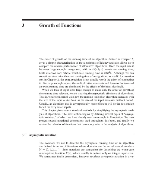
Abuse
sufficiently large n
In stead of writing “f(n)∈ (g(n))”, we write f(n) = (g(n))” to indicate that f(n) is a member of (g(n))
Asymptotic tight bound
bound, we use -notation.
f (n) ( g (n))
2 2
f (n) O( g (n)) f (n) ( g (n))
2 2
an bn c O(n ) an bn c (n )
Байду номын сангаасnotation(1)
– (g(n)) = {f (n) : there exist positive constants c and n0 such that 0 ≤ c g(n) ≤ f(n) for all n ≥ n0} . g(n) is an asymptotic lower bound for f(n). – Example: n = (lg n), with c=1 and n0 =16. – Examples of functions in (n² ): n² n² n, n² n, 1000n² 1000n, , + + 1000n² 1000n, Also, n³ n 2.0000 , n² lg lg n, , lg
1 2 c1n n 3n c2 n 2 2
2
1 3 0 c1 c2 , n n0 2 n
1 1 n 6 n0 7, c2 , c1 2 14
Continue
Intuitively, the lower-order terms of an asymptotically positive function can be ignored in determining asymptotically tight bound because they are insignificant for large n. The coefficient of the highest-order term can likewise be ignored, since it only changes c1 and c2 by a constant factor equal to the coefficient.
英语听课笔记范文10篇试卷讲解

英语听课笔记范文10篇试卷讲解Lecture Notes Template 1。
Title: Introduction to Artificial Intelligence.Lecturer: Dr. Emily Jones.Date: September 5, 2023。
Key Concepts:Artificial Intelligence (AI): The science of creating intelligent machines that can perform tasks typically requiring human intelligence.Machine Learning (ML): A subset of AI that allows computers to learn from data without explicit programming.Deep Learning (DL): A type of ML that uses artificial neural networks to process data and make predictions.Natural Language Processing (NLP): A field of AI focused on enabling computers to understand and generate human language.Computer Vision (CV): A field of AI that enables computers to analyze and understand images and videos.Lecture Outline:I. What is AI?Definition, scope, and applications.II. Types of AI.Narrow AI vs. General AI.Symbolic AI vs. Statistical AI.III. Machine Learning.Supervised, unsupervised, and reinforcement learning.Algorithms and techniques.IV. Deep Learning.Artificial neural networks.CNNs, RNNs, and LSTMs.V. NLP and CV.Text processing, machine translation, speech recognition.Image classification, object detection, facial recognition.Key Takeaways:AI is a rapidly growing field with the potential torevolutionize many industries.Machine learning and deep learning are fundamental techniques in AI.NLP and CV enable computers to interact with humans and the world in a more meaningful way.Lecture Notes Template 2。
算法导论习题答案 (1)
Introduction to Algorithms September 24, 2004Massachusetts Institute of Technology 6.046J/18.410J Professors Piotr Indyk and Charles E. Leiserson Handout 7Problem Set 1 SolutionsExercise 1-1. Do Exercise 2.3-7 on page 37 in CLRS.Solution:The following algorithm solves the problem:1.Sort the elements in S using mergesort.2.Remove the last element from S. Let y be the value of the removed element.3.If S is nonempty, look for z=x−y in S using binary search.4.If S contains such an element z, then STOP, since we have found y and z such that x=y+z.Otherwise, repeat Step 2.5.If S is empty, then no two elements in S sum to x.Notice that when we consider an element y i of S during i th iteration, we don’t need to look at the elements that have already been considered in previous iterations. Suppose there exists y j∗S, such that x=y i+y j. If j<i, i.e. if y j has been reached prior to y i, then we would have found y i when we were searching for x−y j during j th iteration and the algorithm would have terminated then.Step 1 takes �(n lg n)time. Step 2 takes O(1)time. Step 3 requires at most lg n time. Steps 2–4 are repeated at most n times. Thus, the total running time of this algorithm is �(n lg n). We can do a more precise analysis if we notice that Step 3 actually requires �(lg(n−i))time at i th iteration.However, if we evaluate �n−1lg(n−i), we get lg(n−1)!, which is �(n lg n). So the total runningi=1time is still �(n lg n).Exercise 1-2. Do Exercise 3.1-3 on page 50 in CLRS.Exercise 1-3. Do Exercise 3.2-6 on page 57 in CLRS.Exercise 1-4. Do Problem 3-2 on page 58 of CLRS.Problem 1-1. Properties of Asymptotic NotationProve or disprove each of the following properties related to asymptotic notation. In each of the following assume that f, g, and h are asymptotically nonnegative functions.� (a) f (n ) = O (g (n )) and g (n ) = O (f (n )) implies that f (n ) = �(g (n )).Solution:This Statement is True.Since f (n ) = O (g (n )), then there exists an n 0 and a c such that for all n √ n 0, f (n ) ←Similarly, since g (n )= O (f (n )), there exists an n � 0 and a c such that for allcg (n ). �f (n ). Therefore, for all n √ max(n 0,n Hence, f (n ) = �(g (n )).�()g n ,0← �),0c 1 � g (n ) ← f (n ) ← cg (n ).n √ n c � 0 (b) f (n ) + g (n ) = �(max(f (n ),g (n ))).Solution:This Statement is True.For all n √ 1, f (n ) ← max(f (n ),g (n )) and g (n ) ← max(f (n ),g (n )). Therefore:f (n ) +g (n ) ← max(f (n ),g (n )) + max(f (n ),g (n )) ← 2 max(f (n ),g (n ))and so f (n ) + g (n )= O (max(f (n ),g (n ))). Additionally, for each n , either f (n ) √max(f (n ),g (n )) or else g (n ) √ max(f (n ),g (n )). Therefore, for all n √ 1, f (n ) + g (n ) √ max(f (n ),g (n )) and so f (n ) + g (n ) = �(max(f (n ),g (n ))). Thus, f (n ) + g (n ) = �(max(f (n ),g (n ))).(c) Transitivity: f (n ) = O (g (n )) and g (n ) = O (h (n )) implies that f (n ) = O (h (n )).Solution:This Statement is True.Since f (n )= O (g (n )), then there exists an n 0 and a c such that for all n √ n 0, �)f ()n ,0← �()g n ,0← f (n ) ← cg (n ). Similarly, since g (n ) = O (h (n )), there exists an n �h (n ). Therefore, for all n √ max(n 0,n and a c � such thatfor all n √ n Hence, f (n ) = O (h (n )).cc�h (n ).c (d) f (n ) = O (g (n )) implies that h (f (n )) = O (h (g (n )).Solution:This Statement is False.We disprove this statement by giving a counter-example. Let f (n ) = n and g (n ) = 3n and h (n )=2n . Then h (f (n )) = 2n and h (g (n )) = 8n . Since 2n is not O (8n ), this choice of f , g and h is a counter-example which disproves the theorem.(e) f(n)+o(f(n))=�(f(n)).Solution:This Statement is True.Let h(n)=o(f(n)). We prove that f(n)+o(f(n))=�(f(n)). Since for all n√1, f(n)+h(n)√f(n), then f(n)+h(n)=�(f(n)).Since h(n)=o(f(n)), then there exists an n0such that for all n>n0, h(n)←f(n).Therefore, for all n>n0, f(n)+h(n)←2f(n)and so f(n)+h(n)=O(f(n)).Thus, f(n)+h(n)=�(f(n)).(f) f(n)=o(g(n))and g(n)=o(f(n))implies f(n)=�(g(n)).Solution:This Statement is False.We disprove this statement by giving a counter-example. Consider f(n)=1+cos(�≈n)and g(n)=1−cos(�≈n).For all even values of n, f(n)=2and g(n)=0, and there does not exist a c1for which f(n)←c1g(n). Thus, f(n)is not o(g(n)), because if there does not exist a c1 for which f(n)←c1g(n), then it cannot be the case that for any c1>0and sufficiently large n, f(n)<c1g(n).For all odd values of n, f(n)=0and g(n)=2, and there does not exist a c for which g(n)←cf(n). By the above reasoning, it follows that g(n)is not o(f(n)). Also, there cannot exist c2>0for which c2g(n)←f(n), because we could set c=1/c2if sucha c2existed.We have shown that there do not exist constants c1>0and c2>0such that c2g(n)←f(n)←c1g(n). Thus, f(n)is not �(g(n)).Problem 1-2. Computing Fibonacci NumbersThe Fibonacci numbers are defined on page 56 of CLRS asF0=0,F1=1,F n=F n−1+F n−2for n√2.In Exercise 1-3, of this problem set, you showed that the n th Fibonacci number isF n=�n−� n,�5where �is the golden ratio and �is its conjugate.A fellow 6.046 student comes to you with the following simple recursive algorithm for computing the n th Fibonacci number.F IB(n)1 if n=02 then return 03 elseif n=14 then return 15 return F IB(n−1)+F IB(n−2)This algorithm is correct, since it directly implements the definition of the Fibonacci numbers. Let’s analyze its running time. Let T(n)be the worst-case running time of F IB(n).1(a) Give a recurrence for T(n), and use the substitution method to show that T(n)=O(F n).Solution: The recurrence is: T(n)=T(n−1)+T(n−2)+1.We use the substitution method, inducting on n. Our Induction Hypothesis is: T(n)←cF n−b.To prove the inductive step:T(n)←cF n−1+cF n−2−b−b+1← cF n−2b+1Therefore, T(n)←cF n−b+1provided that b√1. We choose b=2and c=10.∗{For the base case consider n0,1}and note the running time is no more than10−2=8.(b) Similarly, show that T(n)=�(F n), and hence, that T(n)=�(F n).Solution: Again the recurrence is: T(n)=T(n−1)+T(n−2)+1.We use the substitution method, inducting on n. Our Induction Hypothesis is: T(n)√F n.To prove the inductive step:T(n)√F n−1+F n−2+1√F n+1Therefore, T(n)←F n. For the base case consider n∗{0,1}and note the runningtime is no less than 1.1In this problem, please assume that all operations take unit time. In reality, the time it takes to add two numbers depends on the number of bits in the numbers being added (more precisely, on the number of memory words). However, for the purpose of this problem, the approximation of unit time addition will suffice.Professor Grigori Potemkin has recently published an improved algorithm for computing the n th Fibonacci number which uses a cleverly constructed loop to get rid of one of the recursive calls. Professor Potemkin has staked his reputation on this new algorithm, and his tenure committee has asked you to review his algorithm.F IB�(n)1 if n=02 then return 03 elseif n=14 then return 15 6 7 8 sum �1for k�1to n−2do sum �sum +F IB�(k) return sumSince it is not at all clear that this algorithm actually computes the n th Fibonacci number, let’s prove that the algorithm is correct. We’ll prove this by induction over n, using a loop invariant in the inductive step of the proof.(c) State the induction hypothesis and the base case of your correctness proof.Solution: To prove the algorithm is correct, we are inducting on n. Our inductionhypothesis is that for all n<m, Fib�(n)returns F n, the n th Fibonacci number.Our base case is m=2. We observe that the first four lines of Potemkin guaranteethat Fib�(n)returns the correct value when n<2.(d) State a loop invariant for the loop in lines 6-7. Prove, using induction over k, that your“invariant” is indeed invariant.Solution: Our loop invariant is that after the k=i iteration of the loop,sum=F i+2.We prove this induction using induction over k. We assume that after the k=(i−1)iteration of the loop, sum=F i+1. Our base case is i=1. We observe that after thefirst pass through the loop, sum=2which is the 3rd Fibonacci number.To complete the induction step we observe that if sum=F i+1after the k=(i−1)andif the call to F ib�(i)on Line 7 correctly returns F i(by the induction hypothesis of ourcorrectness proof in the previous part of the problem) then after the k=i iteration ofthe loop sum=F i+2. This follows immediately form the fact that F i+F i+1=F i+2.(e) Use your loop invariant to complete the inductive step of your correctness proof.Solution: To complete the inductive step of our correctness proof, we must show thatif F ib�(n)returns F n for all n<m then F ib�(m)returns m. From the previous partwe know that if F ib�(n)returns F n for all n<m, then at the end of the k=i iterationof the loop sum=F i+2. We can thus conclude that after the k=m−2iteration ofthe loop, sum=F m which completes our correctness proof.(f) What is the asymptotic running time, T�(n), of F IB�(n)? Would you recommendtenure for Professor Potemkin?Solution: We will argue that T�(n)=�(F n)and thus that Potemkin’s algorithm,F ib�does not improve upon the assymptotic performance of the simple recurrsivealgorithm, F ib. Therefore we would not recommend tenure for Professor Potemkin.One way to see that T�(n)=�(F n)is to observe that the only constant in the programis the 1 (in lines 5 and 4). That is, in order for the program to return F n lines 5 and 4must be executed a total of F n times.Another way to see that T�(n)=�(F n)is to use the substitution method with thehypothesis T�(n)√F n and the recurrence T�(n)=cn+�n−2T�(k).k=1Problem 1-3. Polynomial multiplicationOne can represent a polynomial, in a symbolic variable x, with degree-bound n as an array P[0..n] of coefficients. Consider two linear polynomials, A(x)=a1x+a0and B(x)=b1x+b0, where a1, a0, b1, and b0are numerical coefficients, which can be represented by the arrays [a0,a1]and [b0,b1], respectively. We can multiply A and B using the four coefficient multiplicationsm1=a1·b1,m2=a1·b0,m3=a0·b1,m4=a0·b0,as well as one numerical addition, to form the polynomialC(x)=m1x2+(m2+m3)x+m4,which can be represented by the array[c0,c1,c2]=[m4,m3+m2,m1].(a) Give a divide-and-conquer algorithm for multiplying two polynomials of degree-bound n,represented as coefficient arrays, based on this formula.Solution:We can use this idea to recursively multiply polynomials of degree n−1, where n isa power of 2, as follows:Let p(x)and q(x)be polynomials of degree n−1, and divide each into the upper n/2 and lower n/2terms:p(x)=a(x)x n/2+b(x),q(x)=c(x)x n/2+d(x),where a(x), b(x), c(x), and d(x)are polynomials of degree n/2−1. The polynomial product is thenp(x)q(x)=(a(x)x n/2+b(x))(c(x)x n/2+d(x))=a(x)c(x)x n+(a(x)d(x)+b(x)c(x))x n/2+b(x)d(x).The four polynomial products a(x)c(x), a(x)d(x), b(x)c(x), and b(x)d(x)are computed recursively.(b) Give and solve a recurrence for the worst-case running time of your algorithm.Solution:Since we can perform the dividing and combining of polynomials in time �(n), recursive polynomial multiplication gives us a running time ofT(n)=4T(n/2)+�(n)=�(n2).(c) Show how to multiply two linear polynomials A(x)=a1x+a0and B(x)=b1x+b0using only three coefficient multiplications.Solution:We can use the following 3 multiplications:m1=(a+b)(c+d)=ac+ad+bc+bd,m2=ac,m3=bd,so the polynomial product is(ax+b)(cx+d)=m2x2+(m1−m2−m3)x+m3.� (d) Give a divide-and-conquer algorithm for multiplying two polynomials of degree-bound nbased on your formula from part (c).Solution:The algorithm is the same as in part (a), except for the fact that we need only compute three products of polynomials of degree n/2 to get the polynomial product.(e) Give and solve a recurrence for the worst-case running time of your algorithm.Solution:Similar to part (b):T (n )=3T (n/2) + �(n )lg 3)= �(n �(n 1.585)Alternative solution Instead of breaking a polynomial p (x ) into two smaller polynomials a (x ) and b (x ) such that p (x )= a (x ) + x n/2b (x ), as we did above, we could do the following:Collect all the even powers of p (x ) and substitute y = x 2 to create the polynomial a (y ). Then collect all the odd powers of p (x ), factor out x and substitute y = x 2 to create the second polynomial b (y ). Then we can see thatp (x ) = a (y ) + x b (y )· Both a (y ) and b (y ) are polynomials of (roughly) half the original size and degree, and we can proceed with our multiplications in a way analogous to what was done above.Notice that, at each level k , we need to compute y k = y 2 (where y 0 = x ), whichk −1 takes time �(1) per level and does not affect the asymptotic running time.。
data structures and algorithm analysi英文原版 pdf (2)

data structures and algorithm analysi英文原版 pdfTitle: Data Structures and Algorithm Analysis: A Comprehensive ReviewIntroduction:Data structures and algorithm analysis are fundamental concepts in computer science. They form the backbone of efficient and optimized software development. This article aims to provide a comprehensive review of the book "Data Structures and Algorithm Analysis" in its English original version PDF format. The review will cover the key points, structure, and significance of the book.I. Overview of the Book:1.1 Importance of Data Structures:- Discuss the significance of data structures in organizing and manipulating data efficiently.- Explain how data structures enhance the performance and scalability of software applications.1.2 Algorithm Analysis:- Describe the role of algorithm analysis in evaluating the efficiency and performance of algorithms.- Highlight the importance of selecting appropriate algorithms for different problem-solving scenarios.1.3 Book Structure:- Outline the organization of the book, including chapters, sections, and topics covered.- Emphasize the logical progression of concepts, starting from basic data structures to advanced algorithm analysis.II. Data Structures:2.1 Arrays and Linked Lists:- Explain the characteristics, advantages, and disadvantages of arrays and linked lists.- Discuss the implementation details, operations, and time complexities of these data structures.2.2 Stacks and Queues:- Define stacks and queues and their applications in various scenarios.- Elaborate on the implementation, operations, and time complexities of stacks and queues.2.3 Trees and Graphs:- Introduce the concepts of trees and graphs and their real-world applications.- Discuss different types of trees (binary, AVL, B-trees) and graphs (directed, undirected, weighted).III. Algorithm Analysis:3.1 Asymptotic Notation:- Explain the significance of asymptotic notation in analyzing the efficiency of algorithms.- Discuss the Big-O, Omega, and Theta notations and their usage in algorithm analysis.3.2 Sorting and Searching Algorithms:- Describe various sorting algorithms such as bubble sort, insertion sort, merge sort, and quicksort.- Discuss searching algorithms like linear search, binary search, and hash-based searching.3.3 Dynamic Programming and Greedy Algorithms:- Define dynamic programming and greedy algorithms and their applications.- Provide examples of problems that can be solved using these approaches.IV. Advanced Topics:4.1 Hashing and Hash Tables:- Explain the concept of hashing and its applications in efficient data retrieval.- Discuss hash functions, collision handling, and the implementation of hash tables.4.2 Graph Algorithms:- Explore advanced graph algorithms such as Dijkstra's algorithm, breadth-first search, and depth-first search.- Discuss their applications in solving complex problems like shortest path finding and network analysis.4.3 Advanced Data Structures:- Introduce advanced data structures like heaps, priority queues, and self-balancing binary search trees.- Explain their advantages, implementation details, and usage in various scenarios.V. Summary:5.1 Key Takeaways:- Summarize the main points covered in the book, emphasizing the importance of data structures and algorithm analysis.- Highlight the significance of selecting appropriate data structures and algorithms for efficient software development.5.2 Practical Applications:- Discuss real-world scenarios where the concepts from the book can be applied.- Illustrate how understanding data structures and algorithm analysis can lead to optimized software solutions.5.3 Conclusion:- Conclude the review by emphasizing the relevance and usefulness of the book "Data Structures and Algorithm Analysis."- Encourage readers to explore the book further for a deeper understanding of the subject.In conclusion, "Data Structures and Algorithm Analysis" is a comprehensive guide that covers essential concepts in data structures and algorithm analysis. The book's structure, detailed explanations, and practical examples make it a valuable resource for computer science students, software developers, and anyone interested in optimizing their software solutions. Understanding these fundamental concepts is crucial for building efficient and scalable software applications.。
2算法性能的渐近函数algorithm-analysis-basic
3Growth of FunctionsThe order of growth of the running time of an algorithm,defined in Chapter2,gives a simple characterization of the algorithm’s efficiency and also allows us tocompare the relative performance of alternative algorithms.Once the input size nbecomes large enough,merge sort,with its‚.n lg n/worst-case running time,beats insertion sort,whose worst-case running time is‚.n2/.Although we cansometimes determine the exact running time of an algorithm,as we did for insertionsort in Chapter2,the extra precision is not usually worth the effort of computingit.For large enough inputs,the multiplicative constants and lower-order terms ofan exact running time are dominated by the effects of the input size itself.When we look at input sizes large enough to make only the order of growth ofthe running time relevant,we are studying the asymptotic efficiency of algorithms.That is,we are concerned with how the running time of an algorithm increases withthe size of the input in the limit,as the size of the input increases without bound.Usually,an algorithm that is asymptotically more efficient will be the best choicefor all but very small inputs.This chapter gives several standard methods for simplifying the asymptotic anal-ysis of algorithms.The next section begins by defining several types of“asymp-totic notation,”of which we have already seen an example in‚-notation.We thenpresent several notational conventions used throughout this book,andfinally wereview the behavior of functions that commonly arise in the analysis of algorithms.3.1Asymptotic notationThe notations we use to describe the asymptotic running time of an algorithmare defined in terms of functions whose domains are the set of natural numbersN D f0;1;2;:::g.Such notations are convenient for describing the worst-caserunning-time function T.n/,which usually is defined only on integer input sizes.We sometimesfind it convenient,however,to abuse asymptotic notation in a va-44Chapter3Growth of Functionsriety of ways.For example,we might extend the notation to the domain of realnumbers or,alternatively,restrict it to a subset of the natural numbers.We shouldmake sure,however,to understand the precise meaning of the notation so that whenwe abuse,we do not misuse it.This section defines the basic asymptotic notationsand also introduces some common abuses.Asymptotic notation,functions,and running timesWe will use asymptotic notation primarily to describe the running times of algo-rithms,as when we wrote that insertion sort’s worst-case running time is‚.n2/.Asymptotic notation actually applies to functions,however.Recall that we charac-terized insertion sort’s worst-case running time as an2C bn C c,for some constantsa,b,and c.By writing that insertion sort’s running time is‚.n2/,we abstractedaway some details of this function.Because asymptotic notation applies to func-tions,what we were writing as‚.n2/was the function an2C bn C c,which inthat case happened to characterize the worst-case running time of insertion sort.In this book,the functions to which we apply asymptotic notation will usuallycharacterize the running times of algorithms.But asymptotic notation can apply tofunctions that characterize some other aspect of algorithms(the amount of spacethey use,for example),or even to functions that have nothing whatsoever to dowith algorithms.Even when we use asymptotic notation to apply to the running time of an al-gorithm,we need to understand which running time we mean.Sometimes we areinterested in the worst-case running time.Often,however,we wish to characterizethe running time no matter what the input.In other words,we often wish to makea blanket statement that covers all inputs,not just the worst case.We shall seeasymptotic notations that are well suited to characterizing running times no matterwhat the input.‚-notationIn Chapter2,we found that the worst-case running time of insertion sort isT.n/D‚.n2/.Let us define what this notation means.For a given function g.n/,we denote by‚.g.n//the set of functions‚.g.n//D f f.n/W there exist positive constants c1,c2,and n0such that0Äc1g.n/Äf.n/Äc2g.n/for all n n0g:11Within set notation,a colon means“such that.”3.1Asymptotic notation 45(b)(c)(a)n n n n 0n 0n 0 f.n/D ‚.g.n//f.n/D O.g.n// f.n/D .g.n//f.n/f.n/f.n/cg.n/cg.n/c 1g.n/c 2g.n/Figure 3.1Graphic examples of the ‚,O ,and notations.In each part,the value of n 0shown is the minimum possible value;any greater value would also work.(a)‚-notation bounds a func-tion to within constant factors.We write f.n/D ‚.g.n//if there exist positive constants n 0,c 1,and c 2such that at and to the right of n 0,the value of f.n/always lies between c 1g.n/and c 2g.n/inclusive.(b)O -notation gives an upper bound for a function to within a constant factor.We write f.n/D O.g.n//if there are positive constants n 0and c such that at and to the right of n 0,the value of f.n/always lies on or below cg.n/.(c) -notation gives a lower bound for a function to within a constant factor.We write f.n/D .g.n//if there are positive constants n 0and c such that at and to the right of n 0,the value of f.n/always lies on or above cg.n/.A function f.n/belongs to the set ‚.g.n//if there exist positive constants c 1and c 2such that it can be “sandwiched”between c 1g.n/and c 2g.n/,for suffi-ciently large n .Because ‚.g.n//is a set,we could write “f.n/2‚.g.n//”to indicate that f.n/is a member of ‚.g.n//.Instead,we will usually write “f.n/D ‚.g.n//”to express the same notion.You might be confused because we abuse equality in this way,but we shall see later in this section that doing so has its advantages.Figure 3.1(a)gives an intuitive picture of functions f.n/and g.n/,where f.n/D ‚.g.n//.For all values of n at and to the right of n 0,the value of f.n/lies at or above c 1g.n/and at or below c 2g.n/.In other words,for all n n 0,the function f.n/is equal to g.n/to within a constant factor.We say that g.n/is an asymptotically tight bound for f.n/.The definition of ‚.g.n//requires that every member f.n/2‚.g.n//be asymptotically nonnegative ,that is,that f.n/be nonnegative whenever n is suf-ficiently large.(An asymptotically positive function is one that is positive for all sufficiently large n .)Consequently,the function g.n/itself must be asymptotically nonnegative,or else the set ‚.g.n//is empty.We shall therefore assume that every function used within ‚-notation is asymptotically nonnegative.This assumption holds for the other asymptotic notations defined in this chapter as well.46Chapter 3Growth of FunctionsIn Chapter 2,we introduced an informal notion of ‚-notation that amounted to throwing away lower-order terms and ignoring the leading coefficient of the highest-order term.Let us briefly justify this intuition by using the formal defi-nition to show that 12n 2 3n D ‚.n 2/.To do so,we must determine positive constants c 1,c 2,and n 0such thatc 1n 2Ä12n 2 3n Äc 2n 2for all n n 0.Dividing by n 2yieldsc 1Ä12 3nÄc 2:We can make the right-hand inequality hold for any value of n 1by choosing any constant c 2 1=2.Likewise,we can make the left-hand inequality hold for any value of n 7by choosing any constant c 1Ä1=14.Thus,by choosing c 1D 1=14,c 2D 1=2,and n 0D 7,we can verify that 12n 2 3n D ‚.n 2/.Certainly,other choices for the constants exist,but the important thing is that some choice exists.Note that these constants depend on the function 12n 2 3n ;a different function belonging to ‚.n 2/would usually require different constants.We can also use the formal definition to verify that 6n 3¤‚.n 2/.Suppose for the purpose of contradiction that c 2and n 0exist such that 6n 3Äc 2n 2for all n n 0.But then dividing by n 2yields n Äc 2=6,which cannot possibly hold for arbitrarily large n ,since c 2is constant.Intuitively,the lower-order terms of an asymptotically positive function can be ignored in determining asymptotically tight bounds because they are insignificant for large n .When n is large,even a tiny fraction of the highest-order term suf-fices to dominate the lower-order terms.Thus,setting c 1to a value that is slightly smaller than the coefficient of the highest-order term and setting c 2to a value that is slightly larger permits the inequalities in the definition of ‚-notation to be sat-isfied.The coefficient of the highest-order term can likewise be ignored,since it only changes c 1and c 2by a constant factor equal to the coefficient.As an example,consider any quadratic function f.n/D an 2C bn C c ,where a ,b ,and c are constants and a >0.Throwing away the lower-order terms and ignoring the constant yields f.n/D ‚.n 2/.Formally,to show the same thing,we take the constants c 1D a=4,c 2D 7a=4,and n 0D 2 max .j b j =a;p j c j =a/.You may verify that 0Äc 1n 2Äan 2C bn C c Äc 2n 2for all n n 0.In general,for any polynomial p.n/D P d i D 0a i n i ,where the a i are constants and a d >0,we have p.n/D ‚.n d /(see Problem 3-1).Since any constant is a degree-0polynomial,we can express any constant func-tion as ‚.n 0/,or ‚.1/.This latter notation is a minor abuse,however,because the3.1Asymptotic notation47 expression does not indicate what variable is tending to infinity.2We shall often use the notation‚.1/to mean either a constant or a constant function with respect to some variable.O-notationThe‚-notation asymptotically bounds a function from above and below.When we have only an asymptotic upper bound,we use O-notation.For a given func-tion g.n/,we denote by O.g.n//(pronounced“big-oh of g of n”or sometimes just“oh of g of n”)the set of functionsO.g.n//D f f.n/W there exist positive constants c and n0such that0Äf.n/Äcg.n/for all n n0g:We use O-notation to give an upper bound on a function,to within a constant factor.Figure3.1(b)shows the intuition behind O-notation.For all values n at and to the right of n0,the value of the function f.n/is on or below cg.n/.We write f.n/D O.g.n//to indicate that a function f.n/is a member of the set O.g.n//.Note that f.n/D‚.g.n//implies f.n/D O.g.n//,since‚-notation is a stronger notion than O-notation.Written set-theoretically,we have ‚.g.n//ÂO.g.n//.Thus,our proof that any quadratic function an2C bn C c, where a>0,is in‚.n2/also shows that any such quadratic function is in O.n2/. What may be more surprising is that when a>0,any linear function an C b is in O.n2/,which is easily verified by taking c D a C j b j and n0D max.1; b=a/. If you have seen O-notation before,you mightfind it strange that we should write,for example,n D O.n2/.In the literature,we sometimesfind O-notation informally describing asymptotically tight bounds,that is,what we have defined using‚-notation.In this book,however,when we write f.n/D O.g.n//,we are merely claiming that some constant multiple of g.n/is an asymptotic upper bound on f.n/,with no claim about how tight an upper bound it is.Distinguish-ing asymptotic upper bounds from asymptotically tight bounds is standard in the algorithms literature.Using O-notation,we can often describe the running time of an algorithm merely by inspecting the algorithm’s overall structure.For example,the doubly nested loop structure of the insertion sort algorithm from Chapter2immediately yields an O.n2/upper bound on the worst-case running time:the cost of each it-eration of the inner loop is bounded from above by O.1/(constant),the indices i2The real problem is that our ordinary notation for functions does not distinguish functions from values.In -calculus,the parameters to a function are clearly specified:the function n2could be written as n:n2,or even r:r2.Adopting a more rigorous notation,however,would complicate algebraic manipulations,and so we choose to tolerate the abuse.48Chapter3Growth of Functionsand j are both at most n,and the inner loop is executed at most once for each ofthe n2pairs of values for i and j.Since O-notation describes an upper bound,when we use it to bound the worst-case running time of an algorithm,we have a bound on the running time of the algo-rithm on every input—the blanket statement we discussed earlier.Thus,the O.n2/bound on worst-case running time of insertion sort also applies to its running timeon every input.The‚.n2/bound on the worst-case running time of insertion sort,however,does not imply a‚.n2/bound on the running time of insertion sort onevery input.For example,we saw in Chapter2that when the input is alreadysorted,insertion sort runs in‚.n/time.Technically,it is an abuse to say that the running time of insertion sort is O.n2/,since for a given n,the actual running time varies,depending on the particularinput of size n.When we say“the running time is O.n2/,”we mean that there is afunction f.n/that is O.n2/such that for any value of n,no matter what particularinput of size n is chosen,the running time on that input is bounded from above bythe value f.n/.Equivalently,we mean that the worst-case running time is O.n2/.-notationJust as O-notation provides an asymptotic upper bound on a function, -notationprovides an asymptotic lower bound.For a given function g.n/,we denoteby .g.n//(pronounced“big-omega of g of n”or sometimes just“omega of gof n”)the set of functions.g.n//D f f.n/W there exist positive constants c and n0such that0Äcg.n/Äf.n/for all n n0g:Figure3.1(c)shows the intuition behind -notation.For all values n at or to theright of n0,the value of f.n/is on or above cg.n/.From the definitions of the asymptotic notations we have seen thus far,it is easyto prove the following important theorem(see Exercise3.1-5).Theorem3.1For any two functions f.n/and g.n/,we have f.n/D‚.g.n//if and only iff.n/D O.g.n//and f.n/D .g.n//.As an example of the application of this theorem,our proof that an2C bn C c D‚.n2/for any constants a,b,and c,where a>0,immediately implies thatan2C bn C c D .n2/and an2C bn C c D O.n2/.In practice,rather than usingTheorem3.1to obtain asymptotic upper and lower bounds from asymptoticallytight bounds,as we did for this example,we usually use it to prove asymptoticallytight bounds from asymptotic upper and lower bounds.3.1Asymptotic notation49 When we say that the running time(no modifier)of an algorithm is .g.n//, we mean that no matter what particular input of size n is chosen for each value of n,the running time on that input is at least a constant times g.n/,for sufficiently large n.Equivalently,we are giving a lower bound on the best-case running time of an algorithm.For example,the best-case running time of insertion sort is .n/, which implies that the running time of insertion sort is .n/.The running time of insertion sort therefore belongs to both .n/and O.n2/, since it falls anywhere between a linear function of n and a quadratic function of n. Moreover,these bounds are asymptotically as tight as possible:for instance,the running time of insertion sort is not .n2/,since there exists an input for which insertion sort runs in‚.n/time(e.g.,when the input is already sorted).It is not contradictory,however,to say that the worst-case running time of insertion sort is .n2/,since there exists an input that causes the algorithm to take .n2/time. Asymptotic notation in equations and inequalitiesWe have already seen how asymptotic notation can be used within mathematical formulas.For example,in introducing O-notation,we wrote“n D O.n2/.”We might also write2n2C3n C1D2n2C‚.n/.How do we interpret such formulas? When the asymptotic notation stands alone(that is,not within a larger formula) on the right-hand side of an equation(or inequality),as in n D O.n2/,we have already defined the equal sign to mean set membership:n2O.n2/.In general, however,when asymptotic notation appears in a formula,we interpret it as stand-ing for some anonymous function that we do not care to name.For example,the formula2n2C3n C1D2n2C‚.n/means that2n2C3n C1D2n2C f.n/, where f.n/is some function in the set‚.n/.In this case,we let f.n/D3n C1, which indeed is in‚.n/.Using asymptotic notation in this manner can help eliminate inessential detail and clutter in an equation.For example,in Chapter2we expressed the worst-case running time of merge sort as the recurrenceT.n/D2T.n=2/C‚.n/:If we are interested only in the asymptotic behavior of T.n/,there is no point in specifying all the lower-order terms exactly;they are all understood to be included in the anonymous function denoted by the term‚.n/.The number of anonymous functions in an expression is understood to be equal to the number of times the asymptotic notation appears.For example,in the ex-pressionXnO.i/;i D150Chapter3Growth of Functionsthere is only a single anonymous function(a function of i).This expression is thusnot the same as O.1/C O.2/C C O.n/,which doesn’t really have a cleaninterpretation.In some cases,asymptotic notation appears on the left-hand side of an equation,as in2n2C‚.n/D‚.n2/:We interpret such equations using the following rule:No matter how the anony-mous functions are chosen on the left of the equal sign,there is a way to choosethe anonymous functions on the right of the equal sign to make the equation valid.Thus,our example means that for any function f.n/2‚.n/,there is some func-tion g.n/2‚.n2/such that2n2C f.n/D g.n/for all n.In other words,theright-hand side of an equation provides a coarser level of detail than the left-handside.We can chain together a number of such relationships,as in2n2C3n C1D2n2C‚.n/D‚.n2/:We can interpret each equation separately by the rules above.Thefirst equa-tion says that there is some function f.n/2‚.n/such that2n2C3n C1D2n2C f.n/for all n.The second equation says that for any function g.n/2‚.n/(such as the f.n/just mentioned),there is some function h.n/2‚.n2/suchthat2n2C g.n/D h.n/for all n.Note that this interpretation implies that2n2C3n C1D‚.n2/,which is what the chaining of equations intuitively givesus.o-notationThe asymptotic upper bound provided by O-notation may or may not be asymp-totically tight.The bound2n2D O.n2/is asymptotically tight,but the bound2n D O.n2/is not.We use o-notation to denote an upper bound that is not asymp-totically tight.We formally define o.g.n//(“little-oh of g of n”)as the seto.g.n//D f f.n/W for any positive constant c>0,there exists a constantn0>0such that0Äf.n/<cg.n/for all n n0g:For example,2n D o.n2/,but2n2¤o.n2/.The definitions of O-notation and o-notation are similar.The main differenceis that in f.n/D O.g.n//,the bound0Äf.n/Äcg.n/holds for some con-stant c>0,but in f.n/D o.g.n//,the bound0Äf.n/<cg.n/holds for allconstants c>0.Intuitively,in o-notation,the function f.n/becomes insignificantrelative to g.n/as n approaches infinity;that is,3.1Asymptotic notation51lim n!1f.n/g.n/D0:(3.1)Some authors use this limit as a definition of the o-notation;the definition in this book also restricts the anonymous functions to be asymptotically nonnegative.!-notationBy analogy,!-notation is to -notation as o-notation is to O-notation.We use !-notation to denote a lower bound that is not asymptotically tight.One way to define it is byf.n/2!.g.n//if and only if g.n/2o.f.n//:Formally,however,we define!.g.n//(“little-omega of g of n”)as the set!.g.n//D f f.n/W for any positive constant c>0,there exists a constantn0>0such that0Äcg.n/<f.n/for all n n0g:For example,n2=2D!.n/,but n2=2¤!.n2/.The relation f.n/D!.g.n// implies thatlim n!1f.n/g.n/D1;if the limit exists.That is,f.n/becomes arbitrarily large relative to g.n/as n approaches infinity.Comparing functionsMany of the relational properties of real numbers apply to asymptotic comparisons as well.For the following,assume that f.n/and g.n/are asymptotically positive. Transitivity:f.n/D‚.g.n//and g.n/D‚.h.n//imply f.n/D‚.h.n//;f.n/D O.g.n//and g.n/D O.h.n//imply f.n/D O.h.n//;f.n/D .g.n//and g.n/D .h.n//imply f.n/D .h.n//;f.n/D o.g.n//and g.n/D o.h.n//imply f.n/D o.h.n//;f.n/D!.g.n//and g.n/D!.h.n//imply f.n/D!.h.n//:Reflexivity:f.n/D‚.f.n//;f.n/D O.f.n//;f.n/D .f.n//:52Chapter3Growth of FunctionsSymmetry:f.n/D‚.g.n//if and only if g.n/D‚.f.n//:Transpose symmetry:f.n/D O.g.n//if and only if g.n/D .f.n//;f.n/D o.g.n//if and only if g.n/D!.f.n//:Because these properties hold for asymptotic notations,we can draw an analogybetween the asymptotic comparison of two functions f and g and the comparisonof two real numbers a and b:f.n/D O.g.n//is like aÄb;f.n/D .g.n//is like a b;f.n/D‚.g.n//is like a D b;f.n/D o.g.n//is like a<b;f.n/D!.g.n//is like a>b:We say that f.n/is asymptotically smaller than g.n/if f.n/D o.g.n//,and f.n/is asymptotically larger than g.n/if f.n/D!.g.n//.One property of real numbers,however,does not carry over to asymptotic nota-tion:Trichotomy:For any two real numbers a and b,exactly one of the following must hold:a<b,a D b,or a>b.Although any two real numbers can be compared,not all functions are asymptot-ically comparable.That is,for two functions f.n/and g.n/,it may be the casethat neither f.n/D O.g.n//nor f.n/D .g.n//holds.For example,we cannotcompare the functions n and n1C sin n using asymptotic notation,since the value ofthe exponent in n1C sin n oscillates between0and2,taking on all values in between.Exercises3.1-1Let f.n/and g.n/be asymptotically nonnegative ing the basic defi-nition of‚-notation,prove that max.f.n/;g.n//D‚.f.n/C g.n//.3.1-2Show that for any real constants a and b,where b>0,.n C a/b D‚.n b/:(3.2)3.2Standard notations and common functions533.1-3Explain why the statement,“The running time of algorithm A is at least O.n2/,”ismeaningless.3.1-4Is2n C1D O.2n/?Is22n D O.2n/?3.1-5Prove Theorem3.1.3.1-6Prove that the running time of an algorithm is‚.g.n//if and only if its worst-caserunning time is O.g.n//and its best-case running time is .g.n//.3.1-7Prove that o.g.n//\!.g.n//is the empty set.3.1-8We can extend our notation to the case of two parameters n and m that can go toinfinity independently at different rates.For a given function g.n;m/,we denoteby O.g.n;m//the set of functionsO.g.n;m//D f f.n;m/W there exist positive constants c,n0,and m0such that0Äf.n;m/Äcg.n;m/for all n n0or m m0g:Give corresponding definitions for .g.n;m//and‚.g.n;m//.3.2Standard notations and common functionsThis section reviews some standard mathematical functions and notations and ex-plores the relationships among them.It also illustrates the use of the asymptoticnotations.MonotonicityA function f.n/is monotonically increasing if mÄn implies f.m/Äf.n/.Similarly,it is monotonically decreasing if mÄn implies f.m/ f.n/.Afunction f.n/is strictly increasing if m<n implies f.m/<f.n/and strictlydecreasing if m<n implies f.m/>f.n/.。
麻省理工学院-算法导论
麻省理工学院-算法导论关于课本的介绍如下:本书自第一版出版以来,已经成为世界范围内广泛使用的大学教材和专业人员的标准参考手册。
本书全面论述了算法的内容,从一定深度上涵盖了算法的诸多方面,同时其讲授和分析方法又兼顾了各个层次读者的接受能力。
各章内容自成体系,可作为独立单元学习。
所有算法都用英文和伪码描述,使具备初步编程经验的人也可读懂。
全书讲解通俗易懂,且不失深度和数学上的严谨性。
第二版增加了新的章节,如算法作用、概率分析与随机算法、线性编程等,几乎对第一版的各个部分都作了大量修订。
学过计算机的都知道,这本书是全世界最权威的算法课程的大学课本了,基本上全世界的名牌大学用的教材都是它。
这本书一共四位作者,Thomas H. Cormen,Charles E. Leiserson和Ronald L. Rivest是来自MIT的教授,Clifford Stein是MIT出来的博士,现在哥伦比亚大学做教授,四人姓氏的首字母联在一起即是此书的英文简称(CLRS 2e),其中的第三作者Ronald L. Rivest是RSA算法的老大(算法名字里面的R即是指他),四个超级大牛出的一本书,此书不看人生不能算完整。
再介绍一下课堂录像里面授课的两位MIT的老师,第一位,外表“绝顶聪明”的,是本书的第二作者Charles E. Leiserson,以逻辑严密,风趣幽默享誉MIT。
第二位,留着金黄色的络腮胡子和马尾发的酷哥是Erik Demaine,21岁即取得MIT教授资格的天才,1981出生,今年才25岁,业余爱好是俄罗斯方块、演戏、琉璃、折纸、杂耍、魔术和结绳游戏。
另外,附上该书的中文电子版,pdg转pdf格式,中文版翻译自该书的第一版,中文书名没有使用《算法导论》,而使用的是《现代计算机常用数据结构和算法》,1994年出版时没有得到国外的授权,属于“私自翻译出版”,译者是南京大学计算机系的潘金贵。
课程重点算法导论是麻省理工学院电机工程与计算机科学系“理论计算机科学”集中选修课程的先导科目。
算法设计技巧与分析英文版课程设计 (2)

Algorithm Design Techniques and Analysis Course Design(English Version)IntroductionAlgorithm design is an essential component of computer science. Whether you are designing a new application ortrying to optimize an existing one, the ability to develop efficient algorithms can significantly impact performance, scalability, and user experience. The Algorithm Design Techniques and Analysis course is designed to provide insight into the core principles and methods of algorithm design, as well as the techniques and tools necessary for algorithm analysis.Course ObjectivesThe primary objective of this course is to enhance students’ ability to develop and analyze algorithms effectively. By the end of this course, students should be able to:•Understand the importance of algorithm design and analysis in computer science;•Employ a systematic approach to the design and analysis of algorithms;•Analyze algorithms for their time and space complexity;•Understand the difference between worst-case and average-case analysis;•Apply various algorithm design techniques to solve common problems, such as searching, sorting, and graph traversal;•Develop efficient implementations of algorithms using programming languages;•Apply the principles of algorithm design and analysis to real-world problems.Course OutlineWeek 1: Introduction to Algorithm Design and Analysis •Importance of algorithm design and analysis in computer science;•The role of algorithms in modern computing;•Overview of algorithm design techniques and analysis.Week 2: Algorithm Analysis•The basics of algorithm analysis;•Time and space complexity;•Worst-case and average-case analysis;•Asymptotic notation (Big O, Big Omega, Big Theta).Week 3: Algorithm Design Techniques - Searching and Sorting•Sequential search;•Binary search;•Bubble sort;•Selection sort;•Insertion sort;•Quick sort;•Merge sort.Week 4: Algorithm Design Techniques - Graph Traversal •Breadth-First Search (BFS);•Depth-First Search (DFS);•Shortest path algorithms (Dijkstra’s and Floyd-Warshall);•Minimum spanning tree algorithms (Prim’s and Kruskal’s).Week 5: Dynamic Programming•Principles of dynamic programming;•Top-down and bottom-up approaches;•Knapsack problem;•Longest Common Subsequence (LCS);•Longest Increasing Subsequence (LIS);•Matrix Chn Multiplication.Week 6: Greedy Algorithms•Principles of greedy algorithms;•Huffman coding;•Activity selection problem;•Kruskal’s algorithm for Minimum Spanning Trees;•Dijkstra’s algorithm for Shortest Paths.Week 7: Divide and Conquer•Principles of divide and conquer;•Binary search;•Merge sort;•Quicksort;•Maximum Subarray problem.Week 8: Final Projects•Apply the principles of algorithm design and analysis to real-world problems;•Develop efficient algorithms to solve the problem;•Analyze and optimize the performance of the algorithms.Course FormatThis course will consist of eight weeks of online lectures, discussion forums, and assignments. Each week, students will be provided with multimedia lectures, reading materials, and programming assignments. Students will be expected to engagein discussion forums and submit weekly assignments to demonstrate comprehension of the material. In the final week, students will be required to complete a final project, which will be graded based on the design and efficiency of their algorithm, as well as their ability to analyze and optimizeits performance.ConclusionThe Algorithm Design Techniques and Analysis course is intended to provide students with the fundamental principles and techniques of algorithm design and analysis. With this knowledge, students will be better equipped to developefficient algorithms for solving real-world problems. By the end of this course, students should have a solid foundationin algorithm design and analysis, enabling them to understand and develop optimized algorithms for a variety of applications.。
chap04-new算法
Several Points
Making good guess Avoiding pitfalls Changing variables
lg n T (n) 2T n n 2m m lg n T (2m ) 2T (2m /2 ) m S (m) T (2m ) S (m) 2 S (m / 2) m S (m) O(m lg m) T (n) S (m) O(lg n lg lg n)
Chapter 4. Recurrences
Outline
Offers three methods for solving recurrences, that is for obtaining asymptotic bounds on the solution In the substitution method, we guess a bound and then use mathematical induction to prove our guess correct The recursion-tree method converts the recurrence into a tree whose nodes represent the costs incurred at various levels The master method provides bounds for the recurrence of the form T (n) aT (n / b) f (n)
The Substitution method
T(n) = 2T(n/2) + n Guess: T(n) = O(n lg n) Proof: Prove that T(n) c n lg n for c>0 Assume T(n/2) c(n/2)lg(n/2) for some positive constant c then T(n) 2(c n/2 lg n/2) + n = cn lg n – cn + n cn lg n if c 1
《算法导论》习题答案
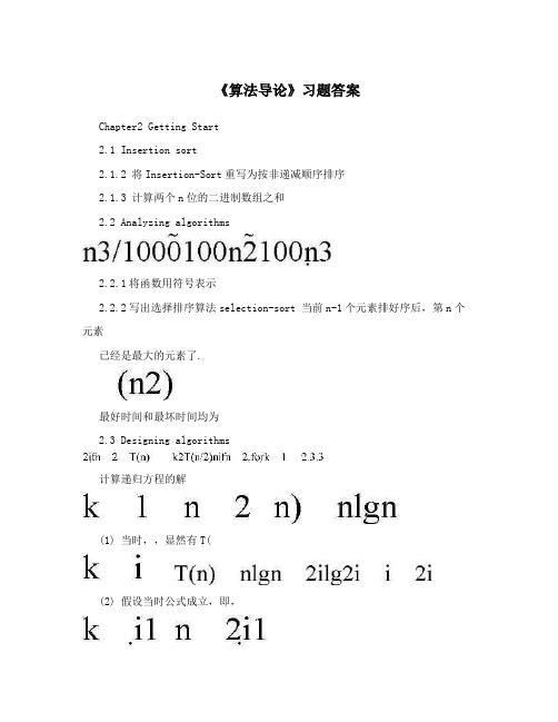
《算法导论》习题答案Chapter2 Getting Start2.1 Insertion sort2.1.2 将Insertion-Sort重写为按非递减顺序排序2.1.3 计算两个n位的二进制数组之和2.2 Analyzing algorithms2.2.1将函数用符号表示2.2.2写出选择排序算法selection-sort 当前n-1个元素排好序后,第n个元素已经是最大的元素了.最好时间和最坏时间均为2.3 Designing algorithms计算递归方程的解(1) 当时,,显然有T((2) 假设当时公式成立,即,则当,即时,2.3.4 给出insertion sort的递归版本的递归式2.3-6 使用二分查找来替代insertion-sort中while循环j?n;if A[i]+A[j]<xi?i+1elsej?j-1if A[i]+A[j]=xreturn trueelsereturn false时间复杂度为。
或者也可以先固定一个元素然后去二分查找x减去元素的差,复杂度为。
Chapter3 Growth of functions3.1Asymptotic notation3.1.2证明对于b时,对于,时,存在,当时,对于,3.1-4 判断与22n是否等于O(2n)3.1.6 证明如果算法的运行时间为,如果其最坏运行时间为O(g(n)),最佳运行时间为。
最坏时间O(g(n)),即;最佳时间,即3.1.7:证明定义3.2 Standard notation and common functions 3.2.2 证明证明当n>4时,,是否多项式有界~与设lgn=m,则?lgn~不是多项式有界的。
mememmmm2设,,是多项式有界的3.2.5比较lg(lg*n)与lg*(lgn)lg*(lgn)= lg*n-1设lg*n=x,lgx<x-1较大。
高等应用数学新答案
;
(2)
是一阶小量,不是二阶小量;
(3) /StabilityMatrix.html
4 定义为
,且假设 是正小量。忽略 的高次项,找到二次方
程较大根的近似值。推出增长得最快的扰动的波长的近似值。
提示:(部分符号已作修改!做作业时要把下面省略的详细步骤补充完整!)
实际上,这个解题过程相当繁琐,原因是它一开始就将一级近似代入方程推导,
我们前面提供的方法有效地避免了这一复杂性,希望引起大家的重视。
先简要提炼一下这份参考答案的解题过程:(最烦的方法,吃力不讨好!)
解的形式:
一级近似: Taylor 展开:
则:
方程左边:(太复杂略去) 方程右边:(太复杂略去) 相应项相等:
所以: 两个相继的近日点之间的角度为:
!!详细图片见网上答案!!
P. 90
4 (a) 阶的第一类贝塞耳函数(Bessel function of the First Kind)的定义如下:
证明(形式地)这个级数给出了贝塞耳方程(Bessel differential equation): 的解。 (b) 如果 是整数 ,试证: (c) 证明:
求
时的极限微分方程。
参考答案:(参考答案中有些符号和书上原题有可能不同,做作业请按原题!)
提示:Biblioteka 题目中的左和右的对应性不是很明确,自己选择一种对应关系,给出结论即可;
若差分方程和初始条件:
结论为: 若差分方程和初始条件:
结论为: 下面以一种为例来推导: 差分方程和初始条件:
使用 Taylor 展开,有:
(Integral by parts, 要求写出详细推导过程) 的 Fourier 展开:
表示方程的科技英语
表示方程的科技英语I (581-620)581. Suppose that PX=0 at x=xs假设当x=xs时PX=0。
582. The assumption that the mean cloud velocity, vc, equals the large-scale velocity at the cloud, <vb>, leads to expression F=xyz.假设运的平均速度vc,等于云底的大尺度速度<vb>,则有表达式F=xyz。
583. Assuming that U>0 and V>0, the solution takes the form F=xyz.假定U>0和V>0,则解取如下形式:F=xyz。
584. With dissipation assumed to be negligible compared to the production and entrainment terms, and recalling that u2=CU2, we may write F=xyz.假设耗散项同生成项和夹卷项相比可以忽略不计,且注意到u2=CU2,我们得到方程:F=xyz。
585. ψ is a streamfunction for the perturbed flow. It may be shown that, with μ=0, F=xyz.ψ是扰动气流的流函数,当μ=0时,可以给出F=xyz。
586. With the definitionsWe can write the 11-coefficient system for model II as F=xyz.以下列定义:我们可以把模式II这11个系数方程组写为F=xyz。
587. The correlated spectrum Ew (k, t) is defined in the following way: F=xyz.相关谱Ew (k, t) 以下列形式定义:F=xyz。
伍德里奇计量经济学英文版各章总结(K12教育文档)

伍德里奇计量经济学英文版各章总结(word版可编辑修改)编辑整理:尊敬的读者朋友们:这里是精品文档编辑中心,本文档内容是由我和我的同事精心编辑整理后发布的,发布之前我们对文中内容进行仔细校对,但是难免会有疏漏的地方,但是任然希望(伍德里奇计量经济学英文版各章总结(word版可编辑修改))的内容能够给您的工作和学习带来便利。
同时也真诚的希望收到您的建议和反馈,这将是我们进步的源泉,前进的动力。
本文可编辑可修改,如果觉得对您有帮助请收藏以便随时查阅,最后祝您生活愉快业绩进步,以下为伍德里奇计量经济学英文版各章总结(word版可编辑修改)的全部内容。
CHAPTER 1TEACHING NOTESYou have substantial latitude about what to emphasize in Chapter 1。
I find it useful to talk about the economics of crime example (Example 1.1) and the wage example (Example 1.2) so that students see, at the outset,that econometrics is linked to economic reasoning, even if the economics is not complicated theory.I like to familiarize students with the important data structures that empirical economists use, focusing primarily on cross—sectional and time series data sets, as these are what I cover in a first—semester course. It is probably a good idea to mention the growing importance of data sets that have both a cross—sectional and time dimension。
1-5渐进分析举例

作图法比较各运行时间复杂性通过给各个复杂性函数带入实际数据并将函数结果绘制成一张图形,可以比较各个运行时间函数的复杂度。
T(n)=n2T(n)=n3T(n)=nlognT(n)=nT(n)=logn§2 Asymptotic Notation2n n2n log n fnLog nn2最常用的关系式多项式. a0+ a1n + … + a d n d= (n d) 其中a d> 0. 对数. O(log a n) = O(log b n) 其中a, b > 0为常数.对数. 对任意x > 0, log n = O(n x).指数. 对任意r > 1 和d > 0, n d= O(r n ).重点记住内容!例子nn f 10)(1=3/12)(n n f =n n n f =)(3对下列函数按渐进关系O 从小到大排列:n n f 24log )(=nn f 2log 52)(=))(()(24n f O n f =))(()(12n f O n f =))(()(31n f O n f =根据前面关系式:对于f 3不难分析当n<10时f 3<f1,但是当n ≥10,10n ≤n n ,因此根据定义,我们有当n ≥10,10n ≤Cn n ,所以对函数两边同取对数可得:n z n f 22log z 31)(log == log )(log 24z n f =)(log 2/15z n f =例子))(()(54n f O n f =))(()(25n f O n f =根据前面关系式:))(()(15n f O n f =例子。
- 1、下载文档前请自行甄别文档内容的完整性,平台不提供额外的编辑、内容补充、找答案等附加服务。
- 2、"仅部分预览"的文档,不可在线预览部分如存在完整性等问题,可反馈申请退款(可完整预览的文档不适用该条件!)。
- 3、如文档侵犯您的权益,请联系客服反馈,我们会尽快为您处理(人工客服工作时间:9:00-18:30)。
Any linear function an + b is in O(n2). How? Show that 3n3 = O(n4) for appropriate c and n0. Show that 3n3 = O(n3) for appropriate c and n0.
asymp - 8
Ω -notation
asymp - 2
Θ-notation
lgn, n, n2, n3, …
For function g(n), we define Θ(g(n)), big-Theta of n, as the set: Θ(g(n)) = {f(n) : ∃ positive constants c1, c2, and n0, such that ∀n ≥ n0, we have 0 ≤ c1g(n) ≤ f(n) ≤ c2g(n)
asymp - 13
Example
Insertion sort takes Θ(n2) in the worst case, so sorting (as a problem) is O(n2). Why? Any sort algorithm must look at each item, so sorting is Ω(n). In fact, using (e.g.) merge sort, sorting is Θ(n lg n) in the worst case.
f(n) becomes insignificant relative to g(n) as n approaches infinity:
lim [f(n) / g(n)] = 0
n→∞
g(n) is an upper bound for f(n) that is not asymptotically tight. Observe the difference in this definition from previous ones. Why?
}
Intuitively: Set of all functions that have the same rate of growth as g(n).
g(n) is an asymptotically tight bound for any f(n) in the set.
asymp - 3
Θ-notation
f(n) = Θ(g(n)) ⇒ f(n) = Ω(g(n)). Θ(g(n)) ⊂ Ω(g(n)).
asymp - 9
Example
Ω(g(n)) = {f(n) : ∃ positive constants c and n0, such that ∀n ≥ n0, we have 0 ≤ cg(n) ≤ f(n)}
f(n) = Θ(g(n)) ⇒ f(n) = O(g(n)). Θ(g(n)) ⊂ O(g(n)).
asymp - 7
Examples
O(g(n)) = {f(n) : ∃ positive constants c and n0, such that ∀n ≥ n0, we have 0 ≤ f(n) ≤ cg(n) }
Intuitively: Set of all functions whose rate of growth is the same as or lower than that of g(n).
g(n) is an asymptotic upper bound for any f(n) in the set.
In the example above, Θ(n2) stands for 3n2 + 2n + 1.
asymp - 15
o-notation
For a given function g(n), the set little-o:
o(g(n)) = {f(n): ∀ c > 0, ∃ n0 > 0 such that ∀ n ≥ n0, we have 0 ≤ f(n) < cg(n)}.
10n2 - 3n = Θ(n2) What constants for n0, c1, and c2 will work? Make c1 a little smaller than the leading coefficient, and c2 a little bigger. To compare orders of growth, look at the leading term (highest-order term). Exercise: Prove that n2/2-3n= Θ(n2)
“Running time is O(f(n))” ⇒ Worst case is O(f(n)) O(f(n)) bound on the worst-case running time ⇒ O(f(n)) bound on the running time of every input. Θ(f(n)) bound on the worst-case running time ⇒ Θ(f(n)) bound on the running time of every input. “Running time is Ω(f(n))” ⇒ Best case is Ω(f(n)) Can still say “Worst-case running time is Ω(f(n))” Means worst-case running time is given by some unspecified function g(n) ∈ Ω(f(n)).
Instead of exact running time, we use asymptotic notations such as O(n), Θ(n2), (n).
Describes behavior of running time functions by setting lower and upper bounds for their values.
asymp - 5
Example
Θ(g(n)) = {f(n) : ∃ positive constants c1, c2, and n0, such that ∀n ≥ n0, 0 ≤ c1g(n) ≤ f(n) ≤ c2g(n)}
Is 3n3 ∈ Θ(n4) ? How about 22n∈ Θ(2n)?
}
Technically, f(n) ∈ Θ(g(n)). Older usage, f(n) = Θ(g(n)). I’ll accept either… f(n) and g(n) are nonnegative, for large n.
asymp -Leabharlann 4ExampleΘ(g(n)) = {f(n) : ∃ positive constants c1, c2, and n0, such that ∀n ≥ n0, 0 ≤ c1g(n) ≤ f(n) ≤ c2g(n)}
Intuitively: Set of all functions whose rate of growth is the same as or higher than that of g(n).
g(n) is an asymptotic lower bound for any f(n) in the set.
Later, we will prove that we cannot hope that any comparison sort to do better in the worst case.
asymp - 14
Asymptotic Notation in Equations
Can use asymptotic notation in equations to replace expressions containing lower-order terms. For example, 4n3 + 3n2 + 2n + 1 = 4n3 + 3n2 + Θ(n) = 4n3 + Θ(n2) = Θ(n3). How to interpret? In equations, Θ(f(n)) always stands for an anonymous function g(n) ∈ Θ(f(n))
asymp - 1
Asymptotic Notation
Θ, O, Ω, o, ω Defined for functions over the natural numbers. Ex: f(n) = Θ(n2). Describes how f(n) grows in comparison to n2. Define a set of functions; in practice used to compare two function values. The notations describe different rate-of-growth relations between the defining function and the defined set of functions.
For function g(n), we define Θ(g(n)), big-Theta of n, as the set: Θ(g(n)) = {f(n) : ∃ positive constants c1, c2, and n0, such that ∀n ≥ n0, we have 0 ≤ c1g(n) ≤ f(n) ≤ c2g(n)
That is, Θ(g(n)) = O(g(n)) ∩ Ω(g(n)) In practice, asymptotically tight bounds are obtained from asymptotic upper and lower bounds.
