Vector_training

合集下载

doc2vec训练词向量 python代码

Doc2Vec是一种用于训练文档向量的模型，它可以学习从文本中提取的单词或短语的含义。

下面是一个使用Python和Gensim库实现Doc2Vec模型的简单示例：首先，确保你已经安装了Gensim库。

如果没有，你可以使用pip来安装：bashpip install gensim然后，你可以使用以下代码来训练一个Doc2Vec模型：pythonfrom gensim.models import Doc2Vecfrom nltk.tokenize import word_tokenizefrom nltk.corpus import abcimport nltk# 下载并加载nltk数据nltk.download('abc')corpus = abc.sents()# 对每个文档进行分词并转换为列表的列表格式corpus_tokens = [word_tokenize(doc) for doc in corpus]# 创建Doc2Vec模型，使用dm=1表示使用分布式内存模型，size=100表示向量维度，window=5表示上下文窗口大小，min_count=5表示忽略出现次数少于5次的词，workers=10表示使用10个线程进行训练model = Doc2Vec(corpus_tokens, vector_size=100, window=5, min_count=5, workers=10, dm=1)# 获取第一个文档的向量表示vector = model.infer_vector(corpus_tokens[0])print(vector)这段代码首先下载并加载了abc数据集，这是一个新闻分类数据集。

然后，对每个文档进行分词，并将结果转换为Doc2Vec所需的格式（即一个列表的列表，其中每个内部列表都是一个文档的单词列表）。

然后，创建一个Doc2Vec模型并训练它。

最后，获取第一个文档的向量表示并打印出来。

Support vector machine reference manual

SV Machine Parameters ===================== 1. 2. 3. 4. 5. 0. Enter Load Save Save Show Exit parameters parameters parameters (pattern_test) parameters as... parameters
snsv
ascii2bin bin2ascii
The rest of this document will describe these programs. To nd out more about SVMs, see the bibliography. We will not describe how SVMs work here. The rst program we will describe is the paragen program, as it speci es all parameters needed for the SVM.
sv
- the main SVM program - program for generating parameter sets for the SVM - load a saved SVM and classify a new data set
paragen loadsv
rm sv
- special SVM program for image recognition, that implements virtual support vectors BS97]. - program to convert SN format to our format - program to convert our ASCII format to our binary format - program to convert our binary format to our ASCII format

gensim中常用的Word2Vec，Phrases，Phraser，KeyedVectors

gensim中常⽤的Word2Vec，Phrases，Phraser，KeyedVectors gensim中常⽤的Word2Vec，Phrases，Phraser，KeyedVectors 1. Phrases 和Phrasergensim.models.phrases.Phrases和gensim.models.phrases.Phraser的⽤处是从句⼦中⾃动检测常⽤的短语表达，N-gram多元词组。

Phrases模型可以构建和实现bigram，trigram，quadgram等，提取⽂档中经常出现的2个词，3个词，4个词。

具体可以查看官⽹,两者不同：Phrases基于共现频率提取bigram词组。

基于共现的统计：受min_count与threshold的影响，参数设置越⼤，单词组合成⼆元词组的难度越⼤。

class gensim.models.phrases.Phrases(sentences=None, min_count=5, threshold=10.0, max_vocab_size=40000000, delimiter=b'_', progress_per=10000, scoring='default', common_terms=frozenset({}))Phraser的⽬的是通过丢弃⼀些Phasers模型（phrases_model）状态，减少短语的内存消耗。

如果后⾯不需要⽤新⽂档更新bigram统计信息，就可以使⽤Phraser代替Phrases。

⼀次性初始化后，Phraser会⽐使⽤Phrases模型占⽤内存⼩且速度更快。

class gensim.models.phrases.Phraser(phrases_model)Parametersphrases_model () – Trained phrases instance.Example：>>> from gensim.test.utils import datapath>>> from gensim.models.word2vec import Text8Corpus>>> from gensim.models.phrases import Phrases, Phraser>>>>>> # Load training data.>>> sentences = Text8Corpus(datapath('testcorpus.txt'))>>> # The training corpus must be a sequence (stream, generator) of sentences,>>> # with each sentence a list of tokens:>>> print(list(sentences)[0][:10])['computer', 'human', 'interface', 'computer', 'response', 'survey', 'system', 'time', 'user', 'interface']>>>>>> # Train a toy bigram model.>>> phrases = Phrases(sentences, min_count=1, threshold=1)>>> # Apply the trained phrases model to a new, unseen sentence.>>> phrases[['trees', 'graph', 'minors']]['trees_graph', 'minors']>>> # The toy model considered "trees graph" a single phrase => joined the two>>> # tokens into a single token, `trees_graph`.>>>>>> # Update the model with two new sentences on the fly.>>> phrases.add_vocab([["hello", "world"], ["meow"]])>>>>>> # Export the trained model = use less RAM, faster processing. Model updates no longer possible.>>> bigram = Phraser(phrases)>>> bigram[['trees', 'graph', 'minors']] # apply the exported model to a sentence['trees_graph', 'minors']>>>>>> # Apply the exported model to each sentence of a corpus:>>> for sent in bigram[sentences]:... pass>>>>>> # Save / load an exported collocation model.>>> bigram.save("/tmp/my_bigram_model.pkl")>>> bigram_reloaded = Phraser.load("/tmp/my_bigram_model.pkl")>>> bigram_reloaded[['trees', 'graph', 'minors']] # apply the exported model to a sentence['trees_graph', 'minors']2. Word2Vec涵盖常⽤的word2vec算法skip-gram和CBOW，使⽤hierarchical softmax和负采样。

KNN算法

KNN最邻近规则，主要应用领域是对未知事物的识别，即判断未知事物属于哪一类，判断思想是，基于欧几里得定理，判断未知事物的特征和哪一类已知事物的的特征最接近；K最近邻(k-Nearest Neighbor，KNN)分类算法，是一个理论上比较成熟的方法，也是最简单的机器学习算法之一。

该方法的思路是：如果一个样本在特征空间中的k个最相似(即特征空间中最邻近)的样本中的大多数属于某一个类别，则该样本也属于这个类别。

KNN算法中，所选择的邻居都是已经正确分类的对象。

该方法在定类决策上只依据最邻近的一个或者几个样本的类别来决定待分样本所属的类别。

KNN方法虽然从原理上也依赖于极限定理，但在类别决策时，只与极少量的相邻样本有关。

由于KNN方法主要靠周围有限的邻近的样本，而不是靠判别类域的方法来确定所属类别的，因此对于类域的交叉或重叠较多的待分样本集来说，KNN方法较其他方法更为适合。

KNN算法不仅可以用于分类，还可以用于回归。

通过找出一个样本的k个最近邻居，将这些邻居的属性的平均值赋给该样本，就可以得到该样本的属性。

更有用的方法是将不同距离的邻居对该样本产生的影响给予不同的权值(weight)，如权值与距离成正比（组合函数）。

该算法在分类时有个主要的不足是，当样本不平衡时，如一个类的样本容量很大，而其他类样本容量很小时，有可能导致当输入一个新样本时，该样本的K个邻居中大容量类的样本占多数。

该算法只计算“最近的”邻居样本，某一类的样本数量很大，那么或者这类样本并不接近目标样本，或者这类样本很靠近目标样本。

无论怎样，数量并不能影响运行结果。

可以采用权值的方法（和该样本距离小的邻居权值大）来改进。

该方法的另一个不足之处是计算量较大，因为对每一个待分类的文本都要计算它到全体已知样本的距离，才能求得它的K个最近邻点。

目前常用的解决方法是事先对已知样本点进行剪辑，事先去除对分类作用不大的样本。

该算法比较适用于样本容量比较大的类域的自动分类，而那些样本容量较小的类域采用这种算法比较容易产生误分。

Training_Certification

1Product descriPtionCheck Point courses and certifications provide the critical skills and in-depth knowledge needed to maximize security, benefits, and ROI.Product featuresnComprehensive training on all Check Point products and technologiesnIn-depth courses written by our security experts, focused on practical experience and skills nInstructor-led classes create a focused, accelerated learning environmentn Hands-on exercises reinforce skills and increase knowledge retention n Industry-recognized certifications validate ability and prove expertise n Worldwide network of ATC partners with extensive real-world experience nOnsite training packages andsolutions customized to your needsProduct benefitsnEnsure comprehensive, strong security and protection of valuable business assetsnMaximize benefits of Check Point products, features, and technologies for your business, increasing ROI n Increase productivity and efficiency of support staff, reducing TCO n Gain critical skills and knowledge quickly with focused training classes nResolve security issues fastand minimize the impact of those that do occurnRetain and attract valuable support staff by investing in their developmentTraining and CertificationCritical skills to maximize security, benefits, and ROIYOUR CHALLENGEStrong security is more than just a hardware or software solution—it is the knowledge and expertise of how to get the most from those solutions while meeting your unique requirements. Your staff needs critical skills and knowledge on Check Point products to implement and maintain the strongest security possible with the flexibility and reliability to keep your business growing—securely.Too often there is little or no time dedicated to mastering essential skills and product information, forcing your staff to sort through documentation, search Web sites, or even worse, learn on the job by trial and error—with dangerous consequences. They need focused training, hands-on experience, and access to knowledgeable experts who help them gain the critical skills they need to successfully implement and support your Check Point products.You need a fast, cost-effective way to bridge the gap between purchaseand implementation, reduce potential security risks, ensure reliable, available resources, and maximize the full benefits of your Check Point solution.OUR SOLUTIONCheck Point training courses and certifications give your security administrators and staff the critical skills and in-depth knowledge that they need to implement your Check Point solutions with the strongest security possible.Written by our training experts, all courses, labs, and exams are developed with an emphasis on practical experience with Check Point products,aligning essential skills to your real-world job functions and business needs for immediate benefits. Certifications validate and demonstrate proficiency with Check Point products and the ability to develop, implement, and enforce security strategies to strengthen and grow your business.There is a reason why Check Point certifications are among the most valuable in the industry year after year: immediate and tangible return on investment (ROI). Knowledgeable staff not only ensure maximum security and compliance, they are more efficient, productive, and deliver lower total cost of ownership (TCO) from Check Point solutions. And for individuals, certification recognizes their experi-ence, while investing in their professional development and security careers.Learn more about the benefits of Check Point’s cost-effective and focused training solutions today, and see why Check Point certifications are ranked among the most valuable in the industry. Then register for courses through our worldwide network of Authorized Training Center (ATC) partners for the critical knowledge and skills that you need to maximize your security and ROI from Check Point products.The NGX platform delivers a unified security architecture for Check Point.©2003–2007 Check Point Software Technologies Ltd. All rights reserved. Check Point, AlertAdvisor, Application Intelligence, Check Point Express, Check Point Express CI, the Check Point logo, ClusterXL, Confidence Indexing, ConnectControl, Connectra, Connectra Accelerator Card, Cooperative Enforcement, Cooperative Security Alliance, CoSa, DefenseNet, Dynamic Shielding Architecture, Eventia, Eventia Analyzer, Eventia Reporter, Eventia Suite, FireWall-1, FireWall-1 GX, FireWall-1 SecureServer, FloodGate-1, Hacker ID, Hybrid Detection Engine, IMsecure, INSPECT, INSPECT XL, Integrity, Integrity Clientless Security, Integrity SecureClient, InterSpect, IPS-1, IQ Engine, MailSafe, NG, NGX, Open Security Extension, OPSEC, OSFirewall, Policy Lifecycle Management, Provider-1, Safe@Home, Safe@Office, SecureClient, SecureClient Mobile, SecureKnowledge, SecurePlatform, SecurePlatform Pro, SecuRemote, SecureServer, SecureUpdate, SecureXL, SecureXL Turbocard, Sentivist, SiteManager-1, SmartCenter, SmartCenter Express, SmartCenter Power, SmartCenter Pro, SmartCenter UTM, SmartConsole, SmartDashboard, SmartDefense, SmartDefense Advisor, Smarter Security, SmartLSM, SmartMap, SmartPortal, SmartUpdate, SmartView, SmartView Monitor, SmartView Reporter, SmartView Status, SmartViewTracker, SofaWare, SSL Network Extender, Stateful Clustering, TrueVector, Turbocard, UAM, UserAuthority, User-to-Address Mapping, VPN-1, VPN-1 Accelerator Card, VPN-1 Edge, VPN-1 Express, VPN-1 Express CI, VPN-1 Power, VPN-1 Power VSX, VPN-1 Pro, VPN-1 SecureClient, VPN-1 SecuRemote, VPN-1 SecureServer, VPN-1 UTM, VPN-1 UTM Edge, VPN-1 VSX, Web Intelligence, ZoneAlarm, ZoneAlarm Anti-Spyware, ZoneAlarm Antivirus, ZoneAlarm Internet Security Suite, ZoneAlarm Pro, ZoneAlarm Secure Wireless Router, Zone Labs, and the Zone Labs logo are trademarks or registered trademarks of Check Point Software Technologies Ltd. or its affiliates. ZoneAlarm is a Check Point Software Technologies, Inc. Company. All other product names mentioned herein are trademarks or registered trademarks of their respective owners. The products described in this document are protected by U.S. Patent No. 5,606,668, 5,835,726, 6,496,935, 6,873,988, and 6,850,943 and may be protected by other U.S. Patents, foreign patents, or pending applications.March 12, 2007 P/N 502456designed for real-world jobs and tasksOur courses are designed from real-world job and task analysis, aligning skills to basic competencies to give you the essential knowledge that you need to get your job done effectively. And because we are also the subject matter experts on Check Point products and technologies, you will learn best practices and recommended solutions not available anywhere else.Hands-on learning and labsAll courses combine lecture with lab work to immediatelyapply lessons learned, moving beyond theoretical training into practical, hands-on experience, increasing retention of impor-tant and valuable knowledge. Students have an opportunity to safely try their new skills in a realistic environment, avoiding common, costly, and potentially serious mistakes that could compromise your company’s security and valuable assets.focused, accelerated learningInstructor-led courses accelerate and focus the learning process, increasing retention, benefits, and value of Check Point-provided materials and skills. Students concentrate on the task of learning without distractions, ask questions, and gain from the insights of peers and colleagues. Compared to self-paced learning, classroom training delivers a richer learning experience that is more cost effective, efficient, and less disruptive to schedules.expert, qualified instructorsClasses are taught by highly qualified instructors who are not only certified on Check Point products and technologies, but who are also certified on the best teaching methodologies to ensure that you acquire and retain important skills. Many instructors also hold professional certifications in their fields, so you get valuable, practical knowledge that you can directly apply to your own business and security needs.Valuable, recognized certificationsCertifications validate and demonstrate proficiency with Check Point products and the ability to develop, implement, and enforce security strategies to strengthen and grow your business. For individuals, certification is a great way to get recognition of your experience and skills while investing in your professional development and security career.comprehensive curriculumWhether you are new to security or an experienced profes-sional, our comprehensive curriculum offers training and knowledge-building exercises to supplement your expertise. Our core security courses establish a strong foundation in essential Check Point product knowledge and skills.Specialized courses increase your proficiency and expertise in specific disciplines and technologies. If you are pursuing certification or just need essential product information, we have the essential training that you need.onsite, customized trainingOur Professional Services team offers dedicated training solutions customized to your exact needs with onsite instructors, course materials, and hands-on labs that deliver essential product knowledge to your teams. When your staff learns together in your environment, they gain vital, in-common knowledge that applies directly to your workplace—creating a more meaningful and valuable learning experience.sign up for trainingTo sign up for training or learn more about Check Point Training and Certification programs, including specialized courses covering the Check Point NGX platform, visit us at /services/education/ or emailus directly at education@.check Point core security courses provide the essential training and skills that you need:。

初学liblinear的使用方法

初学liblinear的使⽤⽅法1、主要⽤到的函数如下：A、按照libsvm的数据格式读取txt⽂件 [label_vector, instance_matrix] = libsvmread('data.txt');B、将数据写成SVM规定的形式 libsvmwrite('data.txt', label_vector, instance_matrix]（The instance_matrix must be a sparse matrix. (type must be double)）C、训练函数 model = train(training_label_vector, training_instance_matrix [,'liblinear_options', 'col']); -training_label_vector: An m by 1 vector of training labels. (type must be double)-training_instance_matrix: An m by n matrix of m training instances with n features.It must be a sparse matrix. (type must be double)-liblinear_options:A string of training options in the same format as that of LIBLINEAR.options:-s type : set type of solver (default 1)for multi-class classification0 -- L2-regularized logistic regression (primal)1 -- L2-regularized L2-loss support vector classification (dual)2 -- L2-regularized L2-loss support vector classification (primal)3 -- L2-regularized L1-loss support vector classification (dual)4 -- support vector classification by Crammer and Singer5 -- L1-regularized L2-loss support vector classification6 -- L1-regularized logistic regression7 -- L2-regularized logistic regression (dual)for regression11 -- L2-regularized L2-loss support vector regression (primal)12 -- L2-regularized L2-loss support vector regression (dual)13 -- L2-regularized L1-loss support vector regression (dual)-c cost : set the parameter C (default 1)-p epsilon : set the epsilon in loss function of epsilon-SVR (default 0.1)-e epsilon : set tolerance of termination criterion-s 0 and 2|f'(w)|_2 <= eps*min(pos,neg)/l*|f'(w0)|_2,where f is the primal function and pos/neg are # ofpositive/negative data (default 0.01)-s 11|f'(w)|_2 <= eps*|f'(w0)|_2 (default 0.001)-s 1, 3, 4 and 7Dual maximal violation <= eps; similar to libsvm (default 0.1)-s 5 and 6|f'(w)|_1 <= eps*min(pos,neg)/l*|f'(w0)|_1,where f is the primal function (default 0.01)-s 12 and 13\n"|f'(alpha)|_1 <= eps |f'(alpha0)|,where f is the dual function (default 0.1)-B bias : if bias >= 0, instance x becomes [x; bias]; if < 0, no bias term added (default -1)-wi weight: weights adjust the parameter C of different classes (see README for details)-v n: n-fold cross validation mode-C : find parameter C (only for -s 0 and 2)-q : quiet mode (no outputs)-col:if 'col' is set, each column of training_instance_matrix is a data instance. Otherwise each row is a data instance.D、预测函数[predicted_label, accuracy, decision_values/prob_estimates] = predict(testing_label_vector, testing_instance_matrix,model [, 'liblinear_options', 'col']);2、⽰例：⽤liblinear⾃带的heart_scale做⽰例[heart_scale_label, heart_scale_inst] = libsvmread('heart_scale'); %读数据model=train(heart_scale_label, heart_scale_inst, '-c 1');[predict_label, accuracy, dec_values] = predict(heart_scale_label, heart_scale_inst, model);结果：Accuracy = 84.8148% (229/270)寻优函数，对s=0或2best = train(heart_scale_label, heart_scale_inst, '-C -s 0');将最佳的c代⼊3、模型⾥⾯的具体参数：。

svmtrain用法

svmtrain用法svmtrain 是 MATLAB 中用于训练支持向量机（Support Vector Machine，SVM）的函数。

支持向量机是一种监督学习算法，广泛用于分类和回归任务。

以下是 svmtrain 函数的基本用法：svmStruct = svmtrain(training, group)其中：training 是训练数据，是一个大小为m × n 的矩阵，其中 m 是样本数量，n 是特征数量。

group 是训练样本的类别标签，是一个大小为m × 1 的列向量。

返回值 svmStruct 包含了训练后的 SVM 模型。

如果需要更多的控制和定制，可以使用以下形式：svmStruct = svmtrain(training, group, 'PropertyName', PropertyValue, ...)其中，PropertyName 和 PropertyValue 是一对一对的参数名和参数值，用于设置 SVM 训练的不同选项。

以下是一些常用的参数：'kernel_function'：指定核函数的类型，如 'linear'（线性核函数，默认值）或 'rbf'（径向基函数）等。

'boxconstraint'：指定软间隔 SVM 的惩罚参数，控制对误分类样本的容忍度。

'showplot'：设置为 true 时，在训练过程中显示决策边界的可视化图。

以下是一个简单的例子：% 生成示例数据rng(1); % 设置随机数种子以保持结果的一致性data = randn(100, 2);labels = ones(100, 1);labels(51:end) = -1;% 使用线性核函数训练 SVM 模型svmStruct = svmtrain(data, labels, 'kernel_function', 'linear');% 预测新样本newData = randn(10, 2);predictedLabels = svmclassify(svmStruct, newData);% 显示决策边界sv = svmStruct.SupportVectors;figure;gscatter(data(:,1), data(:,2), labels);hold on;plot(sv(:,1),sv(:,2),'ko','MarkerSize',10);legend('Positive Class','Negative Class','Support Vector');上述例子中，首先生成了一个简单的二分类问题的数据集，然后使用线性核函数训练了一个 SVM 模型，并最后对新样本进行了预测。

Text Categorization with Support Vector Machines说明

Text Categorization with Support Vector Machines: Learning with Many Relevant
Features
Thorsten Joachims
Universit£t Dortmund lnformatik LS8, Baroper Str. 301
This representation scheme leads to very high-dimensional feature spaces containing 10000 dimensions and more. Many have noted the need for feature selection to make the use of conventional learning methods possible, to improve generalization accuracy, and to avoid "overfitting". Following the recommendation of [11], the reformation gain criterion will be used in this paper to select a subset of features.
1 Introduction
With the rapid growth of online information, text categorization has become one of the key techniques for handling and organizing text data. Text categorization techniques are used to classify news stories, to find interesting information on the WWW, and to guide a user's search through hypertext. Since building text classifiers by hand is difficult and time-consuming, it is advantageous to learn classifiers from examples.

LearningVectorQuantization（LVQ）：学习矢量量化（LVQ）

Learning Vector Quantization (LVQ) Introduction to Neural Networks : Lecture 18© John A. Bullinaria, 20041.What is Vector Quantization?2.The Encoder-Decoder Model3.Relation between a SOM and Noisy Encoder-Decoder4.Voronoi Tessellation5.Learning Vector Quantization (LVQ)What is a Vector Quantization?We have already seen that one aim of using a Self Organizing Map (SOM) is to encode a large set of input vectors {x } by finding a smaller set of “representatives” or “prototypes” or “code-book vectors” {w I(x )} that provide a good approximation to the original input space. This is the basic idea of vector quantization theory, the motivation of which is dimensionality reduction or data compression .In effect, the error of the vector quantization approximation is the total squared distanceD I =−∑x w x x ()2between the input vectors {x } and their representatives {w I(x )}, and we clearly wish to minimize this. We shall see that performing a gradient descent style minimization of D does lead to the SOM weight update algorithm, which confirms that it is generating the best possible discrete low dimensional approximation to the input space (at least assuming it does not get trapped in a local minimum of the error function).The Encoder – Decoder ModelProbably the best way to think about vector quantization is in terms of general encoders and decoders . Suppose c (x ) acts as an encoder of the input vector x , and x´(c) acts as a decoder of c (x ), then we can attempt to get back to x with minimal loss of information:Generally, the input vector x will be selected at random according to some probability function p (x ). Then the optimum encoding-decoding scheme is determined by varying the functions c (x ) and x´(c) to minimize the expected distortion defined byD d p =−′=−′∑∫x x c x x x x x c x x(())()(())22The Generalized Lloyd AlgorithmThe necessary conditions for minimizing the expected distortion D in general situations are embodied in the two conditions of the generalized Lloyd algorithm:Condition 1. Given the input vector x, choose the code c = c(x) to minimize the squared error distortion x x c−′()2.Condition 2. Given the code c, compute the reconstruction vector x´(c) as the centroid of those input vectors x that satisfy condition 1.To implement vector quantization, the algorithm works in batch mode by alternately optimizing the encoder c(x) in accordance with condition 1, and then optimizing the decoder in accordance with condition 2, until D reaches a minimum.To overcome the problem of local minima, it may be necessary to run the algorithm several times with different initial code vectors.The Noisy Encoder – Decoder ModelIn real applications the encoder-decoder system will also have to cope with noise in the communication channel. We can treat the noise as an additive random variable ν with probability density function π(ν), so the model becomes It is not difficult to see that the expected distortion is now given byD d p d νπ=−′+=−′+∑∑∫∫x x c x x x x x c x x (())()(())νν(ν)νν22The Generalized Lloyd Algorithm with NoiseTo minimize the modified expected distortion D ν we can compute the relevant partial derivatives and use the modified generalized Lloyd algorithm :Condition 1. Given the input vector x , choose the code c = c (x ) to minimize the distortion measure d ∫−′+ν(ν)νπx x c x (())2.Condition 2. Given the code c , compute the reconstruction vector x´(c) to satisfy ′=−−∫∫x c x x c c x x x x c c x ()()()()()d p d p ππ()().If we set the noise density function π(ν) to be the Dirac delta function δ(ν), that is zero everywhere except at ν = 0, these conditions reduce to the conditions we had before in the no noise case. We can usually approximate Condition 1 by a simple nearest neighbour approach, and then we can determine that the appropriate iterative updates of the reconstruction vector x´(c) for condition 2 are ∆′−−′x c c c x x x c ()~()())π()(.Relation between a SOM and Noisy Encoder–DecoderWe can now see that there is a direct correspondence between the SOM algorithm and the noisy encoder-decoder model:Noisy Encoder-Decoder Model SOM AlgorithmEncoder c(x)Best matching neuron I(x) Reconstruction vector x´(c)Connection weight vector wj Probability density function π(c – c(x))Neighbourhood function T j I,()xThis provides us with a proof that the SOM algorithm is a vector quantization algorithm which provides a good approximation to the input space.Note that the topological neighbourhood function T j I,()x in the SOM algorithm has the form of a probability density function.Voronoi TessellationA vector quantizer with minimum encoding distortion is called a Voronoi quantizer or nearest-neighbour quantizer. The input space is partitioned into a set of Voronoi or nearest neighbour cells each containing an associated Voronoi or reconstruction vector:The SOM algorithm provides a useful method for computing the Voronoi vectors (as weight vectors) in an unsupervised manner. One common application is to use it for finding good centres (input to hidden unit weights) in RBF networks.Learning Vector Quantization (LVQ)Learning Vector Quantization (LVQ) is a supervised version of vector quantization that can be used when we have labelled input data. This learning technique uses the class information to reposition the Voronoi vectors slightly, so as to improve the quality of the classifier decision regions. It is a two stage process – a SOM followed by LVQ:This is particularly useful for pattern classification problems. The first step is feature selection – the unsupervised identification of a reasonably small set of features in which the essential information content of the input data is concentrated. The second step is the classification where the feature domains are assigned to individual classes.The LVQ AlgorithmThe basic LVQ algorithm is actually quite simple. It starts from a trained SOM with input vectors {x } and weights/Voronoi vectors {w j }. We then use the classification labels of the inputs to find the best classification label for each w j , i.e. for each Voronoi cell. It is unlikely that these Voronoi cell boundaries will match the classification boundaries. The LVQ algorithm attempts to correct this by shifting the boundaries:1. If the input x and the associated Voronoi vector/weight w I(x ) (i.e. the weight ofthe winning output node I (x )) have the same class label, then move them closer together by ∆w x w x x I I t t t ()()()()())=−β( as in the SOM algorithm.2. If the input x and associated Voronoi vector/weight w I(x ) have the differentclass labels, then move them apart by ∆w x w x x I I t t t ()()()()())=−−β(.3. Voronoi vectors/weights w j corresponding to other input regions are leftunchanged with ∆w j t ()=0.where β(t ) is a learning rate that decreases with the number of iterations/epochs of training. In this way we get better classification than by the SOM alone.The LVQ2 AlgorithmA second, improved, LVQ algorithm known as LVQ2 is sometimes preferred because it comes closer in effect to Bayesian decision theory.The same weight/vector update equations are used as in the standard LVQ, but they only get applied under certain conditions, namely when:1.The input vector x is incorrectly classified by the associated Voronoi vector wI(x).2.The next nearest Voronoi vector wS(x)does give the correct classification, and3.The input vector x is sufficiently close to the decision boundary (perpendicularbisector plane) between wI(x) and wS(x).In this case, both vectors wI(x) and wS(x)are updated (using the incorrect and correctclassification update equations respectively).Various other variations on this theme exist (LVQ3, etc.), and this is still a fruitful research area for building better classification systems.Overview and Reading1.We began with an overview of what vector quantization is.2.We then looked at general encoder-decoder models and noisy encoder-decoder models, and the generalized Lloyd algorithm for optimizing them. This led to a clear relation between SOMs and vector quantization.3.We ended by studying learning vector quantization (LVQ) from thepoint of view of Voronoi tessellation, and saw how the LVQ algorithm could optimize the class decision boundaries generated by a SOM.Reading1.Haykin: Section 9.5, 9.7, 9.8, 9.10, 9.112.Beale & Jackson: Sections 5.63.Gurney: Section 8.3.64.Hertz, Krogh & Palmer: Sections 9.25.Ham & Kostanic: Section 4.1, 4.2, 4.3。

ai模型训练相关英文术语解释

ai模型训练相关英文术语解释1. Artificial Intelligence (AI): The theory and development of computer systems that can perform tasks that normally require human intelligence, such as visual perception, speech recognition, decision-making, and problem-solving.2. Model Training: The process of teaching an AI model to learn patterns and make predictions or decisions by providing it with a large amount of training data and adjusting the model's internal parameters or structure.3. Training Data: The data used to train an AI model. It typically consists of input data and corresponding target output data that is used to guide the learning process.4. Labeling: The process of annotating or categorizing data for training an AI model. Labels provide ground truth information about the data and help the model learn to recognize patterns and make accurate predictions.5. Supervised Learning: A type of machine learning where the AI model is trained using labeled examples, meaning there is a known correct answer provided for each input data point.6. Unsupervised Learning: A type of machine learning where theAI model is trained using unlabeled data. The model is expected to find patterns or structures in the data without any explicit guidance.7. Reinforcement Learning: A type of machine learning where an AI model learns to make decisions or take actions in anenvironment to maximize a reward signal. The model learns through trial and error, receiving feedback on the quality of its actions.8. Neural Network: A type of model architecture inspired by the human brain. It consists of interconnected nodes (neurons) organized in layers, with each neuron performing a simple computation. Neural networks are commonly used in deep learning.9. Deep Learning: A subfield of machine learning that focuses on artificial neural networks with multiple layers. Deep learning allows for the learning of hierarchical representations of data, enabling the model to process complex patterns and relationships.10. Loss Function: A function that measures the discrepancy between the predicted outputs of an AI model and the true target outputs. During training, the model aims to minimize this discrepancy by adjusting its internal parameters.11. Gradient Descent: An optimization algorithm used to minimize the loss function in training an AI model. It calculates the gradient of the loss function with respect to the model parameters and updates them in the direction of steepest descent.12. Overfitting: A phenomenon that occurs when an AI model performs well on the training data but poorly on new, unseen data. It happens when the model becomes too specialized in capturing the noise or specific patterns of the training data, resulting in poor generalization.13. Hyperparameters: Parameters that define the configuration of an AI model and affect its learning process, but are not directly learned from the training data. They include parameters such as learning rate, number of layers, and activation functions.14. Validation Set: A portion of the training data that is set aside and not used for training the model. It is used to evaluate the performance of the model during the training process and tune the hyperparameters.15. Test Set: A separate dataset used to evaluate the final performance of the trained AI model. It consists of data that the model has never seen before and is used to assess the model's ability to generalize to new, unseen data.。

CANdelaStudio Training

北京恒润科技有限公司
34
协议服务Protocol Service的定义

Protocol Service的结构
{ { {
File/New 选择一个模板文件，打开文件保存成一个数据文档
北京恒润科技有限公司
12
诊断接口Interface的选择

在数据文档中，Interface只能选择，不能删除和创建，但可以更改Interface的参数
Interface选择菜单
北京恒润科技有限公司
28
诊断接口Interface的定义

新建Interface
Interface列表
Inteface信息窗口
新建Inteface 按钮
北京恒润科技有限公司
29
诊断接口Interface的定义

新建Inteface的参数定义
{ {
通过复制并修改已有interface的参数来实现自行定义参数
ViewX 浏览加强版 Standard 标准版 Pro 标准加强版
标准浏览方式翻译浏览方式
Admin 高级版
标准浏览方式专家浏览方式翻译浏览方式 7
北京恒润科技有限公司
CANdelaStudio的软件界面
菜单条快捷工具栏详细信息显示编辑窗口
树状结构图
编译、运行、检查结果输出窗口软件状态

基于XML语言的诊断数据库 CANdela，支持诊断开发过程：
{ { {
诊断需求管理仿真诊断代码实现诊断测试
北京恒润科技有限公司
4
CANdela数据文件

诊断数据文档模板（*.cddt）
{ { { {

A Tutorial on Support Vector Machines for Pattern Recognition

CHRISTOPHER J.C. BURGES
burges@
Bell Laboratories, Lucent Technologies Editor: Usama Fayyad Abstract. The tutorial starts with an overview of the concepts of VC dimension and structural risk minimization. We then describe linear Support Vector Machines (SVMs) for separable and non-separable data, working through a non-trivial example in detail. We describe a mechanical analogy, and discuss when SVM solutions are unique and when they are global. We describe how support vector training can be practically implemented, and discuss in detail the kernel mapping technique which is used to construct SVM solutions which are nonlinear in the data. We show how Support Vector machines can have very large (even inﬁnite) VC dimension by computing the VC dimension for homogeneous polynomial and Gaussian radial basis function kernels. While very high VC dimension would normally bode ill for generalization performance, and while at present there exists no theory which shows that good generalization performance is guaranteed for SVMs, there are several arguments which support the observed high accuracy of SVMs, which we review. Results of some experiments which were inspired by these arguments are also presented. We give numerous examples and proofs of most of the key theorems. There is new material, and I hope that the reader will ﬁnd that even old material is cast in a fresh light. Keywords: support vector machines, statistical learning theory, VC dimension, pattern recognition

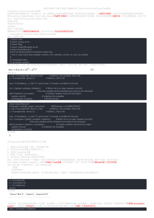
吴恩达深度学习第二课第三周编程作业_TensorFlowTutorialTensorFlow教程

吴恩达深度学习第⼆课第三周编程作业_TensorFlowTutorialTensorFlow教程TensorFlow Tutorial TensorFlow教程欢迎来到本周的编程作业。

到⽬前为⽌，您⼀直使⽤numpy来构建神经⽹络。

现在我们将引导你通过⼀个深度学习框架，它将允许你更容易地建⽴神经⽹络。

像TensorFlow, PaddlePaddle, Torch, Caffe, Keras等机器学习框架可以显著加快你机器学习的发展。

所有这些框架都有⼤量⽂档，您可以随意阅读。

在这个作业中，你将学习在TensorFlow中完成以下操作:初始化变量开始你⾃⼰的会话训练算法实现⼀个神经⽹络编程框架不仅可以缩短您的编码时间，有时还可以执⾏优化来加速您的代码。

1 - Exploring the Tensorflow Library 探索Tensorflow库⾸先，您将导⼊库:1 import math2 import numpy as np3 import h5py4 import matplotlib.pyplot as plt5 import tensorflow as tf6 from tensorflow.python.framework import ops7 from tf_utils import load_dataset, random_mini_batches, convert_to_one_hot, predict89 %matplotlib inline10 np.random.seed(1)现在您已经导⼊了库，我们将带您浏览它的不同应⽤程序。

你将从⼀个例⼦开始，我们计算⼀个训练例⼦的损失。

原代码为：y_hat = tf.constant(36, name='y_hat') # Define y_hat constant. Set to 36.y = tf.constant(39, name='y') # Define y. Set to 39loss = tf.Variable((y - y_hat)**2, name='loss') # Create a variable for the lossinit = tf.global_variables_initializer() # When init is run later (session.run(init)),# the loss variable will be initialized and ready to be computedwith tf.Session() as session: # Create a session and print the outputsession.run(init) # Initializes the variablesprint(session.run(loss)) # Prints the loss根据⽹上参考，适应tf2.0版本修改的：import tensorflow as tfpat.v1.disable_eager_execution() #保证session.run()能够正常运⾏y_hat = tf.constant(36, name='y_hat') # Define y_hat constant. Set to 36.y = tf.constant(39, name='y') # Define y. Set to 39loss = tf.Variable((y - y_hat)**2, name='loss') # Create a variable for the lossinit = pat.v1.global_variables_initializer() # When init is run later (session.run(init)),# the loss variable will be initialized and ready to be computedwith pat.v1.Session () as session: # Create a session and print the outputsession.run(init) # Initializes the variablesprint(session.run(loss))运⾏结果：在TensorFlow中编写和运⾏程序有以下步骤:1、创建Tensorflow变量（此时，尚未直接计算）2、实现Tensorflow变量之间的操作定义。

prepare_model_for_training

prepare_model_for_training 标题：为训练准备模型引言概述：在机器学习和深度学习领域，为训练准备模型是非常重要的一步。

只有经过充分准备的模型才能在训练过程中取得良好的性能。

本文将从五个大点出发，详细阐述为训练准备模型的关键步骤。

正文内容：1. 数据预处理1.1 数据清洗：去除异常值、处理缺失值和重复值。

1.2 特征工程：选择和提取与训练任务相关的特征，进行特征缩放、编码和选择。

2. 模型选择与构建2.1 模型选择：根据训练任务的特点和数据集的特征选择合适的模型，如线性回归、决策树、支持向量机等。

2.2 模型构建：根据选择的模型，确定模型的结构和参数，并进行初始化。

3. 损失函数与优化算法3.1 损失函数选择：根据训练任务的目标，选择适合的损失函数，如平方损失、交叉熵损失等。

3.2 优化算法选择：根据模型的结构和数据集的规模选择合适的优化算法，如梯度下降、Adam等。

4. 训练过程4.1 数据集划分：将数据集划分为训练集、验证集和测试集，用于模型的训练、调参和评估。

4.2 批量训练：采用批量训练的方式，每次迭代使用一小部分数据进行参数更新，提高训练效率和模型泛化能力。

4.3 参数调优：通过调整模型的超参数，如学习率、正则化参数等，优化模型的性能。

5. 模型评估与保存5.1 模型评估：使用验证集和测试集对训练好的模型进行评估，计算准确率、精确率、召回率等指标。

5.2 模型保存：将训练好的模型保存，以便后续使用和部署。

总结：在为训练准备模型的过程中，数据预处理、模型选择与构建、损失函数与优化算法、训练过程以及模型评估与保存是关键的步骤。

通过合理的准备，可以提高模型的训练效果和性能。

因此，在实际应用中，我们应该重视为训练准备模型这一步骤，以提升机器学习和深度学习模型的质量和可用性。

keyedvectors用法

keyedvectors用法Keyedvectors是一种常用于文本分类和聚类的算法，它通过将文本数据转化为向量表示，以便进行高效的数据分析和处理。

以下是Keyedvectors的基本用法和常见操作：一、基本用法Keyedvectors可以用于各种文本分类和聚类任务，例如垃圾邮件检测、情感分析、主题建模等。

使用Keyedvectors需要安装相应的库，如gensim和nltk。

安装库：```shellpipinstallgensimnltk```加载预训练模型：```pythonfromgensim.modelsimportKeyedVectorsmodel=KeyedVectors.load_word2vec_format('path/to/pretrain ed/model',binary=True)```使用KeyedVectors对象进行文本表示：```pythontext="Thisisasampletext."#输入文本vector=model[text]#将文本表示为向量```二、常见操作1.获取向量表示：使用KeyedVectors对象可以获取文本的向量表示。

可以使用模型中的任何文本进行表示。

2.相似度比较：使用KeyedVectors对象可以计算两个文本之间的相似度。

可以使用余弦相似度或欧几里得距离等度量方法进行比较。

3.聚类分析：KeyedVectors可以用于文本聚类任务，将相似的文本分组在一起。

可以使用K-means、DBSCAN等聚类算法进行聚类分析。

4.词嵌入表示：KeyedVectors可以将单词表示为向量，这些向量可以用于各种自然语言处理任务，如情感分析、命名实体识别等。

5.更新模型：如果需要更新KeyedVectors模型，可以使用gensim库中的训练方法进行训练。

例如，可以使用负采样和迭代优化方法对大规模文本数据进行训练。

文本分类和词向量训练工具fastText的参数和用法

⽂本分类和词向量训练⼯具fastText的参数和⽤法fastText的参数和⽤法fastText由Facebook开源，主要基于fasttext这篇⽂章的思路，主要⽤于两个任务：训练词向量和⽂本分类。

下载地址与document ：fasttext的主要功能：Training Supervised Classifier [supervised] Supervised Classifier Training for Text Classification. 训练分类器，就是⽂本分类，fasttext 的主营业务。

Training SkipGram Model [skipgram] Learning Word Representations/Word Vectors using skipgram technique. 训练skipgram的⽅式的词向量。

Quantization [quantize] Quantization is a process applied on a model so as to reduce the memory usage during prediction. 量化压缩，降低模型体积。

Predictions [predict] Predicting labels for a given text : Text Classification. 对于⽂本分类任务，⽤于预测类别。

Predictions with Probabilities [predict-prob] Predicting probabilities in addition to labels for a given text : Text Classification. 带有概率的预测类别。

Training of CBOW model [cbow] Learning Word Representations/Word Vectors using CBOW (Continuous Bag Of Words) technique. cbow⽅式训练词向量。

vbt训练方法

vbt训练方法VBT训练方法是一种独特而又有效的训练方式，全称为向量增量训练（Vector-based Incremental Training），是一种基于矢量化表示的深度学习模型训练方法。

VBT训练方法结合人工智能技术，通过对已有的数据进行分析，不断优化模型，从而提高模型的准确率和泛化能力。

下面我们将围绕VBT训练方法来进行分步骤的讲解。

第一步：数据预处理在VBT训练方法中，数据预处理是至关重要的一步。

数据预处理包括去除噪声、数据过滤、数据归一化等操作。

通过对数据进行预处理，可以减少噪声对模型的干扰，提高模型的准确率。

第二步：矢量化表示矢量化表示是VBT训练方法中的核心。

具体而言，就是将数据转化为向量的形式表示。

对于文本数据，可以使用Word2Vec等工具将文本转化为向量；对于图像数据，可以使用卷积神经网络将图像转化为向量；对于时间序列数据，可以使用LSTM等循环神经网络将数据转化为向量。

通过将数据转化为向量形式，可以将不同类型的数据进行统一，从而方便模型的训练。

第三步：模型训练在VBT训练方法中，模型训练是实现最终目标的关键步骤。

模型训练包括模型初始化、参数调优、损失函数选择等操作。

模型初始化是指将模型的权重和偏置初始化为随机值，以便模型能够从不同的方向开始优化。

参数调优是指根据训练过程中的反馈结果来调整模型的参数。

损失函数选择是指选择适合模型的损失函数。

在模型训练过程中，我们需要注意过拟合和欠拟合问题，以保证模型具有较高的准确率和泛化能力。

第四步：模型优化模型优化是VBT训练方法中的重要一环。

具体而言，就是通过不断地更新和调整模型的参数，使得模型的准确率和泛化能力不断提高。

常见的模型优化方法包括随机梯度下降、自适应梯度下降等。

在模型优化过程中，我们需要注意权衡准确率和效率的关系，以获得最佳的性能。

总结起来，VBT训练方法是一种基于矢量化表示的深度学习模型训练方法。

VBT训练方法通过数据预处理、矢量化表示、模型训练和模型优化等步骤来提高模型的准确率和泛化能力。

支持向量机的matlab代码

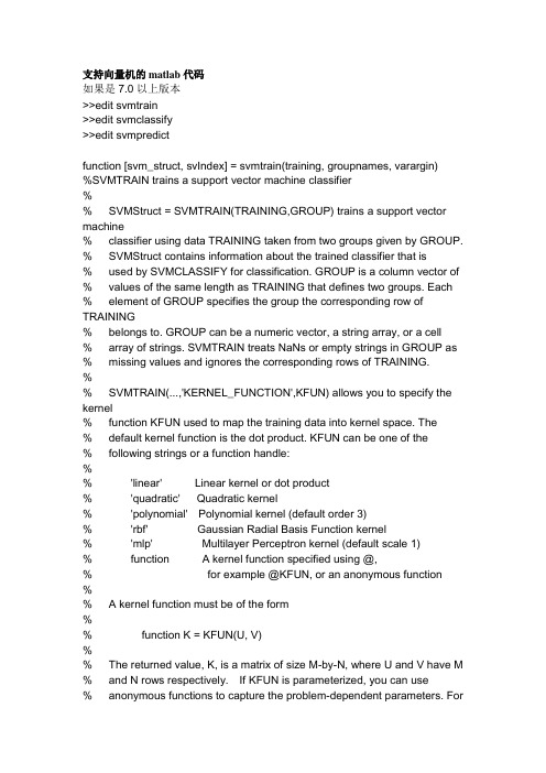
支持向量机的matlab代码如果是7.0以上版本>>edit svmtrain>>edit svmclassify>>edit svmpredictfunction [svm_struct, svIndex] = svmtrain(training, groupnames, varargin)%SVMTRAIN trains a support vector machine classifier%% SVMStruct = SVMTRAIN(TRAINING,GROUP) trains a support vector machine% classifier using data TRAINING taken from two groups given by GROUP. % SVMStruct contains information about the trained classifier that is% used by SVMCLASSIFY for classification. GROUP is a column vector of % values of the same length as TRAINING that defines two groups. Each % element of GROUP specifies the group the corresponding row of TRAINING% belongs to. GROUP can be a numeric vector, a string array, or a cell% array of strings. SVMTRAIN treats NaNs or empty strings in GROUP as % missing values and ignores the corresponding rows of TRAINING.%% SVMTRAIN(...,'KERNEL_FUNCTION',KFUN) allows you to specify the kernel% function KFUN used to map the training data into kernel space. The% default kernel function is the dot product. KFUN can be one of the% following strings or a function handle:%% 'linear' Linear kernel or dot product% 'quadratic' Quadratic kernel% 'polynomial' Polynomial kernel (default order 3)% 'rbf' Gaussian Radial Basis Function kernel% 'mlp' Multilayer Perceptron kernel (default scale 1)% function A kernel function specified using @,% for example @KFUN, or an anonymous function%% A kernel function must be of the form%% function K = KFUN(U, V)%% The returned value, K, is a matrix of size M-by-N, where U and V have M % and N rows respectively. If KFUN is parameterized, you can use% anonymous functions to capture the problem-dependent parameters. For% example, suppose that your kernel function is%% function k = kfun(u,v,p1,p2)% k = tanh(p1*(u*v')+p2);%% You can set values for p1 and p2 and then use an anonymous function: % @(u,v) kfun(u,v,p1,p2).%% SVMTRAIN(...,'POLYORDER',ORDER) allows you to specify the order of a% polynomial kernel. The default order is 3.%% SVMTRAIN(...,'MLP_PARAMS',[P1 P2]) allows you to specify the% parameters of the Multilayer Perceptron (mlp) kernel. The mlp kernel% requires two parameters, P1 and P2, where K = tanh(P1*U*V' + P2) and P1% > 0 and P2 < 0. Default values are P1 = 1 and P2 = -1.%% SVMTRAIN(...,'METHOD',METHOD) allows you to specify the method used% to find the separating hyperplane. Options are%% 'QP' Use quadratic programming (requires the Optimization Toolbox) % 'LS' Use least-squares method%% If you have the Optimization Toolbox, then the QP method is the default % method. If not, the only available method is LS.%% SVMTRAIN(...,'QUADPROG_OPTS',OPTIONS) allows you to pass an OPTIONS% structure created using OPTIMSET to the QUADPROG function when using% the 'QP' method. See help optimset for more details.%% SVMTRAIN(...,'SHOWPLOT',true), when used with two-dimensional data,% creates a plot of the grouped data and plots the separating line for% the classifier.%% Example:% % Load the data and select features for classification% load fisheriris% data = [meas(:,1), meas(:,2)];% % Extract the Setosa class% groups = ismember(species,'setosa');% % Randomly select training and test sets% [train, test] = crossvalind('holdOut',groups);% cp = classperf(groups);% % Use a linear support vector machine classifier% svmStruct = svmtrain(data(train,:),groups(train),'showplot',true); % classes = svmclassify(svmStruct,data(test,:),'showplot',true);% % See how well the classifier performed% classperf(cp,classes,test);% cp.CorrectRate%% See also CLASSIFY, KNNCLASSIFY, QUADPROG, SVMCLASSIFY.% Copyright 2004 The MathWorks, Inc.% $Revision: 1.1.12.1 $ $Date: 2004/12/24 20:43:35 $% References:% [1] Kecman, V, Learning and Soft Computing,% MIT Press, Cambridge, MA. 2001.% [2] Suykens, J.A.K., Van Gestel, T., De Brabanter, J., De Moor, B., % Vandewalle, J., Least Squares Support Vector Machines,% World Scientific, Singapore, 2002.% [3] Scholkopf, B., Smola, A.J., Learning with Kernels,% MIT Press, Cambridge, MA. 2002.%% SVMTRAIN(...,'KFUNARGS',ARGS) allows you to pass additional% arguments to kernel functions.% set defaultsplotflag = false;qp_opts = [];kfunargs = {};setPoly = false; usePoly = false;setMLP = false; useMLP = false;if ~isempty(which('quadprog'))useQuadprog = true;elseuseQuadprog = false;end% set default kernel functionkfun = @linear_kernel;% check inputsif nargin < 2error(nargchk(2,Inf,nargin))endnumoptargs = nargin -2;optargs = varargin;% grp2idx sorts a numeric grouping var ascending, and a string grouping% var by order of first occurrence[g,groupString] = grp2idx(groupnames);% check group is a vector -- though char input is special...if ~isvector(groupnames) && ~ischar(groupnames)error('Bioinfo:svmtrain:GroupNotVector',...'Group must be a vector.');end% make sure that the data is correctly oriented.if size(groupnames,1) == 1groupnames = groupnames';end% make sure data is the right sizen = length(groupnames);if size(training,1) ~= nif size(training,2) == ntraining = training';elseerror('Bioinfo:svmtrain:DataGroupSizeMismatch',...'GROUP and TRAINING must have the same number of rows.') endend% NaNs are treated as unknown classes and are removed from the training % datanans = find(isnan(g));if length(nans) > 0training(nans,:) = [];g(nans) = [];endngroups = length(groupString);if ngroups > 2error('Bioinfo:svmtrain:TooManyGroups',...'SVMTRAIN only supports classification into two groups.\nGROUP contains %d different groups.',ngroups)end% convert to 1, -1.g = 1 - (2* (g-1));% handle optional argumentsif numoptargs >= 1if rem(numoptargs,2)== 1error('Bioinfo:svmtrain:IncorrectNumberOfArguments',...'Incorrect number of arguments to %s.',mfilename);endokargs ={'kernel_function','method','showplot','kfunargs','quadprog_opts','polyorder','ml p_params'};for j=1:2:numoptargspname = optargs{j};pval = optargs{j+1};k = strmatch(lower(pname), okargs);%#okif isempty(k)error('Bioinfo:svmtrain:UnknownParameterName',...'Unknown parameter name: %s.',pname);elseif length(k)>1error('Bioinfo:svmtrain:AmbiguousParameterName',...'Ambiguous parameter name: %s.',pname);elseswitch(k)case 1 % kernel_functionif ischar(pval)okfuns = {'linear','quadratic',...'radial','rbf','polynomial','mlp'};funNum = strmatch(lower(pval), okfuns);%#okif isempty(funNum)funNum = 0;endswitch funNum %maybe make this less strict in the futurecase 1kfun = @linear_kernel;case 2kfun = @quadratic_kernel;case {3,4}kfun = @rbf_kernel;case 5kfun = @poly_kernel;usePoly = true;case 6kfun = @mlp_kernel;useMLP = true;otherwiseerror('Bioinfo:svmtrain:UnknownKernelFunction',...'Unknown Kernel Function %s.',kfun);endelseif isa (pval, 'function_handle')kfun = pval;elseerror('Bioinfo:svmtrain:BadKernelFunction',...'The kernel function input does not appear to be a function handle\nor valid function name.')endcase 2 % methodif strncmpi(pval,'qp',2)useQuadprog = true;if isempty(which('quadprog'))warning('Bioinfo:svmtrain:NoOptim',...'The Optimization Toolbox is required to use the quadratic programming method.')useQuadprog = false;endelseif strncmpi(pval,'ls',2)useQuadprog = false;elseerror('Bioinfo:svmtrain:UnknownMethod',...'Unknown method option %s. Valid methods are ''QP'' and ''LS''',pval);endcase 3 % displayif pval ~= 0if size(training,2) == 2plotflag = true;elsewarning('Bioinfo:svmtrain:OnlyPlot2D',...'The display option can only plot 2D training data.')endendcase 4 % kfunargsif iscell(pval)kfunargs = pval;elsekfunargs = {pval};endcase 5 % quadprog_optsif isstruct(pval)qp_opts = pval;elseif iscell(pval)qp_opts = optimset(pval{:});elseerror('Bioinfo:svmtrain:BadQuadprogOpts',...'QUADPROG_OPTS must be an opts structure.');endcase 6 % polyorderif ~isscalar(pval) || ~isnumeric(pval)error('Bioinfo:svmtrain:BadPolyOrder',...'POLYORDER must be a scalar value.');endif pval ~=floor(pval) || pval < 1error('Bioinfo:svmtrain:PolyOrderNotInt',...'The order of the polynomial kernel must be a positive integer.')endkfunargs = {pval};setPoly = true;case 7 % mlpparamsif numel(pval)~=2error('Bioinfo:svmtrain:BadMLPParams',...'MLP_PARAMS must be a two element array.');endif ~isscalar(pval(1)) || ~isscalar(pval(2))error('Bioinfo:svmtrain:MLPParamsNotScalar',...'The parameters of the multi-layer perceptron kernel must be scalar.');endkfunargs = {pval(1),pval(2)};setMLP = true;endendendendif setPoly && ~usePolywarning('Bioinfo:svmtrain:PolyOrderNotPolyKernel',...'You specified a polynomial order but not a polynomial kernel');endif setMLP && ~useMLPwarning('Bioinfo:svmtrain:MLPParamNotMLPKernel',...'You specified MLP parameters but not an MLP kernel');end% plot the data if requestedif plotflag[hAxis,hLines] = svmplotdata(training,g);legend(hLines,cellstr(groupString));end% calculate kernel functiontrykx = feval(kfun,training,training,kfunargs{:});% ensure function is symmetrickx = (kx+kx')/2;catcherror('Bioinfo:svmtrain:UnknownKernelFunction',...'Error calculating the kernel function:\n%s\n', lasterr);end% create Hessian% add small constant eye to force stabilityH =((g*g').*kx) + sqrt(eps(class(training)))*eye(n);if useQuadprog% The large scale solver cannot handle this type of problem, so turn it % off.qp_opts = optimset(qp_opts,'LargeScale','Off');% X=QUADPROG(H,f,A,b,Aeq,beq,LB,UB,X0,opts)alpha = quadprog(H,-ones(n,1),[],[],...g',0,zeros(n,1),inf *ones(n,1),zeros(n,1),qp_opts);% The support vectors are the non-zeros of alphasvIndex = find(alpha > sqrt(eps));sv = training(svIndex,:);% calculate the parameters of the separating line from the support% vectors.alphaHat = g(svIndex).*alpha(svIndex);% Calculate the bias by applying the indicator function to the support% vector with largest alpha.[maxAlpha,maxPos] = max(alpha); %#okbias = g(maxPos) - sum(alphaHat.*kx(svIndex,maxPos));% an alternative method is to average the values over all support vectors % bias = mean(g(sv)' - sum(alphaHat(:,ones(1,numSVs)).*kx(sv,sv)));% An alternative way to calculate support vectors is to look for zeros of % the Lagrangians (fifth output from QUADPROG).%% [alpha,fval,output,exitflag,t] = quadprog(H,-ones(n,1),[],[],...% g',0,zeros(n,1),inf *ones(n,1),zeros(n,1),opts);%% sv = t.lower < sqrt(eps) & t.upper < sqrt(eps);else % Least-Squares% now build up compound matrix for solverA = [0 g';g,H];b = [0;ones(size(g))];x = A\b;% calculate the parameters of the separating line from the support% vectors.sv = training;bias = x(1);alphaHat = g.*x(2:end);endsvm_struct.SupportVectors = sv;svm_struct.Alpha = alphaHat;svm_struct.Bias = bias;svm_struct.KernelFunction = kfun;svm_struct.KernelFunctionArgs = kfunargs;svm_struct.GroupNames = groupnames;svm_struct.FigureHandles = [];if plotflaghSV = svmplotsvs(hAxis,svm_struct);svm_struct.FigureHandles = {hAxis,hLines,hSV}; end41|评论(6)。

DBoW2库介绍

DBoW2库介绍DBoW2库是University of Zaragoza⾥的Lopez等⼈开发的开源软件库。

由于在SLAM回环检测上的优异表现（特别是ORB-SLAM2），DBoW2库受到了⼴⼤SLAM爱好者的关注。

本⽂希望通过深⼊解析DBoW2库及相关的DLoopDetector库，为读者后续使⽤这两个库提供参考。

git地址：论⽂：Bags of Binary Words for Fast Place Recognition in Image SequencesDBoW2库介绍词袋模型BoW（Bag of Words，词袋模型），是⾃然语⾔处理领域经常使⽤的⼀个概念。

以⽂本为例，⼀篇⽂章可能有⼀万个词，其中可能只有500个不同的单词，每个词出现的次数各不相同。

词袋就像⼀个个袋⼦，每个袋⼦⾥装着同样的词。

这构成了⼀种⽂本的表⽰⽅式。

这种表⽰⽅式不考虑⽂法以及词的顺序。

在计算机视觉领域，图像通常以特征点及其特征描述来表达。

如果把特征描述看做单词，那么就能构建出相应的词袋模型。

这就是本⽂介绍的DBoW2库所做的⼯作。

利⽤DBoW2库，图像可以⽅便地转化为⼀个低维的向量表⽰。

⽐较两个图像的相似度也就转化为⽐较两个向量的相似度。

它本质上是⼀个信息压缩的过程。

视觉词典词袋模型利⽤视觉词典（vocabulary）来把图像转化为向量。

视觉词典有多种组织⽅式，对应于不同的搜索复杂度。

DBoW2库采⽤树状结构存储词袋，搜索复杂度⼀般在log(N)，有点像决策树。

词典的⽣成过程如下图。

这棵树⾥⾯总共有1+K+\cdots+K^L=(k^{L+1}-1)/(K-1)个节点。

所有叶节点在L层形成W=K^L类，每⼀类⽤该类中所有特征的平均特征（meanValue）作为代表，称为单词（word）。

每个叶节点被赋予⼀个权重。

作者提供了TF、IDF、BINARY、TF-IDF等权重作为备选，默认为TF-IDF。

TF-IDF的主要思想是：如果某个词或短语在⼀篇⽂章中出现的频率TF⾼，并且在其他⽂章中很少出现，则认为此词或者短语具有很好的类别区分能⼒，适合⽤来分类。

利用PythonNumpy从零开始步步为营计算Word2Vec词向量

利⽤PythonNumpy从零开始步步为营计算Word2Vec词向量利⽤Python Numpy从零开始步步为营计算Word2Vec词向量⽜伯⾬词向量建模是⾃然语⾔处理当中的重要基础步骤。

有了⽤向量表⽰的词汇，计算机就可以更好地处理⽂本数据了。

2013年，提出的Word2Vec是⼀个⾥程碑式的词向量建模⽅法。

最近看到⼀篇的关于徒⼿计算Word2Vec的博⽂，作者利⽤表格软件表现这种模型训练过程中的矩阵和向量的变化，这对理解这种模型的原理⼤有裨益。

另⼀篇GeeksforGeeks 上题为的⽂章对这⼀模型也有⽐较详细的说明。

本⽂是受此启发的产物，表格设计风格和部分代码有参考，旨在动⼿利⽤Python⾥的Numpy⼀步步地从零构建Word2Vec词向量。

1. CBOW模型和Skip-gram模型Mikolov等⼈2013年的论⽂提出了两种模型，它们分别叫Continuous Bag of Words（CBOW）和Continuous Skip-gram，图⽰如下：这两种模型都是预测模型，不过CBOW是已知某个词（中⼼词）周围的上下⽂，来预测这个词本⾝最有可能是什么，⽽Skip-gram则是已知⼀个词（中⼼词），来预测这个词周围最有可能是哪些词作为它的上下⽂。

这两种模型看上去相似，有相互对称的感觉，在具体的操作中也有⼀些区别。

Mikolov 2013年的原⽂第4.3节对这两种模型进⾏了⽐较：1. 在模型训练时间⽅⾯，Skip-gram所需的时间基本上是CBOW的3倍。

这⼀件⽐较符合我们的直观感受：已知上下⽂去预测其中的某⼀个词，是⽐只知道⼀个词去预测上下⽂要简单很多的。

2. 在模型表现⽅⾯，Skip-gram在语义上的表现要优于CBOW，⽽CBOW则在句法上稍微更胜⼀筹。

具体说来，如果我们⽤英⽂⽂本举例⼦，在单词相似性的任务⾥，Skip-gram更倾向于将"dog"和"cat"这类语义相近的单词视为相似词，⽽CBOW则可能会认为"dog"和其复数形式"dogs"更接近。