uppaal-tutorial
UPPAAL建模工具教程

Uppaal4.0:Small Tutorial∗16November20091IntroductionThis document is intended to be used by newcomers to Uppaal and verification.Students or engineers with little background in formal methods should be able to use Uppaal for practical purposes after this tutorial.Section2describes Uppaal and Section3is the tutorial itself.2UppaalUppaal is a tool box for validation(via graphical simulation)and verification(via automatic model-checking)of real-time systems.It consists of two main parts:a graphical user interface and a model-checker engine.The user interface is implemented in Java and is executed on the users work station.Version4.0of Uppaal requires that the Java Runtime Environment5or higher is installed on the computer.The engine part is by default executed on the same computer as the user interface,but can also run on a more powerful server.The idea is to model a system using timed automata,simulate it and then verify properties on it.Timed automata arefinite state machines with time(clocks).A system consists of a network of processes that are composed of locations.Transitions between these locations define how the system behaves.The simulation step consists of running the system interactively to check that it works as intended.Then we can ask the verifier to check reachability properties,i.e.,if a certain state is reachable or not.This is called model-checking and it is basically an exhaustive search that covers all possible dynamic behaviours of the system.More precisely,the engine uses on-the-fly verification combined with a symbolic technique re-ducing the verification problem to that of solving simple constraint systems[YPD94,LPY95].The verifier checks for simple invariants and reachability properties for efficiency reasons.Other prop-erties may be checked by using testing automata[JLS96]or the decorated system with debugging information[LPY97].3Learning UppaalUppaal is based on timed automata,that isfinite state machine with clocks.The clocks are the way to handle time in Uppaal.Time is continuous and the clocks measure time progress.It is allowed to test the value of a clock or to reset it.Time will progress globally at the same pace for the whole system.A system in Uppaal is composed of concurrent processes,each of them modeled as an automa-ton.The automaton has a set of locations.Transitions are used to change location.To control when to take a transition(to“fire”it),it is possible to have a guard and a synchronization.A guard is a condition on the variables and the clocks saying when the transition is enabled.The synchronization mechanism in Uppaal is a hand-shaking synchronization:two processes take a ∗This description covers version4.0.7transition at the same time,one will have an a!and the other an a?,with a being the synchro-nization channel.When taking a transition,two actions are possible:assignment of variables or reset of clocks.The following examples will make you familiar with this short description.3.1OverviewThe Uppaal main window(Figure1)has two main parts:the menu and the tabs.Figure1:Overview of Uppaal.The menu is described in the integrated help,accessible through the help menu.The help further describes the used syntax and the GUI in detail,so this tutorial will focus on how to use the tool.The three tabs give access to the three components of Uppaal that are the editor,the simulator and the verifier.Figure1shows the editor view.The idea is to define templates(like in C++)for processes that are instantiated to have a complete system.The motivation for the templates is that system often have several processes that are very alike.The control structure(i.e.,the locations and edges) is the same,only some constant or variable is different.Therefore templates can have symbolic variables and constants as parameters.A template may also have have local variables and clocks.When you start Uppaal,there is one location pre-created in the drawing area.It is the initial location of the automaton,so it has an additional circle inside.To add a second location,click on the“Add Location”button in the tool bar(tool tips will help you)and then click in the drawing area,a bit next to the initial e the“Selection Tool”to give them the names start and end.Then choose the Add Edge button,click on the start location and on the end location. You have yourfirst automaton ready,as depicted in Figure2.There is another important detail in the editor which you should know about.On the bottom of the screen,there is a bar which you can“drag up”.This will open a table with rows Position and Description which is most likely empty at that ter,it will contain very useful information about syntactical compile errors that your model ing this will make it much easier tofind andfix them.Figure2:Yourfirst automaton.Now,click on the Simulator tab to start the simulator,click on the yes button that will pop up and you are ready to run yourfirst system.Figure3:A snapshot of the graphical simulator.Figure3shows the simulator view.On the left you willfind the control part where you can choose the transitions(upper part)and work on an existing trace(lower part).In the middle are the variables and on the right you see the system itself.Below the system,you will see what happens in which process.To simulate our trivial system pick one of the enabled transitions in the list in the upper left part of the screen.Of course there is only one transition in our example.Click Next.The process view to the right will change(the red dot indicating the current location will move)and the simulation trace will grow.You will note that more transitions are actually not possible,so the system is deadlocked.We have now simulated our system and will proceed with verification.Click on the Verifier tab.The verifier view as in Figure4is displayed.The upper section allows you to specify queries to the system.The lower part logs the communication with the model-checking engine.Enter the text E<>Process.end in the Queryfield below the Overview.This is the UppaalFigure4:A snapshot of the verifier view.notation for the temporal logic formula∃⋄P rocess.end and should be understood as“it is possible to reach the location end in automaton Process”.Click Check to let the engine verify this.The bullet in the overview will turn green indicating that he property indeed is satisfied.The goal of the rest of this document is to explore some key points of Uppaal through examples.3.2Mutual Exclusion AlgorithmWe will study now the known Petterson’s mutual exclusion algorithm to see how we can derive a model as an automaton from a program/algorithm and check properties related to it.The algorithm for two processes is as follows in C:Process1Process2req1=1;req2=1;turn=2;turn=1;while(turn!=1&&req2!=0);while(turn!=2&&req1!=0);//critical section://critical section:job1();job2();req1=0;req2=0;You will construct the corresponding automata.Notice that the protocol is symmetric,so we may use a template of Uppaal to simplify the model.First reset the system(New system)to clear the“Hello World”example.Rename the default template P to mutex.We will abstract the actual work in the critical section since it has no interest here.The protocol has four states that come directly from the described algorithm,similar to goto labels.Using these,both processes can be written as follows:Process1idle:req1=1;want:turn=2;wait:while(turn!=1&&req2!=0); CS://critical sectionjob1();req1=0;//and return to idle Process2idle:req2=1;want:turn=1;wait:while(turn!=2&&req1!=0); CS://critical sectionjob2();req2=0;//and return to idleAs automata,the processes will look as depicted in Figure5.req2 == 0req1 == 0 Figure5:Mutex automataThe blue expressions are assignments to variables,that are executed when the correspond-ing transition is taken.The green expressions are guards that have to be true in order for the corresponding transition to be enabled.You may notice that the two automata look very alike.The only difference are certain values and variable names.In order to save work,we will define just one template automaton,and then instantiate this template twice.The template may look as in Figure6.Note that we replace the variables req1and req2with placeholders req self and req other which we will instantiate later.The new variable me will indicate to the instance,which process it represents.req_other == 0Figure6:Mutex templateIn order to create a template,youfirst draw the automaton from Figure5as before.Let’scall this template“mutex”,which you specify in the Name:field right above the drawing area.In addition,you must specify the template parameters me,req self and req other.You do this by writing them in the Parameters:field right next to the Name:field.Write the following:const int[1,2]me,int[0,1]&req_self,int[0,1]&req_otherThis means that you define three variables for instantiation of type integer,bounded to two values each.Thefirst one,me,is a constant,and the other two have to be variables with boolean values(0or1).As you can guess now from your drawing,two instances of the type P1=mutex(1,req1, req2);and P2=mutex(2,req2,req1);will do the job.Examine how the expression(like C syntax)turn:=(me==1?2:1)will evaluate.To create the instances open the System declarations label in the Project tree and type the declarations above(replacing the default line that instantiates the default template).In addition,specify that the system now consists of P1and P2by writing them behind the keyword system,comma-separated.The System declarations contain now://Place template instantiations here.P1=mutex(1,req1,req2);P2=mutex(2,req2,req1);//List one or more processes to be composed into a system.system P1,P2;Something is still missing:the variables also have to be declared.Click on the Declarations label and declare:int[0,1]req1,req2;and int[1,2]turn;Now you have defined your template,instantiated it twice,used the instantiations in the system and declared proper variables.As you may notice,the variables declared are global.This is used for turn that is shared.The scope of the name declaration are localfirst and then global.Before we go on,do a syntax check(Tools menu or press F7)and have a look in the list that you can drag up below the drawing area.It should be empty,otherwisefix the reported issues.Now,click on the Simulator tab and examine how the two automata were instantiated.Look particularly at the names of the two automata that are symmetric.You can simulate your system by choosing interactively the transitions.Try to reach the critical section in both processes at the same time...well you cannot,that’s the point of the protocol.But using simulation,we can’t be sure about this.A better idea is to use the verifier.Click on the Verifier tab,click on the Insert button,click in the Query text area and write the mutual exclusion property:A[]not(P1.CS and P2.CS).Press the Check button and you are done.There should be a green button lighted on,which means that the property was verified. If the button were red it would mean that the property was not verified.The property A[]is a safety property:you check that not(P1.CS and P2.CS)is always true.Another type of property, the E<>may be used for reachability properties.For example insert a new property E<>P1.CS, that checks if process P1may reach the critical section.If the system was not correct Uppaal can return an diagnostic trace.First change the model so it is faulty.E.g.change the guard req other==0to req other==1.Then go to the Options menu and activate one of the Diagnostic Trace options;select the mutual exclusion property, then press the Check button.Now this property should not be satisfied.You can now return to the simulator and go through the found trace.Choose thefirst entry in the trace and then press Replay for this.You have now modeled,simulated and verified a simple mutual exclusion protocol.In the demo folder in the distribution directory there are a few other simple examples.For example the file fischer.xml contains another mutual exclusion protocol,together with some example queries in fischer.q.3.3Time in UppaalThis sub-section intends to explain intuitively the concept of time in Uppaal .The time model in Uppaal is continuous time.Technically,it is implemented as regions and the states are thus symbolic,which means that at a state we do not have any concrete value for the time,but rather differences [AD94].To grasp how the time is handled in Uppaal we will study a simple example.We will use an observer to show the differences.Normally,an observer is an add-on automaton in charge of detecting events without perturbing the observed system.In our case the reset of the clock (x :=0)is delegated to the observer to make it work.Note that by doing this,the original behaviour of the system –with the clock reset directly on the transition loop to itself –is not changed.Figure 7shows the first model with its observer.Time is used through clocks .In the example,x is a clock declared as clock x;in the global Declarations section.A channel reset is used for synchronization with the observer,which is also declared (as chan reset )in the Declarations section.The channel synchronization is a hand-shaking between reset!and reset?in our example.So in this example the clock may be reset after 2time units.The observer detects this and actually performs the reset.x >= 2reset!reset?Figure 7:First example with the automata P1and Obs observer.Draw the model,name the automata P1and Obs ,define them in the system.A new template is created with Insert Template in the Edit menu.(You can just write the template names directly in the system statement,Uppaal will automatically instantiate them for you.)Notice that the state taken of the observer is of type committed .If you simulate the system you will not see much.To train to interpret what you see we will use queries and modify the system progressively.The expected behaviour of our system is depicted in Figure 8.246824"time"c l o c k xFigure 8:Time behaviour of the first example:this is one possible run.Try these properties to exhibit this behaviour:•A[]Obs.taken imply x>=2:all fall-down of the clock value (see curve)are above 2.This query means:for all states,being in the location Obs.taken implies that x>=2.•E<>Obs.idle and x>3:this is for the waiting period,you can try values like 30000and you will get the same result.This question means:is it possible to reach a state where Obs is in the location idle and x>3.Add now an invariant to the loop location as shown in Figure 9.x <= 3x >= 2reset!246824"time"c l o c k xFigure 9:Adding an invariant:the new behaviour.The invariant is a progress condition :the system is not allowed to stay in the state more than 3time units (more precisely:only as long as the clock x is no larger than 3),so the transition has to be taken and the clock reset in our example.To see the difference,try the properties:•A[]Obs.taken imply (x>=2and x<=3)to show that the transition is taken when x is in the interval [2,3].•E<>Obs.idle and x>2:it is possible to take the transition with x in the interval (2,3].•A[]Obs.idle imply x<=3:to show that the upper bound is respected.The former property E<>Obs.idle and x>3no longer holds.Now,remove the invariant and change the guard to x >=2and x <=3.You may think that it is the same as before –but it is not!The system has no progress condition anymore,just a new condition on the guard now.Figure 10shows the newsystem.x >=2 and x <= 3reset!246824"time"c l o c k xFigure 10:No invariant and a new guard:the new behaviour.As you can see the system may take the same transitions as before,but there is now a deadlock:the system may be stuck if it does not take the transition after 3time units.Retry the same properties,the last one does not hold now.Actually you can see the deadlock with the following property:A[]x>3imply not Obs.taken ,that is after 3time units the transition can not be taken any more.3.4Urgent/Committed LocationsWe will now look at the different kinds of locations of Uppaal.You already saw the type committed in the previous example.There are three different types of locations in Uppaal: Normal locations with or without invariants(like x<=3above),Urgent locations andCommitted locations as used in the Obs automaton.Draw the automata depicted in Figure11and name them P0,P1and P2.Define the clocks x locally for each automaton,in order to try this feature:open the sub-tree of their templates in the Project tree.There you will see a Declarations label under the template in question.Click on it and define clock x;.Repeat for the other two automata.Figure11:Automata with normal,urgent and committed states.The location marked“U”is urgent and the one marked“C”is committed.Try them in the simulator and notice that when in the committed state,the only possible transition is always the one going out of the committed state.The committed state has to be left immediately.To see the difference between normal and urgent state,go to the verifier and try the properties:•E<>P0.S1and P0.x>0:it is possible to wait in S1of P0.•A[]P1.S1imply P1.x==0:it is not possible to wait in S1of P1.Time may not pass in an urgent state,but interleavings with normal states are allowed as you can see in the simulator.Thus,urgent locations are“less strict”variants than committed ones.3.5Verifying propertiesIn the examples above we have used the verifier several times.We will now give a more complete treatment of the language that the verifier understands.In summary,the queries available in the verifier are:•E<>p:there exists a path where p eventually holds.•A[]p:for all paths p always holds.•E[]p:there exists a path where p always holds.•A<>p:for all paths p will eventually hold.•p-->q:whenever p holds q will eventually hold.where p and q are state formulas like for example(P1.cs and x<3).The full grammar of the query language is available in the on-line help.Note the useful special form A[]not deadlock that checks for deadlocks.3.6Some Modeling TricksUppaal offers urgent channels(defined using urgent chan)that are synchronization that must be taken when the transition is enabled,without delay.Clock conditions on these transitions are not allowed.It is possible to encode“urgent transitions”with a guard on a variable,i.e.busy wait on a variable,by using urgent e a dummy process with one state looping with one transition read!.The urgent transition will be x>0read?for example.There is no value passing through the channels but this is easily encoded by shared variable: define globally a variable x,and use it for reading and writing.Notice that it is not clean to do read!x:=3;and read?y:=x;but it is better to use a committed location in between:First the read?transition into the committed location,then the transition setting y:=x;.Since Uppaal4,broadcast communication is also possible:The intuition is that an edge with synchronisation label e!emits a broadcast on the channel e and that any enabled edge with synchronisation label e?will synchronise with the emitting process.More details are given in the online help.Arrays of integers may be useful,declare them as int a[3];to have an array indexable from 0to2.The index can be another variable i typically int[0,2]i;to be clean.To keep a model manageable,one has to pay attention to some points:•The number of clocks has an important impact on the complexity,i.e.,on the verification time,since it highly influences the state space.•The use of committed locations can reduce significantly the state space,but one has to be careful with this feature because it can possibly take away relevant states.•The number of variables plays an important role as well and more importantly their range.One should be careful that the integer will not use all the values from-32000to32000for example.In particular avoid unbounded loops on integers since the values will then span over the full range.References[YPD94]Wang Yi,Paul Pettersson,and Mats Daniels.Automatic Verification of Real-Time Com-municating Systems By Constraint-Solving.In Proc.of the7th International Conference on Formal Description Techniques,1994.[LPY95]Kim rsen,Paul Pettersson,and Wang Yi.Model-Checking for Real-Time Sys-tems.In Proc.of Fundamentals of Computation Theory,volume965of Lecture Notes in Computer Science,pages62–88,August1995.[JLS96]H.E.Jensen,rsen,and A.Skou.Modelling and Analysis of a Collision Avoidance Protocol Using SPIN and Uppaal.In Proc.of2nd International Workshop on the SPIN Verification System,pages1–20,August1996.[LPY97]Magnus Lindahl,Paul Pettersson,and Wang Yi.Formal Design and Analysis of a Gear-Box Controller:an Industrial Case Study using Uppaal.In preparation,1997.[AD94]R.Alur and D.Dill.A Theory for Timed Automata In Theoretical Computer Science, volume125,pages183–235,1994.Version historyMarch2001First version by Alexandre David.28Apr2001Corrections by Alexandre David.Bug in a requirement,added:chan declaration, bug in declarations:int[0,1]req1,req2,turn;turn is int,not int[0,1]!17Dec2001Updates by Alexandre David.Added how to mark initial states(because the new UPPAAL does not make thefirst state initial by default anymore).160ct2002Updates by Tobias Amnell.Changed screen-shoots to recent version(3.2.11),added verification walk-through in start-end example,added section on query language plus text updates on several places.16Nov2009Updates by Martin Stigge.Adapted document to version4.0.7of Uppaal(syntax and screenshots).More detailed version of the mutex example to decrease confusion.A bunch of minorfixes and clarifications,thanks to Pontus Ekberg.11。
unscrambler PLS1建模 自己总结的详细步骤
By liao2013.1.22Unscrambler9.7 PLS1建模帮助自带例题tutor_a每一步超详细步骤,自己总结加翻译,帮助大家学习。
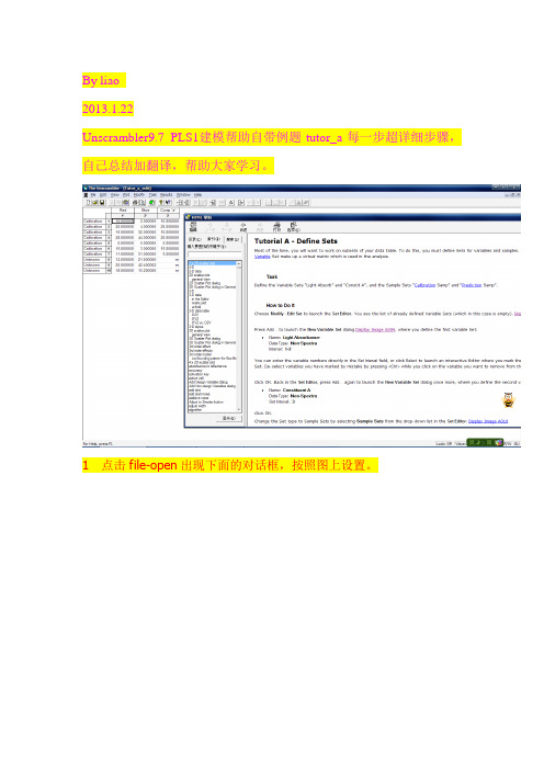
1 点击file-open出现下面的对话框,按照图上设置。
选择tutor_a数据文件,出现下图即为原始数据,导入成功。
2 基本设置,方便建模,分为校正集(calibration)、验证集(validation)点击modify-edit sets-variable sets-add再add:modify-edit sets-samples sets-add3 单变量模型的建立(1)先画个二维散点图长按着Ctrl点击Red和Comp “a”。
点击Plot - 2D Scatter ,选择“Calibration Samples”。
点击OK后:趋势线的绘制:View - Trend Lines - Regression Line/Target Line (2)点击Esc键,放弃选择。
点击Task - Regression点击OK点击OK 点击View(3)模型系数图点击Plot - Regression Coefficients点击Edit - Options-BarsConcentration of “a”= 1E-06 + 1.04 * Red– 0.208 * Blue 保存模型,file-save as-tutorial A4 模型预测(1)回到数据表data-Tutor_a。
点击Task - Predict保存为“Tutorial A Prediction 1”(2)模型系数点击Results - Regression选择Tutorial A.选中右下角的第四幅图,点击Plot - Predicted vs Measured 如下图模型效果很好。
View - Trend Lines 绘制目标曲线View - Plot Statistics 统计值5 用正确的验证方法重新校正模型回到数据表data-Tutor_a。
tutorial_1 soluation

Hardware Macstuff Winstuff 200 100
Software 1000 1500
In this economy the firm whose opportunity cost of producing a good is lowest is said to have a comparative advantage (CA) in producing that good. The firm with an absolute advantage (AA) in producing a good produces that good with the least amount of resources. Opportunity cost of producing 1 unit of: Hardware Macstuff Winstuff 5 units of software 15 units of software Software 1/5 units of hardware 1/15 units of hardware
Question 3 There are two firms: Macstuff and Winstuff. Each firm can produce either software or hardware using their resources. With one unit of its own resources Macstuff can produce 200 units of hardware or 1000 units of software. With one unit of its own resources Winstuff can produce 100 units of hardware or 1500 units of software. Each firm has 10 units of resources to allocate to the production of software and hardware. Suppose Macstuff and Winstuff agree to specialise their production according to their comparative advantage in producing software and hardware, and to then exchange with each other. Identify the bounds on the terms at which they would agree to trade software for hardware? Express your answer in terms of the amount of hardware that would be ‘paid’ for software. Explain your answer.
psacal教程

第一章简单程序无论做任何事情,都要有一定的方式方法与处理步骤。
计算机程序设计比日常生活中的事务处理更具有严谨性、规范性、可行性。
为了使计算机有效地解决某些问题,须将处理步骤编排好,用计算机语言组成“序列”,让计算机自动识别并执行这个用计算机语言组成的“序列”,完成预定的任务。
将处理问题的步骤编排好,用计算机语言组成序列,也就是常说的编写程序。
在Pascal语言中,执行每条语句都是由计算机完成相应的操作。
编写Pascal程序,是利用Pascal 语句的功能来实现和达到预定的处理要求。
“千里之行,始于足下”,我们从简单程序学起,逐步了解和掌握怎样编写程序。
第一节Pascal 程序结构和基本语句在未系统学习Pascal语言之前,暂且绕过那些繁琐的语法规则细节,通过下面的简单例题,可以速成掌握Pascal程序的基本组成和基本语句的用法,让初学者直接模仿学习编简单程序。
[例1.1]编程在屏幕上显示“Hello World!”。
Pascal程序:Program ex11;BeginWriteln(‘Hello World!’);ReadLn;End.这个简单样例程序,希望大家的程序设计学习能有一个良好的开端。
程序中的Writeln是一个输出语句,它能命令计算机在屏幕上输出相应的内容,而紧跟Writeln语句后是一对圆括号,其中用单引号引起的部分将被原原本本地显示出来。
[例1.2]已知一辆自行车的售价是300元,请编程计算a辆自行车的总价是多少?解:若总售价用m来表示,则这个问题可分为以下几步处理:= 1 \* GB3 ①从键盘输入自行车的数目a;= 2 \* GB3 ②用公式m=300*a 计算总售价;= 3 \* GB3 ③输出计算结果。
Pascal程序:Program Ex12; {程序首部} Var a,m : integer; {说明部分} Begin{语句部分}Write(‘a=’);ReadLn(a);{输入自行车数目}M := 300*a; {计算总售价}Writeln(‘M=’,m); {输出总售价}ReadLn;{等待输入回车键}End.此题程序结构完整,从中可看出一个Pascal 程序由三部分组成:(1)程序首部由保留字Program开头,后面跟一个程序名(如:Exl1);其格式为:Program 程序名;程序名由用户自己取,它的第一个字符必须是英文字母,其后的字符只能是字母或数字和下划线组成,程序名中不能出现运算符、标点符和空格。
PAUP 4.0的中文快速使用手册(Quick Start Tutorial)
PAUP 4.0的中文快速使用手册(Quick Start Tutorial)下面的指南手册对PAUP4.O 的基本用法提供了一个非常简洁的概述。
这个指南将通过分析例子数据文件中的一个例子来一步一步教会你. 这个例子可以在你提供给你的盘里,也可以在/data/primate-mtDNA-interleaved.nex上下载.这个指南为那些以前没有用过PAUP 经历的人设计,如果你已经很熟悉PAUP,那么你可以跳过这个指南,我们假定用户已对系统发育术语和特别的计算机操作系统很熟悉.如对DOS 和Unix用户而言,我们已在你的路径上设定了PAUP二进位,只要键入命令”paup”便会运行PAUP 程序.只要你用PAUP4.0 越来越多,你就会发现对下面操作的描述又很多替代方案.显而易见的原因是:我们不可能在这个指南中描述所有的可能操作.但是,只要你的时间允许,我们还是鼓励你去开发其他的菜单和命令行选项.目前有PAUP4.0 的好几个版本,这些版本分别适合Macintosh,Windows 和Portable的这三个界面,Macintosh 界面允许你执行菜单命令和命令行,而在Windows 和Portable界面(DOS 和Unix)界面几乎完全由命令行驱动,很多菜单功能在WINDOWS 界面有,而这些大部分包括归档和编辑操作,这个指南将用菜单选项和命令行语法来展示在不同环境下PAUP 可能的运行情况.为了排版和印刷上的方便,这个指南全篇采用了以下几点.第一,菜单,菜单选项和对话框或屏幕任何位置上的选项均用黑体San serif 字体,如,文本File > Open 意思是选择主菜单”File”再选择”File”菜单下的”Open”选项.第二,用户想在命令提示行或在对话框中键入的文本用无格式的固定了宽度的字体表示,如,指令”输入: weights 2:1stpos "表示只要出现” 输入:",都应当确切的键入它出现的.最后,界面特别的说明已分开列出并表述,但是所有其他的文本适合所有PAUP 界面.开始PAUP1 检查数据文件Mac 和Windows. 双击PAUP 应用图标.当第一次启动时,PAUP 将自动登陆到打开对话框. 选择”Sample NEXUS dat”文件夹中的”primate-mtDNA-interleaved.nex”的文件.. 通过单击Edit 来改变原来的Execute 起始模式为Edit(编辑)模式,这样来打开PAUP*的编辑器.Portable.改变路径到Sample-NEXUS-files ,它包含在PAUP 文档中选择你最喜欢的文档编辑器(如vi 或emacs)来打开文件名为primate-mtDNA-interleaved.nex 的例子文件..在这个编辑器里,通过例子文件来滚动.要注意这个文件被单词”begin”和”end”划分为多个文本区, "begin"后面的单词定义区型.在这个例子里,有以下几个区型:分类,元素,假设,和paup.但是,有很多其他的NEXUS 区型.实际上,一个NEXUS 格式的优点是应用程序对那些他们不能识别的区能够简单的跳过去.可以看Maddison 等(1997)的文章来了解关于NEXUS 格式更详细的讨论.2 执行数据文件关闭例子文件并按以下操作:Mac 和Windows. 选择File > Execute "primate-mtDNA-interleaved.nex"Portable. 在系统提示行输入paup. PAUP*将显示该程序的一般信息并在paup提示行显示光标.. 输入: execute primate-mtDNA-interleaved.nex;在执行这个例子文件后,PAUP 将显示关于这个数据的评论和一般信息.如,显示关于这个数据矩阵的维数和数据类型等等的部分,接着是显示这个数据设置的来源. 到这里,还没有进行数据分析;PAUP 只是简单的处理了这个数据,并等待执行下一步的命令.记录日志结果通常,你想要在硬盘上记录PAUP 分析的结果,这样使得你有你分析的结果的记录.1 开始日志记录Mac 和Windows .选择File > Log Output to Disk...Mac .在Log subsequent output to: 下输入practice.log ,单击Start SavingWindows . 在Filename: 下输入practice.log 单击StartPortable . 输入:log start file=practice.log;2 停止记录在PAUP 决议的任何时候都可以开始和停止日志记录. 如果要停止日志记录,按以下操作: Mac . 选择File > Log Output to Disk... 并单击Stop SavingWindows . 选择File > Log Output to Disk...Portable . 输入: log stop;总结数据现在这个数据矩阵正被分析,你可以获得这个数据设置的基本总结数据.一开始,你可以显示关于这个例子数据设置元素的信息.Mac . 选择Data > Show Character Status.... 不要改变默认设置并单击OK.Portable 和Windows . 输入: cstatus;PAUP* 将显示关于当前元素状态的总结(如类型,权重,等等). 注意,如果打开记录,显示在屏幕上的总结信息也会被保存在日志文件中.你也可以选择去显示分类(tstatus)、全部数据矩阵( showmatrix )和更多的总结,所有的这些命令都在DATA(数据)菜单下面.管理数据PAUP提供了几个方法对包括在数据矩阵中的分类和元素的子集进行限制分析,如这个例子数据设置包括主要的线粒体DNA编码和非编码蛋白区域.假设我们只想分析这个数据中的编码区域.用charsets命令可以识别该例子文件中这些区域的元素. 你可以通过一个单个的名称来参考一组元素,这样使得元素设置程序变得简单.除了编码区域,你可以通过排除数据集中所有的元素来开始.1 排除元素Mac • 选择Data > Include-Exclude Characters...• 在Included characters:下面点击All并点击>> Exclude >>• 在Excluded characters: 下面选择CharSets : coding并点击<<Include <<• 点击OKPortable 和windows • 输入: include coding/only;2 删除分类你也可以限制你所有的分析为五个人科动物种和三个其他用于外围集团分类的灵长类种.这五个人科动物(Homo sapiens, Pan, Gorilla, Pongo, 和Hylobates)可以用例子文件中的taxset命令来确定,用相同的方法,charset命令使得你可以通过单个名称来参考一组元素,taxset使得你通过单个名称来参考一组分类.Mac • 选择Data > Delete-Restore Taxa...•在Undeleted taxa:下点击All并点击Delete•在Deleted taxa:下面选择Taxsets并然后选择hominoids•拉下应用命令键()选择Lemur catta, Macaca fuscata和Saimiri sciureus• 点击Restore 和OKPortable和Windows •输入: undelete hominoids lemur_catta macaca_fuscatasaimiri_sciureus/only;要注意在命令行中分类名中的空格一定要用”_”(字符下划线)或包含在单引号中,也有PUAP 不注意分类标签中的元素语法格.最后,要意识到当各自用exclude和delete命令(或菜单相等的命令)来排除或删除分类时,你实际上没有修改数据文件.也就是,下一次执行这个例子数据时,所有的元素和分类设置仍将在内.定义假设在你开始分析之前,这里有一个很好的机会了解你的数据矩阵中元素的有关信息,这些信息可能提示这些元素可能有不同的加权值.如,通常发生在密码子第一位的取代频率要低于第三位. 这个简单的解释是密码子第一位的取代通常导致一个氨基酸的取代,但是,第三位的改变却不会改变氨基酸的转录.你要把这些信息包含在下面的分析中,可以通过采用在密码子第一位的高权重的取代来解决.用charset命令已经确定例子文件中的密码子位点.1 增加元素权重Mac • 选择Data > Set Character Weights.... • 在CharSets菜单下选择1stpos. • 在Assign weight 框中输入2 并单击Apply 然后单击DonePortable 和Windows • 输入: weights 2:1stpos;2设置元素类型PAUP默认所有转换耗费都相同,在这部分,你将调用一个元素类型,它被分配了比转录较高的权重的颠换.更详细的说,我们将假定颠换(从嘌呤(A或G)到嘧啶的改变(C或T))的耗费是转录的两倍,一个在这个分析包含这个假设的方法是:建立转录/颠换“步骤矩阵”.这样的步骤矩阵已在例子文件中定义.为了应用转换耗费到当前考虑的所有元素中去,可以按以下操作:Mac • 选择Data > Set Character Types...• 在Characters:下面点击All按钮•在菜单User-Defined 下 2 1 并点击DonePortable 和Windows • 输入: saveassum file=tutorial.dat;4 重新打开假设重启PAUP并执行开始操作的文件primate-mtDNA-interleaved.nex,按以下步骤重新打开先前的假设设定Mac 和Windows • 选择File : Open... 并选择tutorial.dat• 改变Initial mode(起始模式):由Edit到Execute 并点击ExecutePortable • 输入: execute tutorial.dat;你现在将返回到你所开始的地方.为了保证假设是有效的,从Data菜单或在命令行用cstatus 选择Show Character Status....你将得到下面的输出查找树1 定义最佳标准PAUP* 4.0 具有用不同的最佳标准来分析数据的优点;这些标准有简约性法,可能性法和距离依靠法.在这个手册的好几章节和大量已发表的文献中专注于比较这些最佳标准的性能.在这里我们只是仅仅说每个标准都有各自的长处和限制,而不花费时间讨论目前标准各自相关的优点. 一开始,我们默认采用最大简约性法标准来查找最优树.在这个指南的后面,你可以用其他标准查找树.Mac • 选择Analysis > Parsimony (注: 简约性法是默认设置并可能已被选定.)Portable 和Windows • 输入: set criterion=parsimony;2 定义查找策略PAUP* 提供了两个基本类方法来查找最优树;它们是精确的和启发式的.精确的方法保证找到最优树,但是却可能需要大量的计算时间来分析大批量的数据设置.启发式方法不一定找到最优树,但是一般需要较少的计算时间.即使当前的数据相对少,你开始将采用启发式查找. Mac • 选择Analysis > Heuristic Search...• 在项目菜单下选择Stepwise-Addition Options• 把Addition sequence 由Simple 更改为Random 并点击SearchPortable 和Windows • 输入: hsearch addseq=random;一旦查找开始PAUP将显示查找过程中关于选项和假设的全面信息.如果你已记录日志结果,这些信息将保存到日志文件中,当查找结束时,PUAP将显示查找结果的全面信息.Mac 和Windows • 点击Close 来关闭查找状态对话框.打印树1 显示树根据你的屏幕上的输出结果,将有一个单树正在内存中,按以下操作来显示树.Mac • 选择Trees > Show Trees...•点击OK ,这个单个最大简约性树将显示出来.Portable 和Windows • 输入: showtrees;2 描述树showtrees 命令画出分类次序的一个简单分支图.举例说,你想知道树的分支长度的有关信息. 要得到树的详细图,按以下操作.Mac • 选择Trees > Describe Trees...• 在Plot type下面不选定cladogram ,选择phylogram. • 点击DescribePortable 和Windows •输入: describetrees 1/plot=phylogram brlens=yes;3 打印低决议树Mac 和Windows • 一个快速得到显示在屏幕上的树的方法是打印显示缓冲的内容,但是,打印显示缓冲会打印出树和在树显示以前的其他所有屏幕显示内容.因此,我们建议你首先清除显示缓冲的内容然后重新显示树,这个操作可以用showtrees或describetrees命令来完成. •选择File > Print Display Buffer...Portable • 要用portable版本来打印,你可以在showtrees命令发布后打印控制台窗口,也可以选择部分日志文件来打印,在你的屏幕上显示的任何树都保存在日志文件中4 打印高决议树只有Macintosh 界面才能够打印高决议树Mac .选择Trees > Print Trees...Portable 和Windows• 选择Plot type > CircleTree .... •点击Show branch lengths检查框并点击Preview• 如果你要打印你选定的树,选择Done 然后点击Print如果你使用Windows或Portable版本的PAUP,并要打印高决议的树,你必须使用一个第三方的树打印软件包,Rod Page编写的Tree View程序可以打印和保存NEXUS格式的高决议树.TreeView可以运行在Macintosh或PC机上,并可以从/rod/ treeview.html. 免费下载.保存结果PAUP*能够用几种不同的格式保存树,这些格式有PICT (只适合Mac),NEXUS, Freqpars, Phylip 和Hennig86. 要把树保存为NEXUS 格式,按以下操作:Mac • 选择Trees > Save Trees to File...•在Save Trees as:对话框里选择mp.tre 文件类型,并点击Save Portable 和Windows • 输入: savetrees file=mp.tre;设置最优标准为距离依靠法PAUP* 提供一个较大范围配对距离的方法,包括简单绝对差异到修正距离基础上的较为复杂的模式.配对距离能够用表格来总结,或者是用于除权配对法(UPGMAM)和邻位相连法构建树.另外,PAUP能用最小进化和最小平方功能在距离依靠法中评价树.下面的部分将介绍这些方法.1 设置最优标准Mac • 选择Analysis > DistancePortable 和Windows • 输入: set criterion=distance;2显示距离首先你必须选择PAUP能够计算范围内的距离尺寸.在这个指南中,你将选择Hasegawa, Kishino和Yano (1985)距离.他们估测转换/颠换比和碱基频率.Mac • 选择Analysis > Distance Settings...• 在距离设置对话框,把DNA/RNA distances由Uncorrected ("p") 更改为HKY85 并点击OK • 选择Data > Show Pairwise Distances Portable 和Windows • 输入: dset distance=hky85; • 输入: showdist;3 构建邻位相连树接下来,你将用HKY85 距离构建邻位相连树Mac • 选择Analysis > Neighbor Joining/UPGMA...•点击OKPortable 和Windows • 输入: nj;4 建立最小平方树Mac • 选择Analysis > Distance Settings...• 更改Other options: 为Objective function• 选择Weighted least squares• Inverse-squared weighting (power=2) 是Weighted least squares下的默认设置.如果不是,现在选择它并单击OK.• 选择Analysis > Heuristic Search... 来开始最小平方查找• 在启发式查找对话框中点击SearchPortable 和Windows • 输入: dset objective=lsfit power=2;• 输入: hsearch;设置最优标准为可能性法为结束这个指南,你将用最大可能性法标准来查找.在最大可能性法下面,一个对核酸取代较清楚的模式用来评价树.在可能性法分析中,选择一个合适的核酸取代模式是非常重要的步骤,但是这个超出了本指南的范围.为了节省时间,我们已经选择了合适模式,但是我们鼓励你去看Swofford et al. (1996)关于在最大可能性法标准下选择模式的讨论.你将使用在这个指南中早些时候保存的简约性树来获得给定数据最佳模式参数设置.以后你将用相同的模式和参数设置评估来查找最大可能性树.1 设置最优标准Mac • 选择Analysis > LikelihoodPortable 和Window s • 输入: set criterion=likelihood;2 评价简约性树我们已采用了Hasegawa, Kishino和Yano (1985)的用微克分布比率进化序列. 假定我们采用PAUP的简约性拓扑和数据来评价转换/颠换比率,碱基频率和内部位点比率异质性.Mac •选择Trees > Get Trees from File...•点击Yes 来清除警告你没有保存树的对话框.• 选择文件mp.tre 并点击Get Trees• 选择Trees > Tree Scores > Likelihood...• 在树评价对话框中点击Likelihoods settings...• 在Maximum likelihood options:下面选择Substitution model • 把Ti/tv ratio:由Set to: t更改为Estimate• 在Maximum likelihood options:下面选择Among-site rate • 在Variable sites 下面选择Gamma distribution• 在Shape parameter下面,把比率由Set to:改为Estimate• 点击OK• 返回Maximum likelihood option: 菜单并选择Miscellaneous选择Ignore character weights (如果相关)并点击OK• 在树评价对话框中重新选择OK Portable 和Windows • 输入: gettrees file=mp.tre;• 按Enter来消除没有保存树的警告•输入: lscores 1 / wts=ignore nst=2tratio=estimate rates=gamma shape=estimate;根据你所有的计算机不同,可能要花费几秒到几分钟使得PAUP来处理当前内存中树的分支长度和取代模式参数的优化.当PAUP结束优化处理,将输出关于用简约性法查找的树的拓朴结构的负对数可能性并给出评估的模式参数值.3 设置可能性模式参数在启发式查找开始之前,你必须安装模式参数到那些先前评估的步骤.如果这些项目留待评估,PAUP将估测启发式查找过程中的每种拓扑重排参数.因为PAUP在启发式查找中可以产生成千上万的拓扑重排,使得评价项目设置需要明显的增加时间来完成查找.通常,一个非常有效的在最大可能性方法下评价模式参数和树拓扑的方法是成功的评价树查找中产生的新的树的模式参数(Swofford et al. 1996).更详细的说,如果在可能性标准下找到的拓扑结构不同于评价参数上的拓扑结构,你就要在新的拓扑结构下重新评价参数并用新的设置参数重新查找.在这个指南中,你将完成一个在一个拓扑上的参数评价并随后应用这个参数来查找的反复.原则上,你一直继续直到得到相同的拓扑.Mac •选择Analysis > Likelihood Settings...• 在Maximum likelihood options: 下面选择Substitution model•通过点击Previous按钮来选择先前步骤的评价值来设置Ti/tv ratio:•在Maximum likelihood option: 下面选择Among -site rate variation•通过点击Previous按钮来选择先前步骤的评价值来设置Shape parameter•点击OKPortable 和Windows • 输入: lset tratio=previous shape=previous;4 开始查找树Mac • 选择Analysis > Heuristic Search...•在Heuristic Search下面,下拉菜单,选择Step-wise addition options•在Addition sequence 下面,改变random 为asis 并点击SearchPortable 和Windows • 输入: hsearch addseq=asis;同样,查找所需时间依赖你所使用的计算机.在批文件中提交命令分析者也可以用非交互式批方法来操作.当你知道你的分析需要大量时间完成时,这种方法特别有效.在下面的例子中,所有需要完成上述描述的例子分析的命令都包含在一个”paup”模块中,在开始的paup模块中加入了一套命令,它们用来消除在启发式查找完成后的提示对话框及几个其他的警告(仅仅在Mac 和Windows中).要想以批模式运行模块,首先拷贝下面给定的文本到一个文件中,并把这个文件保存在和文件primate-mtDNA-interleaved.nex file相同的目录下.现在就像执行primate-mtDNA-interleaved.nex文件一样执行这个文件.Begin paup;set autoclose=yes warntree=no warnreset=no;log start file=practice.log replace;execute primate-mtDNA-interleaved.nex;cstatus;include coding/only;undelete hominoids lemur_catta macaca_fuscatasaimiri_sciureus/only;weight 2:1stpos;ctype 2_1:all;Set criterion=parsimony;hsearch addseq=random;Showtree;describetrees 1/ plot=phylogram brlens=yes;savetrees file=mp.tre replace;set criterion=distance;dset distance=hky85;showdist;nj;dset objective=lsfit power=2;hsearch;gettrees file=mp.tre;lscore 1/wts=ignore nst=2 tratio=est rates=gammashape=estimate;set criterion=likelihood;lset tratio=previous shape=previous;hsearch addseq=asis;end;展望这个指南包括PAUP* 4.0的简单概括的基本用法.PAUP中所有命令和选项的简要描述和列表都有命令参考文档.在这里,我们鼓励你去开发你自己的数据设置或其他PAUP包括的例子数据设置.你也可以在我们的网上在线找到关于怎样使用PAUP的信息.我们的网址是: /.#NEXUS[!Data from:Hayasaka, K., T. Gojobori, and S. Horai. 1988. Molecular phylogenyand evolution of primate mitochondrial DNA. Mol. Biol. Evol.5:626-644.]begin taxa;dimensions ntax=12;taxlabelsLemur_cattaHomo_sapiensPanGorillaPongoHylobatesMacaca_fuscataM._mulattaM._fascicularisM._sylvanusSaimiri_sciureusTarsius_syrichta;end;begin characters;dimensions nchar=898;format missing=? gap=- matchchar=. interleave datatype=dna;options gapmode=missing;matrixLemur_catta AAGCTTCATAGGAGCAACCATTCTAATAATCGCACATGGCCTTACATCATCCATATTATT Homo_sapiens AAGCTTCACCGGCGCAGTCATTCTCATAATCGCCCACGGGCTTACATCCTCATTACTATTPan AAGCTTCACCGGCGCAATTATCCTCATAATCGCCCACGGACTTACATCCTCATTATTATTGorilla AAGCTTCACCGGCGCAGTTGTTCTTATAATTGCCCACGGACTTACATCATCATTATTATT Pongo AAGCTTCACCGGCGCAACCACCCTCATGATTGCCCATGGACTCACATCCTCCCTACTGTTHylobates AAGCTTTACAGGTGCAACCGTCCTCATAATCGCCCACGGACTAACCTCTTCCCTGCTATTMacaca_fuscata AAGCTTTTCCGGCGCAACCATCCTTATGATCGCTCACGGACTCACCTCTTCCATATATTTM._mulatta AAGCTTTTCTGGCGCAACCATCCTCATGATTGCTCACGGACTCACCTCTTCCATATATTTM._fascicularis AAGCTTCTCCGGCGCAACCACCCTTATAATCGCCCACGGGCTCACCTCTTCCATGTATTT M._sylvanus AAGCTTCTCCGGTGCAACTATCCTTATAGTTGCCCATGGACTCACCTCTTCCATATACTT Saimiri_sciureus AAGCTTCACCGGCGCAATGATCCTAATAATCGCTCACGGGTTTACTTCGTCTATGCTATT Tarsius_syrichta AAGTTTCATTGGAGCCACCACTCTTATAATTGCCCATGGCCTCACCTCCTCCCTATTATT Lemur_catta CTGTCTAGCCAACTCTAACTACGAACGAATCCATAGCCGTACAATACTACTAGCACGAGGHomo_sapiens CTGCCTAGCAAACTCAAACTACGAACGCACTCACAGTCGCATCATAATCCTCTCTCAAGGPan CTGCCTAGCAAACTCAAATTATGAACGCACCCACAGTCGCATCATAATTCTCTCCCAAGGGorilla CTGCCTAGCAAACTCAAACTACGAACGAACCCACAGCCGCATCATAATTCTCTCTCAAGGPongo CTGCCTAGCAAACTCAAACTACGAACGAACCCACAGCCGCATCATAATCCTCTCTCAAGGHylobates CTGCCTTGCAAACTCAAACTACGAACGAACTCACAGCCGCATCATAATCCTATCTCGAGGMacaca_fuscata CTGCCTAGCCAATTCAAACTATGAACGCACTCACAACCGTACCATACTACTGTCCCGAGGM._mulatta CTGCCTAGCCAATTCAAACTATGAACGCACTCACAACCGTACCATACTACTGTCCCGGGGM._fascicularis CTGCTTGGCCAATTCAAACTATGAGCGCACTCATAACCGTACCATACTACTATCCCGAGG M._sylvanus CTGCTTGGCCAACTCAAACTACGAACGCACCCACAGCCGCATCATACTACTATCCCGAGGSaimiri_sciureus CTGCCTAGCAAACTCAAATTACGAACGAATTCACAGCCGAACAATAACATTTACTCGAGG Tarsius_syrichta TTGCCTAGCAAATACAAACTACGAACGAGTCCACAGTCGAACAATAGCACTAGCCCGTGG Lemur_catta GATCCAAACCATTCTCCCTCTTATAGCCACCTGATGACTACTCGCCAGCCTAACTAACCTHomo_sapiens ACTTCAAACTCTACTCCCACTAATAGCTTTTTGATGACTTCTAGCAAGCCTCGCTAACCTPan ACTTCAAACTCTACTCCCACTAATAGCCTTTTGATGACTCCTAGCAAGCCTCGCTAACCTGorilla ACTCCAAACCCTACTCCCACTAATAGCCCTTTGATGACTTCTGGCAAGCCTCGCCAACCTPongo CCTTCAAACTCTACTCCCCCTAATAGCCCTCTGATGACTTCTAGCAAGCCTCACTAACCTHylobates GCTCCAAGCCTTACTCCCACTGATAGCCTTCTGATGACTCGCAGCAAGCCTCGCTAACCTMacaca_fuscata ACTTCAAATCCTACTTCCACTAACAGCCTTTTGATGATTAACAGCAAGCCTTACTAACCTM._mulattaACTTCAAATCCTACTTCCACTAACAGCTTTCTGATGATTAACAGCAAGCCTTACTAACCTM._fascicularis ACTTCAAATTCTACTTCCATTGACAGCCTTCTGATGACTCACAGCAAGCCTTACTAACCT M._sylvanus ACTCCAAATCCTACTCCCACTAACAGCCTTCTGATGATTCACAGCAAGCCTTACTAATCTSaimiri_sciureus GCTCCAAACACTATTCCCGCTTATAGGCCTCTGATGACTCCTAGCAAATCTCGCTAACCT Tarsius_syrichta CCTTCAAACCCTATTACCTCTTGCAGCAACATGATGACTCCTCGCCAGCTTAACCAACCT Lemur_catta AGCCCTACCCACCTCTATCAATTTAATTGGCGAACTATTCGTCACTATAGCATCCTTCTC Homo_sapiens CGCCTTACCCCCCACTATTAACCTACTGGGAGAACTCTCTGTGCTAGTAACCACGTTCTCPan CGCCCTACCCCCTACCATTAATCTCCTAGGGGAACTCTCCGTGCTAGTAACCTCATTCTCGorilla CGCCTTACCCCCCACCATTAACCTACTAGGAGAGCTCTCCGTACTAGTAACCACATTCTCPongo TGCCCTACCACCCACCATCAACCTTCTAGGAGAACTCTCCGTACTAATAGCCATATTCTCHylobates CGCCCTACCCCCCACTATTAACCTCCTAGGTGAACTCTTCGTACTAATGGCCTCCTTCTCMacaca_fuscata TGCCCTACCCCCCACTATCAATCTACTAGGTGAACTCTTTGTAATCGCAACCTCATTCTC M._mulatta TGCCCTACCCCCCACTATCAACCTACTAGGTGAACTCTTTGTAATCGCGACCTCATTCTCM._fascicularis TGCCCTACCCCCCACTATTAATCTACTAGGCGAACTCTTTGTAATCACAACTTCATTTTC M._sylvanus TGCTCTACCCTCCACTATTAATCTACTGGGCGAACTCTTCGTAATCGCAACCTCATTTTC Saimiri_sciureus CGCCCTACCCACAGCTATTAATCTAGTAGGAGAATTACTCACAATCGTATCTTCCTTCTC Tarsius_syrichta GGCCCTTCCCCCAACAATTAATTTAATCGGTGAACTGTCCGTAATAATAGCAGCATTTTC Lemur_catta ATGATCAAACATTACAATTATCTTAATAGGCTTAAATATGCTCATCACCGCTCTCTATTC Homo_sapiens CTGATCAAATATCACTCTCCTACTTACAGGACTCAACATACTAGTCACAGCCCTATACTCPan CTGATCAAATACCACTCTCCTACTCACAGGATTCAACATACTAATCACAGCCCTGTACTCGorilla CTGATCAAACACCACCCTTTTACTTACAGGATCTAACATACTAATTACAGCCCTGTACTC Pongo TTGATCTAACATCACCATCCTACTAACAGGACTCAACATACTAATCACAACCCTATACTCHylobates CTGGGCAAACACTACTATTACACTCACCGGGCTCAACGTACTAATCACGGCCCTATACTCMacaca_fuscata CTGATCCCATATCACCATTATGCTAACAGGACTTAACATATTAATTACGGCCCTCTACTC M._mulatta CTGGTCCCATATCACCATTATATTAACAGGATTTAACATACTAATTACGGCCCTCTACTC M._fascicularis CTGATCCCATATCACCATTGTGTTAACGGGCCTTAATATACTAATCACAGCCCTCTACTC M._sylvanus CTGATCCCACATCACCATCATACTAACAGGACTGAACATACTAATTACAGCCCTCTACTCSaimiri_sciureus TTGATCCAACTTTACTATTATATTCACAGGACTTAATATACTAATTACAGCACTCTACTC Tarsius_syrichta ATGGTCACACCTAACTATTATCTTAGTAGGCCTTAACACCCTTATCACCGCCCTATATTCLemur_catta CCTCTATATATTAACTACTACACAACGAGGAAAACTCACATATCATTCGCACAACCTAAAHomo_sapiens CCTCTACATATTTACCACAACACAATGGGGCTCACTCACCCACCACATTAACAACATAAAPan CCTCTACATGTTTACCACAACACAATGAGGCTCACTCACCCACCACATTAATAACATAAAGorilla CCTTTATATATTTACCACAACACAATGAGGCCCACTCACACACCACATCACCAACATAAA Pongo TCTCTATATATTCACCACAACACAACGAGGTACACCCACACACCACATCAACAACATAAAHylobates CCTTTACATATTTATCATAACACAACGAGGCACACTTACACACCACATTAAAAACATAAAMacaca_fuscata TCTCCACATATTCACTACAACACAACGAGGAACACTCACACATCACATAATCAACATAAAM._mulatta CCTCCACATATTCACCACAACACAACGAGGAGCACTCACACATCACATAATCAACATAAAM._fascicularis TCTCCACATGTTCATTACAGTACAACGAGGAACACTCACACACCACATAATCAATATAAA M._sylvanus TCTTCACATATTCACCACAACACAACGAGGAGCGCTCACACACCACATAATTAACATAAASaimiri_sciureus ACTTCATATGTATGCCTCTACACAGCGAGGTCCACTTACATACAGCACCAGCAATATAAA Tarsius_syrichta CCTATATATACTAATCATAACTCAACGAGGAAAATACACATATCATATCAACAATATCAT Lemur_catta CCCATCCTTTACACGAGAAAACACCCTTATATCCATACACATACTCCCCCTTCTCCTATT Homo_sapiens ACCCTCATTCACACGAGAAAACACCCTCATGTTCATACACCTATCCCCCATTCTCCTCCTPan GCCCTCATTCACACGAGAAAATACTCTCATATTTTTACACCTATCCCCCATCCTCCTTCTGorilla ACCCTCATTTACACGAGAAAACATCCTCATATTCATGCACCTATCCCCCATCCTCCTCCT Pongo ACCTTCTTTCACACGCGAAAATACCCTCATGCTCATACACCTATCCCCCATCCTCCTCTTHylobates ACCCTCACTCACACGAGAAAACATATTAATACTTATGCACCTCTTCCCCCTCCTCCTCCT Macaca_fuscata GCCCCCCTTCACACGAGAAAACACATTAATATTCATACACCTCGCTCCAATTATCCTTCTM._mulatta ACCCCCCTTCACACGAGAAAACATATTAATATTCATACACCTCGCTCCAATCATCCTCCTM._fascicularis ACCCCCCTTCACACGAGAAAACATATTAATATTCATACACCTCGCTCCAATTATCCTTCT M._sylvanus ACCACCTTTCACACGAGAAAACATATTAATACTCATACACCTCGCTCCAATTATTCTTCT Saimiri_sciureus ACCAATATTTACACGAGAAAATACGCTAATATTTATACATATAACACCAATCCTCCTCCT Tarsius_syrichta GCCCCCTTTCACCCGAGAAAATACATTAATAATCATACACCTATTTCCCTTAATCCTACT Lemur_catta TACCTTAAACCCCAAAATTATTCTAGGACCCACGTACTGTAAATATAGTTTAAA-AAAACHomo_sapiens ATCCCTCAACCCCGACATCATTACCGGGTTTTCCTCTTGTAAATATAGTTTAACCAAAACPanATCCCTCAATCCTGATATCATCACTGGATTCACCTCCTGTAAATATAGTTTAACCAAAACGorilla ATCCCTCAACCCCGATATTATCACCGGGTTCACCTCCTGTAAATATAGTTTAACCAAAAC Pongo ATCCCTCAACCCCAGCATCATCGCTGGGTTCGCCTACTGTAAATATAGTTTAACCAAAACHylobates AACCCTCAACCCTAACATCATTACTGGCTTTACTCCCTGTAAACATAGTTTAATCAAAACMacaca_fuscata ATCCCTCAACCCCAACATCATCCTGGGGTTTACCTCCTGTAGATATAGTTTAACTAAAACM._mulatta ATCTCTCAACCCCAACATCATCCTGGGGTTTACTTCCTGTAGATATAGTTTAACTAAAACM._fascicularis ATCTCTCAACCCCAACATCATCCTGGGGTTTACCTCCTGTAAATATAGTTTAACTAAAAC M._sylvanus ATCTCTTAACCCCAACATCATTCTAGGATTTACTTCCTGTAAATATAGTTTAATTAAAAC Saimiri_sciureus TACCTTGAGCCCCAAGGTAATTATAGGACCCTCACCTTGTAATTATAGTTTAGCTAAAAC Tarsius_syrichta ATCTACCAACCCCAAAGTAATTATAGGAACCATGTACTGTAAATATAGTTTAAACAAAAC Lemur_catta ACTAGATTGTGAATCCAGAAATAGAAGCTCAAAC-CTTCTTATTTACCGAGAAAGTAATGHomo_sapiensATCAGATTGTGAATCTGACAACAGAGGCTTA-CGACCCCTTATTTACCGAGAAAGCT-CAPanATCAGATTGTGAATCTGACAACAGAGGCTCA-CGACCCCTTATTTACCGAGAAAGCT-TAGorillaATCAGATTGTGAATCTGATAACAGAGGCTCA-CAACCCCTTATTTACCGAGAAAGCT-CGPongoATTAGATTGTGAATCTAATAATAGGGCCCCA-CAACCCCTTATTTACCGAGAAAGCT-CAHylobatesATTAGATTGTGAATCTAACAATAGAGGCTCG-AAACCTCTTGCTTACCGAGAAAGCC-CAMacaca_fuscataACTAGATTGTGAATCTAACCATAGAGACTCA-CCACCTCTTATTTACCGAGAAAACT-CGM._mulattaATTAGATTGTGAATCTAACCATAGAGACTTA-CCACCTCTTATTTACCGAGAAAACT-CGM._fascicularis ATTAGATTGTGAATCTAACTATAGAGGCCTA-CCACTTCTTATTTACCGAGAAAACT-CG M._sylvanus ATTAGACTGTGAATCTAACTATAGAAGCTTA-CCACTTCTTATTTACCGAGAAAACT-TG Saimiri_sciureus ATTAGATTGTGAATCTAATAATAGAAGAATA-TAACTTCTTAATTACCGAGAAAGTG-CG Tarsius_syrichta ATTAGATTGTGAGTCTAATAATAGAAGCCCAAAGATTTCTTATTTACCAAGAAAGTA-TG Lemur_catta TATGAACTGCTAACTCTGCACTCCGTATATAAAAATACGGCTATCTCAACTTTTAAAGGAHomo_sapiens CAAGAACTGCTAACTCATGCCCCCATGTCTAACAACATGGCTTTCTCAACTTTTAAAGGAPan TAAGAACTGCTAATTCATATCCCCATGCCTGACAACATGGCTTTCTCAACTTTTAAAGGAGorilla TAAGAGCTGCTAACTCATACCCCCGTGCTTGACAACATGGCTTTCTCAACTTTTAAAGGAPongoCAAGAACTGCTAACTCTCACT-CCATGTGTGACAACATGGCTTTCTCAGCTTTTAAAGGAHylobates CAAGAACTGCTAACTCACTATCCCATGTATGACAACATGGCTTTCTCAACTTTTAAAGGAMacaca_fuscata CAAGGACTGCTAACCCATGTACCCGTACCTAAAATTACGGTTTTCTCAACTTTTAAAGGAM._mulatta CGAGGACTGCTAACCCATGTATCCGTACCTAAAATTACGGTTTTCTCAACTTTTAAAGGAM._fascicularis CAAGGACTGCTAATCCATGCCTCCGTACTTAAAACTACGGTTTCCTCAACTTTTAAAGGA M._sylvanus CAAGGACCGCTAATCCACACCTCCGTACTTAAAACTACGGTTTTCTCAACTTTTAAAGGASaimiri_sciureus CAAGAACTGCTAATTCATGCTCCCAAGACTAACAACTTGGCTTCCTCAACTTTTAAAGGA Tarsius_syrichta CAAGAACTGCTAACTCATGCCTCCATATATAACAATGTGGCTTTCTT-ACTTTTAAAGGA Lemur_catta TAGAAGTAATCCATTGGCCTTAGGAGCCAAAAA-ATTGGTGCAACTCCAAATAAAAGTAAHomo_sapiens TAACAGCTATCCATTGGTCTTAGGCCCCAAAAATTTTGGTGCAACTCCAAATAAAAGTAAPan TAACAGCCATCCGTTGGTCTTAGGCCCCAAAAATTTTGGTGCAACTCCAAATAAAAGTAAGorilla TAACAGCTATCCATTGGTCTTAGGACCCAAAAATTTTGGTGCAACTCCAAATAAAAGTAAPongo TAACAGCTATCCCTTGGTCTTAGGATCCAAAAATTTTGGTGCAACTCCAAATAAAAGTAAHylobates TAACAGCTATCCATTGGTCTTAGGACCCAAAAATTTTGGTGCAACTCCAAATAAAAGTAAMacaca_fuscata TAACAGCTATCCATTGACCTTAGGAGTCAAAAACATTGGTGCAACTCCAAATAAAAGTAAM._mulatta TAACAGCTATCCATTGACCTTAGGAGTCAAAAATATTGGTGCAACTCCAAATAAAAGTAAM._fascicularis TAACAGCTATCCATTGACCTTAGGAGTCAAAAACATTGGTGCAACTCCAAATAAAAGTAA M._sylvanus TAACAGCTATCCATTGGCCTTAGGAGTCAAAAATATTGGTGCAACTCCAAATAAAAGTAASaimiri_sciureus TAGTAGTTATCCATTGGTCTTAGGAGCCAAAAACATTGGTGCAACTCCAAATAAAAGTAA Tarsius_syrichta TAGAAGTAATCCATCGGTCTTAGGAACCGAAAA-ATTGGTGCAACTCCAAATAAAAGTAA Lemur_catta TAAATCTATTATCCTCTTTCACCCTTGTCACACTGATTATCCTAACTTTACCTATCATTA Homo_sapiens TAACCATGCACACTACTATAACCACCCTAACCCTGACTTCCCTAATTCCCCCCATCCTTAPan TAACCATGTATACTACCATAACCACCTTAACCCTAACTCCCTTAATTCTCCCCATCCTCA Gorilla TAACTATGTACGCTACCATAACCACCTTAGCCCTAACTTCCTTAATTCCCCCTATCCTTA Pongo CAGCCATGTTTACCACCATAACTGCCCTCACCTTAACTTCCCTAATCCCCCCCATTACCGHylobatesTAGCAATGTACACCACCATAGCCATTCTAACGCTAACCTCCCTAATTCCCCCCATTACAGMacaca_fuscata TAATCATGCACACCCCCATCATTATAACAACCCTTATCTCCCTAACTCTCCCAATTTTTG M._mulatta TAATCATGCACACCCCTATCATAATAACAACCCTTATCTCCCTAACTCTCCCAATTTTTG M._fascicularis TAATCATGCACACCCCCATCATAATAACAACCCTCATCTCCCTGACCCTTCCAATTTTTG M._sylvanus TAATCATGTATACCCCCATCATAATAACAACTCTCATCTCCCTAACTCTTCCAATTTTCG Saimiri_sciureus TA---ATACACTTCTCCATCACTCTAATAACACTAATTAGCCTACTAGCGCCAATCCTAG Tarsius_syrichta TAAATTTATTTTCATCCTCCATTTTACTATCACTTACACTCTTAATTACCCCATTTATTA Lemur_catta TAAACGTTACAAACATATACAAAAACTACCCCTATGCACCATACGTAAAATCTTCTATTGHomo_sapiens CCACCCTCGTTAACCCTAACAAAAAAAACTCATACCCCCATTATGTAAAATCCATTGTCGPan CCACCCTCATTAACCCTAACAAAAAAAACTCATATCCCCATTATGTGAAATCCATTATCGGorilla CCACCTTCATCAATCCTAACAAAAAAAGCTCATACCCCCATTACGTAAAATCTATCGTCG Pongo CTACCCTCATTAACCCCAACAAAAAAAACCCATACCCCCACTATGTAAAAACGGCCATCGHylobates CCACCCTTATTAACCCCAATAAAAAGAACTTATACCCGCACTACGTAAAAATGACCATTGMacaca_fuscata CCACCCTCATCAACCCTTACAAAAAACGTCCATACCCAGATTACGTAAAAACAACCGTAAM._mulatta CCACCCTCATCAACCCTTACAAAAAACGTCCATACCCAGATTACGTAAAAACAACCGTAAM._fascicularis CCACCCTCACCAACCCCTATAAAAAACGTTCATACCCAGACTACGTAAAAACAACCGTAA M._sylvanus CTACCCTTATCAACCCCAACAAAAAACACCTATATCCAAACTACGTAAAAACAGCCGTAASaimiri_sciureus CTACCCTCATTAACCCTAACAAAAGCACACTATACCCGTACTACGTAAAACTAGCCATCA Tarsius_syrichta TTACAACAACTAAAAAATATGAAACACATGCATACCCTTACTACGTAAAAAACTCTATCG Lemur_catta CATGTGCCTTCATCACTAGCCTCATCCCAACTATATTATTTATCTCCTCAGGACAAGAAAHomo_sapiens CATCCACCTTTATTATCAGTCTCTTCCCCACAACAATATTCATGTGCCTAGACCAAGAAGPan CGTCCACCTTTATCATTAGCCTTTTCCCCACAACAATATTCATATGCCTAGACCAAGAAGGorilla CATCCACCTTTATCATCAGCCTCTTCCCCACAACAATATTTCTATGCCTAGACCAAGAAG Pongo CATCCGCCTTTACTATCAGCCTTATCCCAACAACAATATTTATCTGCCTAGGACAAGAAAHylobates CCTCTACCTTTATAATCAGCCTATTTCCCACAATAATATTCATGTGCACAGACCAAGAAAMacaca_fuscata TATATGCTTTCATCATCAGCCTCCCCTCAACAACTTTATTCATCTTCTCAAACCAAGAAA M._mulatta TATATGCTTTCATCATCAGCCTCCCCTCAACAACTTTATTCATCTTCTCAAACCAAGAAAM._fascicularis TATATGCTTTTATTACCAGTCTCCCCTCAACAACCCTATTCATCCTCTCAAACCAAGAAAM._sylvanus TATATGCTTTCATTACCAGCCTCTCTTCAACAACTTTATATATATTCTTAAACCAAGAAA Saimiri_sciureus TCTACGCCCTCATTACCAGTACCTTATCTATAATATTCTTTATCCTTACAGGCCAAGAAT Tarsius_syrichta CCTGCGCATTTATAACAAGCCTAGTCCCAATGCTCATATTTCTATACACAAATCAAGAAA Lemur_catta CAATCATTTCCAACTGACATTGAATAACAATCCAAACCCTAAAACTATCTATTAGCTT Homo_sapiens TTATTATCTCGAACTGACACTGAGCCACAACCCAAACAACCCAGCTCTCCCTAAGCTTPan CTATTATCTCAAACTGGCACTGAGCAACAACCCAAACAACCCAGCTCTCCCTAAGCTTGorilla CTATTATCTCAAGCTGACACTGAGCAACAACCCAAACAATTCAACTCTCCCTAAGCTT Pongo CCATCGTCACAAACTGATGCTGAACAACCACCCAGACACTACAACTCTCACTAAGCTTHylobates CCATTATTTCAAACTGACACTGAACTGCAACCCAAACGCTAGAACTCTCCCTAAGCTT Macaca_fuscata CAACCATTTGGAGCTGACATTGAATAATGACCCAAACACTAGACCTAACGCTAAGCTT M._mulatta CAACCATTTGAAGCTGACATTGAATAATAACCCAAACACTAGACCTAACACTAAGCTT M._fascicularis CAACCATTTGGAGTTGACATTGAATAACAACCCAAACATTAGACCTAACACTAAGCTT M._sylvanus CAATCATCTGAAGCTGGCACTGAATAATAACCCAAACACTAAGCCTAACATTAAGCTT Saimiri_sciureus CAATAATTTCAAACTGACACTGAATAACTATCCAAACCATCAAACTATCCCTAAGCTT Tarsius_syrichta TAATCATTTCCAACTGACATTGAATAACGATTCATACTATCAAATTATGCCTAAGCTT ;end;begin assumptions;charset coding = 2-457 660-896;charset noncoding = 1 458-659 897-898;charset 1stpos = 2-457\3 660-896\3;charset 2ndpos = 3-457\3 661-896\3;charset 3rdpos = 4-457\3 662-.\3;exset coding = noncoding;exset noncoding = coding;usertype 2_1 = 4 [weights transversions 2 times transitions]a c g t[a] . 2 1 2[c] 2 . 2 1[g] 1 2 . 2[t] 2 1 2 .;usertype 3_1 = 4 [weights transversions 3 times transitions]a c g t[a] . 3 1 3[c] 3 . 3 1[g] 1 3 . 3[t] 3 1 3 .;taxset hominoids = Homo_sapiens Pan Gorilla Pongo Hylobates; end;begin paup;constraints ch = ((Homo_sapiens,Pan));constraints chg = ((Homo_sapiens,Pan,Gorilla));end;。
AUTOPIPE Tutorial翻译2

Tutorial-2模型的建立与分析一.建立并连接段1.导入PXF文件(1)选择“File/Open/AutoPLANT(*.pxf)选项。
(2)双击“TUTOR2.pxf”文件。
(3)“General Model Options”中按下图输入(4)弹出的“Import AutoPLANT”对话框,按下图输入:之后会弹出提示对话框和一个文件,忽略并关闭。
最后模型如下图:2.将Run节点转变成Tee节点(1)点击A07,使其处于活动状态。
(2)选择“Modify/Convert Point to/Tee”,将其转化成Tee。
(3)按上图点击Tee的指示箭头,选择“Insert/Run”。
(4)“DX-Offsets”项输入32(英尺)。
3.管嘴/容器连接柔度计算(1)选择“Insert/Nozzle”。
(2)“Length”输入0.5”,“Vessel Radius”输入2,“Thickness”输入0.5。
(3)“Nozzle Flexibility Method”选择WRC 297。
(4)L1、L2分别输入2和8英尺。
(5)“Direction of vessel axis”选择Global Y。
(6)单击OK。
(7)选择“File/Save”。
4.建立一个独立的段(1)选择“Insert/Segement”。
(2)按下图输入“Segement”对话框:(3)选择OK,弹出“Pipe Properties”对话框要求输入VESSEL的参数,按下图输入:(4)单击OK后,弹出“Pressure&Temperature”对话框。
(5)“Hot allow”项输入40000,其它值不变,单击OK。
(6)选择“Insert/Anchor”,接受默认值,单击OK。
(7)选择“Insert/Run”,在“DY Offsets”项输入8英尺,关闭对话框。
(8)再次选择“Insert/Run”,在“DY Offsets”项输入2英尺,关闭对话框。
tutorial
in mm and pixels. If positioned over a found spot, the spot coordinates and I/!(I) will be given. If positioned over a predicted spot position the hkl indices will be shown.Holding down the "Shift" key while the "Zoom" icon in the image is selected will show the image within the small dotted square zoomed within the solid square.2. Overview of iMosflmStart the program by typing "imosflm". After a brief pause, the following window will appear:The basic operations listed down the left hand side (Images, Indexing, Strategy, Cell Refinement, Integration, History) can be selected by clicking on the appropriate icon, but those that are not appropriate will be greyed-out and cannot be selected.2.1 Drop Down menusClicking on "Session" will result in a drop-down menu that allows you to save the current session or reload a previously saved session (or read/save a site file (see §14.1) or add images):Clicking on "Settings" will allow you to see (and modify) Experiment settings, Processing options and Environment variables. These will be described later.The three small icons below "Session" allow you to start a new session, open a saved session or save the current session. Moving the mouse over these icons will result in display of a tooltip describing the action taken if the icon is clicked.3. Adding images to a sessionTo add images to a session, use the "Add images..." icon:Select the correct directory from the pop-up Add Images window (the default is the directory in which iMosflm was launched). All files with an appropriate extension (which can be selected) will be displayed. Double-clicking on any file will result in all images with the same template being added to the session. The template is the whole part of the filename prefix, except the number field which specifies the image number. An alternative is to single-click on one image filename and then click on Open.To open one or several images only, check the 'Selected images only' box and then use click followed by Shift+click to select a range of images or Control+click to select individual image files as required.Loaded images will be displayed in the Images window with the start & end phi values displayed (as read from the image header).All images with the same template belong to the same "Sector" of data.Multiple sectors can be read into the same session. Each sector can have a different crystal orientation.Note that a "Warning" has appeared. Click anywhere on the “1 Warning” text to get a brief description of the warning. In this case it is because the direct beam coordinates stored in the MAR image plate images are not 'trusted' by MOSFLM and the direct beam coordinates have been set to the physical centre of the image. Click on the green tick on the right hand side to dismiss this warning; click anywhere outside the warning box to collapse the box; double-click the warning text itself and more details, hints and notes may be available from MOSFLM.The direct beam coordinates (read from the image header or set by MOSFLM) and crystal to detector distance are displayed. These values can be edited if they are not correct.Advanced Usage1. The phi values of images can be edited in the Image window. First click on the Image line to highlight it then click with themouse over the phi values to make them editable allowing new values to be given. These new values are propagated for all following images in the same sector. Starting values for the three missetting angles (PHIX, PHIY, PHIZ) may also beentered following the image phi values.2. To delete a sector click on the sector name to select it (it turns blue) then use the right mouse button on the sector to bring upa "delete" button. Move the mouse over the delete button (it turns blue) and click to delete the sector and its images.Individual images can be deleted from the Images pane in the same way.3. If one sector is added and used for indexing, and then a second sector from the same crystal is added, the matrix for thesecond sector will not be defined. To define it, double-click on the matrix name for the first sector, save it to a file, double-click on the matrix name (Unknown) for the new sector and read the matrix file written for the first sector. Alternatively, it is possible to "drag and drop" the matrix from the first sector onto the second sector (drop onto the sector itself, not the Matrix for the second sector).4. Image DisplayWhen images are added to a session, the first image of the sector is displayed in a separate display window.The "Image" drop-down menu allows display of the previous or next image in the series.The "View" drop-down menu allows the image to be displayed in different sizes (related by scale factors of two), based on the image size and the resolution of the monitor.The "Settings" drop-down menu allows the colour of the predictions to be changed (see Indexing §5.2 for the default colours),The line below allows selection of different images, either using right and left arrow or selecting one from the drop-down list of all images in that sector. Alternatively the image number can be typed into the "Go to" entry box. The "Sum" entry box will allow the display of the sum of several images, but this is not yet fully implemented.The image being displayed can also be changed by double-clicking on an image name in the "Images" pane of the main window. This will also re-active the image window if it has been closed."+" and "-" will zoom the image without changing the centre. The "Fit image" icon will restore the image to its original size (right mouse button will have the same effect). The "Contrast" icon will give a histogram of pixel values. Use the mouse to drag the vertical dotted line, to the right to lighten the image, to the left to darken it. Try adjusting the contrast. The "Lattice" entry window can be used when processing images with multiple lattices present, see multiple lattices §5.3)4.1 Display IconsThe eight icons on the left, control the display of the direct beam position, spots found for indexing, bad spots, predicted spots, masked areas, spot-finding search area, resolution limits and display of the active mask for Rigaku detectors respectively.These are followed by icons for Zoom, Pan and Selection tools, and tools for adding spots manually (for indexing), editing masks, circle fitting and erasing spots or masks.Next on this toolbar are the entry boxes for h, k & l and a button to search for this hkl among the predicted spots displayed on the image. The button resembles a warning sign if the given hkl cannot be found, but a green tick if it is found. The final icon relates to processing images with multiple lattices, (see multiple lattices §5.3) and is not described here.4.1.1 Masked areas - circular backstop shadowSelect the masked area icon. A green circle will be displayed showing the default position and size of the backstop shadow.Make sure that the Zoom icon (magnifying glass) is selected and use the left-mouse-button (abbreviated to LMB in following text) to drag out a rectangle around the centre of the image. The inner dotted yellow rectangle will show the part of the image that will actually appear in the zoomed area.Choose the Selection Tool. When placed over the perimeter of the circle, the radius of the circular backstop shadow will be displayed. Use the LMB to drag the circle to increase its diameter to that of the actual shadow on the image. The position of the circle can be adjusted with LMB placed on the cross that appears in the centre of the green circle. Adjust the size and position of the circle so that it matches the shadow.4.1.2 Masked areas - general exclusionsChoose the Masking tool. Any existing masked areas will automatically be displayed. Use LMB to define the four corners of the region to be masked. When the fourth position is given, the masked region will be shaded. This region will be excluded from spot finding and integration. This provides a powerful way of dealing with backstop shadows. To edit an existing mask, choose the Selection tool and use the LMB to drag any of the four vertices to a new position.To delete a mask, choose the Spot and mask eraser tool. Place the mouse anywhere within the shaded masked area, and use LMB to delete the mask. Delete any masks that you have created.4.1.3 Spot search areaSelect the Show spotfinding search area icon. The inner and outer radii for the spot search will be displayed as shown below. If the images are very weak, the spot finding radius will automatically be reduced, but this provides additional control.Either can be changed by dragging with the LMB. Do not change the radii for these images.Advanced UsageThe red rectangle displays the area used to determine an initial estimate of the background of the image. It is important that this does not overlap significant shadows on the image. It can be shifted laterally or changed in orientation (in 90° steps) by dragging with the LMB.4.1.4 Resolution limitsSelect the Show resolution limits icon. The low and high resolution limits will be displayed. The resolution limits can be changed by dragging the perimeter of the circle with LMB (make sure that the Selection Tool has been chosen). The resolution limits will affect Strategy, Cell refinement and Integration, but not spot finding or indexing. The low resolution is not strictly correct (it falls within the backstop shadow) but does not need to be changed because spots within the backstop shadow will be rejected.4.1.5 Zooming and PanningFirst select a region of the image to be zoomed with the Zoom tool.Select the Pan tool and pan the displayed area by holding down LMB and moving the mouse. This is very rapid on a local machine, but may be slow if run on a remote machine over a network.4.1.6 Circle fittingThe circle fitting tool can be used to determine the direct beam position by fitting a circle to a set of points on a powder diffraction ring on the image (typically due to icing) or to fit a circular backstop shadow (although using the masking tool is probably easier).Select the circle fitting tool. Three new icons will appear in the image display area. There are two (faint) ice rings visible on the image at 3.91Å and 3.67Å. Click with LMB on several positions (6-8) on the outer ring (as it is slightly stronger). Then click on the top circular icon.A circle that best fits the selected points (displayed as yellow crosses) will be drawn, and the direct beam position at the centre of this circle will be indicated with a green cross. The direct beam coordinates will be updated to reflect this new position.5. Spot finding, indexing and mosaicity estimationWhen images have been added, the "Indexing" operation becomes accessible (it is no longer greyed-out).Click on Indexing. This will bring up the major Indexing window in place of the Images window.5.1 Spot FindingBy default, two images 90 degrees apart in phi (or as close to 90 as possible) will be selected and a spot search carried out on bothimages (This is controlled by the "Automatically find spots on entering Autoindexing" button in the Spot finding tab of Processing options).Found spots will be displayed as crosses in the Image Display window (red for those above the intensity threshold, yellow for those below). The intensity threshold normally defaults to 20, but will be automatically reduced to 10 or 5 for weak images. The threshold is determined by the last image to be processed.The number of spots found, together with any manual additions or deletions, are also given.Images to be searched for spots can be specified in several ways:1. Simply type in the numbers of the images (e.g. 1, 84 above).2. Use the "Pick first image" icon (single blue circle).3. Use the "Pick two images ~90 apart" icon (two blue circles) . This is the default behaviour.4. Use the "Select images ..." icon (multiple circles). If selected, all images in the sector are displayed in a drop-down list. Clickon a image to select it, then double-click on the search icon (resembling a target) for that image to run the spot search. The image will move to the top of the list (together with other images that have been searched).Images to be used for indexing can be selected from those that have been searched by clicking on the "Use" button. If this box was previously checked, then clicking will remove this image from those to be used for indexing. It can be added again by clicking the "Select images ..." icon and clicking on the "Use" box.5.1.1 Difficult imagesParameters affecting the spot search can be modified by selecting the "Settings" drop-down window and selecting "Processing options". The resulting new window contains six tabs relating to Spot finding, Indexing, Processing, Advanced refinement, Advanced integration and Sort, Scale and Merge.The Spot finding window allows the Search area, Spot discrimination parameters, Spot size parameters, Minimum spot separation and Maximum peak separation within spots (to deal with split spots) to be reset. It also allows the choice between a local background determination (preferred) and a radial background determination. The local background method also uses an improved procedure for recognising closely spaced spots. The only parameters commonly changed are:1. Minimum spot separation. This should be the size (in mm) of an average spot (not a very strong spot). Change to valuesestimated by manual inspection of spots if there are difficulties due to badly split spots. This separation parameter is very important when spots are very close, but usually the program will determine a suitable value.2. Minimum pixels per spot. Default value 6, but this will be reduced automatically if spots are very small (eg in situ screeningand microfocus beam).3. Local background box size. Reducing this from 50 to (say) 20 can reduce the number of "false" spots found near any sharpshadow on the image.For data collected in-house spots can be quite large and rather weak. In such cases the spot finding parameters are automatically changed, but some improvement may still be obtained by the following:1. Reduce the spot finding threshold (default 3.5), e.g. to2.2. Increase the minimum number of pixels per spot (default 30) to 20 or 40.3. Set the minimum spot separation to a sensible value, e.g. 1.5mm5.2 IndexingProviding there are no errors during spot finding, indexing will be carried out automatically after spot finding (This is controlled by the "Automatically index after spot finding" button in the Indexing tab of Processing options). If the image selection or indexing parameters are changed, the "Index" button must be used to carry out the indexing.Autoindexing will be carried out by MOSFLM using spots (above the threshold) from the selected images. The threshold is set by MOSFLM but can be changed using the entry box in the toolbar. The list of solutions, sorted by increasing penalty score, will appear in the lower part of the window. The preferred solution will be highlighted in blue. There will usually be a set of solutions with low penalties (0-20) followed by other solutions with significantly higher penalties. The preferred solution is that with the highest symmetry from the group with low penalty values.Note that all these solutions are really the same P1 solution transformed to the 44 characteristic lattices, with latticesymmetry constraints applied. Therefore, if the P1 solution is wrong, then all the others are wrong as well.For solutions with a penalty less than 50, the refined cell parameters ("ref") will be shown. This can be expanded (click on the + sign) to show the "reg" unrefined but regularised cell (symmetry constraints applied) and the "raw" cell (no symmetry constraints applied).The rms deviation (rmsd) or error in predicted spots positions (!(x,y) in mm) and the rms error in (!(") in degrees) are given for each solution.Usually the penalty will be less than 20 for the correct solution, although it could be higher if there is an error in the direct beam coordinates (or distance/wavelength). The rmsd (error in spot positions) will typically be 0.1-0.2mm for a correct solution, but if the spots are split or very elongated it can be as high as 1mm or higher.The predicted spot positions for the highlighted solution will be shown on the image display with the following default colour codes:Blue:Fully recorded reflectionYellow:Partially recorded reflectionRed:Spatially overlapped reflection... these will NOT be integratedGreen:Reflection width too large (more than 5 degrees)... not integrated.These colours may be adjusted via the "Settings - Prediction colour" item in the Image display window.Providing there are no errors in the indexing, MOSFLM will automatically estimate the mosaic spread (mosaicity) based on the preferred solution.Select other solutions with a higher penalty and see how well the predicted patterns match the diffraction image.The rmsd and visual inspection of the predicted pattern are the best ways of checking if a solution is correct. If the agreement is not good, then the autoindexing has probably failed.5.2.1 If the indexing fails - Direct beam searchThe indexing is very sensitive to errors in the direct beam coordinates. For a correct indexing solution, these should be correct to better than half the minimum spot separation. Check, for example, that the current direct beam position is behind the backstop. If there are any ice rings, these can be used to determine the direct beam position (see Circle fitting §4.1.6 ).If the accuracy of the direct beam coordinates (generally read from the image header) is uncertain, the program can perform a grid search around the input coordinates. The number and the size of the steps can be set from the Indexing tab of the Processing options menu (see Settings - Processing options §2.1) but defaults to two steps of 0.5mm on each side of the input coordinates. The direct beam search is started by clicking on the text "Search beam-centre" in the Indexing pane. While in progress, it can be stopped by clicking on the same place, the text of which is now "Abort beam-centre".The indexing will be carried out for each set of starting coordinates (Beam x and Beam y in the table which appears) and, if a solution is found, the refined beam coordinates (Beam x ref, Beam y ref), the unit cell parameters of the triclinic solution and the rmsd error in spot coordinates and in phi will be listed. The correct solution will generally be the one with the smallest rms error in spot positions (!(x,y)). To make it simpler to identify the correct solution, once the grid search has finished the solutions will be sorted on !(x,y), so the correct solution will be at the top of the list. When sorting the solutions, those which have smaller cell parameters will be listed first, as it is possible to have a small!(x,y) value for an incorrect solution with a much larger unit cell.Note that only the triclinic (P1) solution will be listed. To complete the indexing, double-click on the chosen solution, and the full indexing will carried out for these beam coordinates, with the solutions appearing in the upper window. The results of the direct beam search can be hidden (collapsed) by clicking on the [-] symbol next to "Search beam-centre" and recovered by clicking on [+]5.2.2 If the indexing fails - Other parameters.Errors in other physical parameters (wavelength, crystal to detector distance) can also result in failure. All these parameters should be checked.Several parameters used in autoindexing can also be adjusted using entry fields and buttons that appear in the Indexing toolbar.Weak images1. MOSFLM automatically reduces the I/!(I) threshold for weak images and it may also reduce the resolution to 4# but lowervalues can be tried. It is important not to include spots that are not "real" - a small number of false spots can prevent theindexing from working.2. Try changing parameters for spot finding (see Difficult images §5.1.1)Multiple lattices1. Try increasing the I/!(I) threshold (default 20), for example to 40 or 60, so that only spots from the stronger lattice are selected.This can be done by entering a new value in the leftmost of the circled icons above (and also via the using the Indexing tab of Processing options).All cases1. Include more images in the indexing.2. Select images that show the clearest lunes and/or have the best spot shape.3. In case the crystal orientation has changed, or if you are unsure of the direction of positive rotation in phi, try indexing usingonly one image.4. If the cell parameters are known, reduce the maximum allowed cell edge to the known maximum cell edge. This can sometimeshelp filter incorrect solutions, but use with caution as often this needs to be ~twice the largest cell for successful indexing.5. If the detector distance is uncertain, and the images are high resolution (e.g. 2#), allow the detector distance to refine duringcell refinement. Use with caution.5.3 Indexing multiple lattices simultaneouslyThis is a new feature and is still undergoing development. It is most likely to succeed when the different lattices are clearly separated, at least at higher resolution. If the images shows badly split spots with several components (each arising from a sub-crystal with a slightly different orientation) then indexing may well still be impossible.After spot finding, examine the image to ensure that spots that are close to each other but belong to different lattices have been identified as separate spots, and not treated as a single split spot (in which case the red cross will lie midway between the two spots). Adjusting the minimum spot separation (Settings -> Processing options -> Spot finding) can help in resolving close spots. It may also help to increase the inner radius of the spot search region (see Spot search area §4.1.3) so that low resolution reflections where the spots are not really separated are excluded from the search.The following procedure usually provides the best chance of success:1. Select appropriate images for use in indexing. The separation of the lattices can be clearer on some images than others. Ideally choose several images widely separated in phi.2. Do a normal (single lattice) indexing first. This will usually work, but will give a high positional rmsd because of the presence of more than one lattice. This step is important because it will result in more accurate direct beam coordinates, which are crucial for multi-lattice indexing.3. Select “Index multiple lattices” from the drop-down option next to the “Index” button.The indexing results for different lattices will be presented in different tabs, while the selected solution for each lattice will be shown in the lower "Summary" window. Currently a maximum of 5 lattices can be handled. The figure below shows a case where 3 different lattices were found.4. Judge the success of indexing by examining the lattice type and the cell parameters obtained for the different lattices (the cells should be very similar) and checking that the predictions match the observed spots. The rmsd values for correct lattices should also be significantly smaller than the value obtained in the initial (single lattice) indexing. It may be necessary to manually select a different autoindexing solution for some lattices in order to get consistent results for the different lattices.The "Split" column in the lower pane indicates the angle between the reference lattice (with value "-") and the other lattices. This is only calculated when the lattices have the same lattice type. In this case, the angles between lattice 1 and lattices 2 & 3 are 3.4 and 1.6 degrees.If a lattice is clearly incorrect, it can be deleted by highlighting that lattice (in the lower pane that summarises the results) and using the right mouse button to select “delete”.The predictions for different lattices can be displayed either by highlighting the lattice in the Summary window or by using the lattice selector in the image display pane.In the image display, spots in different lattices that overlap with each other are shown in magenta. Only the summed intensity will be measured for these reflections.The predictions for all lattices can be shown by selecting the “merge lattices” icon in the image display.This can be useful to check if all the lattices have been successfully indexed, because all spots in the image should then be predicted. In the display, predictions from lattice 1,2,3,4,5 are shown in blue, yellow, red, green and magenta with no distinction made between fully and partially recorded reflections or spatial overlaps.5.3.1 Practical TipsBeware of solutions where the lattices only vary in orientation by a small angle (less than 1 degree) as these are often different solutions for the same lattice. The difference in orientation between lattices is given by the “split” column in the Summary window, but this is only calculated if the lattices have the same lattice type. Differences are all relative to one lattice, which will display a split angle as “-“. To calculate the angles relative to a different lattice, open the tab for that lattice, select a different solution to that currently selected and then select the original solution – this will trigger recalculation of the split angles relative to that lattice. Other parameters that can influence the indexing are the ”Maximum deviation from integral hkl” (default 0.2 when indexing multiple lattices, otherwise 0.3) and “Number of vectors to find for indexing” (default 30). These can be changed via the Indexing tab of the “Processing Options” that can be selected from the “Settings” menu item. Values between 0.15 and 0.25 might be helpful for the first parameter and increasing the number of vectors from 30 to 50 can also help. At present there is no defined protocol for changing the default parameter values for particular cases, it has to be done by trial and error.Experience so far has shown that selecting appropriate images and adjusting the maximum cell length used in indexing have the biggest effect. The optimum value for the maximum cell length will normally lie between one and three times the largest cell dimension, but it is worth varying this in steps of between 25 and 50 Å, as the indexing can be very sensitive to this parameter.For a more complete discussion of multiple lattice indexing see: Powell, H.R., Johnson, O. & Leslie, A.G.W. 2013. Autoindexing diffraction images with iMosflm. Acta Cryst. D69, 1195-1203.5.4 Space group selectionNote that the indexing is based solely on information about the unit cell parameters. It will therefore be very difficult (or impossible) to determine the correct Laue group in the presence of pseudosymmetry. For example, a monoclinic space group with $ ~ 90 will appear to be orthorhombic; an orthorhombic space group with very similar a and b cell parameters will appear to be tetragonal. These can only be distinguished when intensities are available (i.e. after integration) by running POINTLESS.In addition, it is not possible to distinguish between Laue Groups 4/m and 4/mmm, 3 and 3/m, 6/m and 6/mmm, m3 and m3m. This will not affect integration of the images, but it will affect the strategy calculation. In the absence of additional information, the lower symmetry should be chosen for the strategy calculation to ensure that a complete dataset is collected.The presence of screw axes also cannot be detected, so there is no basis on which to distinguish P21 from P2 etc. This does not affect。
OpenFOAM programming tutorial 02

File organization sol → cd incompressible → cd icoFoam
• The icoFoam directory consists of what follows (type ls):
CHALMERS
createFields.H
Tommaso Lucchini/ OpenFOAM programming tutorial
POLITECNICO DI MILANO
Walk through icoFoam
CHALMERS
A look into icoFoam.C, case setup and variable initialization
• applications: source files of all the executables:
◮ ◮ ◮ ◮
solvers utilities bin test
• bin: basic executable scripts. • doc: pdf and Doxygen documentation.
Walk through icoFoam
A look into icoFoam.C, time-loop code
• The time-loop starts by:
CHALMERS
for (runTime++; !runTime.end(); runTime++) and the rest is done at each time-step
where all the included files except createFields.H are in $FOAM_SRC/finiteVolume/lnInclude.
Mupad Tutorial说明书

Dynamics and Vibrations Mupad tutorial School of Engineering Brown UniversityENGN40 will be using Matlab ‘Live Scripts’ instead of Mupad. You can find information about ‘Live Scripts’ in the ENGN40 MATLAB tutorial1. What is Mupad? Mupad is a GUI driven MATLAB package that helps you do algebra, calculus, as well as to graph and visualize functions. As you know, MATLAB is good for writing simple programs and working with numbers, but is cumbersome for doing symbolic calculations. In contrast, Mupad works with symbols by default, and has a nice menu-driven interface.2. Starting Mupad You run Mupad by first starting MATLAB (see the Matlab tutorial if you don’t know how to do this), then typing >> mupad in the MATLAB command window. Start mupad now, and type in the commands as they appear in the tutorial. You might find it helpful to experiment and explore the various functions on your own as well.3. Basic Mupad window You should see the GUI shown below. Most of the buttons should be self-explanatory. Try clicking a few at random to see what happens… Mupad function shortcutsEnter Mupad commands here Shortcut to plotting Mupad help Execute Insert new line4. Simple arithmetic calculationsJust like MATLAB itself, Mupad can be used as a calculator. Try the following commandsHere, the gamma function and besselJ are special functions – the gamma function is the generalization of the factorial to non-integers, and the Bessel function is the solution to a common differential equation. Mupad has lots of built in special functions, which can be very useful. Notice also that, unlike MATLAB, Mupad returns the correct answer for sin(PI). This is because by default, Mupad is not working with floating point numbers. It will return the exact answer to any calculation. It will only start using floating point calculations if you start first, or explicitly ask for a numerical value. For example, contrastIn the second case, Mupad gives a floating point number because you typed in a floating point number (0.5) as the argument to the Gamma function. You can also ask Mupad to compute a numerical value for an expression with the ‘float’ functionNote the use of the % character – this always refers to the result of the last calculation that Mupad has done.Note that unlike the MATLAB command window, Mupad lets you go back and change any line, and will then let you execute the file again with the changed code. The Notebook> menu gives lots of options for re-doing calculations after a correction.5. HelpMupad will automatically open the help page for the MATLAB symbolic math toolbox. You can start help by pressing the question mark on the command ribbon or by going to Help, or by pressing the F1 key.Note that the ‘Search Documentation’ box in the help window will search the whole MATLAB help, not just Mupad, so it’s not very useful. But you can find a lot of Mupad examples and information by clicking on the ‘Mupad’ part of help.Try browsing around in the help pages for a bit to get a sense of what is in there.6. Saving your workYou can save your work in a Mupad ‘Notebook’ (a bit like a MATLAB script) by going the the File>Save menu. The file should be saved with the default .mn extension. Mupad is fairly robust, but it does crash unexpectedly now and again (usually when you try to resize a window), so it’s worth saving lengthy calculations frequently.Mupad notebooks can also include detailed comments and annotations that help readers follow what the calculations are doing. To insert a text paragraph, just hit the button, or use Insert>Text Paragraph. Use Insert> Calculation to go back to typing in math, or use the button.You can also export a Mupad notebook to html or pdf format, if you want to publish your work.7. Basic algebraMupad is quite good at doing algebra. For example, it can solve equationsBecause there are two solutions, they are returned in a set (enclosed by {}). You can extract each one by using the [number] convention.IMPORTANT: Notice that the ‘equals’ sign is used in two different ways. If you just type a=b, you have created an equation object that you can use in later manipulations (e.g. solve it!). On the otherhand, if you type a :=b^2 (with a colon) then you have assigned the value b^2 (a symbol) to a variable called a. Mupad will substitute b^2for a any time it is used later. For example try thisNotice that a in the ‘eq1’ object has been replaced by b^2. You can clear the value of a variable using the ‘delete’ functionIf you want to clear all variables, you can use the ‘reset’ function. This completely restarts mupad from the beginning. This is often useful for starting a new homework problem.Let’s try some more algebraMupad doesn’t simplify expressions by default. But it can do so if you ask it toThis sort of thing is especially handy for trigonometric functionsMupad can solve systems of equations tooYou often want to solve an equation or system of equations, and then substitute that solution into a third equation. You can use the ‘subs’ function to do thisAll the [1]s and [2]s here are hard to understand. Their purpose to extract the solutions from the variable ‘sol.’ Notice that ‘sol’ is in curly parentheses {} (look at the example at the top of the page) – this means sol contains a set (which happens to contain only a single solution – but in more complicated problems there might be more than one solution). You need to extract the solution you want out of this set. Thus, sol[1] extracts the first (and only) element from the set. In the first example, both the solutions for x and y are extracted and substituted into eq3. In the second example, sol[1][1] substitutes only x. In the third, sol[1][2] substitutes only y.Of course not all equations can be solved exactly.But you can get an approximate, numerical solutionYou can find more information about equation solving in the Mupad help documentation…8. PlottingMupad is very good at plotting and graphics. For a basic plot, tryYou can control the range of the plot as followsThe ‘plotfunc2d’ command does the same thing as plot but has more options to control the appearance of the plotAnother way to do a plot is to select Plot Commands>Function Plots>2D Function from the menu on the right. The command will appear in the mupad window – you need to put in a function and range to replace the dummy arguments #f and #x=#a..#b . You will find the plot appears to do nothing. To display the plot you have to enter ‘display(%)’ on the next lineIf you have no life and love to read help manuals, you make very fancy looking plots(I do have a life – although there may not be much of it left - and hate to read manuals, so I just copied and pasted an example directly from the mupad help). You can do pretty 3D plots as wellClick on the plot, and then try experimenting with some of the buttons on the toolbar window – you can rotate the plot around, zoom in, and so on.You can make animations as well, by adding a 3rd parameter to a 3D plot (a in the example below). To play the animation, click on the picture, then press the big blue right pointing arrow.Mupad can do parametric plots as well, in both 2D and 3D. Try this(The second plot here is an animation – you have to click on the plot to start the animation). You can plot 3D surfaces as wellThe ‘implicitplot’ is another very useful function. In 2D, it will plot a line or curve that satisfies an equation. In 3D, it will plot a plane or surface that satisfies a 3D equation. Here are two simpleexamples.Saving plots: If you would like to include a plot in a report, you can click on the figure, then use Edit>Copy Graphics, then paste the figure into your document. You can also export the figure to a file invarious formats (you will need to do this to save animations) using File>Export Graphics.9. CalculusMupad is great at calculus. TryMupad can do partial derivatives as well It can also do definite integralsTry the integral without the ‘assume(‘σ’>0) as well (just say delete(‘σ’) and do the integral again – you get a big mess). Notice also that Mupad interprets log(x) to be the natural log – this is standard practice in math and engineering (log10 very rarely comes up except in signal processing e.g. to define things like decibels).Of course not all integrals can be evaluated… But definite integrals can always be evaluated numerically. Another very useful application is to take limits and Taylor series expansions of functionsHere, the ‘expr(%) gets rid of the funny O(x6 ) that denotes how many terms were included in the series – this can be useful if you want to substitute the Taylor expansion into another equation later.Mupad will also sum series for you – but we won’t need that much in EN40. You can explore it for yourself if you are curious.10. Finding maxima and minimaYou can use Mupad to do the usual calculus to maximize or minimize a function. For example, let’s try to find the maximum value of4=−()exp()f x x xTo do this by hand, you would (i) find the values of x that make f stationary, i.e. solve /0df dx= , and (ii) substitute the solution(s) back into the function. Here’s the Mupad version of thisNotice that Mupad gives all the roots of /0df dx =. We have to work out which one corresponds to a maximum. You can do this by plotting the function, or in this case we can see that x=0 has to be a minimum (since f>0 everywhere else!) . The statement subs(f,x=xatmax[2]) substitutes the second root back into f. 11. Solving differential equations Mupad can also solve differential equations – both analytically, and numerically (but in this course we will use MATLAB whenever we want a numerical solution). For example, let’s solve the differential equation from the MATLAB tutorial: 10sin()dy y t dt =−+ given that 0y = at time t=0.Notice that Mupad gives a formula for the solution (recall that MATLAB only gives numbers). Here’s another example – this is the differential equation governing the free vibration of a damped spring-mass system, which will be discussed in painful detail later in the courseHere, we used the notation22()()d y dy y t y t dt dt ′′′≡≡Again, mupad gives an exact solution – but it’s not very easy to visualize what the solution looks like! If we substitute numbers we can plot itOf course, not all differential equations can be solved exactly.Mupad now gives no solution. It is possible for Mupad to compute a numerical approximation, but in most cases it is more straightforward to use MATLAB if an analytical solution cannot be found. We will use MATLAB exclusively for this purpose in this course.11. Vectors and MatricesFinally, we’ll take a look at Mupad’s functions that deal with vectors and matrices. Strangely, vector and matrix manipulations are more cumbersome than most of Mupad’s capabilities – even doing a trivial thing like a dot product is a chore. Here are some basic vector/matrix manipulations.These commands create row and column vectors; a matrix’ multiply a matrix by a vector (to produce a column vector); multiply a column vector by a row vector to produce a scalar, and do a dot product of two vectors (the scalar product) in two different ways. Note that by default Mupad assumes that all variables could be complex numbers – hence the complex conjugates unless you specify ‘Real’ in the ScalarProduct function.Mupad can do fancy things like cross products and vector calculus (curl, divergence, etc). It can even find the scalar potential corresponding to a curl free vector field (useful for calculating the potential energy of a force, for example). It can find a vector potential for a divergence free vector field too (not so useful for us here…)This should be enough to get you started, but we’ve only looked at a small subset of Mupad’s capabilities. You might like to explore the help manual to find more obscure tricks. Mupad can be useful in many of your courses, not just EN40!COPYRIGHT NOTICE: This tutorial is intended for the use of students at Brown University. You are welcome to use the tutorial for your own self-study, but please seek the author’s permission before using it for other purposes.A.F. BowerSchool of EngineeringBrown UniversityDecember 2016。
VAMP tutorials翻译

VAMP TutorialsSunkiller 翻译编辑本指南主要介绍怎样利用VAMP 进行模拟计算,包括两部分:几何优化和过渡态计算;肉桂酸的紫外图谱预测。
1.几何优化和过渡态计算1.1 1.1 背景背景背景VAMP 为一半经验分子轨道程序包,经优化后能稳定、快速的在工作站和个人电脑上运行。
相对常规几何优化方法,VAMP 可以成功优化目前存在争议体系。
另外,VAMP 可以进行过渡态最优化、建立溶解模型、预测物质电子性能等。
1.2 1.2 简介简介本指南将帮助用户了解怎么用VAMP 进行分子优化、分析结果、计算分子性质及确定化学反应过渡态参数。
第一部分将介绍靛青分子的几何优化及其结果分析。
第二部分将介绍如何计算杂环有机化学发应中的过渡态。
1.3 1.3 靛青分子结构优化靛青分子结构优化首先,在Project Explorer 任务栏单击右键,选择New | Folder ,创建文件夹,再在文件上单击鼠标右键,选择Rename ,为文件夹改名为Indigo 。
1.3.1 画出分子图在Project Explorer栏选择Indigo文件夹,再在主菜单中选择File | Import,打开文件夹Structures/molecular-crystals/pigments,双击indigo_1.msi打开文件。
这是一个晶体结构,现在需要将晶体结构转变为非晶体结构。
在主菜单中选择Build | Symmetry | Unbuild Crystal,再在工具栏中选择中心定位工具,使图形显示在3D窗口的正中央。
此时一个靛青分子便显示在3D窗口中的正中央。
1.3.2 优化靛青分子结构在Modules工具栏中选择VAMP工具,然后选择Calculation,出现VAMP计算对话框。
在Setup书签上将Task选项从Energy改为Geometry Optimization,同时,将Hamiltonian选项设置为AM1。
ScaLAPACK tutorial

Abstract. ScaLAPACK is a library of high performance linear alge-
The key insight of our approach to designing linear algebra algorithms for advanced architecture computers is that the frequency with which data are moved between di erent levels of the memory hierarchy must be minimized in order to attain high performance. Thus, our main algorithmic approach for exploiting both vectorization and parallelism is the use of block-partitioned algorithms,particularly in conjunction with highly-tuned kernels for performing matrix-vector and matrix-matrix operations BLAS. In general, block-partitioned algorithms require the movement of blocks, rather than vectors or scalars, resulting in a greatly reduced startup cost because fewer messages are exchanged.
Uppaal入门

UPPAAL 有一个易于用户操作和使用的集成环境, 图形用户主界面包括三个部分: 系统编辑器(systemeditor)、模拟器(simulator)和验证器(verifier)。
系统编辑器用于创建和编辑要分析的系统, 一个系统被描述为一系列过程模板、一些全局声明、过程分配和一个系统定义。
模拟器是一个确认工具, 检查所建系统模型可能的执行是否有错, 以便在验证前发现错误。
验证器通过快速搜索系统的状态空间来检查时钟约束和活性。
UPPAAL 提供描述自动机的可视化界面。
另外,模板带有参数, 给模板传递不同的参数可得到不同的过程, 因此, 通过设计模板可以描述控制结构相同的多个过程。
(模拟器是在验证前的差错工具;uppaal可通过换参数表示多个过程)。
Tutorial 使用指南
使用指南(Tutorial)修订版序从首次接触这个软件到现在,有一段时间了。
那时由于急着使用,因此对一些认为不太重要的地方没有进行整理。
后来才发现,其实每一部分都是很有用的。
此修订,一个是将LineSim(Tutorial)与后加的Crosstalk(Tutorial)的目录统一起来,再有就是原文基础上增加了多板仿真(Tutorial)一节。
同样,对于那一时期我整理的BoardSim 、LineSim使用手册,也有同样的一个没有对一些章节进行翻译整理问题(当初认为不太重要)。
而实际上使用时,有一些东西是非常重要的,同时也顺便进行了翻译。
此外,通过使用,对该软件有了更多一些理解,显然以前只从字面翻译的东西不太好理解,等我有时间将它们重新整理后,再提供给初学的朋友。
对在学习中给予我大量无私帮助的Aming、pandajohn、lzd 等网友表示忠心的感谢。
P o q i0552002-8-202002-8-20目录使用指南(TUTORIAL ) 1 第一章 LINESIM4 1.1 在L INE S IM 里时钟信号仿真的教学演示 4 第二章 时钟网络的EMC 分析 7 2.1 对是中网络进行EMC 分析7 第三章 LINESIM'S 的干扰、差分信号以及强制约束特性 8 3.1 “受害者”和 “入侵者” 8 3.2如何定线间耦合。
8 3.3 运行仿真观察交出干扰现象9 3.4 增加线间距离减少交叉干扰(从8 MILS 到 12 MILS ) 93.5 减少绝缘层介电常数减少交叉干扰 93.6 使用差分线的例子(关于差分阻抗) 93.7仿真差分线 10第四章 BOARDSIM114.1 快速分析整板的信号完整性和EMC 问题 11 4.2 检查报告文件 11 4.3 对于时钟网络详细的仿真 11 4.4 运行详细仿真步骤: 11 4.5 时钟网络CLK 的完整性仿真 12 第五章 关于集成电路的MODELS 145.1 模型M ODELS 以及如何利用T ERMINATOR W IZARD 自动创建终接负载的方法 14 5.2 修改U3的模型设置(在EASY.MOD 库里CMOS,5V,FAST ) 14 5.3 选择模型(管脚道管脚)C HOOSING M ODELS I NTERACTIVELY (交互), P IN -BY -P IN 14 5.4 搜寻模型(F INDING M ODELS (THE "M ODEL F INDER "S PREADSHEET ) 15 5.5 例子:一个没有终接的网络 15 第六章 BOARDSIM 的干扰仿真 186.1 B OARD S IM 干扰仿真如何工作 186.3仿真的例子:在一个时钟网络上预测干扰 18 6.3.1加载本例的例题“DEMO2.HYP” 18 6.3.2A UTOMATICALLY F INDING "A GGRESSOR"N ETS 18 6.3.3为仿真设置IC模型 19 6.3.4查看在耦合区域里干扰实在什么地方产生的 19 6.3.5驱动IC压摆率影响干扰和攻击网络 20 6.3.6电气门限对比几何门限 20 6.3.7用交互式仿真"CLK2"网络 20 6.4快速仿真:对整个PCB板作出干扰强度报告 20 6.5运行详细的批模式干扰仿真 21第七章关于多板仿真237.1多板仿真例题,检查交叉在两块板子上网络的信号质量 23 7.2浏览在多板向导中查看建立多板项目的方法 24 7.3仿真一个网络A024 7.4用EBD模型仿真24HyperLynxHyperLynx是高速仿真工具,包括信号完整性(signal-integrity)、交叉干扰(crosstalk)、电磁屏蔽仿真(EMC)。
tutorial 中文手册2.2

感 谢本tutorial Manual 2.2翻译文档在许多网友的关心和支持下,得以翻译成功,在此对他们表示热烈地感谢:蝈蝈、fiona、kailinziv、Yan、杀毒软件、tiny0o0、timothy、prolee等关心TG手册翻译的热心朋友。
关于本文档内容说明:由于本手册由不同网友翻译,可能对某些概念有不同的理解,翻译可能不大一样,但决不影响理解,欢迎大家探讨。
再一次对各位网友的努力和汗水表示感谢!如有什么问题可以联系我:Mail:tiny0o0@注:本文档内容版权归X Y Z scientific company 所有,谢绝任何意图商用。
I、TrueGrid介绍True Grid是一套优秀的、功能强大的通用网格生成前处理软件。
它可以方便快速生成优化的、高质量的、多块结构的六面体网格模型。
作为一套简单易用,交互式、批处理前处理器,True Grid支持三十多款当今主流的分析软件。
True Grid是基于多块体结构(multiple-block-structured)的网格划分工具,尽管这个指南手册开始会提供一些介绍信息,新手还是强烈要求阅读用户手册(True Grid® User’s Manual)的前2章,用户指南和参考手册。
True Grid是几何和网格形成过程是分开进行。
曲面和曲线形成的方式有以下几种:内部产生,从CAD/CAE系统导出IGES格式导入TG,或用vpsd命令导入多边曲面。
块网格(block mesh)初始化然后通过各种变换与几何模型匹配形成最后的有限元模型。
True Grid网格划分过程:运用block命令初始化块网格;块网格部分会被删掉以使拓扑结构与划分目标对应;块网格部分通过移动,曲线定位,曲面投影等方法进行变换;网格插值、光滑和Zoning(控制边界节点分布)等技术可以用来形成更好的网格;块网格之间独立形成,然后通过块边界面(BB)和普通节点合并命令(指定容差范围内合并)将各块网格合并成完整的有限元模型。
tutorial节选

Things to Know Before Getting Started with eQUEST Whole building analysis. eQUEST is designed to provide whole Building performance analysis to buildings professionals, i.e., owners, designers, operators, utility & regulatory personnel, and educators. Whole building analysis recognizes that a building is a system of systems and that energy responsive design is a creative process of integrating the performance of interacting systems, e.g., envelope, fenestration, lighting, HVAC, and DHW.在开始之前需要知道的事情与eQUEST关于整个建筑的分析。
eQUEST旨在提供整个建筑性能分析建筑专业人士,即所有者,设计师、运营商、实用工具和监管人员,和教育家。
从整个建筑分析认识到建筑是一个系统的系统和能量响应设计是一种创造性的整合过程性能交互的系统,例如,维护结构、开窗、照明、空调和DHW。
Therefore, any analysis of the performance consequences of these building systems must consider the inter actions between them … in a manner that is both compre hensive and affordable (i.e., model preparation time, simulation runtime, results trouble shooting time, and results reporting).因此,任何分析的性能影响这些建筑系统必须考虑…它们之间的交互的方式,既全面和负担得起的(例如,模型的准备时间,模拟运行时间,结果故障排除时间,和结果报告)。
机器学习里的数学第7课凸优化初步_课堂笔记版

管老师
七月在线
June, 2016
. . .
. .
.
. . . . . . . .
. . . . . . . .
. . . . . . . . .
. .
. .
. .
. .
.
管老师
机器学习里的数学第 7 课凸优化初步
主要内容
优化与凸优化简介
– 优化问题基本形式
– 凸优化问题基本形式 – 凸优化的应用
. . .
. .
.
. . . . . . . .
. . . . . . . .
. . . . . . . . .
. .
. .
. .
. .
.
管老师
机器学习里的数学第 7 课凸优化初步
凸集合与凸函数
. . .
. .
.
. . . . . . . .
. . . . . . . .
. . . . . . . . .
. . . . . . . . . . . . . . . . . . . . . . . . . . . . . . . . . . . . . . . .
管老师
机器学习里的数学第 7 课凸优化初步
凸集合与凸函数
. . .
. .
.
. . . . . . . .
. . . . . . . .
. . . . . . . . .
. .
. .
. .
. .
.
管老师
机器学习里的数学第 7 课凸优化初步
凸集合与凸函数的对应性质 (光学投影)
凸集合性质 若 Ω 是凸集合,那么 Ω 在任何一个平面上的投影仍是凸集 合(平行光源投影) 若 Ω ⊂ Rn 是凸集合,那么 Ωn ˆ = {(x1 /xn , ·, xn−1 /xn , 1) : (x1 , · · · , xn ) ∈ Ω且xn ̸= 0} 也是凸集合.(点光源投影) 若 Ω ⊂ Rn 是一个凸集合,那么椎体 tx : x ∈ Ω, t ∈ R+ 也 是个凸集合.(点光源)
matlab-tutorial_do_exercises

Training Course onPractical Applications on Climate Variability StudiesExercises, day 11) Read the netcdf file ‘skt.mon.mean.nc’ (skin temperature derived from NCEP, monthly mean values for the period 1948-2004). Select the Southern Ocean region (southward of 50°S) and save the skt sub-sample as well as the latitude and longitude information, in matlab format.2) Read the netcdf file ‘skt.mon.mean.nc’ and create El Niño 3 time series for the period 1970-1999 (El Niño 3 box is defined as 5°S-5°N, 210°E-270°E). Save the series in binary format.3) Read the netcdf file ‘skt.mon.mean.nc’, mask the continents using the land-sea mask‘lsmask.19294.nc’, select the first year and compute the SST global mean.4) Read the matlab files of skin temperature ‘skt.25x25.year.mat’ for the years 1980-1989. Calculate the annual mean value and save a matlab file with 10-annual mean values of the skt field. Exercises, day 25) Read the 30-yr time series of El Niño 3 (output from exercise 2) and plot the series. Perform a running average (3 month window) and plot the smoothed series.6) Study the following vectorizing loops:a) Vectorizing a double FOR loopb) Vectorizing code that finds the cumulative sum of a vector every fifth elementsc) Create a code that repeats a vector value when the following value is 07) Read the netcdf file ‘skt.mon.mean.nc’, mask the continents (using the land-sea mask‘lsmask.19294.nc’), estimate the annual mean SST value for 1948 and plot the map in different projections.8) Create scatter plots…Exercises, day 39) Read the netcdf zonal wind file ‘uwnd3.mon.mean.nc’. Select the period 1990-1999, estimate the mean and the standard deviation. i) Plot the maps at 1000 hPa; ii) Plot the zonal mean10) Read the 30-yr time series of El Niño 3 (output from exercise 2) and the slp files‘slp.25x25.year.mat’. Plot the correlation maps between El Niño 3 series and the SLP everywhere. Moreover, highlight only those regions where the correlations are significant (at 0.05). Repeat the exercise but filtering (high-pass, low-pass and band-pass filters).11) Read the SST HadISST dataset ‘SST_19821999.T42.grd’. Select the latitude of 56°S, calculate the anomalies band pass filtered, retaining interannual band 3-7yr of variability and plot the Hovmöller displaying the Antarctic Circumpolar Wave.12) Study two scripts for interpolation. In the first case, interpolation is done between two regular grids. In the second case, discretization of the output field is an irregular grid.13) Read the geopotential field ‘z500.25ond.grd’. The file contains the variable at 500 hPa, and time series is 25 years length (October-November-December mean values). Calculate the EOF in the global domain, from linear detrended anomalies. Plot the EOF-1, the PC-1 and save the output files in grd format.Exercises, day 414) The same as 13) but performing the EOFs in the southern extratropical domain (south of aprox 42°S) and saving the output files in netcdf format.15) The same as 14) but including a varimax rotation.16) The same as 13) but performing the EOFs of SST masking fields. Input data are‘sst.25x25.year.mat’.17) Study the script that performs a combined EOF (CEOF) analysis over the tropical Pacific region. Variables for the CEOF are SST, ORL, u(850 hPa) and v(850 hPa). Input dataset is‘ssta_olra_u-v850a_1979_2002.mat’.18) Perform the spectrum of El Niño 3 time series (output from exercise 2) using diverse methods(e.g., covariance method, Welch’s method).19) Study the script that performs a wavelet analysis of a long El Niño 3 time series ‘ninio3_1871-1999.grd’.20) Probability density function: an example of using interactive screens (pdftool).。
POPStutorial

POPS short tutorialFlora JaySeptember8,2011flora.jay@imag.frContents2 Contents1Introduction3 2Simulated data3 3Create a new project and load inputfile3 4Check the new project4 5Set parameters and run POPS5 6View results6 7Prediction utilities8 8Post-processing98.1Average multiple runs (9)8.2Using R to plot maps or calculate correlation between barplots (9)9POPS command-line options119.1Run POPS via the command-line engine (12)9.2Use POPS prediction utilities (13)1Introduction31IntroductionThis tutorial aims to help users to run POPS graphical user interface and POPS command-line engines on a simulated data set.It highlights several POPS features but is not ex-haustive.Several features are shared with the software TESS and are explained in the TESS manual[1].http://membres-timc.imag.fr/Flora.Jay/orhttp://membres-timc.imag.fr/Olivier.Francois/Statistical models implemented in POPS are described in[4].2Simulated dataThe datafile"example.txt"is provided along with the software,in the directory "POPS/Example/".It contains environmental and genetic data.The genetic data were simulated by resampling markers from the genetic data of a plant species from the Intrabiodiv database[2]and adding a small perturbation to those markers.The data file contains269rows(1row for header and1row for each haploid individual)and the following90columns:1)individual number,2)temperature at sampled site,3)longitude,4)latitude,5+)86genetic markers.3Create a new project and load inputfileTo create a new project,access the menu"File⇒New Project..."or click on the cor-responding icon on the tool bar.The GUI shell will show the"New Project"dialog box asking the user to key in the required project information(Figure1).The user should name his/her project and choose the project path and data.The user also needs to input the information and format of the project data.These include number of individuals,ploidy,number of loci,number of qualitative covariates,number of quan-titative covariates,presence of spatial coordinates(spatial coordinates are mandatory to run the admixture version),missing data value,number of extra rows,and number of extra columns.If the user is not clear of this information,he/she can always click the "View Data..."button to check the datafirst(Figure2).From the left picture in Figure 2,we can see there is1extra row and1extra column,the second column stores temper-ature,which is a quantitative covariates,then two columns store the spatial coordinates of individuals,which are required for running the admixture models of POPS.From the right picture in Figure2,we know there are269rows,therefore the number of individ-uals should be268(since they are haploid and thefirst row is a header)and there are904Check the new project4 columns,hence the number of loci should be86.After viewing the data,users can close the"Project Data"window and continue to input information.When this task is complete,click the"OK"button to confirm the creation of the new project.Figure1:Input information for a new project.Figure2:View inputfile to check data information(number of individuals,number of loci,extra rows...).4Check the new projectWhen the project is created,the GUI shell automatically loads it and shows the input data to the user.The user can check that thefile information is correct by looking at the color code:extra information should be highlighted in gray,qualitative covariates in yellow,quantitative covariates in green,spatial coordinates in blue and genetic data in white(Figure3).If one column or row is wrongly highlighted,a mistake has been5Set parameters and run POPS5 made when giving data information and the user must create a new project with correct settings.In addition,project and data information appears in the left tree widget,entitled Project(left panel in Figure3).If spatial coordinates are available,the user can display diagrams build from input data by double-clicking on"V oronoi"and"Neighborhood"items in the section"Project Information"of the tree widget.Diagrams are displayed in the right panel(Figure3).Figure3:T o obtain this screen view after loading a project,double-click on the items"Voronoi" and"Neighborhood"in the tree widget(left panel).Then,click on"Tile"in the dropdown menu "Window".Last,right-click on the images and choose the"Fit to Window"option.5Set parameters and run POPSThe user can start to run the project by accessing the menu"Project⇒Run..."or click on the corresponding icon on the tool bar.Figure4displays settings to launch POPS using models with admixture.These settings will launch2runs for each value of the maximal number of cluster K ranging between2and3.The MCMC runtime is set to 1,200sweeps and the burn-in period to200sweeps.The degree of the spatial trend surface is set to1.A click on"Advanced Options"button opens a new window where extra choices can be made.Here we keep the default advanced options.Click the"OK"button to start the analysis.Progression of runs can be followed on the"Information"window(at the bottom of the main window).Figure4:Input settings for new run(s).6View resultsPOPS creates a sub-directory in the project directory for each run and saves the results of the run in that sub-directory.After a run is completed,the user can read input parameters and output scores(averaged log-likelihood,DIC,correlation between estimated and predicted coefficients)under the run name in the section"Project Runs"of the tree widget"Project".He can also load the textual resultsfile and display graphical results by double-clicking items in the tree widget(Figure5).From"Project⇒Summarize Project Runs"(or from the corresponding icon on the tool bar),the user can open the"Summarize Runs"window(Figure6).In this window,a summary table allows users to quickly access the summaries of all runs(K,trend degree,model used, DIC,correlation score)and to order runs according to these values.The summary table is also linked to the main window of the GUI.For example,clicking on the path of the log-likelihood history in the summary table displays the graphic in the main window. Users can use the"Plot DIC"button to display a plot of DIC values as a function of K for all runs in the summary table.Figure5:All graphical results of a run can be displayed in the main window using the"Project" tree widget.Here we clicked on the items labeled"Log-likelihood History","Initial Membership of Individuals","Hard Clustering","Assignment Probabilities","Predicted Assignment Probabili-ties","Beta History",and"T extual Results",under the third run name"Example_RUN_000003".Figure6:Summarize window can be opened from"Project⇒Summarize Project Runs".Infor-mation of runs previously launched is display in a table.Runs to display can be chosen using the lower run number,upper run number and DICfilter combo boxes.We ordered the runsaccording to their DIC,by clicking on the DIC column header.7Prediction utilities87Prediction utilitiesAssume now that the quantitative covariate(temperature)contained in"example.txt" is increased by3units(3◦C)for each individual.The new set of covariates is stored in "futureEnv.txt".Thisfile contains4columns(sample id,increased temperature, longitude,latitude).To forecast population genetic structure for these new covariates, the userfirst need to choose one or several runs from which he wants to use the estimated parameters.This can be done in the"Prediction Utilities"section of the"Summa-rize"window(see Figure7).Then thefile containing the new set of environmental covariates should be loaded.For that,the user has to click on the"Prediction Param-eters"button,fill in the window as detailed on Figure8and click on"Ok".Then, he/she can launch the prediction computation by clicking on the"Run Predicion" button in the"Summarize Project Runs"Window.Predictions are computed for each selected run,and are accessible from the"Project"tree widget(Figure9).Figure7:Section"Prediction Utilities"of the Summarize window.Here we chose to use param-eters estimated in the runs000003and000004for the predictions.For that,we selected them in the"Candidate Runs"list and moved them to the"Runs to Use for Predictions"list by clicking the right-arrow button.Figure8:Information for a new set of covariates.Input afile name and corresponding format details.Choose a name for the outputs(textualfiles and optionally graphicalfiles).Here,the outputs will have the suffix"PPM_T+3.txt"and"PPM_T+3.png".If the box is checked,graphical outputs will be generated(barplots of the predicted assignments probabilities).Figure9:Run predictions can be displayed by clicking on the label"Prediction for Data T+3" in the"Project"tree widget("Project Runs"section→run name→"Prediction for New Data"). Here,3graphical outputs are displayed for the run"Example_RUN_000003":the hard cluster-ing map(top),the assignments probabilities(middle),the predicted probabilities under a3◦C increase(bottom).8Post-processing8.1Average multiple runsTo average multiple runs with the same number of clusters,Jakobsson and Rosenberg developed the software CLUMPP[3].Assignment probabilities or run predictions can be exported to the CLUMPP format using the"Clumpp Utilities"section in the"Summarize Window".More details are provided in TESS manual[1].8.2Using R to plot maps or calculate correlation betweenbarplotsWe provide R functions to display POPS outputs on maps using kriging techniques and to calculate correlation between barplots.To load POPS functions for post-processing using R software,the user has to launchR,and execute#Install required packagesinstall.packages("fields")install.packages("RColorBrewer")#Change the current work directory to the one containg POPSutilities setwd("pathonyourcomputer/POPS/R/")source("POPSutilities.r")Then,he/she can execute the following script that we used to•calculate the correlation between current population genetic structure and struc-ture forecasted for a3◦C temperature increase•display estimated coefficients and predicted coefficients spatially(see Figure10)The script is also available in thefile"POPS/R/scriptExample.r"#You should copy the files you want to analyse in the work directory#Or replace the lines below by correct file names# e.g."MyProject/Example_RUN_000003/example.txtTR.txt"estimationFile="example.txtTR.txt"predictionFile="example.txtPPM_T+3.txt"#Calulate rate of turnover between current population genetic structure #and structure forecasted for temperature increasecorrelationFromPops(file1=estimationFile,file2=predictionFile,nind=268) #Load spatial coordinatesdata=read.table("example.txt",header=T)coord=data[,c("longitude","latitude")]#Create a grid from these coordinates#with100pixels for longitude,100for latitudegrid=createGrid(min(coord[,"longitude"]),max(coord[,"longitude"]), min(coord[,"latitude"]),max(coord[,"latitude"]),100,100) constraints=NULL#OR Create a grid from an ascii raster file#ascii raster files can for example be downloaded from NOAA website#/mgg/geodas/geodas.html#or Global Map website#/english/index.htmlasciiFile="alps.asc"grid=createGridFromAsciiRaster(asciiFile)#To display only altitudes above1000:constraints=getConstraintsFromAsciiRaster(asciiFile,cell_value_min=1000) #Plot estimated coefficients and predicted coefficients mapspar(mfrow=c(2,1))mapsFromPops(file=estimationFile,nind=268,coord=coord,grid=grid, constraints=constraints,method="max",main="Present")mapsFromPops(file=predictionFile,nind=268,coord=coord,grid=grid, constraints=constraints,method="max",main="Temperature increase:+3") #Display legendx11()displayLegend(K=3)Figure10:Maps of admixture coefficients and their prediction for a3◦C increase in temperatureare displayed spatially.9POPS command-line optionsPOPS is based on two command-line engines:one for the models without admixture,and the other for the models with admixture.We describe the main commands for both programs.When there are no options given to POPS,it will show its typical usage andexit.Here are the main options,that can be specified in any order.9.1Run POPS via the command-line engineRequired Parameters-F File Name of Input Data File-N Number of Individuals-A Ploidy(1=Haploid,2=Diploid,...)-L Number of Loci-K Maximal Number of Clusters-XL Number of Qualitative Variables-X Number of Quantitative Covariates(other than spatial coordinates)-T Degree of Trend(-1:No spatial coordinates in datafile,0:Spatial coordinates present but not used,1,2,3:Degree1,2,or3)-D Parameter of Dirichlet Allele Frequency Model-S Total Number of Sweeps of MCMC-B Burn In Number of Sweeps of MCMC-P Spatial Interaction Parameter(for admixture models only)Optional Parameters-r Number of Extra Rows in Data File-c Number of Extra Columns in Data File-i Folder Name of Input Data File(default:Current Folder)-o Folder Name of Output Result Files(default:Current Folder)-orun Suffix to Append to Output Result Files Namese.g.a Run Number(-orun1or-orun0001)or a Specific Run Name(-orunAdm002)-sp Special Data Format:1individual=1row(-spy:yes,-spn:no,default)...Run pops|more and popsAdm|more or see POPS manual for extra options Note that if afile name contains spaces,it should be input as"file name".The command pops(or pops.exe on Windows system)runs models without admix-ture,whereas popsAdm(or popsAdm.exe)runs admixture models.We give command-lines to run POPS analyses of the datafile"example.txt"thatis provided along with the software,in the directory"POPS/Example/".The data contain268genotyped haploid individuals(-N268-A1),and1extra row-r1.The columns consist in(in order):1an extra column(identifier for samples,-c1),1quantitative covariate(temperature-X1),2columns for longitude and latitude,86columns for genetic data(-L86).Assuming there are at most3clusters(-K3),we set the parameter of the Dirichlet allele frequency model to1.0(-D1.0).To runthe MCMC algorithm for a total of1,000sweeps(-S1000)with thefirst200sweeps discarded as burn-in period(-B200),and setting the degree of the spatial trend surfaceto1(-T1),we use the following commandpops-Fexample.txt-N268-A1-XL0-X1-T1-L86-K3-D1.0-S1000 -B200-r1-c1-iExample-oExample-orun001Output results will be stored in the directory"Example"(-oExample)and the string"_RUN001_"will be appended to the output names(-orun001).To run POPS with admixture using the same data and the same parameters,we addi-tionnally specify the spatial interaction parameter(e.g.-P0.6)popsAdm-Fexample.txt-N268-A1-XL0-X1-T1-L86-K3-D1.0 -S1000-B200-P0.6-r1-c1-iExample-oExample-orunAdm001The string"_RUNAdm001_"will be appended to the output names(-orunAdm001).9.2Use POPS prediction utilitiesPrediction utilities are available from the command-line pops-predict,whetheryou are using admixture models or not.Running pops-predict will show typical usage and exit.Here,we give command lines to forecast genetic structure under a3◦C increase(see section7for more details).New values of covariates for268individuals are stored in "Example/futureEnv.txt"(-newFExample/futureEnv.txt-newN268).Thisfile contains also1extra row(-newR1)and1extra column(newC1).Wefirst forecast the structure using regression coefficients estimated from the run"ex-ample.txt_RUN001".This run uses a model without admixture(-admno)and with a linear spatial trend(-T1).The regression coefficients are stored in thefile with suffix "BetaHat.txt"(-BETAExample/example.txt_RUN001_betaHat.txt).pops-predict-BETAExample/example.txt_RUN001_betaHat.txt-newFExample/futureEnv.txt-newN268-newR1-newC1-XL0-X1-T1 -K3-admno-oExample/example.txt_RUN001_PPM_T+3Values of predicted membership coefficients will be stored in"Example/example.txt_RUN001_PPM_T+3.txt"and displayed on a barplot in"Exam-ple/example.txt_RUN001_PPM_T+3.png".Now,we forecast the structure using the run with admixture that we launched before ("Example/example.txt_RUNAdm001").The new command-line ispops-predict-BETAExample/example.txt_RUNAdm001_betaHat.txt -newFExample/futureEnv.txt-newN268-newR1-newC1-XL0-X1-T1 -K3-admyes-oExample/example.txt_RUNAdm001_PPM_T+3Maps.If you want to display predicted membership/admixture coefficients on a map,you should report to the section8.References[1]E.Durand,C.Chen,and O.François.Tess version2.3-reference manual.http://membres-timc.imag.fr/Olivier.Francois/manual.pdf,2009.[2]F.Gugerli,T.Englisch,H.Niklfeld,A.Tribsch,Z.Mirek,M.Ronikier,N.E.Zim-mermann,R.Holderegger,and P.Taberlet.Relationships among levels of biodiver-sity and the relevance of intraspecific diversity in conservation-a project synopsis.Perspectives in Plant Ecology,Evolution and Systematics,10(4):259–281,2008.[3]M.Jakobsson and N.A.Rosenberg.CLUMPP:a cluster matching and permutationprogram for dealing with label switching and multimodality in analysis of popula-tion structure.Bioinformatics,23(14):1801–1806,2007.[4]F.Jay,E.Y.Durand,O.François,and M.G.B.Blum.POPS:A software for pre-diction of population genetic structure using latent regression models.Manuscript, 2011.。
- 1、下载文档前请自行甄别文档内容的完整性,平台不提供额外的编辑、内容补充、找答案等附加服务。
- 2、"仅部分预览"的文档,不可在线预览部分如存在完整性等问题,可反馈申请退款(可完整预览的文档不适用该条件!)。
- 3、如文档侵犯您的权益,请联系客服反馈,我们会尽快为您处理(人工客服工作时间:9:00-18:30)。
A Tutorial on Uppaal4.0Updated November28,2006Gerd Behrmann,Alexandre David,and Kim rsenDepartment of Computer Science,Aalborg University,Denmark{behrmann,adavid,kgl}@cs.auc.dk.Abstract.This is a tutorial paper on the tool Uppaal.Its goal is to bea short introduction on theflavour of timed automata implemented inthe tool,to present its interface,and to explain how to use the tool.Thecontribution of the paper is to provide reference examples and modellingpatterns.1IntroductionUppaal is a toolbox for verification of real-time systems jointly developed by Uppsala University and Aalborg University.It has been applied successfully in case studies ranging from communication protocols to multimedia applications [35,55,24,23,34,43,54,44,30].The tool is designed to verify systems that can be modelled as networks of timed automata extended with integer variables,struc-tured data types,user defined functions,and channel synchronisation.Thefirst version of Uppaal was released in1995[52].Since then it has been in constant development[21,5,13,10,26,27].Experiments and improvements in-clude data structures[53],partial order reduction[20],a distributed version of Uppaal[17,9],guided and minimal cost reachability[15,51,16],work on UML Statecharts[29],acceleration techniques[38],and new data structures and memory reductions[18,14].Version4.0[12]brings symmetry reduction[36], the generalised sweep-line method[49],new abstraction techniques[11],priori-ties[28],and user defined functions to the mainstream.Uppaal has also gen-erated related Ph.D.theses[50,57,45,56,19,25,32,8,31].It features a Java user interface and a verification engine written in C++.It is freely available at /.This tutorial covers networks of timed automata and theflavour of timed automata used in Uppaal in section2.The tool itself is described in section3, and three extensive examples are covered in sections4,5,and6.Finally,section7 introduces common modelling patterns often used with Uppaal.2Timed Automata in UppaalThe model-checker Uppaal is based on the theory of timed automata[4](see[42] for automata theory)and its modelling language offers additional features such as bounded integer variables and urgency.The query language of Uppaal,usedto specify properties to be checked,is a subset of TCTL (timed computation tree logic)[39,3].In this section we present the modelling and the query languages of Uppaal and we give an intuitive explanation of time in timed automata.2.1The Modelling LanguageNetworks of Timed Automata A timed automaton is a finite-state machine extended with clock variables.It uses a dense-time model where a clock variable evaluates to a real number.All the clocks progress synchronously.In Uppaal ,a system is modelled as a network of several such timed automata in parallel.The model is further extended with bounded discrete variables that are part of the state.These variables are used as in programming languages:They are read,written,and are subject to common arithmetic operations.A state of the system is defined by the locations of all automata,the clock values,and the values of the discrete variables.Every automaton may fire an edge (sometimes misleadingly called a transition)separately or synchronise with another automaton 1,which leads to a new state.Figure 1(a)shows a timed automaton modelling a simple lamp.The lamp has three locations:off ,low ,and bright .If the user presses a button,i.e.,synchronises with press?,then the lamp is turned on.If the user presses the button again,the lamp is turned off.However,if the user is fast and rapidly presses the button twice,the lamp is turned on and becomes bright.The user model is shown in Fig.1(b).The user can press the button randomly at any time or even not press the button at all.The clock y of the lamp is used to detect if the user was fast (y <5)or slow (y >=5).press?‚‚‚‚‚press!(a)Lamp.(b)User.Fig.1.The simple lamp example.We give the basic definitions of the syntax and semantics for the basic timed automata.In the following we will skip the richer flavour of timed automata supported in Uppaal ,i.e.,with integer variables and the extensions of urgent and committed locations.For additional information,please refer to the helpmenu inside the tool.We use the following notations:C is a set of clocks and B (C )is the set of conjunctions over simple conditions of the form x ⊲⊳c or x −y ⊲⊳c ,where x,y ∈C ,c ∈N and ⊲⊳∈{<,≤,=,≥,>}.A timed automaton is a finite directed graph annotated with conditions over and resets of non-negative real valued clocks.Definition 1(Timed Automaton (TA)).A timed automaton is a tuple (L,l 0,C,A,E,I ),where L is a set of locations,l 0∈L is the initial location,C is the set of clocks,A is a set of actions,co-actions and the internal τ-action,E ⊆L ×A ×B (C )×2C ×L is a set of edges between locations with an action,a guard and a set of clocks to be reset,and I :L →B (C )assigns invariants to locations. In the previous example on Fig.1,y:=0is the reset of the clock y ,and the labels press?and press!denote action–co-action (channel synchronisations here).We now define the semantics of a timed automaton.A clock valuation is a function u :C →R ≥0from the set of clocks to the non-negative reals.Let R C be the set of all clock valuations.Let u 0(x )=0for all x ∈C .We will abuse the notation by considering guards and invariants as sets of clock valuations,writing u ∈I (l )to mean that u satisfies I (l ).0000000001111111110001110000000000000000000000000000000000000000000000001111111111111111111111111111111111111111111111110000000000000000000000000000000000000000000000000000000011111111111111111111111111111111111111111111111111111111000000000000000000000000000000000000000000000000000000000000000000000000000000000000000000000000000000000000000000000000000000000000000000000000000000000011111111111111111111111111111111111111111111111111111111111111111111111111111111111111111111111111111111111111111111111111111111111111111111111111111111110000111100001111<B,x=1><A,x=2><A,x=3><A,x=3>action transition delay(+1) transition delay(+2) transition state: <A,x=1>actiontransitionOK invalid action transition invalid state: invariant x<3 violatedFig.2.Semantics of TA:different transitions from a given initial state.Definition 2(Semantics of TA).Let (L,l 0,C,A,E,I )be a timed automaton.The semantics is defined as a labelled transition system S,s 0,→ ,where S ⊆L ×R C is the set of states,s 0=(l 0,u 0)is the initial state,and →⊆S ×(R ≥0∪A )×S is the transition relation such that:–(l,u )d−→(l,u +d )if ∀d ′:0≤d ′≤d =⇒u +d ′∈I (l ),and –(l,u )a −→(l ′,u ′)if there exists e =(l,a,g,r,l ′)∈E s.t.u ∈g ,u ′=[r →0]u ,and u ′∈I (l ′),3where for d∈R≥0,u+d maps each clock x in C to the value u(x)+d,and [r→0]u denotes the clock valuation which maps each clock in r to0and agrees with u over C\r. Figure2illustrates the semantics of TA.From a given initial state,we can choose to take an action or a delay transition(different values here).Depending of the chosen delay,further actions may be forbidden.Timed automata are often composed into a network of timed automata over a common set of clocks and actions,consisting of n timed automata A i= (L i,l0i,C,A,E i,I i),1≤i≤n.A location vector is a vector¯l=(l1,...,l n). We compose the invariant functions into a common function over location vec-tors I(¯l)=∧i I i(l i).We write¯l[l′i/l i]to denote the vector where the i th element l i of¯l is replaced by l′i.In the following we define the semantics of a network of timed automata.Definition3(Semantics of a network of Timed Automata).Let A i= (L i,l0i,C,A,E i,I i)be a network of n timed automata.Let¯l0=(l01,...,l0n)be the initial location vector.The semantics is defined as a transition system S,s0,→ , where S=(L1×···×L n)×R C is the set of states,s0=(¯l0,u0)is the initial state,and→⊆S×S is the transition relation defined by:–(¯l,u)d−→(¯l,u+d)if∀d′:0≤d′≤d=⇒u+d′∈I(¯l).−−→l′i s.t.u∈g,–(¯l,u)a−→(¯l[l′i/l i],u′)if there exists l iτgru′=[r→0]u and u′∈I(¯l[l′i/l i]).–(¯l,u)a−→(¯l[l′j/l j,l′i/l i],u′)if there exist l i c?g i r i−−−−→l′i and−−−−→l′j s.t.u∈(g i∧g j),u′=[r i∪r j→0]u and u′∈I(¯l[l′j/l j,l′i/l i]).l j c!g j r jAs an example of the semantics,the lamp in Fig.1may have the follow-ing states(we skip the user):(Lamp.off,y=0)→(Lamp.off,y=3)→(Lamp.low,y=0)→(Lamp.low,y=0.5)→(Lamp.bright,y=0.5)→(Lamp.bright,y=1000)...Timed Automata in Uppaal The Uppaal modelling language extends timed automata with the following additional features(see Fig.3:Templates automata are defined with a set of parameters that can be of any type(e.g.,int,chan).These parameters are substituted for a given argument in the process declaration.Constants are declared as const name value.Constants by definition cannot be modified and must have an integer value.Bounded integer variables are declared as int[min,max]name,where min and max are the lower and upper bound,respectively.Guards,invariants,and assignments may contain expressions ranging over bounded integer variables.The bounds are checked upon verification and violating a bound leads to an invalid state that is discarded(at run-time).If the bounds are omitted,the default range of-32768to32768is used.4Fig.3.Declarations of a constant and a variable,and illustration of some of the channel synchronisations between two templates of the train gate example of Section4,and some committed locations.5Binary synchronisation channels are declared as chan c.An edge labelled with c!synchronises with another labelled c?.A synchronisation pair is chosen non-deterministically if several combinations are enabled. Broadcast channels are declared as broadcast chan c.In a broadcast syn-chronisation one sender c!can synchronise with an arbitrary number of receivers c?.Any receiver than can synchronise in the current state must do so.If there are no receivers,then the sender can still execute the c!action,i.e.broadcast sending is never blocking.Urgent synchronisation channels are declared by prefixing the channel decla-ration with the keyword urgent.Delays must not occur if a synchronisation transition on an urgent channel is enabled.Edges using urgent channels for synchronisation cannot have time constraints,i.e.,no clock guards. Urgent locations are semantically equivalent to adding an extra clock x,that is reset on all incoming edges,and having an invariant x<=0on the location.Hence,time is not allowed to pass when the system is in an urgent location. Committed locations are even more restrictive on the execution than urgent locations.A state is committed if any of the locations in the state is commit-ted.A committed state cannot delay and the next transition must involve an outgoing edge of at least one of the committed locations.Arrays are allowed for clocks,channels,constants and integer variables.They are defined by appending a size to the variable name,e.g.chan c[4];clock a[2];int[3,5]u[7];.Initialisers are used to initialise integer variables and arrays of integer vari-ables.For instance,int i=2;or int i[3]={1,2,3};.Record types are declared with the struct construct like in C.Custom types are defined with the C-like typedef construct.You can define any custom-type from other basic types such as records.User functions are defined either globally or locally to templates.Template parameters are accessible from local functions.The syntax is similar to C except that there is no pointer.C++syntax for references is supported for the arguments only.Expressions in Uppaal Expressions in Uppaal range over clocks and integer variables.The BNF is given in Fig.33in the appendix.Expressions are used with the following labels:Select A select label contains a comma separated list of name:type expressions where name is a variable name and type is a defined type(built-in or custom).These variables are accessible on the associated edge only and they will takea non-deterministic value in the range of their respective types.Guard A guard is a particular expression satisfying the following conditions: it is side-effect free;it evaluates to a boolean;only clocks,integer variables, and constants are referenced(or arrays of these types);clocks and clock differences are only compared to integer expressions;guards over clocks are essentially conjunctions(disjunctions are allowed over integer conditions).A guard may call a side-effect free function that returns a bool,although clock constraints are not supported in such functions.6Synchronisation A synchronisation label is either on the form Expression!or Expression?or is an empty label.The expression must be side-effect free, evaluate to a channel,and only refer to integers,constants and channels. Update An update label is a comma separated list of expressions with a side-effect;expressions must only refer to clocks,integer variables,and constants and only assign integer values to clocks.They may also call functions. Invariant An invariant is an expression that satisfies the following conditions:it is side-effect free;only clock,integer variables,and constants are referenced;it is a conjunction of conditions of the form x<e or x<=e where x is a clock reference and e evaluates to an integer.An invariant may call a side-effect free function that returns a bool,although clock constraints are not supported in such functions.2.2The Query LanguageThe main purpose of a model-checker is verify the model w.r.t.a requirement specification.Like the model,the requirement specification must be expressed in a formally well-defined and machine readable language.Several such logics exist in the scientific literature,and Uppaal uses a simplified version of TCTL. Like in TCTL,the query language consists of path formulae and state formulae.2 State formulae describe individual states,whereas path formulae quantify over paths or traces of the model.Path formulae can be classified into reachability, safety and liveness.Figure4illustrates the different path formulae supported by Uppaal.Each type is described below.State Formulae A state formula is an expression(see Fig.33)that can be evaluated for a state without looking at the behaviour of the model.For instance, this could be a simple expression,like i==7,that is true in a state whenever i equals7.The syntax of state formulae is a superset of that of guards,i.e.,a state formula is a side-effect free expression,but in contrast to guards,the use of disjunctions is not restricted.It is also possible to test whether a particular process is in a given location using an expression on the form P.l,where P is a process and l is a location.In Uppaal,deadlock is expressed using a special state formula(although this is not strictly a state formula).The formula simply consists of the keyword deadlock and is satisfied for all deadlock states.A state is a deadlock state if there are no outgoing action transitions neither from the state itself or any of its delay successors.Due to current limitations in Uppaal,the deadlock state formula can only be used with reachability and invariantly path formulae(see below).Reachability Properties Reachability properties are the simplest form of properties.They ask whether a given state formula,ϕ,possibly can be satisfied3Notice that A ϕ=¬E3¬ϕ8there should exist a maximal path such thatϕis always true.4In Uppaal we write A[]ϕand E[]ϕ,respectively.Liveness Properties Liveness properties are of the form:something will even-tually happen,e.g.when pressing the on button of the remote control of the television,then eventually the television should turn on.Or in a model of a communication protocol,any message that has been sent should eventually be received.In its simple form,liveness is expressed with the path formula A3ϕ,mean-ingϕis eventually satisfied.5The more useful form is the leads to or response property,writtenϕ ψwhich is read as wheneverϕis satisfied,then eventu-allyψwill be satisfied,e.g.whenever a message is sent,then eventually it will be received.6In Uppaal these properties are written as A<>ϕandϕ-->ψ, respectively.2.3Understanding TimeInvariants and Guards Uppaal uses a continuous time model.We illustrate the concept of time with a simple example that makes use of an observer.Nor-mally an observer is an add-on automaton in charge of detecting events without changing the observed system.In our case the clock reset(x:=0)is delegated to the observer for illustration purposes.Figure5shows thefirst model with its observer.We have two automata in parallel.Thefirst automaton has a self-loop guarded by x>=2,x being a clock,that synchronises on the channel reset with the second automaton.The second automaton,the observer,detects when the self loop edge is taken with the location taken and then has an edge going back to idle that resets the clock x.We moved the reset of x from the self loop to the observer only to test what happens on the transition before the reset.Notice that the location taken is committed(marked c)to avoid delay in that location.The following properties can be verified in Uppaal(see section3for an overview of the interface).Assuming we name the observer automaton Obs,we have:–A[]Obs.taken imply x>=2:all resets offx will happen when x is above2.This query means that for all reachable states,being in the locationObs.taken implies that x>=2.–E<>Obs.idle and x>3:this property requires,that it is possible to reach-able state where Obs is in the location idle and x is bigger than3.Essentially we check that we may delay at least3time units between resets.The result would have been the same for larger values like30000,since there are no invariants in this model.x>=2reset!‚‚‚‚‚246824"time"c l o c k x (a)Test.(b)Observer.(c)Behaviour:one possible run.Fig.5.First example with anobserver.x>=2reset!246824"time"c l o c k x(a)Test.(b)Updated behaviour with an invariant.Fig.6.Updated example with an invariant.The observer is the same as in Fig.5and is not shown here.We update the first model and add an invariant to the location loop ,as shown in Fig.6.The invariant is a progress condition:the system is not allowed to stay in the state more than 3time units,so that the transition has to be taken and the clock reset in our example.Now the clock x has 3as an upper bound.The following properties hold:–A[]Obs.taken imply (x>=2and x<=3)shows that the transition is takenwhen x is between 2and 3,i.e.,after a delay between 2and 3.–E<>Obs.idle and x>2:it is possible to take the transition when x is be-tween 2and 3.The upper bound 3is checked with the next property.–A[]Obs.idle imply x<=3:to show that the upper bound is respected.The former property E<>Obs.idle and x>3no longer holds.Now,if we remove the invariant and change the guard to x>=2and x<=3,you may think that it is the same as before,but it is not!The system has no progress condition,just a new condition on the guard.Figure 7shows what happens:the system may take the same transitions as before,but deadlock may also occur.The system may be stuck if it does not take the transition after 3time units.In fact,the system fails the property A[]not deadlock .The property A[]Obs.idle imply x<=3does not hold any longer and the deadlock can also be illustrated by the property A[]x>3imply not Obs.taken ,i.e.,after 3time units,the transition is not taken any more.10x>=2 && x<=3reset!246824"time"c l o c k x(a)Test.(b)Updated behaviour with a guard and no invariant.Fig.7.Updated example with a guard and no invariant.P0P1P2Fig.8.Automata in parallel with normal,urgent and commit states.The clocks are local,i.e.,P0.x and P1.x are two different clocks.Committed and Urgent Locations There are three different types of loca-tions in Uppaal :normal locations with or without invariants (e.g.,x<=3in the previous example),urgent locations,and committed locations.Figure 8shows 3automata to illustrate the difference.The location marked u is urgent and the one marked c is committed.The clocks are local to the automata,i.e.,x in P0is different from x in P1.To understand the difference between normal locations and urgent locations,we can observe that the following properties hold:–E<>P0.S1and P0.x>0:it is possible to wait in S1of P0.–A[]P1.S1imply P1.x==0:it is not possible to wait in S1of P1.An urgent location is equivalent to a location with incoming edges reseting a designated clock y and labelled with the invariant y<=0.Time may not progress in an urgent state,but interleavings with normal states are allowed.A committed location is more restrictive:in all the states where P2.S1is active (in our example),the only possible transition is the one that fires the edge outgoing from P2.S1.A state having a committed location active is said to11be committed:delay is not allowed and the committed location must be left in the successor state(or one of the committed locations if there are several ones). 3Overview of the Uppaal ToolkitUppaal uses a client-server architecture,splitting the tool into a graphical user interface and a model checking engine.The user interface,or client,is imple-mented in Java and the engine,or server,is compiled for different platforms (Linux,Windows,Solaris).7As the names suggest,these two components may be run on different machines as they communicate with each other via TCP/IP. There is also a stand-alone version of the engine that can be used on the com-mand line.3.1The Java ClientThe idea behind the tool is to model a system with timed automata using a graphical editor,simulate it to validate that it behaves as intended,andfinally to verify that it is correct with respect to a set of properties.The graphical interface(GUI)of the Java client reflects this idea and is divided into three main parts:the editor,the simulator,and the verifier,accessible via three“tabs”. The Editor A system is defined as a network of timed automata,called pro-cesses in the tool,put in parallel.A process is instantiated from a parameterised template.The editor is divided into two parts:a tree pane to access the different templates and declarations and a drawing canvas/text editor.Figure9shows the editor with the train gate example of section4.Locations are labelled with names and invariants and edges are labelled with guard conditions(e.g.,e==id), synchronisations(e.g.,go?),and assignments(e.g.,x:=0).The tree on the left hand side gives access to different parts of the system description:Global declaration Contains global integer variables,clocks,synchronisation channels,and constants.Templates Train,Gate,and IntQueue are different parameterised timed au-tomata.A template may have local declarations of variables,channels,and constants.Process assignments Templates are instantiated into processes.The process assignment section contains declarations for these instances.System definition The list of processes in the system.The syntax used in the labels and the declarations is described in the help system of the tool.The local and global declarations are shown in Fig.10.The graphical syntax is directly inspired from the description of timed automata in section2.12Fig.9.The train automaton of the train gate example.The select button is activated in the tool-bar.In this mode the user can move locations and edges or edit labels. The other modes are for adding locations,edges,and vertices on edges(called nails).A new location has no name by default.Two textfields allow the user to define the template name and its eful trick:The middle mouse button is a shortcut for adding new elements,i.e.pressing it on the canvas,a location,or edge adds a new location,edge,or nail,respectively.The Simulator The simulator can be used in three ways:the user can run the system manually and choose which transitions to take,the random mode can be toggled to let the system run on its own,or the user can go through a trace (saved or imported from the verifier)to see how certain states are reachable. Figure11shows the simulator.It is divided into four parts:The control part is used to choose andfire enabled transitions,go through a trace,and toggle the random simulation.The variable view shows the values of the integer variables and the clock con-straints.Uppaal does not show concrete states with actual values for the clocks.Since there are infinitely many of such states,Uppaal instead shows sets of concrete states known as symbolic states.All concrete states in a sym-bolic state share the same location vector and the same values for discretevariables.The possible values of the clocks is described by a set of con-Fig.10.The different local and global declarations of the train gate example.We superpose several screen-shots of the tool to show the declarations in a compact manner.straints.The clock validation in the symbolic state are exactly those that satisfy all constraints.The system view shows all instantiated automata and active locations of the current state.The message sequence chart shows the synchronisations between the differ-ent processes as well as the active locations at every step.The Verifier The verifier“tab”is shown in Fig.12.Properties are selectable in the Overview list.The user may model-check one or several properties,8insert or remove properties,and toggle the view to see the properties or the comments in the list.When a property is selected,it is possible to edit its definition(e.g., E<>Train1.Cross and Train2.Stop...)or comments to document what the property means informally.The Status panel at the bottom shows the commu-nication with the server.When trace generation is enabled and the model-checkerfinds a trace,the user is asked if she wants to import it into the simulator.Satisfied properties are marked green and violated ones red.In case either an over approximation or an under approximation has been selected in the options menu,then it may happen that the verification is inconclusive with the approximation used.In that casethe properties are marked yellow.Fig.11.View of the simulator tab for the train gate example.The interpretation of the constraint system in the variable panel depends on whether a transition in the transition panel is selected or not.If no transition is selected,then the constrain system shows all possible clock valuations that can be reached along the path.If a transition is selected,then only those clock valuations from which the transition can be taken are shown.Keyboard bindings for navigating the simulator without the mouse can be found in the integrated help system.3.2The Stand-alone VerifierWhen running large verification tasks,it is often cumbersome to execute these from inside the GUI.For such situations,the stand-alone command line verifier called verifyta is more appropriate.It also makes it easy to run the verification on a remote UNIX machine with memory to spare.It accepts command line arguments for all options available in the GUI,see Table3in the appendix.4Example1:The Train Gate4.1DescriptionThe train gate example is distributed with Uppaal.It is a railway control system which controls access to a bridge for several trains.The bridge is a critical shared resource that may be accessed only by one train at a time.The system is defined as a number of trains(assume4for this example)and a controller.A train can not be stopped instantly and restarting also takes time.Therefor,there are timing constraints on the trains before entering the bridge.When approaching,15。