分子模拟第一章
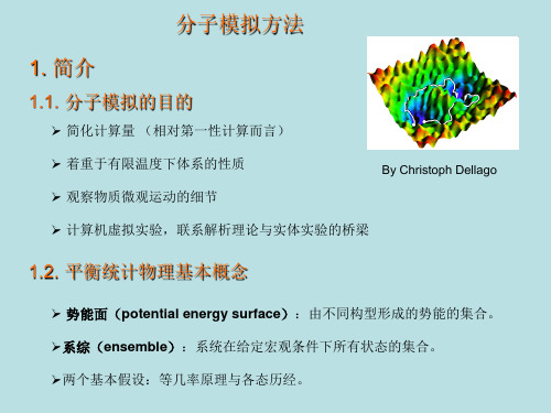
《分子模拟方法》课件

加速研发进程
分子模拟可以大大缩短药 物研发、材料合成等领域 的实验周期,降低研发成 本。
揭示微观机制
通过模拟,可以揭示分子 间的相互作用机制和反应 过程,有助于深入理解物 质的性质和行为。
分子模拟的发展历程
经典力学模拟
基于牛顿力学,适用于 较大分子体系,但精度
较低。
量子力学模拟
适用于小分子体系,精 度高,但计算量大,需
详细描述
利用分子模拟方法,模拟小分子药物与生物大分子(如蛋白质、核酸等)的相 互作用过程,探究药物的作用机制和药效,为新药研发提供理论支持。
高分子材料的模拟研究
总结词
研究高分子材料的结构和性能,优化 材料的设计和制备。
详细描述
通过模拟高分子材料的结构和性能, 探究高分子材料的物理和化学性质, 优化材料的设计和制备过程,为新材 料的研发提供理论指导。
分子动力学方法需要较高的计算资源和 精度,但可以获得较为准确的结果,因 此在计算化学、生物学、材料科学等领
域得到广泛应用。
介观模拟的原理
介观模拟是一种介于微观和宏观之间的模拟方 法,通过模拟一定数量的粒子的相互作用和演 化来研究介观尺度的结构和性质。
介观模拟方法通常采用格子波尔兹曼方法、粒 子流体动力学等方法,适用于模拟流体、表面 、界面等介观尺度的问题。
分子模拟基于量子力学、经典力 学、蒙特卡洛等理论,通过建立 数学模型来描述分子间的相互作
用和运动。
分子模拟可以用于药物研发、材 料科学、环境科学等领域,为实 验研究和工业应用提供重要支持
。
分子模拟的重要性
01
02
03
预测分子性质
通过模拟,可以预测分子 的性质,如稳定性、溶解 度、光谱等,为实验设计 和优化提供指导。
分子模拟课件
ME346–Introduction to Molecular Simulations–Stanford University–Winter2007 Handout1.An Overview of Molecular SimulationWei Caic All rights reservedSeptember26,2005Contents1Examples of molecular simulations1 2What consists of a molecular dynamics?2 3Newton’s equation of motion2 4A simple numerical integrator:Verlet algorithm5 1Examples of molecular simulationsPictures and movies of modern large scale molecular simulations can be downloaded from the course web site /∼me346(click“Course Materials”).Exam-ples include plastic deformation in metals containing a crack,phase transformation induced by shock waves,nano-indentation of metalfilm,laser ablation on metal surface,etc.In each of these examples,molecular simulations not only produce beautiful pictures,but they also offer new understanding on the behavior of materials at the nano-scale.Many times such understanding provides new insights on how the materials would behave at the micro-scale and nano-scale.With unique capabilities to offer,molecular simulation has become a widely used tool for scientific investigation that complements our traditional way of doing science: experiment and theory.The purpose of this course is to provide thefirst introduction to molecular level simulations—how do they work,what questions can they answer,and how much can we trust their results—so that the simulation tools are no longer black boxes to us.Students will develop a set of simulation codes in Matlab by themselves.(A simple Matlab tutorial written by Sigmon[5]may help you refresh your memory.)We will also give tutorial and exercise problems based on MD++,a molecular simulation package used in my research group.MD++will be used for illustration in class as well as tools to solve homework problems.2What consists of a molecular dynamics?In a molecular simulation,we view materials as a collection of discrete atoms.The atoms interact by exerting forces on each other and they follow the Newton’s equation of motion. Based on the interaction model,a simulation compute the atoms’trajectories numerically. Thus a molecular simulation necessarily contains the following ingredients.•The model that describes the interaction between atoms.This is usually called the interatomic potential:V({r i}),where{r i}represent the position of all atoms.•Numerical integrator that follows the atoms equation of motion.This is the heart of the ually,we also need auxiliary algorithms to set up the initial and bound-ary conditions and to monitor and control the systems state(such as temperature) during the simulation.•Extract useful data from the raw atomic trajectory pute materials properties of interest.Visualization.We will start our discussion with a simple but complete example that illustrates a lot of issues in simulation,although it is not on the molecular scale.We will simulate the orbit of the Earth around the Sun.After we have understood how this simulation works(in a couple of lectures),we will then discuss how molecular simulations differ from this type of “macro”-scale simulations.3Newton’s equation of motionThroughout this course,we limit our discussions to classical dynamics(no quantum mechan-ics).The dynamics of classical objects follow the three laws of Newton.Let’s review the Newton’s laws.Figure1:Sir Isaac Newton(1643-1727England).First law:Every object in a state of uniform motion tends to remain in that state of motion unless an external force is applied to it.This is also called the Law of inertia.Second law:An object’s mass m,its acceleration a,and the applied force F are related byF=m a.The bold font here emphasizes that the acceleration and force are vectors.Here they point to the same direction.According to Newton,a force causes only a change in velocity(v)but is not needed to maintain the velocity as Aristotle claimed(erroneously).Third law:For every action there is an equal and opposite reaction.The second law gives us the equation of motion for classical particles.Consider a particle (be it an atom or the Earth!depending on which scale we look at the world),its position is described by a vector r=(x,y,z).The velocity is how fast r changes with time and is also a vector:v=d r/dt=(v x,v y,v z).In component form,v x=dx/dt,v y=dy/dt,v z=dz/dt. The acceleration vector is then time derivative of velocity,i.e.,a=d v/dt.Therefore the particle’s equation of motion can be written asd2r dt2=Fm(1)To complete the equation of motion,we need to know how does the force F in turn depends on position r.As an example,consider the Earth orbiting around the Sun.Assume the Sun isfixed at origin(0,0,0).The gravitational force on the Earth is,F=−GmM|r|2·ˆe r(2)whereˆe r=r/|r|is the unit vector along r direction.|r|=√x2+y2+z2is the magnitudeof r.m is the mass of the Earth(5.9736×1024kg),M is mass of the Sun(1.9891×1030kg), and G=6.67259×10⁻¹¹N·m2/kg2is gravitational constant.If we introduce a potential field(the gravitationalfield of the Sun),V(r)=−GmM|r|(3)Then the gravitational force can be written as minus the spatial derivative of the potential,F=−dV(r)d r(4)In component form,this equation should be interpreted as,F x=−dV(x,y,z)dxF y=−dV(x,y,z)dyF z=−dV(x,y,z)dzNow we have the complete equation of motion for the Earth:d2r dt2=−1mdV(r)d r(5)in component form,this reads,d2x dt2=−GMx|r|3d2y dt2=−GMy|r|3d2z dt2=−GMz|r|3In fact,most of the system we will study has a interaction potential V(r),from which the equation of motion can be specified through Eq.(5).V(r)is the potential energy of the system.On the other hand,the kinetic energy is given by the velocity,E kin=12m|v|2(6)The total energy is the sum of potential and kinetic energy contributions,E tot=E kin+V(7) When we express the total energy as a function of particle position r and momentum p=m v, it is called the Hamiltonian of the system,H(r,p)=|p|22m+V(r)(8)The Hamiltonian(i.e.the total energy)is a conserved quantity as the particle moves.To see this,let us compute its time derivative,dE tot dt =m v·d vdt+dV(r)d r·d rdt=md rdt·−1mdV(r)d r+dV(r)d r·d rdt=0(9)Therefore the total energy is conserved if the particle follows the Newton’s equation of motion in a conservative forcefield(when force can be written in terms of spatial derivative of a potentialfield),while the kinetic energy and potential energy can interchange with each other.The Newton’s equation of motion can also be written in the Hamiltonian form,d r dt =∂H(r,p)∂p(10)d p dt =−∂H(r,p)∂r(11)Hence,dH dt =∂H(r,p)∂r·d rdt+∂H(r,p)∂p·d pdt=0(12)Figure2:Sir William Rowan Hamilton(1805-1865Ireland).4A simple numerical integrator:Verlet algorithmA dynamical simulation computes the particle position as a function of time(i.e.its trajec-tory)given its initial position and velocity.This is called the initial value problem(IVP). Because the Newton’s equation of motion is second order in r,the initial condition needs to specify both particle position and velocity.To solve the equation of motion on a computer,thefirst thing we need is to discretize the time.In other words,we will solve for r(t)on a series of time instances t ually the time axis is discretized uniformly:t i=i·∆t,where∆t is called the time step.Again,the task of the simulation algorithm is tofind r(t i)for i=1,2,3,···given r(0)and v(0).The Verlet algorithm begins by approximating d2r(t)/dt2,d2r(t) dt2≈r(t+∆t)−2r(t)+r(t−∆t)∆t2(13)Thusr(t+∆t)−2r(t)+r(t−∆t)∆t2=−1mdV(r(t))dr(14)r(t+∆t)=2r(t)−r(t−∆t)−∆t·1m·dV(r(t))dr(15)Therefore,we can solve r(t+∆t)as along as we know r(t)and r(t−∆t).In other words,if we know r(0)and r(−∆t),we can solve for all r(t i)for i=1,3,4,···.Question:Notice that to start the Verlet algorithm we need r(0)and r(−∆t).However, the initial condition of a simulation is usually given in r(0)and v(0).How do we start the simulation when this initial condition is specified?References1.Alan and Tildesley,Computer Simulation of Liquids,(Oxford University Press,1987)pp.71-80.2.Frenkel and Smit,Understanding Molecular Simulation:From Algorithms to Applica-tions,2nd ed.(Academic Press,2002).3.Bulatov and Cai,Computer Simulation of Dislocations,(Oxford University Press,2006)pp.49-51.ndau and Lifshitz,Mechanics,(Butterworth-Heinemann,1976).5.Kermit Sigmon,Matlab Primer,Third Edition,/Matlab/matlab-primer.pdfME346–Introduction to Molecular Simulations–Stanford University–Winter2007 Handout2.Numerical Integrators IWei Caic All rights reservedJanuary12,2007Contents1Which integrator to use?1 2Several versions of Verlet algorithm2 3Order of accuracy3 4Other integrators4 1Which integrator to use?In the previous lecture we looked at a very simple simulation.The Newton’s equation of motion is integrated numerically by the original Verlet algorithm.There are many algorithms that can be used to integrate an ordinary differential equation(ODE).Each has a its own advantages and disadvantages.In this lecture,we will look into more details at the numerical integrators.Our goal is to be able to make sensible choices when we need to select a numerical integrator for a specific simulation.What questions should we ask when choosing an integrator?Obviously,we would like something that is both fast and accurate.But usually there are more issues we should care about.Here are a list of the most important ones(Allen and Tildesley1987):•Order of accuracy•Range of stability•Reversibility•Speed(computation time per step)•Memory requirement(as low as possible)•Satisfying conservation law•Simple form and easy to implementItem1and2(especially2)are important to allow the use of long time steps,which makes the simulation more efficient.2Several versions of Verlet algorithmThe Verlet algorithm used in the previous lecture can be written as,r(t+∆t)=2r(t)−r(t−∆t)+a(t)·∆t2(1)wherea(t)=−1mdV(r(t))d r(t)(2)While this is enough to compute the entire trajectory of the particle,it does not specify the velocity of the particle.Many times,we would like to know the particle velocity as a function of time as well.For example,the velocity is needed to compute kinetic energy and hence the total energy of the system.One way to compute velocity is to use the followingapproximation,v(t)≡d r(t)dt≈r(t+∆t)−r(t−∆t)2∆t(3)Question:if the initial condition is given in terms of r(0)and v(0),how do we use the Verlet algorithm?Answer:The Verlet algorithm can be used to compute r(n∆t)for n=1,2,···provided r(−∆t)and r(0)are known.The task is to solve for r(−∆t)given r(0)and v(0).This is achieved from the following two equations,r(∆t)−r(−∆t)2∆t=v(0)(4)r(∆t)−2r(0)+r(−∆t)∆t2=−1mdV(r(t))d r(t)t=0(5)Exercise:express r(−∆t)and r(∆t)in terms of r(0)and v(0).Therefore,r(−∆t)and r(∆t)are solved together.During the simulation,we only know v(t)after we have computed(t+∆t).These are the(slight)inconveniences of the(original) Verlet algorithm.As we will see later,in this algorithm the accuracy of velocity calculation is not very high(not as high as particle positions).Several modifications of the Verlet algorithms were introduced to give a better treatment of velocities.The leap-frog algorithm works as follows,v(t+∆t/2)=v(t−∆t/2)+a(t)·∆t(6)r(t+∆t)=r(t)+v(t+∆t/2)·∆t(7) Notice that the velocity and position are not stored at the same time slices.Their values are updated in alternation,hence the name“leap-frog”.For a nice illustration see(Allen and Tildesley1987).This algorithm also has the draw back that v and r are not known simultaneously.To get velocity at time t,we can use the following approximation,v(t)≈v(t−∆t/2)+v(t+∆t/2)2(8)The velocity Verlet algorithm solves this problem in a better way.The algorithm reads,r(t+∆t)=r(t)+v(t)∆t+12a(t)∆t2(9)v(t+∆t/2)=v(t)+12a(t)∆t(10)a(t+∆t)=−1mdV(r(t+∆t))d r(t+∆t)(11)v(t+∆t)=v(t+∆t/2)+12a(t+∆t)∆t(12)Exercise:show that both leap-frog and velocity Verlet algorithms gives identical results as the original Verlet algorithm(except forfloating point truncation error).3Order of accuracyHow accurate are the Verlet-family algorithms?Let’s take a look at the original Verletfirst. Consider the trajectory of the particle as a continuous function of time,i.e.r(t).Let us Taylor expand this function around a given time t.r(t+∆t)=r(t)+d r(t)dt∆t+12d2r(t)dt2∆t2+13!d3r(t)dt3∆t3+O(∆t4),(13)where O(∆t4)means that error of this expression is on the order of∆t4.In other words, (when∆t is sufficiently small)if we reduce∆t by10times,the error term would reduce by 104times.Replace∆t by−∆t in the above equation,we have,r(t−∆t)=r(t)−d r(t)dt∆t+12d2r(t)dt2∆t2−13!d3r(t)dt3∆t3+O(∆t4),(14)Summing the two equations together,we have,r(t+∆t)+r(t−∆t)=2r(t)+d2r(t)dt2∆t2+O(∆t4)≡2r(t)+a(t)∆t2+O(∆t4)(15)r(t+∆t)=2r(t)−r(t−∆t)+a(t)∆t2+O(∆t4)(16) Therefore,the local accuracy for the Verlet-family algorithms is to the order of O(∆t4). This is quite accurate for such a simple algorithm!The trick here is that,by adding t+∆t and t−∆t terms,the third order term cancels out.Notice that the accuracy analysis here deals with the local error.That is,assuming r(t)is exact,how much error we make when computing r(t+∆t).In practice,the total error of computed r at time t is the accumulated (and possibly amplified)effect of all time steps before time t.Because for a smaller timestep ∆t more steps is required to reach a pre-specified time t,the global order of accuracy is always local order of accuracy minus one.For example,the global order of accuracy for Verlet algorithms is3.Since all Verlet-family algorithms generate the same trajectory,they are all O(∆t4)in terms of particle positions.But they differ in velocity calculations.How accurate is the velocity calculation in the original Verlet algorithm?Let us subtract Eq.(13)and(14),r(t+∆t)−r(t−∆t)=2v(t)∆t+13d3r(t)dt3∆t3+O(∆t4),(17)v(t)=12∆tr(t+∆t)−r(t−∆t)−16d3r(t)dt2∆t3+O(∆t3)(18)v(t)=r(t+∆t)−r(t−∆t)2∆t+O(∆t2)(19)Thus the velocity is only accurate to the order of O(∆t2)!This is much worse than O(∆t4) of the positions.A reason for the lose of accuracy is that the velocities are computed by taking the difference between two large numbers,i.e.r(t+∆t)and r(t−∆t),and then divide by a small number.1Intuitively,higher order algorithms allows the use of bigger time steps to achieve the same level of accuracy.However,the more important determining factor for the choice of time steps is usually not the order of accuracy,but instead is the algorithm’s numerical stability (see next section).4Other integratorsBefore closing this lecture,let us briefly look at two other well known integrators.Gear’s predictor-corrector method is a high-order integrator.It keeps track of several time deriva-tives of the particle position.Definer0(t)≡r(t)(20) 1Strictly speaking,Eq.(17)is valid when we have exact values for r(t+∆t),r(t)and r(t−∆t).But in doing the order-of-accuracy analysis,we can only assume that we have exact values for r(t)and r(t−∆t) and we know that we are making an error in r(t+∆t).Fortunately,the error we make in r(t+∆t)is also O(∆t4).Thus Eq.(17)still holds.r1(t)≡∆t d r(t)dt(21)r2(t)≡∆t22!d2r(t)dt2(22)r3(t)≡∆t33!d3r(t)dt3(23)···Sincer(t+∆t)=r(t)+∆t d r(t)dt+∆t22!d2r(t)dt2+∆t33!d3r(t)dt3+O(∆t4)=r(t)+r1(t)+r2(t)+r3(t)+O(∆t4)r1(t+∆t)=r1(t)+2r2(t)+3r3(t)+O(∆t4)r2(t+∆t)=r2(t)+3r3(t)+O(∆t4)r3(t+∆t)=r3(t)+O(∆t4)we can predict the values of r and r i at time t+∆t simply based on their values at time t,r P(t+∆t)=r(t)+r1(t)+r2(t)+r3(t)r P1(t+∆t)=r1(t)+2r2(t)+3r3(t)r P2(t+∆t)=r2(t)+3r3(t)r P3(t+∆t)=r3(t)Notice that we have not even calculated the force at all!If we compute the force at time t+∆t based on the predicted position r P(t+∆t),we will obtain the second derivative of r at time t+∆t—let it be r C(t+∆t).Mostly likely,r C(t+∆t)will be different from the predicted value r P(t+∆t).Thefinal results are obtained by adding a correction term to each predictor,r n(t+∆t)=r Pn (t+∆t)+C n[r C2(t+∆t)−r P2(t+∆t)](24)The Gear’s6th order scheme(uses r0through r5)takes the following C n values,C0=3 16C1=251 360C2=1C3=11 18C4=1 6C5=1 60The global accuracy is of the order O(∆t)6,hence the method is called the Gear’s6th order algorithm.Exercise:show that the local truncation error of the above scheme is of the order of O (∆t 7).In a way,the Runge-Kutta method is similar to predictor-corrector methods in that the final answer is produced by improving upon previous predictions.However,the Runge-Kutta method requires multiple evaluation of forces.The Runge-Kutta method is most conveniently represented when the equation of motion is written as a first order differential equation,˙η=g (η)≡ω∂H (η)∂η(25)whereη≡(r ,p )(26)andω= 0I−I 0 (27)and I is the 3×3identity matrix and H is the Hamiltonian.The fourth-order Runge-Kutta method goes as (from ),k 1=∆t ·g (η(t ))k 2=∆t ·g η(t )+12k 1 k 3=∆t ·g η(t )+12k 2 k 4=∆t ·g (η(t )+k 3)η(t +∆t )=η(t )+16k 1+13k 2+13k 3+16k 4(28)Exercise:show that the local truncation error of the above scheme is of the order of O (∆t 5)and the global accuracy is of the order of O (∆t 4).Suggested reading1.(Alan and Tildesley 1987)pp.71-84.2.J.C.Butcher,The numerical analysis of ordinary differential equations:Runge-Kutta and general linear methods ,(Wiley,1987),pp.105-151.ME346–Introduction to Molecular Simulations–Stanford University–Winter2007 Handout3.Symplectic ConditionWei Caic All rights reservedJanuary17,2007Contents1Conservation laws of Hamiltonian systems1 2Symplectic methods4 3Reversibility and chaos5 4Energy conservation7 1Conservation laws of Hamiltonian systemsThe numerical integrators for simulating the Newton’s equation of motion are solvers of ordinary differential equations(ODE).However,the Newton’s equation of motion that can be derived from a Hamiltonian is a special type of ODE(not every ODE can be derived from a Hamiltonian).For example,a Hamiltonian system conserves it total energy,while an arbitrary ODE may not have any conserved quantity.Therefore,special attention is needed to select an ODE solver for Molecular Dynamics simulations.We need to pick those ODE solvers that obeys the conservation laws of a Hamiltonian system.For example,if an ODE solver predicts that the Earth will drop into the Sun after100cycles around the Sun,it is certainly the ODE solver to blame and we should not immediately start worrying about the fate of our planet based on this prediction.A conservation law is a(time invariant)symmetry.A Hamiltonian system possess more symmetries than just energy conservation.Ideally the numerical integration scheme we pick should satisfy all the symmetries of the true dynamics of the system.We will look at these symmetries in this and following sections.When discussing a Hamiltonian system,it is customary to use letter q to represent the particle position(instead of r).Recall that the equation of motion for a system with Hamiltonian H(q,p)is,˙q=∂H(q,p)∂p(1)˙p=−∂H(q,p)∂q,(2)where˙q≡d q/dt,˙p≡d p/dt.If the system has N particles,then q is a3N-dimensional vector specifying its position and p is a3N-dimensional vector specifying its momentum. (In the above Earth orbiting example,N=1.)Notice that in terms of q and p,the equation of motion is a set of(coupled)first-order differential equations(whereas F=m a is second order).The equation can be reduced to an even simpler form if we define a6N-dimensional vectorη≡(q,p)(3) Then the equation of motion becomes,˙η=ω∂H(η)∂η(4)whereω=0I−I0(5)and I is the3×3identity matrix.The6N-dimensional space whichη≡(q,p)belongs to is called the phase space.The evolution of system in time can be regarded as the motion of a pointηin the6N-dimensional phase space following thefirst-order differential equation(4).(a)(b)Figure1:(a)Motion of a point(q,p)in phase space is confined to a shell with constant energy.(b)Area of a phase space element(shaded)is conserved.Because the Newton’s equation of motion conserves total energy,the motion of a point in phase space must be confined to a subspace(or hyperplane)with constant energy,i.e.a constant energy shell,as illustrated in Fig.1(a).Think about all the points in the constant energy shell.As time evolves,the entire volume that these points occupy remains the same —the points simply rearrange within the constant energy shell.Let us now consider the evolution of a small element in phase space over time,as illus-trated in Fig.1(b).Think of this as the ensemble of trajectories of many Molecular Dynamics simulations with very similar initial conditions.We will show that the area enclosed by this element remains constant,even though the element inevitably experiences translation anddistortion.1Let the element at time t be a hypercube around pointη,whose area is,|dη|=|d q|·|d p|=dq1···dq3N dp1···dp3N(6) For a pointηat time t,letξbe its new position at time t+δt.In the limit ofδt→0,wehave,ξ=η+˙ηδt=η+ω∂H(η)∂ηδt(7)Because the above equation is true only in the limit ofδt→0,we will ignore any higher order terms(e.g.δt2)in the following discussions.Let M be the Jacobian matrix of the transformation fromηtoξ,i.e.,M≡∂ξ∂η=1+ω∂2H(η)∂η∂ηδt(8)For clarity,we write M explicitly in terms of q and p,M=1+0I−I0·∂2H∂q∂q∂2H∂q∂p∂2H∂p∂q∂2H∂p∂p·δt(9)=1+∂2Hδt∂2Hδt−∂2H∂q∂qδt1−∂2H∂q∂pδt(10)The area of the new element is related to the the determinant of the Jacobian matrix,|dξ|=|dη|·|det M|=|dη|·(1+O(δt2))(11) Because thefirst order term ofδt in det M vanishes,we can show that the area of the element remains constant for an arbitrary period of time(i.e.forever).2This is an important property of a Hamiltonian system.Because the area of any element in phase space always remains constant,the evolution of phase space points is analogous to that in an incompressiblefluid.Exercise:Write down the explicit expression for the Jacobian matrix M for problem of the Earth orbiting around the Sun.The Hamiltonian dynamics has even more symmetries.Notice that the transpose of M is,M T=1−∂2H∂η∂ηωδt(12)1It then follows that the area enclosed by an arbitrarily shaped element in the phase space also remains constant.2To show that area remains constant after afinite period∆t,we only need to divide the time interval into N subintervals,each withδt=∆t/N.The area change per subinterval is of the order of1/N2.The accumulated area change over time period∆t is then of the order of1/N,which vanishes as N→∞.we haveM ωM T = 1+ω∂2H ∂η∂ηδt ω 1−∂2H ∂η∂ηωδt =ω+ω∂2H ∂η∂ηωδt −ω∂2H ∂η∂ηωδt +O (δt 2)(13)=ω+O (δt 2)(14)(15)Therefore the Jacobian matrix M thus satisfies the so called symplectic condition (up to O (δt 2)),M ωM T =ω(16)Again,we can show that the symplectic condition is satisfied for an arbitrary period of time.To be specific,let ξbe the point in phase space at time t ;at time 0this point was at η.ξcan then be regarded as a function of t and η(initial condition),i.e.ξ=ξ(η,t ).Define M as the Jacobian matrix between ξand η,we can show that M satisfies the symplectic condition Eq.(16).3Obviously,the Hamiltonian dynamics is also time reversible.This means that if ηevolves to ξafter time t .Another phase space point η that has the same q as ηbut with reversed p (momentum)will exactly come to point ξafter time t .To summarize,the dynamics of a system that has a Hamiltonian has the following symmetry properties:•Conserves total energy•Conserves phase space area (incompressible flow in phase space)•Satisfies symplectic condition Eq.(16)•Is time reversibleIdeally,the numerical integrator we choose to simulate Hamiltonian system should satisfy all of these symmetries.In the following,let us take a look at how specific integrators are doing in this regard.In fact,if an algorithm satisfies the symplectic condition,it automatically conserves phase space area 4,is reversible,and should have good long-term energy conserva-tion properties.This is why symplectic methods are good choices for simulating Hamiltonian systems.2Symplectic methodsWhat do we mean if we ask whether a numerical integrator satisfies the symplectic condition or not?For a numerical integrator,the system moves forward in time by discrete jumps.Let3Again,we devide the time period t into N subintervals,each with δt =∆t/N .Let M i be the Jacobian matrix from time (i −1)δt to iδt .We have M = N i =1M i .We can show that M T ωM =ωin the limit of N →∞.4Since M T ωM =ω,det ω=det(M T ωM )=(det M )2det ω.Thus det M =±1,which means area conservation.η(i)=(q(i),p(i))be the place of the system in the phase space at time step i,i.e.t i=i∆t. At the next time step,the algorithm brings the system to pointη(i+1)=(q(i+1),p(i+1)). Let M be the Jacobian matrix that connectsη(i)withη(i+1).The method is symplectic if MωM T=ω.The good news is that the Verlet-family algorithms are symplectic.To show this is the case,let us consider the leap-frog algorithm.Let q(i)correspond to q(i·∆t)and p(i) correspond to p((i−12)·∆t).Then the leap-frog algorithm is,p(i+1)=p(i)−∂V∂q(i)∆t(17)q(i+1)=q(i)+p(i+1)m∆t=q(i)+1mp(i)−∂V∂q(i)∆t∆t(18)Thus,M=∂q(i+1)∂q(i)∂q(i+1)∂p(i)∂p(i+1)(i)∂q(i+1)(i)=1−1m∂2V∂q(i)∂q(i)∆t2∆tm−∂2V∂q(i)∂q(i)∆t1(19)Thus M is symplectic.Exercise:show that for M defined in Eq.(19),MωM T=ω(symplectic)and det M=1 (area preserving).Exercise:derive the Jacobian matrix M for velocity Verlet algorithm and show that it is symplectic and area preserving.3Reversibility and chaosBecause the Verlet-family algorithms(original Verlet,leap-frog and velocity Verlet)are sym-plectic,they are also time reversible.Nonetheless,it is instructive to show the time reversibil-ity explicitly.If we run the leap-frog algorithm in reverse time,then the iteration can be written as,˜q(i+1)=˜q(i)+˜p(i)m∆t(20)˜p(i+1)=˜p(i)−∂V∂q(i+1)∆t(21)(22)where i is the iteration number,˜q(i)=q(−i∆t),˜p(i)=p((−i−12)∆t).It is not difficult toshow that if˜q(i)=q(i+1)and˜p(i)=−p(i+1),then˜q(i+1)=q(i)and˜p(i+1)=−p(i).Exercise:show that the leap-frog algorithm is reversible.Exercise:show that the velocity Verlet algorithm is reversible.Exercise:show that the Forward Euler method:q(i+1)=q(i)+∆t·p(i)/m,p(i+1)=p(i)−∆t·∂V/∂q(i),is not reversible and not symplectic.Since every integration step using the Verlet algorithm is time reversible,then in principle an entire trajectory of Molecular Dynamics simulation using the Verlet algorithm should be time reversible.To be specific,let the initial condition of the simulation be q(0)and p(0). After N steps of integration,the system evolves to point q(N)and p(N).Time reversibility means that,if we run the reverse Verlet iteration starting from q(N)and−p(N),after N steps we should get exactly to point q(0)and−p(0).In practice,however,we never have perfect reversibility.This is due to the combined effect of numerical round offerror and the chaotic nature of trajectories of many Hamiltonian systems.The chaotic nature of many Hamiltonian system can be illustrated by considering the two trajectories with very close initial conditions.Let the distance between the two points in phase space at time0be d(0).At sufficiently large t,the two phase space points will diverge exponentially,i.e.d(t)∼d(0)eλt,whereλis called the Lyapunov exponent and this behavior is called Lyapunov instability.Given that we can only represent a real number on a computer withfinite precision,we are in effect introducing a small(random) perturbation at every step of the integration.Therefore,sooner or later,the numerical trajectory will deviate from the analytical trajectory(if the computer had infinite precision) significantly5.While the analytical trajectory is reversible,the one generated by a computer is not.This is why there exist a maximum number of iterations N,beyond which the original state cannot be recovered by running the simulation backwards.This by itself does not present too big a problem,since we seldom have the need to recover the initial condition of the simulation in this way.However,this behavior does mean that we will not be able to follow the“true”trajectory of the original system forever on a computer.Sooner or later, the“true”trajectory and the simulated one will diverge significantly.This is certainly a problem if we would like to rely entirely on simulations to tell us where is our satellite or space explorer.However,this usually does not present a problem in Molecular Simulations, in which we are usually not interested in the exact trajectories of every atom.We will return to this point in future lectures when we discuss Molecular Dynamics simulations involving many atoms.5Notice that the analytical trajectory here is not the same as the“true”trajectory of the original system. The analytical trajectory is obtained by advancing the system in discrete jumps along the time axis.。
分子模拟教案—

教案课程名称分子模拟授课题目(章、节) 第一章授课教师李慎敏授课对象化学081-2 授课时间9月2日教学方法讲授选用教具多媒体本教案以讲授一个单元(2—4学时)或一次实验(实习)为单位填写。
填写要用钢笔,字迹要清晰、工整。
按表项目逐一填写。
教案课程名称分子模拟授课题目(章、节) 第二章授课教师李慎敏授课对象化学081-2 授课时间9月9日教学方法讲授选用教具多媒体本教案以讲授一个单元(2—4学时)或一次实验(实习)为单位填写。
填写要用钢笔,字迹要清晰、工整。
按表项目逐一填写。
教案课程名称分子模拟授课题目(章、节) 第三章授课教师李慎敏授课对象化学081-2 授课时间9月16 日教学方法讲授选用教具多媒体本教案以讲授一个单元(2—4学时)或一次实验(实习)为单位填写。
填写要用钢笔,字迹要清晰、工整。
按表项目逐一填写。
教案课程名称分子模拟授课题目(章、节) 第三章授课教师李慎敏授课对象化学081-2 授课时间9月23 日教学方法讲授选用教具多媒体本教案以讲授一个单元(2—4学时)或一次实验(实习)为单位填写。
填写要用钢笔,字迹要清晰、工整。
按表项目逐一填写。
教案课程名称分子模拟授课题目(章、节) 第四章授课教师李慎敏授课对象化学081-2 授课时间10月9日教学方法讲授选用教具多媒体本教案以讲授一个单元(2—4学时)或一次实验(实习)为单位填写。
填写要用钢笔,字迹要清晰、工整。
按表项目逐一填写。
教案课程名称分子模拟授课题目(章、节) 第四章授课教师李慎敏授课对象化学081-2 授课时间10月14日教学方法讲授选用教具多媒体本教案以讲授一个单元(2—4学时)或一次实验(实习)为单位填写。
填写要用钢笔,字迹要清晰、工整。
按表项目逐一填写。
教案课程名称分子模拟授课题目(章、节) 第五章授课教师李慎敏授课对象化学081-2 授课时间10月21 日教学方法讲授选用教具多媒体本教案以讲授一个单元(2—4学时)或一次实验(实习)为单位填写。
《分子模拟设计》课件

目录
• 分子模拟设计概述 • 分子模拟设计的基本方法 • 分子模拟设计的应用领域 • 分子模拟设计的挑战与展望 • 分子模拟设计案例分析
01
CATALOGUE
分子模拟设计概述
定义与特点
定义
分子模拟设计是指利用计算机模 拟技术,对分子结构和性质进行 预测和设计的过程。
蒙特卡洛模拟
总结词
基于概率统计的模拟方法
详细描述
蒙特卡洛模拟是一种基于概率统计的模拟方法,通过随机抽样和统计计算来获 得系统的性质。该方法适用于模拟复杂系统,能够考虑系统的随机性和不确定 性。
分子力学模拟
总结词
基于势能函数的模拟方法
详细描述
分子力学模拟是一种基于势能函数的模拟方法,通过势能函数来描述分子间的相互作用和分子结构。该方法适用 于快速计算分子的结构和性质,常用于药物设计和材料科学等领域。
材料的界面行为等多个方面。
高分子材料的模拟设计有助于缩短新材料研发周期、 降低研发成本,提高新材料开发的成功率。
高分子材料的模拟设计是利用分子模拟技术对 高分子材料的结构和性质进行预测和优化的一 种方法。
通过模拟高分子材料的结构和性质,可以预测材 料的力学性能、热性能、电性能等,从而优化材 料的设计和制备工艺。
在生物大分子模拟中,研究人员可以使用分子模拟设计来研究蛋白质、 核酸和糖等生物大分子的结构和动力学性质。
这有助于理解这些大分子在细胞中的功能和相互作用的机制,以及与疾 病相关的生物大分子的异常行为。
04
CATALOGUE
分子模拟设计的挑战与展望
计算资源的限制
计算资源不足
高性能计算机和计算集群的资源有限,难以满足 大规模分子模拟的需求。
分子动力学模拟I
Gromacs中文教程淮海一粟分子动力学(MD)模拟分为三步:首先,要准备好模拟系统;然后,对准备好的系统进行模拟;最后,对模拟结果进行分析。
虽然第二步是最耗费计算资源的,有时候需要计算几个月,但是最耗费体力的步骤在于模拟系统准备和结果分析。
本教程涉及模拟系统准备、模拟和结果分析。
一、数据格式处理准备好模拟系统是MD最重要的步骤之一。
MD模拟原子尺度的动力学过程,可用于理解实验现象、验证理论假说,或者为一个待验证的新假说提供基础。
然而,对于上述各种情形,都需要根据实际情况对模拟过程进行设计;这意味着模拟的时候必须十分小心。
丢失的残基、原子和非标准基团本教程模拟的是蛋白质。
首先需要找到蛋白质序列并选择其起始结构,见前述;然后就要检查这个结构是否包含所有的残基和原子,这些残基和原子有时候也是模拟所必需的。
本教程假定不存在缺失,故略去。
另一个需要注意的问题是结构文件中可能包含非标准残基,被修饰过的残基或者配体,这些基团还没有力场参数。
如果有这些基团,要么被除去,要么就需要补充力场参数,这牵涉到MD的高级技巧。
本教程假定所有的蛋白质不含这类残基。
结构质量对结构文件进行检查以了解结构文件的质量是一个很好的练习。
例如,晶体结构解析过程中,对于谷氨酰胺和天冬酰胺有可能产生不正确的构象;对于组氨酸的质子化状态和侧链构象的解析也可能有问题。
为了得到正确的结构,可以利用一些程序和服务器(如WHATIF)。
本教程假定所用的结构没有问题,我们只进行数据格式处理。
二、结构转换和拓扑化一个分子可以由各个原子的坐标、键接情况与非键相互作用来确定。
由于.pdb结构文件只含有原子坐标,我们首先必须建立拓扑文件,该文件描述了原子类型、电荷、成键情况等信息。
拓扑文件对应着一种力场,选择何种力场对于拓扑文件的建立是一个值得仔细考虑的问题。
这里我们用的是GROMOS96 53a6连接原子力场,该力场对于氨基酸侧链的自由能预测较好,并且与NMR试验结果较吻合。
《分子模拟教程》课件

人工智能和机器学习技术将在分子模拟中发挥越 来越重要的作用,例如用于优化模拟参数、预测 性质等。
多尺度模拟
目前分子模拟主要集中在原子或分子级别,未来 将进一步发展多尺度模拟方法,将微观尺度和宏 观尺度相结合,以更全面地理解物质性质和行为 。
跨学科融合
分子模拟将与生物学、医学、材料科学等更多学 科领域进行交叉融合,为解决实际问题提供更多 可能性。
环境科学
在环境科学领域,分子模拟可用于研究污 染物在环境中的迁移转化机制,为环境保 护提供理论依据。
THANKS.
分子动力学模拟的常见算法
Verlet算法
一种基于离散时间步长的算法,用于计算分子位置和速度。
leapfrog算法
一种常用的分子动力学模拟算法,具有数值稳定性和计算效率高的特 点。
Parrinello-Rahman算法
一种基于分子力场的算法,可以用于模拟大尺度分子体系的运动。
Langevin动力学算法
材料科学
通过模拟材料中分子的运动和相互作 用,可以研究材料的力学、热学和电 学等性质,为材料设计和优化提供依 据。
03
Monte Carlo模拟
Monte Carlo模拟的基本概念
随机抽样
Monte Carlo模拟基于随 机抽样的方法,通过大量 随机样本的统计结果来逼 近真实结果。
概率模型
Monte Carlo模拟建立概 率模型,模拟系统的状态 变化和行为。
通过模拟药物分子与靶点分子的相互作用,预测 药物活性并优化药物设计。
材料科学
研究材料中分子的结构和性质,预测材料的物理 和化学性质。
生物大分子模拟
模拟生物大分子的结构和动力学行为,如蛋白质 、核酸等,有助于理解其功能和性质。
分子模拟PPT—第一章 概论

对1998 年诺贝尔化学奖 划时代的评价
瑞典皇家科学院的评价:
“ ··量子化学已发展成为广大化学家都能使用 · 的工具,将化学带入一个新时代 — 实验 与理论能携手协力揭示分子体系的性质。 化学不再是一门纯实验科学了”
I2 在 光 滑 球 模 型
不 Ar 同溶 半剂 径中 光的 滑振 球动 内弛 豫 时 间
Radius / nm 1.2 1.5 1.8 2.2 Shift / cm-1 1.20 1.79 1.76 1.75
受限于不同半径的光滑球内I2在Ar溶剂中的振动光谱位移
单 壁 碳 纳 米 管 模 型
Radius / nm Shift / cm-1
0.68 (10,10)
1.02 (15,15) 1.36 (20,20) 1.70 (25,25) 2.04 (30,30)
3.42
3.53 3.54 3.55 3.55
受限于不同半径的碳纳米管内I2在 Ar溶剂中的振动光谱位移密度为0.5 g/cm3
纳米反应器
自然界生命体系中的化学变化 绝佳的反应环境
R
+
R
R
R R
product shape selectivity
• “三十年前,如果说并非大多数化学家,那末至少 是有许多化学家嘲笑量子化学研究,认为这些工 作对化学用处不大,甚至几乎完全无用。现在的 情况却是完全两样了…。当90年代行将结束之际, 我们看到化学理论和计算研究的巨大进展,导致 整个化学正在经历一场革命性的变化。Kohn和 Pople是其中的两位最优秀代表”
1986:李远哲:“ 在十五年前,如果理论 结果与实验有矛盾,那么经常证明是理论结果错 了。但是最近十年则相反,常常是实验错了。… 量子力学有些结果是实验工作者事先未想到的,
结构生物学大分子模拟课件

现在学习的是第12页,共69页
到2007年3月,已知的蛋白质序列超过60万 条,而测定了三维结构的蛋白质仅为4万多个
蛋白质三维结构的测定已经成为生命科学 发展的“瓶颈”
现在学习的是第13页,共69页
蛋白质结构的基本概念
蛋白质的二级结构单元 – a螺旋 – b折叠股(b-strand)和b折叠片(b-sheet)
Turns Random coil (its neither!)
现在学习的是第18页,共69页
酰胺平面
肽键的键长介于单键和双键之间,具有部分双键的性质,不能自由旋转。
现在学习的是第19页,共69页
a螺旋
α-螺旋结构
最常见、含量最丰富的二级结构
现在学习的是第20页,共69页
现在学习的是第21页,共69页
现在学习的是第35页,共69页
蛋白质分子表面的环区域
现在学习的是第36页,共69页
蛋白质分子表面的环区域(LOOP)
大多数蛋白质分子是由a-螺旋和/或b回折构成的。这些a-螺旋和/
或b回折通常由不同长度和不规则形状的环区域相连接。 螺旋与回折的组合形成了分子的稳定的疏水内核,环区
域位于分子的表面。主链上的这环区域的C=O和NH基团一
特点:不依赖于已知的结构模式,是一种普适的解 决方法,目前尚处于探索阶段
现在学习的是第42页,共69页
同源和比较模建方法
根据蛋白质结构的相似性,以已知蛋白质的结构为 模板构建未知蛋白质的三维结构
– 在进化过程中蛋白质三维结构的保守性远大 于序列的保守性,当两个蛋白质的序列同源 性/相似性高于35%时,一般情况下它们的三 维结构基本相同
针对局域能量极小,不是整个系统 能够计算含有大量原子的体系 简单有效,目前应用得最广泛
《分子模拟教程》课件

通过模拟分子的运动,研究分子在不同组态下的性质和行为。
2 蒙特卡洛模拟
使用随机抽样和统计方法,模拟分子在不同条件下的状态和性质。
3 量子化学计算
基于量子力学的数值计算方法,研究分子的结构和能量。
分子模拟在材料科学中的应用
材料设计
通过模拟分子的结构和性质,优化材料的性能和功能,加速新材料的研发。
《分子模拟教程》PPT课 件
本课件介绍了《分子模拟教程》的目的和内容,以及分子模拟在不同领域的 应用。
分子模拟的定义
分子模拟是利用计算机模拟分子和材料的行为和性质的过程。它可以帮助我们深入了解分子的结构、动 力学和相互作用。
分子模拟的基本原理
分子模拟基于物理和化学的基本原理,使用数值方法对分子进行模拟,考虑分子之间的相互作用和运动 规律。
界面和表面研究
模拟分子在材料表面和界面上的相互作用,深入了解材料的表面性质和反应过程。
电子器件模拟
通过分子模拟,优化电子器件的结构和性能,提高器件的效率和稳定性。
分子模拟在生物科学中的应用
蛋白质折叠
模拟蛋白质的折叠过程,揭示 其结构和功能之间的关系。
药物研发
通过分子模拟,筛选和设计新 药物,加速药物研发的过程。
细胞膜相互作用
研究分子在细胞膜上的相互作 用,理解细胞过程的基本机制。
结论和总结
分子模拟是一项重要的科学工具,可以帮助我们深入了解分子和材料的行为 和性质,推动科学研究和工程应用的发展。
分子模拟方法演示教学
常用热力学量
➢ 动能
Ek
N i1
1 2
mi vi2
➢ 温度 ➢ 势能 ➢ 压强
T 1
dNkB
N
mivi2
i1
其中 d 是空间维数
N
Ep =
E pi
i 1
p=kBTN 1
V dV
fijgrij
i<j
பைடு நூலகம்➢焓
H=E+pV
可以理解为 NPT 下的有效总内能
➢ 熵 S=kBln N ,V,E 其中 Ω是系统的总微观状态数
常用系综
➢ 微正则系综 (Microcanonical Ensemble): NVE 皆为常数。 ➢ 正则系综 (Canonical Ensemble): NVT 皆为常数。 ➢ 巨正则系综 (Grandcanonical Ensemble): μVT 皆为常数,粒子数不固定。 ➢ 等压-等温系综 (Isobaric-Isothermal Ensemble): NPT 皆为常数。 ➢ 等张力-等温系综 (Isotension-Isothermal Ensemble): 模拟盒子的形状可变。
➢ 等几率原理(principle of equal weights):一个热力学体系有相同的几率访 问每一个微观态(注意:不是能量的等几率!一个能量一般会对应很多微观 态)。由等几率原理推导得出 Boltzmann 分布:
Pj exp(Ej)/Q
其中配分函数(partition function) Q ex p ( E i) kB T
i
➢ 各态历经(egodicity):只要系统演化无穷长时间,总有几率历经势能面上 的所有点。即在极限情况下,系综平均和时间平均是等价的。
分子模拟第一章
分子模拟
牛继南
•分子模拟的作用
①模拟材料的结构 ②计算材料的性质 ③预测材料行为 ④验证试验结果(重现试 验过程) ⑤从微观角度认识材料 总之,是为了更深层次 理解结构,认识各种行 为.
• 分子模拟的优势: 可以降低试验成本
具有较高的安全性
实现通常条件下较难或无法进行的试验
超低温(低于-100℃)
超高压(大于100Mpa)
Engineering Village Search query: (molecular simulation) Author affiliation
• • • • • • • • • • • • • • • • • • • • • • Department Of Chemistry, University Of California 223 Sandia National Laboratories 179 Univ Of California 138 Theoretical Division, Los Alamos National Laboratory 114 Department Of Chemical Engineering, University Of California 109 Lawrence Livermore National Laboratory 108 Department Of Chemistry, University Of Cambridge 103 Los Alamos National Laboratory 98 Pacific Northwest National Laboratory 75 Department Of Chemistry, Stanford University 74 Department Of Engineering Mechanics, Tsinghua University 73 Department Of Chemical Engineering, Vanderbilt University 72 Accelerator Laboratory, University Of Helsinki 72 Department Of Chemical Engineering, Princeton University 71 Kyoto Univ 71 Department Of Chemistry, Northwestern University 71 Pennsylvania State Univ 70 Department Of Chemistry, New York University 69 Aiaa 69 Department Of Chemistry And Biochemistry, University Of California 66 Cornell Univ 65 Department Of Chemical And Biomolecular Engineering, National University Of Singapore 64 Centre For Molecular Simulation, Swinburne University Of Technology 63 Lawrence Livermore Natl. Laboratory 62 Osaka Univ 62 Department Of Physics And Astronomy, University College London 62 Department Of Chemistry, Princeton University 62 Department Of Chemistry, Columbia University 61 Department Of Chemical Engineering, University Of Massachusetts 61 Massachusetts Inst Of Technology 61 Institute For Materials Research, Tohoku University 60 • • • • • • • • • • • • • • • • • • • • • • • • • • • • Department Of Chemical Engineering, University Of Michigan 60 Materials Science Division, Argonne National Laboratory 60 Tohoku Univ 59 Department Of Chemistry, Indian Institute Of Technology 59 Division Of Physical Chemistry, Arrhenius Laboratory, Stockholm University 57 Department Of Chemical Engineering, Massachusetts Institute Of Technology 57 Center For Molecular Modeling, Department Of Chemistry, University Of Pennsylvania 56 Department Of Chemical Engineering, Tsinghua University 56 Division Of Engineering, Brown University 55 Department Of Chemistry, University College London 55 Institute Of Fluid Science, Tohoku University 55 Institute Of Physics, University Of Silesia 55 School Of Materials Science And Engineering, Georgia Institute Of Technology 54 Research School Of Chemistry, Australian National University 54 Ieee 53 Department Of Chemistry, University Of Michigan 53 Institut Laue-Langevin 53 Department Of Materials Science And Engineering, University Of Florida 52 Oak Ridge National Laboratory 52 Max-Planck-Institut Fur Polymerforschung 51 Univ Of Tokyo 50 Argonne National Laboratory 50 Department Of Chemical Engineering, University Of Tennessee 49 Department Of Chemistry, Zhejiang University 49 Graduate School, Chinese Academy Of Sciences 48 Department Of Mechanical Engineering, University Of Tokyo 47 Department Of Biochemistry, University Of Oxford 46 Center For Polymer Studies, Department Of Physics, Boston University 44 Univ Of Michigan 38
生物大分子结构模拟实验PPT课件
(一)三级结构 • 定义
整条肽链中全部氨基酸残基的相对空间位置。 即肽链中所有原子或基团在三维空间的排布位置。
•主要化学键:
疏水作用、离子键、氢键和 范德华力等
24
•三级结构的主要特点:
A.含多种二级结构单元 B. 有明显的折叠层次 C. 是紧密的球状或椭球状实体 D.分子表面有一空穴(活性部位) E. 疏水侧链埋藏在分子内部
纤连蛋白分子的结构域
27
• 结构域(domain)在空间上相对独立
结构域
免疫球蛋白结构域
轻链 重链
28
蛋白质的四级结构 (quaternary structure)
29
(一)具有四级结构形式的蛋白质由多亚基 组成
• 亚基 (subunit):有些蛋白质分子含有二条或多条 多肽链,每一条多肽链都有完整的三级结构,此多肽链 就是蛋白质分子的亚基 。一般来说亚基不具有生物活 性,只有当这些亚基聚合成一个完整的蛋白质分子后, 才具有生物活性。
(一)肽单元
参与肽键的6个原子C1、C、O、N、H、C2位于同一平面, C1和C2在平面上所处的位置为反式(trans)构型,此同一 平面上的6个原子构成了所谓的肽单元 (peptide unit) 。 12
(二)蛋白质二级结构的主要形式
1. -螺旋 ( -helix ) 2. -折叠 ( -pleated sheet ) 3. -转角 ( -turn ) 4. 无规卷曲 ( random coil )
单糖 五碳糖: 核 糖 脱氧核糖 是核酸的组成成分
寡糖:含3 ~ 十几个糖分子,是构成细胞膜的成分
多糖
糖原 淀粉
3
脂类
• 脂类包括:脂肪酸、类固醇、磷 脂、糖脂等。 • 特点:难溶于水,而易溶于有机溶剂。
分子动力学模拟I
分子动力学模拟IGromacs中文教程淮海一粟分子动力学(MD)模拟分为三步:首先,要准备好模拟系统;然后,对准备好的系统进行模拟;最后,对模拟结果进行分析。
虽然第二步是最耗费计算资源的,有时候需要计算几个月,但是最耗费体力的步骤在于模拟系统准备和结果分析。
本教程涉及模拟系统准备、模拟和结果分析。
一、数据格式处理准备好模拟系统是MD最重要的步骤之一。
MD模拟原子尺度的动力学过程,可用于理解实验现象、验证理论假说,或者为一个待验证的新假说提供基础。
然而,对于上述各种情形,都需要根据实际情况对模拟过程进行设计;这意味着模拟的时候必须十分小心。
丢失的残基、原子和非标准基团本教程模拟的是蛋白质。
首先需要找到蛋白质序列并选择其起始结构,见前述;然后就要检查这个结构是否包含所有的残基和原子,这些残基和原子有时候也是模拟所必需的。
本教程假定不存在缺失,故略去。
另一个需要注意的问题是结构文件中可能包含非标准残基,被修饰过的残基或者配体,这些基团还没有力场参数。
如果有这些基团,要么被除去,要么就需要补充力场参数,这牵涉到MD的高级技巧。
本教程假定所有的蛋白质不含这类残基。
结构质量对结构文件进行检查以了解结构文件的质量是一个很好的练习。
例如,晶体结构解析过程中,对于谷氨酰胺和天冬酰胺有可能产生不正确的构象;对于组氨酸的质子化状态和侧链构象的解析也可能有问题。
为了得到正确的结构,可以利用一些程序和服务器(如WHATIF)。
本教程假定所用的结构没有问题,我们只进行数据格式处理。
二、结构转换和拓扑化一个分子可以由各个原子的坐标、键接情况与非键相互作用来确定。
由于.pdb结构文件只含有原子坐标,我们首先必须建立拓扑文件,该文件描述了原子类型、电荷、成键情况等信息。
拓扑文件对应着一种力场,选择何种力场对于拓扑文件的建立是一个值得仔细考虑的问题。
这里我们用的是GROMOS96 53a6连接原子力场,该力场对于氨基酸侧链的自由能预测较好,并且与NMR试验结果较吻合。
- 1、下载文档前请自行甄别文档内容的完整性,平台不提供额外的编辑、内容补充、找答案等附加服务。
- 2、"仅部分预览"的文档,不可在线预览部分如存在完整性等问题,可反馈申请退款(可完整预览的文档不适用该条件!)。
- 3、如文档侵犯您的权益,请联系客服反馈,我们会尽快为您处理(人工客服工作时间:9:00-18:30)。
➢ 分子模拟——更广的一个定义,包括上述全部
精品课件
9
分子模拟历史及意义
分子模拟的思想溯源于上世纪初量子力学的兴起
1925年 1926年 1927年
1930年 1933年
1946年
……
Heisenberg发表了第一篇量子力学的文章, Schrodinger发表了著名的波动方程 采用量子力学的方法计算了氢分子的轨道,
Molecular modeling is
a technique for deriving, representing , manipulating the structures and reactions of molecules, and those properties that are dependent on these three dimensional structures
简单的说:计算机图形学和计算理论的结合
特点:更抽象的模型有关
精品课件
4
常见的分子模型
CPK
线
框 模 型
模 型
球
棍
棍
状
模
模
型
型
精品课件
5
常见的生物分子模型
碳飘片状精骨带品管课架模件状模型模型12型
6
应用举例——分子动力学
精品课件
7
分子模拟计算理论
根据基本原理的不同,分子模拟主要有量子力学 模型和分子力学模型两类
精品课件
13
ห้องสมุดไป่ตู้
分子模拟的常用软件
1,常用的平台软件
1,SYBYL 2,InsightII 3,HyperChem 4,PCmodel
2, 常用的分子动力学软件
1,AMBER(Assisted Model Building with Energy
Refinement )
2,GROMACS,免费
/pdb/Welcome.do
精品课件
15
分子模拟相关杂志
➢ J. Compt. Chem. ➢ J. Molecular Modeling ➢ J. Comp. Aid. Mol. Des. ➢ J. Chem. Inf. & Comp. Sci. ➢ J. Molecular Graphics and Modeling ➢ Network Science ➢ Computers and Chemsitry ➢ 计算化学邮件列表 (/chemistry/)
量子化学由此诞生; Andrews提出分子力学的基本思想; Bernal, J. D.和Flowler, R. H提出了水的
原子模型; Frank Westheiner完成了第一次分子力学计
算;
精品课件
10
分子模拟历史及意义
1974年 Allinger等人发布了分子力场MM
1981年 Peter Kollman发表了AMBER力场;
精品课件
11
分子模拟的主要方法
➢ 从头计算 ➢ 半经验计算 ➢ 固体计算 ➢ 分子力学 ➢ 分子动力学 ➢ 统计力学
精品课件
12
分子模拟的主要步骤
➢ 确定描述体系所用的模型 1. 量子力学 2. 分子力学
➢ 计算 1.能量优化, 2.分子动力学 3.蒙特卡罗模拟, 4.构象搜索等
➢ 分析 1,计算体系性质 2,检验结果
Model的特点:只显示分子的三维结构
常见的model如下面所示,
“stick”模型(Dreiding发明)
“CPK” ( “space filling” )模型 ( Corey,Pauling和Koltun),
“Ribbon飘带模型 精品课件
3
The definition of molecular modelling
精品课件
14
分子模拟的常用软件
5,常用的分子对接软件
1,flex,SYBYL的一个模块
2,affinity,InsightII的一个模块
3,dock,免费 /
4,autodock,免费 /mb/olson/doc/autodock/
考虑电子运动 状态
考虑核运动状 态(电子运动 作近似假设)
量子力学模型
用波函数表示
分子力学模型
用质点运动轨 迹表示
解薛定谔方程
解力学方程 (经典牛顿力 学方程)
精品课件
8
几个容易混淆的术语
➢ 理论化学——利用数学模型来描述化学,常常 认为与量子化学同义
➢ 计算化学——包含量子力学和分子力学、极小 化、构象分析和基于计算机的其他方法,或者 说数学模型的计算机化
6,常用的分子显示软件
1,Viewlite,免费
2,VMD,免费 /Research/vmd/
3,Pymol,免费 /
7,常用的数据库
1,MDL,
2,ACD,可用晶体结构数据库
3,CSDC,剑桥晶体结构数据库
4,PDB库,美国布鲁克海文国家重点实验室蛋白质数据库,免 费
分子模拟原理及应用
molecular modelling
principles and appilications
计明娟 2006.9
精品课件
1
第一章 序言
化学就其物质的根本组成来说,是由电子及原子核 构成的。
1964年,加州大学的Walter Kohn教授和Hohenberg 博士从薛定谔方程出发,严格证明了一个重要性 质: 分子结构决定了分子性质
Ps:上述二人共同获得1998年诺贝尔化学奖
因此分子模拟就是要用理论方法(模拟分子结构) 去实现以往用实验才能证明的东西(性质)。
精品课件
2
The definition of model
The definition of model in Oxford English Dictionary:a simplified or idealized description of a system or process, often in mathematical terms, devised to facilitate calculations and predictions.
1983年 Martin Karplus发布了分子力学与分子动力学模拟程序CHARMM; …..
分子模拟曾经限制在部分科学家手中,现在随着理论和计算机 技术的发展,任何有兴趣的人都可以应用。而且应用范围越来越广, 尤其在生命科学,高分子,材料科学等多个领域取得了重要成果。
21世纪也正好是这些领域大展身手的世界,分子模拟的作用也 将更加重要。