Femap基础培训四面体网格与六面体网格Exercise 10 Tet vs Hex Meshing
六面体网格划分教程2014-2-21
这里没有唯一解!
Copyright © 2013 Altair Engineering, Inc. Proprietary and Confidential. All rights reserved.
实体映射划分—可映射形状
• Solid Map 需要具有可映射形状的实体几何 • 可映射形状的定义为:
这个面板允许你通过已存在的2D单元,基于你输入的参数进行3D网格的划分 使用general 下的子面板可以灵活的使用各种可能的方法控制网格的划分
“Solid Map” 面板 Mesh > Create > Solid Map Mesh > line drag
使用线拉伸(line drag)子面板先选择2D网格,再选择几何模型的一条线作为映射方向
• • • • •
Bounding Surfs 选择封闭一个体的表面 Drag along vector将一个截面按照指定的矢量方向进行拉伸 Drag along normal将一个截面沿着正法线方向进行拉伸 Drag along line 沿一条线进行截面拉伸 Spin 沿一个环路进行截面拉伸
12
• 任何学习都应该是从简单到复杂的循序渐进的过程。 • 要划分复杂的六面体网格要从简单的模型学起:简单的模型更适合学习原理
Copyright © 2013 Altair Engineering, Inc. Proprietary and Confidential. All rights reserved.
Copyright © 2013 Altair Engineering, Inc. Proprietary and Confidential. All rights reserved.
四边形和六面体的网格算法
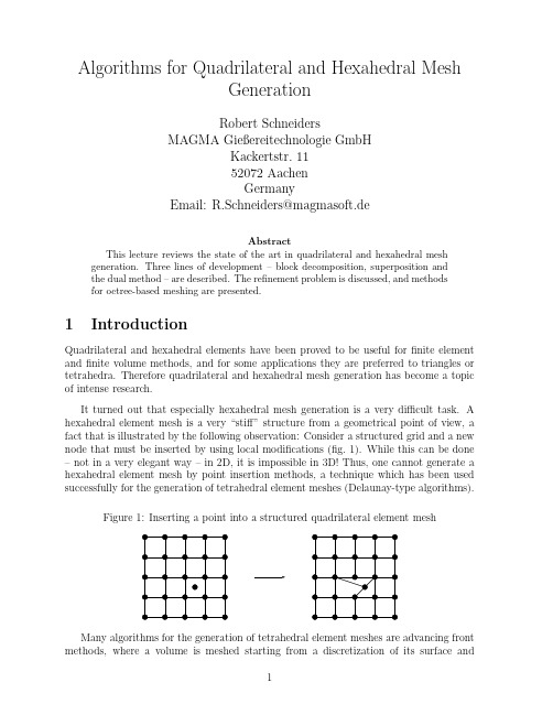
Algorithms for Quadrilateral and Hexahedral MeshGenerationRobert SchneidersMAGMA Gießereitechnologie GmbHKackertstr.1152072AachenGermanyEmail:R.Schneiders@magmasoft.deAbstractThis lecture reviews the state of the art in quadrilateral and hexahedral mesh generation.Three lines of development–block decomposition,superposition andthe dual method–are described.The refinement problem is discussed,and methodsfor octree-based meshing are presented.1IntroductionQuadrilateral and hexahedral elements have been proved to be useful forfinite element andfinite volume methods,and for some applications they are preferred to triangles or tetrahedra.Therefore quadrilateral and hexahedral mesh generation has become a topic of intense research.It turned out that especially hexahedral mesh generation is a very difficult task.A hexahedral element mesh is a very“stiff”structure from a geometrical point of view,a fact that is illustrated by the following observation:Consider a structured grid and a new node that must be inserted by using local modifications(fig.1).While this can be done –not in a very elegant way–in2D,it is impossible in3D!Thus,one cannot generate a hexahedral element mesh by point insertion methods,a technique which has been used successfully for the generation of tetrahedral element meshes(Delaunay-type algorithms).Figure1:Inserting a point into a structured quadrilateral element meshMany algorithms for the generation of tetrahedral element meshes are advancing front methods,where a volume is meshed starting from a discretization of its surface and1building the volume mesh layer by layer.It is very difficult to use this idea for hex meshing,even for very simple structures!Fig.2shows a pyramid whose basic square has been split into four and whose triangles have been split into three quadrilateral faces each.It has been shown that a hexahedral element mesh exists whose surface matches the given surface mesh exactly[Mitchell1996],but all known solutions[Carbonera]have degenerated or zero-volume elements.Figure2:Surface mesh for a pyramidThe failure of point-insertion and advancing-front type algorithms severely limits the number of approaches to deal with the hex meshing problem.Most algorithms can be classified either as block-decomposition,superposition or dual methods,which will be presented in section2,section3and section4.Adaptive mesh generation is more difficult than for triangular and tetrahedral meshes. Fig.3shows an example:The mesh infig.3a has been derived from a structured quadri-lateral mesh by recursively splitting elements.In order to get rid of the hanging nodes, neighboring elements are split to create a conformal transition to the coarse part of the mesh(fig.3b).This probleem is equivalent to the generation of quadrilateral/hexahedral meshes from a quadtree/octree structure.Figure3:Quadrilateral mesh refinementa)b)Fig.4shows a simple example for the3D case(motivated by octree-based meshing) where thefine region seems to be connected to the coarse in a reasonable manner.Un-fortunately,the solution is not valid!This can be concluded from the following relation between the number of elements H,the number of internal faces F i and the number of boundary faces F b of a hexahedral mesh:6·H=2·F i+F b(1)Figure4:Non-convex transitioningTherefore,for any hexahedral mesh the number F b of boundary faces must be even. This does not hold for the example offig.4,so that no hexahedral mesh for that surface mesh exists,and the transitioning is not valid.The mesh refinement problem will be discussed in detail in section5,where we will also solve the problem presented infig.4.Much of the research work has been presented in the Numerical Grid Generation in Computational Fluid Dynamics and in the Mesh Generation Roundtable and Conference conference series,and detailed information can be found in the proceedings.The proceed-ings of the latter one are available online at the Meshing Research Corner[Owen1996], a large database with literature on mesh generation maintained at Carnegie Mellon Uni-versity by S.Owen.Another valuable source of online information is the web page Mesh Generation and Grid Generation on the Web[Schneiders1996d]which provides links to software,literature and homepages of research groups and individuals.An overview on the state of the art in mesh generation is given in the Handbook of Grid Generation [Thompson1999],which has been compiled by the International Society on Grid Gener-ation().2Block-Decomposition MethodsIn the early years of thefinite element method,hexahedral element meshes were the meshes of choice.The geometries considered at that time were not very complex(beams, plates),and a hexahedral element mesh could be generated with less effort than a tet mesh(graphics workstations were not available at that time).Meshes were generated by using mapped meshing methods:A mesh defined on the unit cube is transformed onto the desired geometryΩwith the help of a mapping F:[0,1]3→Ω.This method can generate structured grids for cube-like geometries(Fig.5).Figure5:Mapped meshingThe mapping F can be specified explicitly(isoparametric or conformal mapping)or implicitly(solution of an ellpitic or hyperbolic partial differential equation).The problem offinding a suitable mapping F has been the object of major research efforts in recent years,and an overview is given elsewhere in this volume.A summary of the results can be found in the books of Thompson[Thompson1985]and Knupp[Knupp1995].If the geometry to be meshed is too complicated or has reentrant edges,meshes gen-erated by mapped meshing methods usually have poorly-shaped elements and cannot be used for numerical simulations.In this case,a preprocessing step is required:The ge-ometry is interactively partitioned into blocks which are meshed separately(the meshes at joint interfaces must match,a problem considered in[Tam and Armstrong1993]and [M¨u ller-Hannemann1995]).These multiblock-type methods are state of the art in univer-sity and industrial codes.Fig.6shows an example mesh that was generated with Fluent Inc.’s GEOMESH1preprocessor.Figure6:Multiblock-structured meshIn principle,most geometries can be meshed in this way.However,there is a limita-tion in practice:The construction of the multiblock decomposition,which must be done interactively by the engineer.For complex geometries,e.g.aflowfield around an airplane or a complicated casting geometry,this task can take weeks or even months to complete. This severely prolongs the simulation turnaround time and limits the acceptance of nu-merical simulations(a recent study suggests that in order to obtain a24-hour simulation turnaround time,the time spent for mesh generation has to be cut to at most one hour).One way to deal with that problem is to develop solvers based on unstructured tetra-hedral element meshes.In the eighties,powerful automatic tethrahedral element meshers have been developed for that purpose(they are described elsewhere in this volume).Thefirst attempt to develop a truly automated hex mesher was undertaken by thefinite element modeling group at Queens University in Belfast(C.Armstrong).Their strategy is to automate the block decomposition process.The starting point is the derivation of a simplified geometrical representation of the geometry,the medial axis in2D and the medial surface in3D.In the following we will explain the idea(see [Price,Armstrong,Sabin1995]and[Price and Armstrong1997]for the details).We start with a discussion of the2D algorithm.Consider a domain A for which we want tofind a partition into subdomains A i.We define the medial axis or skeleton of A as follows:For each point P∈A,the touching circle U r(P)is the largest circle around P which is fully contained in A.The medial axis M(A)is the set of all point P whose touching circles touch the boundaryδA of A more than once.Figure7:Medial axis and domain decompositionThe medial axis consists of nodes and edges and can be viewed as a graph.An example is shown infig.7:Two circles touch the boundary of A exactly twice;the respective midpoints fall on edges of the medial axis.A third circle has three common points with δA,the midpoint is a branch point(node)of the medial axis.The medial axis is a unique description of A:A is the union of all touching circles U r(P),P∈M(A).The medial axis is a representation of the topology of the domain and can thus serve as a starting point for a block decomposition(fig.7and8).For each node of M(A)a subdomain is defined,its boundary consisting of the bisectors of the adja-cent edges and parts ofδA(a modified procedure is used if non-convex parts ofδA come into play[Price,Armstrong,Sabin1995]).The resulting decompostion of A con-sists of n−polygons,n≥3,whose interior angle are smaller than180o.A polygon is then split up by using the midpoint subdivision technique[Tam and Armstrong1993], [Blacker and Stephenson1991]:It’s centroid is connected to the midpoints of it’s edges, the resulting tesselation consists of convex quadrilaterals.Fig.8shows the multiblock de-compostion and the resulting mesh which can be generated by applying mapped meshing to the faces.It remains to explain how to construct the medial axis.This is done by using a Delaunay technique(fig.9a):The boundaryδA of the domain A is approximated by a polygon p,and the constrained Delaunay triangulation(CDT)of p is computed.One gets an approximation to the medial axis by connection of the circumcircles of the Delaunay triangulation(the approximation is a subset of the Voronoi diagram of p).By refining the discretization p ofδA and applying this procedure one gets a series of approximations that converges to the medial axis(fig.9b).Consider a triangle of the CDT to p:Part of it’s circumcircle overlaps the complement of A.The overlap for theFigure8:Multiblock-decomposition and resulting meshcircumcircle of the respective triangle of the refined polygon’s CDT is significantly smaller. If the edge lengths of p tend to zero,the circumcircles converge to circles contained in A which touchδA at least twice.Their midpoints belong to the medial axis.Figure9:Approximating the medial axisa)b)In three dimensions,the automization of the multiblock decomposition is found by using the medial surface.The medial surface is a straightforward generalization of the medial axis and is defined as follows:Consider a point P in the object A and let U r(P) the maximum sphere centered in P that is contained in A.The medial surface is defined as the set of all points P for which U r(P)touches the object boundaryδA more than once.P lies on–a face of the medial surface,if U r(P)touchesδA twice–an edge of the medial surface,if U r(P)touchesδA three times–a node of the medial surface,if U r(P)touchesδA four times or more.The medial surface is a simplified description of the object(again,A is the union of the touching spheres U r(P)for all points P on the medial surface).The medial surface preserves the topology information and can therefore be used forfinding the multiblock decomposition.Armstrong’s algorithm for hexahedral element mesh generation follows the line of the 2D algorithm(fig.10).Thefirst step is the construction of the medial surface with the help of a constrained Delaunay triangulation(Shewchuk[Shewchuk1998]shows how to construct a surface triangulation for which a constrained Delaunay triangulation ex-ists).The medial surface is then used to decompose the object into simple subvolumes. This is the crucial step of the algorithm,and it is much more complex than in the two-dimensional case.A number of different cases must be considered,especially if non-convexFigure10:Medial-surface algorithm for the generation of hexahedral element meshes(a) medial surface(a) edge primitives(c) vertex primitives(d) face primitives(e) final meshedges are involved;they will not be discussed here,the interested reader is referred to [Price and Armstrong1997]for the details.Figure11:Meshable primitives(selection)Armstrong identifies13polyhedra an object is decomposed to(fig.11shows a selec-tion).These meshable primitives have convex edges,and each node is adjacent to exactly three edges.The midpoint subdivision technique[Tam and Armstrong1993]can there-fore be used to decompose the object into hexahedra:The midpoints of the edges are connected to the midpoints of the faces(fig.12).Then both the edge and face midpoints are connected to the center of the object,and the resulting decompostion consists of valid hexahedral elements.Fig.13shows a mesh generated for a geometry with a non-convex edge.The example highlights the strength of the method:The mesh is well aligned to the geometry,it is a “nice”mesh–an engineer would try to create a mesh like this with an interactive tool.Figure12:Volume decomposition by midpoint subdivision.Figure13:Medial surface and mesh for a mechanical partThe medial surface technique tries to emulate the multiblock decomposition done by the engineer“by hand”.This leads to the generation of quality meshes,but there are some inherent problems:Namely,it does not answer the question whether a good block decomposition exists,which may not be the case if the geometry to be meshed has small features.Another problem is that the medial surface is an unstable entity:Small changes in the object can cause big changes in the medial surface and the generated mesh.Nevertheless,the medial surface is extremly useful for engineering analysis:It can be used for geometry idealization and small feature removal,which simplifies the medial surface,enhances the stability of the algorithm and leads to better block decompositions. The method delivers relatively coarse meshes that are well aligned to the geometry,a highly desirable property especially in computational mechanics.It is natural that an approach to high-quality mesh generation leads to a very complex algorithm,but the problems are likely to be solved.Two other hex meshing algorithms based on the medial surface are known in the litera-ture.Holmes[Holmes1995]uses the medial surface concept to develop meshing templates for simple subvolumes.Chen[Turkkiyah1995]generates a quadrilateral element mesh on the medial surface which is then extended to the volume.3Superposition MethodsThe acronym superposition methods refers to a class of meshing algorithms that use the same basic strategy.All these algorithms start with a mesh that can be more or less easilygenerated and covers a sufficiently large domain around the object,which is then adapted to the object boundary.The approach is very pragmatic,but the resulting algorithms are very robust,and there are several promising variants.Since we have actively participated in this research,we will concentrate on a descrip-tion of our own work,the grid based algorithm[Schneiders1996a].Fig.14shows the2D variant:A sufficiently large region around the object is covered by a structured grid.The cell size h of the grid can be chosen arbitrarily,but should be smaller than the smallest feature of the object.It remains to adapt the grid to the object boundary–the most difficult part of the algorithm.Figure14:2D-grid based algorithma)b)c)According to[Schneiders1996a],all elements outside the object or too close to the object boundary are removed from the mesh,with the remaining cells defining the initial mesh(fig.14a,note that the distance between the initial mesh and the boundary is approximately h).The region between the object boundary and the initial mesh is then meshed with the isomorphism technique:The boundary of the initial mesh is a polygon, and for each polygon node,a node on the object boundary is defined(fig.14b).Care must be taken that characteristic points of the object boundary are matched in this step, a problem that is not too difficult to solve in2D.By connecting polygon nodes to their respective nodes on the object boundary,one gets a quadrilateral element mesh in the boundary region(fig.14c).The“principal axis”of the mesh depends on the structure of the initial mesh,and in the grid based algorithm the element layers are parallel to one of the coordinate axis. Consequently,the resulting mesh(fig.14)has a regular structure in the object interior and near boundaries that are parallel to the coordinate axis,irregular nodes can be found in regions close to other parts of the boundary.This is typical for a grid based algorithm, but can be avoided by choosing a different type of initial mesh.The only input parameter for the grid based algorithm is the cell size h.In case of failure,it is therefore possible to restart the algorithm with a different choice of h,a fact that greatly enhances the robustness of the algorithm.Another way to adapt the initial mesh to the boundary,the projection method,was proposed in[Taghavi1994]and[Ives1995].The starting point is the construction of a structured grid that covers the object(fig.15a),but in contrast to the grid based algorithm,all cells remain in place.Mesh nodes are moved onto the characteristic points of the object and then onto the object edges,so that the object boundary is fully covered by mesh edges(fig.15b).Degenerate elements may be constructed in this step,but disappear after buffer layers have been inserted at the object boundary(fig.15c,the mesh is then optimized by Laplacian smoothing).Figure15:Grid based algorithm–boundary adaption by projection techniquea)b)c)The projection method allows the meshing objects with internal faces;the resulting meshes are similar to those generated with the isomorphism techniques,although there tend to be high aspect ratio elements at smaller features of the object.In contrast to the isomorphism technique,the mesh is adapted to the object boundary before inserting the buffer layer.Figure16:Grid based algorithm–boundary adaption by cell splitting technique a)b)c)Only recently,a third method has been proposed[Dhondt1999].With this approach,only nodes that are very closed to the bounary are projected onto it.Grid cells that are crossed ty a boundary edge are split(fig.16b).Midpoint subdivision is used to split the 3-and5-noded faces(fig.16c).Dangling nodes are removed by propagating the split throughout the mesh.The superposition principle generalizes for the3D case.The idea of the grid based algorithm is shown for a simple geometry,a pyramid(1quadrilateral,4triangular faces,fig.17).The whole domain is covered with a structured uniform grid with cell size h.In order to adapt the grid to the boundary,all cells outside the object,that intersect the object boundary or are closer the0.5·h to the boundary are removed from the grid.The remaining set of cells is called the initial mesh(fig.17a).Figure17:Initial mesh and isomorphic mesh on the boundarya)b)The isomorphism technique[Schneiders1996a]is used to adapt the initial mesh to the boundary,a step that poses many more problems in3D than in2D.The technique is based on the observation that the boundary of the initial mesh is an unstructured mesh M of quadrilateral elements in3D.An isomorphic mesh M′is generated on the boundary:For each node of v∈M a node v′∈M′is defined on the object boundary,and for each edge (v,w)∈M an edge(v′,w′)∈M′is defined.It follows that for each quadrilateral f∈M of the initial mesh’s surface there is exactly one face f′∈M′on the object boundary. Fig.17b shows the isomorphic mesh for the initial mesh offig.17b.Fig.18shows the situation in detail:The quadrilateral face(A,B,C,D)∈M cor-responds to the face(a,b,c,d)∈M′.The nodes A,B,C,D,a,b,c,d define a hexahedral element in the boundary region!This step can be carried out for all pairs of faces,and the boundary region can be meshed with hexahedral elements in this way.The crucial step in the algorithm is the generation of a good quality mesh M′on the object boundary:All object edges must be matched by a sequence of mesh edges, and the shapes of the faces f′∈M′must be non-degenerate.If the surface mesh does not meet these requirements,the resulting volume mesh does not represent the volume well or has degenerate elements.Fulfilling this requirement is a non-trivial task,also the implementation becomes a problem(codes based on superposition techniques usually have more than100.000lines of code).We will not describe the process in detail,but some important steps will be discussed for the example shown infigs.19-24.Fig.19a shows the initial mesh for another geometry that does not look very compli-Figure 18:Construction of hexahedral elements in the boundaryregion a bc da’b’c’d’cated but nevertheless is difficult to mesh.The first step of the algorithm is to define thecoordinates of the nodes of the isomorphic mesh.Therefore,normals are defined for thenodes on the surface of the initial mesh by averaging the normals N f of the n adjacentfaces f (cf.fig.19b):N v =1Figure20:Isomorphic surface mesha)b)nodes in space.This allows the optimization of the surface mesh by moving the nodes v′to appropriate positions(fig.20b shows that the quality of the surface mesh can be improved significantly).A Laplacian smoothing is applied to the nodes of the surfacemesh:The new position x newi of a node v′is calculated as the average of the midpointsS k of the N adjacent faces.x new i =1from the edge capturing process if three nodes of a face arefixed to the same characteristic edge.This cannot be avoided if the object edges are not aligned to the“principal axes”of the mesh(cf.fig.21).There are two ways to deal with the problem.First,the boundary region isfilled with a hexahedral element mesh.Due to the meshing procedure,there are two rows of elements adjacent to a convex edge(fig.22a).If the solid angle alongside the edge is sufficiently smaller than180o,the mesh quality can be improved by inserting an additional row of elements,followed by a local resmoothing. At object vertices where three convex edges meet,one additional element is inserted.Figure22:Inserting additional elements at sharp convex edgesa)b)Fig.24a shows the resulting mesh after the application of the optimization step(note that many degeneracies have been removed).The remaining degenerate elements are removed by a splitting procedure.Figure23:Splitting degenerated elementsa)b)Figure24:Removing degenerated elementsa)b)Fig.23shows the situation:Three points of a face have beenfixed to a characteristic edge,the node P is“free”.This face is split up into three quadrilaterals in a way that the flat angle is removed(fig.23b).The adjacent element can be split in a similar way into four hexahedral elements.In order to maintain the conformity of the mesh,the neighborelements must be split up also;it is,however,important that only neighbor elements adjacent to P must be refined,the initial mesh remains unchanged.Fig.24b shows the resulting mesh.Note that the surface mesh is no longer isomorphic to the initial mesh(fig.19a),since removing the degenerated elements has had an effect on the topology(the mesh infig.20b is isomorphic to the initial mesh).The mesh has a regular structure at faces and edges that are parallel to one of the coordinate axes. The mesh is unstructured at edges whose adjacent edges include a“flat”angle and where degenerate elements had to be removed by the splitting operation.Fig.25shows another mesh for a mechanical part.Figure25:Mesh for a mechanical partThe grid based algorithm is only one out of many possible ways use the superposition principle.One can take an arbitrary unstructured hexahedral mesh as a starting point–the adaptation to the boundary is general,no special algorithm is needed.Fig.26shows an example where a non-uniform initial mesh has been generated and adapted to the object boundary by the isomorphism technique.Figure26:Octree-based initial mesh and isomorphic surface meshThis makes the superposition principle a powerful tool for hex meshing.Several vari-ants of the idea have been proposed.Fig.27shows a hexahedral mesh generated to model a part of a turbine.For the smallfeature,a thin initial mesh has been generated.The mesh was adapted to the boundaryby using the method proposed in[Dhondt1999].Figure27:Mesh for a part of a turbineA weak point of the grid based method is the fact that the elements are nearly equal-sized.This can cause problems,since the element size h must be chosen according tothe smallest feature of the object–a mesh with an inacceptable number of elementsmay result.The natural way to overcome this drawback is to choose an octree-basedstructure as an initial mesh.NUMECA’s new unstructured grid generator IGG/Hexa2[Tchon1997]uses this technique,fig.28shows an example of how it works.The initialmesh has hanging nodes,and so does the the mesh on the boundary.Figure28:Fig.29shows a mesh generated with IGG/Hexa around a generic business jet con-figuration.The mesh was generated automatically from an initial cube surrounding thegeometry.Anisotropic adaptation to the geometry is performed in a fully automated waywith a criteria based on normal variation of the surface triangles intersected by the cell.Three layers of high aspect ratio cells are introduced close to the wall.Figure29:Mesh around a jet configurationThe mesh infig.29has hanging nodes in the interior,which is of disadvantage for some applications.In this case,one can use an octree structure as a starting point,remove thehanging nodes from the octree and use this as an initial mesh.This has been proposed in [Schneiders1998],fig.30shows a shows part of a mesh that has been generated for thesimulation offlow around a car.This technique will be discussed in detail in chapter5ofthis lecture.Figure30:Hexahedral element mesh for the simulation offlow around a carThe grid-and octree-based algorithms presented here prove that the superpositionprinciple is a very useful algorithmic tool to deal with the hex meshing problem.Most commercial hexahedral mesh generators are of this type..The algorithms mentioned here are not the only variants of the strategy,combinations with the other methods seem promising.Further research may reveal the full potential of superposition methods.4The spatial twist continuumThe techniques presented so far can also be used for the generation of tetrahedral ele-ment meshes.In contrast to that,the spatial twist continuum is a unique concept for quadrilateral and hexahedral element mesh generation.Many of the results presented here were achieved by the CUBIT team,a joint re-search group at SANDIA National Laboratories and Brigham Young University that is in quadrilateral and hexahedral element meshing research since the beginning of the 90’s.The group is working on algorithms that generate a mesh starting from discretiza-tion of the object surface into quadrilaterals.As part of their research,the paving [Blacker and Stephenson1991]and plastering[Blacker1993]advancing-front type mesh generators have been developed.These algorithms will be described in chapter6,here we will present other results.Def.1Given an unstructured quadrilateral element mesh M=(V,E,F),the spatial twist continuum(STC)[Murdock et al.1997]M′=(V′,E′,F′)is defined as follows:–For each face f∈F,the midpoint v′is a node of V′.–For each edge e∈E we define an edge e′=(v′1,v′2)∈E′where v′1and v′2are the midpoints of the two quadrilaterals that share e.For each node v∈V a face f′∈F′is defined by the midpoints of the adjacent quadrilaterals.The STC is the combinatorial dual[Preparata and Shamos1985]of the quadrilateral mesh,just as a Delaunay triangulation and it’s corresponding Voronoi dia-gram are combinatorical dual.Figure31:Quadrilateral mesh and spatial twist continuumFig.31shows a quadrilateral mesh(straight lines)and the STC(dotted lines).The edges of the STC are displayed not as straight lines but as curves.This allows the recognition of chords,a very important structure:One can start at a node,follow an edge e1to the next node,then choose the edge e2“straight ahead”that is not adjacent to e1,continue to the next edge e3and so on.The sequence e1,e2,...forms a chord (displayed as a smooth curve infig.31).Chords can be closed or open curves and can have self-intersections,and no more than2chords are allowed to intersect at one point.。
icem-cfd 四面体网格模块tetra介绍

z Choose Solver Input
− select desired domain(s) and click Done
z Options are specific to solver
Tetra 29
2 July 2008
Tetra 示例实践3
Tetra 19
2 July 2008
机翼例子:网格参数
z 细化
− integer, number of cells in 360 degrees of an arc
Tetra 20
2 July 2008
自然尺寸和细化
z Example, two rods in close proximity z 网格参数::
2 July 2008
所有程序综述
z 创建或读入几何图形 z 将实体分配到几何图形数据库 z 定义网格全局尺寸和在所选实体上的尺寸 z 产生网格 z 提高网格质量(光滑,等) z 输出到分析软件
Tetra 4
2 July 2008
Tetra的几何图形
z 需要封闭的曲面模型
− 将曲面显示为实体 • 查找丢失的表面 • 查找洞或缺口
2 July 2008
机翼例子:设置
z 创建族
− 机翼 − 入口 − 出口 − Symm − 壁面
z 材料点
− live
Tetra 18
2 July 2008
机翼例子:网格参数
z Ref. size and max. size explained earlier z 自然尺寸
− factor times ref. size − represents a ‘minimum’ size
认识网格3:选择合适的网格类型

认识网格3:选择合适的网格类型学习有限元分析初期一般比较强调网格的重要性,这个阶段大家会了解到各种各样的网格(单元)类型,如质点,梁,三角形/四面体,四边形/六面体等等,每种网格有其各自特点应用于不同的场合。
其中,四面体和六面体的选择问题一直是大家争议的话题,因此本文主要从个人角度给出一些建议,希望对大家有所帮助。
易用性早期分析工程师受限于计算机的求解能力,会花大部分时间进行几何特征的简化以及模型的切分来得到完善的六面体网格。
现在普通的个人笔记本也能比较轻松地完成几十万节点的计算,再加上有限元分析技术在工程领域的推广需要压缩前处理工作的占比使其看起来更加便于使用,因此长期被打入冷宫的四面体网格又重新焕发了生机。
这个时候大家更加注重网格的易用性,个人主要从两个角度进行说明:复杂特征的适应性,局部加密的便捷性。
复杂特征的适应性如图所示基本几何体使用六面体进行划分能够一键生成,但是如果加上螺栓孔,整体的映射路径被打断,这个时候就需要进行切割使得各部分可以映射,并控制相应面网格质量才能得到质量较高的六面体网格:当更多的特征考虑进去后,需要进行更多的切割以及面网格控制才能得到高质量的六面体网格:然而实际工程模型远远比上述复杂,如果前期不通过大量的经验对模型进行合理地简化,基本上很难使用六面体进行网格划分,这个时候四面体的优势就比较明显:由于使用四面体进行网格划分不需要像六面体那样规则,因此对于复杂特征能够在不进行过多人为控制的情况下更好的适应,这一点上四面体具有绝对的优势。
局部加密的便捷性在进行应力分析时,局部应力集中比较明显的区域需要进行网格加密才能较好地模拟应力变化趋势。
常见的四边形局部加密有以下两类(偏置和切分):如果将其扩展到六面体上如下:显然,使用偏置类进行加密虽然能让单元尺寸渐进变化,但是随着加密程度的增加,会出现大量细长的实体单元,使用1:2等切分方式虽然能够避免细长单元,但是需要大量的切割工作,并且两种加密方式都对几何模型的规正性要求极高,而使用四面体进行局部加密相对就容易得多:可以看到,四面体对于需要加密的几何特征或者指定的局部加密区域都能较方便的进行过渡,并且不受模型复杂程度的限制,因此这一点上,四面体相比于六面体优势也很明显。
2024版FEMAP培训教程1

03
网格划分与优化策略
网格划分原则及技巧分享
遵循几何特征
根据模型的几何形状、尺寸和特 征进行网格划分,确保网格能够
准确反映模型的细节。
均匀性原则
尽量保持网格的均匀性,避免出 现过大或过小的网格,以提高计 算精度和稳定性。
问题解答和互动交流环节
针对学员在练习过程 中遇到的问题,进行 解答和指导。
通过讨论和互动,加 深对有限元分析方法 和应用的理解。
鼓励学员之间的互动 交流,分享各自的经 验和心得。
THANKS
感谢观看
FEMAP培训教程1
目录
• FEMAP软件简介与安装 • 模型建立基础 • 网格划分与优化策略 • 求解器设置与运算过程监控 • 后处理功能深入挖掘 • 实际应用案例分析与讨论
01
FEMAP软件简介与安装
FEMAP软件概述
FEMAP是一款广泛应用于有限元分析的软件,具有强大的前处理和后处理功能。
支持多种CAD软件格式(如 SolidWorks、CATIA、AutoCAD等) 的导入,实现与外部CAD软件的无缝 对接。
材料属性设置与分配
01
02
03
材料库管理
内置丰富的材料库,用户 可自定义材料属性并添加 到材料库中,方便后续调 用。
材料属性分配
将材料属性分配给几何模 型中的各个部分,确保分 析结果的准确性。
进度条
部分软件提供进度条果文件类型
01
了解并掌握各种结果文件的输出方式和查看方法,如文本文件、
二进制文件等。
后处理软件
02
利用后处理软件查看和分析结果文件,如云图、等值线图等。
Gambit学习总结

容值:是指操作新老几何之间的最大缝合距离,可分为自动和手动,自动是指按照系统默认值进行操作,手动则可指定缝合距离(默认情况下是10-3)。
平滑示例:
修复示例:
3.6虚几何操作
反之可以利用Disconnect功能将连接好的实体断开。
3.4分割
分割操作可以利用一个实体将另外一个实体分割成一个或多个对象。以下图为例说明面的分割,蓝框表示图形A,绿框表示图形B。
以B来分割A,则出现以下两个面:
以A来分割B,则出现以下两个面:
如果选择互相分割,则会出现以下三个面:性是一个非常重要的概念,它可以使流体从一个面(或体)传递到另一个面(或体),但这两个面(或体)必须是连接的或者是非形定义的。
形网格:点在体的交界面处共享;
非形网格:点在体的交界面处不共享。
形网格非形网格
点、线、面都可以连接,该操作将消除所有重复的实体并重新连接拓扑结构,但只有实体才会被连接,在连接的同时,现有网格会被保存。
合并:将两个体合并成一个实体或虚体;
分割:将一个体分割成两个实体或虚体;
连接:将两个体连接成一个虚体。
3.7Unite、Merge和Connect的比较
Unite(Real):面必须有匹配的切线;
Unite(Virtual):空隙和重叠是允许的,但不能连结边;
Merge:可以在实体或者虚体上操作,结果永远是虚体,面与面之间必须共享一条边,但不必相切:
Reset:删除所有的网格和几何;
Reset mesh:删除网格但保留几何。
2
Gambit的菜单栏主要包括三个部分,分别是文件菜单、编辑菜单和求解器菜单。
FEMAP培训教程1
有限元预备知识
(3)弹性极限:材料在外力作用下将产生变形,但是去除外力后仍能恢复原 状的能力称为弹性。金属材料能保持弹性变形的最大应力即为弹性极限,相应 于拉伸试验曲线图中的e点,以σe表示,单位为兆帕(MPa):σe=Pe/Fo 式中 Pe为保持弹性时的最大外力 。 (4)弹性模数:这是材料在弹性极限范围内的应力σ与应变δ(与应力相对应 的单位变形量)之比,用E表示,单位兆帕(MPa):E=σ/δ=tgα 式中α为拉伸 试验曲线上o-e线与水平轴o-x的夹角。反映金属材料刚性的指标。 (5)疲劳强度极限:金属材料在长期的反复应力作用或交变应力作用下(应 力一般均小于屈服极限强度σs),未经显著变形就发生断裂的现象称为疲劳 破坏或疲劳断裂,这是由于多种原因使得零件表面的局部造成大于σs甚至大 于σb的应力(应力集中),使该局部发生塑性变形或微裂纹,随着反复交变 应力作用次数的增加,使裂纹逐渐扩展加深(裂纹尖端处应力集中)导致该局 部处承受应力的实际截面积减小,直至局部应力大于σb而产生断裂。
21
有限元预备知识:有限元分析及应用
第二类问题,通常可以建立它们应遵循的基本方程,即微分方程 和相应的边界条件。例如弹性力学问题,热传导问题,电磁场问 题等。由于建立基本方程所研究的对象通常是无限小的单元,这 类问题称为连续系统,或场问题。 尽管已经建立了连续系统的基 本方程,由于边界条件的限制 ,通常只能得到少数简单问题 的精确解答。对于许多实际的 工程问题,还无法给出精确的 解答,例如图示V6引擎在工作 中的温度分布。为解决这个困 难,工程师们和数学家们提出 了许多近似方法。
有限元法的力学基础
• • • 材料力学与弹性力学的比较 弹性力学的基本方程 虚功原理及极小
18
有限元预备知识:有限元分析及应用
ANSA初级培训_六面体网格
CAE咨询,找有限元在线! ---因为专注,所以卓越!
400-639-6699
ANSA中六面体的生成步骤与方法
ANSA生成六面体共有六种方法,:
方法一:
CAE咨询,找有限元在线! ---因为专注,所以卓越!
400-639-6699
ANSA中划分一般复杂几何模型六面体网格
ANSA中检查六面体单元质量常用标准
1. 2. 3. 4. 5. 6.
边长比 ASPECT RATIO 偏斜 SKEWNESS 翘曲 WARPING 雅可比 JACOBIAN 边长范围 LENGTH 内角角度 ANGLE
等等……
CAE咨询,找有限元在线! ---因为专注,所以卓越!
ANSA中划分一般复杂几何模型六面体网格
ANSA中几何模型的六面体分块及拉伸
分块完成后,先要给几何分配节点,厚度方向及筋板特征的节点;
分配完节点后,按照从复杂特征到简单特征的准则依次拉伸。
CAE咨询,找有限元在线! ---因为专注,所以卓越!
400-639-6699
400-639-6699
ANSA中划分一般复杂几何模型六面体网格
ANSA中几何模型的六面体分块及拉伸
根据MAP准则对几何进行分块,分块先从简单特征到复杂特征,按照次序依次切分。
CAE咨询,找有限元在线! ---因为专注,所以卓越!
400-639-6699
ANSA中划分一般复杂几何模型六面体网格
ANSA中六面体单元的检查与提高
在屏幕上双击off显示,不合格单元单独显示出来。使用 中的 自动
调整网格质量。
CAE咨询,找有限元在线! ---因为专注,所以卓越!
400-639-6699
四面体与六面体网格特征比较

四面体与六面体网格特征比较摘要:文章以一个轴承座零件为例,对轴承座零件分别进行了四面体和六面体网格划分,在此基础上,比较了四面体网格与六面体网格模型的特点,对有限元网格的划分具有一定的参照价值。
关键词:有限元;网格划分;模型比较作为有限元仿真的前处理技术,有限元的网格越来越受到分析工程师们的重视,有限元前处理(即CAD模型与网格划分)占CAE分析流程总时间的40%~45%左右,而计算结果的精确性却主要依赖网格的质量,所以有限元网格划分是进行有限元分析的重要步骤,它直接影响到后续工作的准确性。
六面体网格在计算精度、变形特性、划分网格数量、抗畸变程度及再划分次数等方面比三维四面体网格具有明显的优势,另外在某些情况下只能采用六面体单元进行有限元分析。
因此,六面体网格成为当今三维模型问题分析的首选网格。
然而,由于自动生成网格的需要,对于任意复杂的三维结构全部使用六面体网格划分网格是不现实的,因此,当计算任意形状的物体时,四面体是必不可少的工具。
本文利用有限元前处理软件HyperMesh,采取了两种方式分别对一个轴承座模型进行四面体和六面体的网格划分,比较了两种不同方式网格划分的特点。
1 四面体网格1.1 轴承座几何模型在PRO/E中建立轴承座的三维几何模型,并做了适当的简化处理,简化处理原则是对下一步的静强度计算没有太大影响,但是能有效减少网格单元数量,提高计算精度。
原模型只根据要求去除了支座底部的螺栓孔,保留了所有的圆角和筋等支撑,最大限度的不修改模型,简化后的几何模型如图1所示。
1.2 四面体网格的划分四节点四面体单元与十节点四面体单元是常见的两种四面体单元形式,与四节点单元相比而言,十节点四面体单元绝有较高的精度,但其单元函数相对复杂,生成数据后结构总数较多,计算效率低下,常应变四节点四面体单元虽然单元函数简单,结构自由度少,但是精度低,在HyperMesh中,有对微小曲面,狭窄倒圆角以及细长面的近似画法,对微小区域自动生成较小的网格单元,最大程度上保持了网格表面是三位模型表面的一致性,所以四面体单元比较适合对形状复杂的模型进行网格划分。
ICEM-CFD 四面体网格模块tetra介绍
z Use batch mode with ‘clean’ geometry
− no leakage expected
z 交互模式允许用户察看和修复问题
− 如果Tetra找到封闭体,Tetra就会显示曲面网格 − leakage indicated when a jagged line appears in display
Tetra 20
2 July 2008
感谢使用富静技术整理的学习资料,更多精彩请点击 /shop/view_shop.htm
自然尺寸和细化
z Example, two rods in close proximity z 网格参数::
− 在每个实体上指定当地尺寸 • This is ‘reference size’ times the ‘size’ specified on curves and surfaces
Tetra 3
2 July 2008
感谢使用富静技术整理的学习资料,更多精彩请点击 /shop/view_shop.htm
所有程序综述
z 创建或读入几何图形 z 将实体分配到几何图形数据库 z 定义网格全局尺寸和在所选实体上的尺寸 z 产生网格 z 提高网格质量(光滑,等) z 输出到分析软件
2 July 2008
感谢使用富静技术整理的学习资料,更多精彩请点击 /shop/view_shop.htm
使用点和曲线,例子
角上的点
Result with points and curves
边缘和曲面上的曲线
Tetra 7
Result without points and curves
球和立方体的例子
Femap图文教程

常用工具栏功能介绍
缩放、旋转和平移视图
撤销和重做
用于调整模型视图的显示方式。
选择和取消选择
撤销上一步操作或重做已撤销的 操作。
选择或取消选择模型中的元素。
新建、打开和保存文件
用于创建新文件、打开已有文件 和保存文件。
属性窗口
显示所选元素的属性信息,如几 何尺寸、材料属性等。
模型视图操作技巧
使用鼠标中键进行旋转和缩放视图。
05
在非关键区域采用较粗的网格划分,以提高计算效率。
06
注意网格的连续性和协调性,避免出现畸形网格或重叠网格。
04
Femap建模与网格划分
几何建模方法
01
02
03
直接建模
在Femap中直接创建几何 模型,利用基本图形元素 (如点、线、面)构建复 杂结构。
导入外部模型
支持多种CAD格式导入, 如STEP、IGES、 Parasolid等,实现与其他 CAD系统的无缝集成。
易用。
02
Femap界面与基本操作
界面组成与布局
菜单栏
包含文件、编辑、视图、工具、 窗口和帮助等菜单项,用于执 行各种命令。
状态栏
显示当前操作状态和相关提示 信息。
主窗口
显示模型、分析结果和其他主 要信息。
工具栏
提供常用命令的快捷按钮,方 便用户快速执行操作。
模型树
展示模型的层次结构,方便用 户管理和查看模型。
非
何在Femap中定义相关
线
材料参数。
性
介绍接触问题的基本原
理和求解方法,包括接
案 例
触对的定义、接触刚度
解
的设置等,并展示
析
Femap中的相关操作。
FEMAP培训教程1
23
有限元预备知识:有限元分析及应用
1-3 场问题的求解策略及方法
一、求解策略: • • 1、直接法:求解基本方程和相应定解条件的解; 2、间接法:基于变分原理,构造基本方程及相应定解条件的泛函形式 ,通过求解泛函的极值来获得原问题的近似解。即将微分形式转化与 其等价的泛函变分的积分形式; 二、求解方法: • • • • 1、解析或半解析法: 2、数值法: A)基于直接法的数值法,如差分法; B)基于间接法的数值法,如等效积分法(如里兹法)、有限元法等
28
有限元预备知识:有限元分析及应用
1-5 有限元法基本步骤
• 所研究问题的数学建模 (问题分析) • 结构离散 • 单元分析 (位移函数、单刚方程) • 整体分析与求解 (总刚方程与求解) • 结果分析及后处理
20
有限元预备知识:有限元分析及应用
1-1 工程和科学中典型问题
在工程技术领域内,经常会遇到两类典型的问题。第一类问题,可 以归结为有限个已知单元体的组合。例如,材料力学中的连续梁、建 筑结构框架和桁架结构。把这类问题称为离散系统。如左图所示平面 桁架结构,是由6个承受轴向力的“杆单元”组成。尽管离散系统是可 解的,但是求解右图这类复杂的离散系统,要依靠计算机技术。
有限元结果分析及可视化
• 有限元计算结果分类 • 有限元结果分析 • 有限元结果的可视化 常用有限元分析系统简介 • 有限元分析系统的基本组成 • 有限元分析系统的基本功能 • 常见商业化有限元分析系统
19
有限元预备知识:有限元分析及应用
绪论 • • • • • • • • • 1-1工程和科学中典型问题 1-2 场问题的一般描述 1-3 场问题的求解策略及求解方法比较 1-4 有限元法基本思想 1-5 有限元法的基本步骤 1-6 有限单元法的发展 1-7 有限单元法的基本内容 1-8 有限单元法的应用 1-9 有限元法的几个热点问题
有限元分析培训(第3讲-ANSYS-Workbench网格划分)

三 网格划分方法与参数设置
单元降阶设置
总体网格尺寸设置
三 网格划分方法与参数设置
关联中心和相关性的关系
三 网格划分方法与参数设置
o Active Assembly(激活装配体):初始种子放入末抑制部件。 o Full Assembly(全部装配体):初始种子放入所有装配部件,不管抑制部件的数量。 o Part(部件): 初始种子在网格划分时放入指定部件。
可以采用此种方式自动进行四面体(Patch Conforming)或扫掠网格划分。
如果几何体不规则,程序会自动产生四面体;如果几何体规则的话,就可以产
生六面体网格。
Body Operation
如果几何体不规则 可以通过切割和拓 扑重组成规则的几 何体组合,也可以 产生六面体网格。
三 网格划分方法与参数设置
域,可以自动判断区域并生成纯六面体网格,对不满足条件的 区域采用更好的非结构网格划分,多重区域网格划分和扫掠网 格划分相似,但更适合于用扫掠方法不能分解的几何体。
三 网格划分方法与参数设置
Automatic
在网格划分的方法中自动划分方法(Automatic)是最简单的划分方法,系统自动进
行网格的划分,但这是一种比较粗糙的方式,在实际运用中如不要求精确的解,
物理场
结构分析
Mechanical
电磁场分析
Electromagnetic
流体动力学分析 CFD
显式分析
Explicit
物理场网格默认选项
二次单元
Element Midside Nodes
是 Kept 是 Kept 否 Dropped 否 Dropped
关联中心
Relevance Center
hypermesh10.0基础培训day3
Copyright © 2009 Altair Engineering, Inc. Proprietary and Confidential. All rights reserved.
HyperMesh所提供的基本方法
• 体的四面体网格划分 (volume tetra mesher)
——对几何体直接进行四面体网格划分
Copyright © 2009 Altair Engineering, Inc. Proprietary and Confidential. All rights reserved.
标准四面体网格划分
Solid panel—drag
Copyright © 2009 Altair Engineering, Inc. Proprietary and Confidential. All rights reserved.
Solid panel—spin
• 通过旋转一组面单元来创建体单元。 • 恒定的横截面。 • 圆周型路径。 • 不能在一个没有孔的圆柱上使用该方法。
Do-it-yourself
Exercise(一): •完成Help里三维四面体网格划分实例, P90-94.
Copyright © 2009 Altair Engineering, Inc. Proprietary and Confidential. All rights reserved.
演示:四面体网格划分示例 模型:housing.hm
Copyright © 2009 Altair Engineering, Inc. Proprietary and Confidential. All rights reserved.
ICEM六面体网格划分ppt课件
– Curve 曲线 – Surface 曲面 – Volume 体
(material point, body)
Curve
Blocking – Vertex 顶点 – Edge 边 – Face 面 – Block 块
Vertex
Edge
Surfaces
Point
Face
9/9/05
Material point/body
扫描平面 Scan planes
– 作为质量直方图的辅助用来诊断坏网格的成因
– 使用Select按钮选择边, Scan planes垂直选定的边
– 或选择索引方向的代码
• #0 – i
• #1 – j
• #2 – k
• #3, 4, etc…
O-grids
Select 按钮用于选择 一条边 – scan plane 垂直于这个边
右击 Pre-mesh -> Scan planes 调出 scan plane 面板
9/9/05
ppt精选版
31
分块过程 – 输出网格
转变pre-mesh到永久网格 – 两种格式,取决于你使用的求解器 • 非结构 (Pre-mesh -> Convert to Unstruct Mesh) • 结构(File -> Blocking -> Save Multiblock Mesh) – 分块的改变不会再影响网格 – 此后网格可以通过Edit mesh 标签栏中的任何工具编辑 – 此后网格可以平滑
• 争取 < 45 度
–
检查网格质量
9/9/05
通过设置直方图,你可以显示指定质量范围内的网 格单元
ppt精选版
Femap_四面体单元网格质量
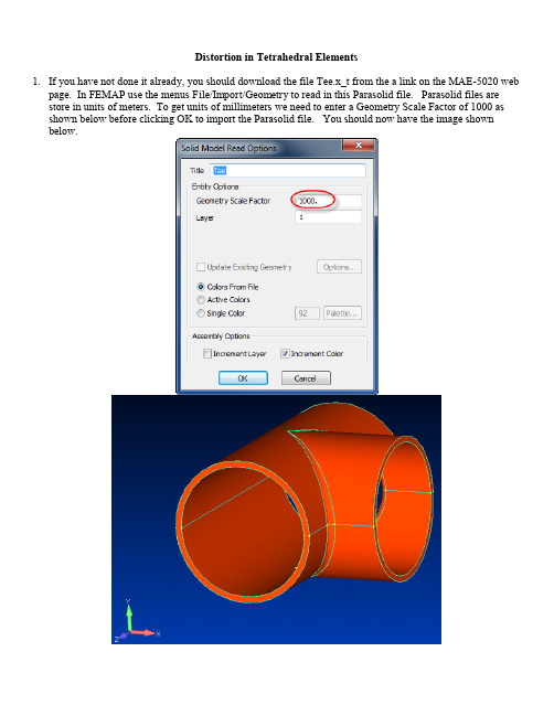
Distortion in Tetrahedral Elements1.If you have not done it already, you should download the file Tee.x_t from the a link on the MAE-5020 webpage. In FEMAP use the menus File/Import/Geometry to read in this Parasolid file. Parasolid files are store in units of meters. To get units of millimeters we need to enter a Geometry Scale Factor of 1000 as shown below before clicking OK to import the Parasolid file. You should now have the image shown below.2.Restrain all translations on the positive Z surface as shown below. Use the menusModel/Constraint/Surface to do this. You and just click OK on the first popup window for a constraint set name. In the next “Entity Selection” window select the surface shown below and click OK. In the “Create Constraints on Geometry” window, select the Pined radio button. Click OK and Cancel.3.Apply a 1000 mN/mm2 pressure on the positive X surface as shown below. Use the menusModel/Load/Surface, key in a Load Set name, select the surface and click OK, and in the popup window shown below, select Pressure and enter the pressure value. Click OK and Cancel.4.We will next set the mesh control to make a coarse mesh. From the menus select Mesh/Mesh Control/Sizeon Solids. Select the solid and click OK. In the popup window, make sure Tet Meshing is selected and key in an Element Size of 35. Click OK.5.Next, mesh the part by using the menus Mesh/Geometry/Solids. Since we have yet to define a material, thewindow below pops up. Key in the values shown which a representative for steel and click OK. In the Automesh Solids popup window you can just click OK using the default SOLID Property.6.You should now have the mesh shown below. We will turn off the solid to more clearly see the mesh. Aneasy way to do this is by clicking the icon. This toggles the geometry on and off.7.Notice that the edges of each tetrahedral element are straight. This is the default approach used by FEMAP.This overly coarse mesh does not well represent the geometry because of the straight edges. However, ifcurved edges were used, it creates elements with much more distortion (sufficient that an analysis couldfail). Let’s examine the distortion in the elements in this model. Select from the menusTools/Check/Element Quality. In the first popup window, click the Select All button to select all theelements and click OK. In the Check Element Distortions window, only select Aspect Ratio and Jacobian to be checked as shown below. This will make a list of elements with either Aspect ratios greater than 12 orJacobians greater than 0.85 to be displayed. We are also asking to create a group containing these elements.Click OK. A small portion of the display in the Messages window is shown below.Element Aspect Ratio Taper Alternate Taper Internal Angles Warping Nastran Warp Tet Collapse Jacobian Combined405 2.17881 0.86823 418 2.32891 0.85428 453 12.6647 0.66574 479 12.014 0.662248.The following information is from FEMAP’s documentation:“Valid elements prod uce Jacobian Distortion values between 0.0 and 1.0, where 0.0represents the "ideally shaped" element. Severely distorted elements whose Jacobiandeterminants are locally discontinuous or undefined are assigned a distortion value of 2. Ifany of your elements have a Jacobian Value of "2", the element is not valid (i.e., theelement is inside out, twisted, etc.) and should be fixed before analysis.”Thus, what FEMAP calls a Jacobian is not the same as the determinate of the Jacobian matrix as described in your text. However, per their guidelines, a 0 for distortion would be a perfectly shaped element and a 1.0 is on the outer limits of acceptance. If a value of 2.0 is obtained, the element is invalid! If you look through the message window, the worst distortion is 0.87346. Not a great element, but it will solve.To look at the elements in the group that was created, go to the Model Info window as shown below and click on the + in front of Groups, then right click on the group named “Distorted Elements” a nd selective Activate. Right click again on the group name and select “Show Active Group.”9.Your display will look something like the one below. If you rotate the model around, you will see theelements are getting very flat. Automatic meshing of tetrahedral elements can produce “flat” elements (i.e.they have very little volume).10.To displa y all the model instead of these “bad” elements, right click on the group name again and select“Show Full Model” as illustrated below.11.Proceed with a normal static solution as you have done before. You should not get any error messages.12.Click the icon and set the Contour parameter to Von Mises Stress and click OK. Click the andicons to display the deformed stress results.13.We will delete the results and the model. In the Model Info window, expand the Results + and right click onthe case and select Delete as shown below. In the next popup window, click the Go Fast button to delete the results.14.Now from the menus select Delete/Model/Mesh. In the popup window click the Select All button. In thenext popup window it asks if you want to delete unused properties and materials. Click NO.15. Because we turned off the geometry display, the screen looks funny. We need to turn the geometry backon. An easy way to do this is by clicking the icon.16.We will now mesh with more nodes. Select from the menus Mesh/Mesh Control/Size on Solid and selectthe part and click OK. In the popup window enter an Element Size of 10 and click OK.17.Next create a mesh on the part using the menus Mesh/Geometry/Solid. After making the mesh, your displayshould look like the one below. Notice how the mesh now more closely follows the curved geometry.18.Check the distortion in the elements again using the same parameters as used before. You will find that theJacobian values are reduced somewhat (0.873 to 0.786) but the aspect ratio has increased in some cases.You will find these elements located in corners of the joints and some mesh refinement in those areas might further reduce the aspect ratios.19.Look at the “worst” elements in the group we just created. In the Model Info window right click on thesecond group name to “Activate” and then “Show Active Group.” You will find these elements located in corners of the joints and some mesh refinement in those areas might further reduce the aspect ratios.20.Redisplay all the model by right clicking again on the second group name and selecting the “Show FullModel” item again. Next, solve this model. Display the Von Mises stress contour on the undeformedbody . Turn off the geometry display by click the icon. Turn off the nodes using the icon.When you have a fine mesh it helps to turn off the element edges. You can do this by holding down the left mouse button on the icon shown below and selecting the Filled Edges icon. Print this out and hand it in.。
四面体网格与六面体网格的比较

The advent of automatic tetrahedral (TET) and semi-automatic hexahedral (HEX) meshers in CAD and finite element systems started a recent controversy: should engineers dealing with designs that require solid finite elements model their designs with TET or HEX ele-ments?Solid regions containing thin-walled areas, concentrated loads, connection of assemblies with different materials and different types of elements stretch the capabilities of automatic meshing and the accuracy of the elements, regardless of the type. Such complex designs usually lead to problems with large numbers of DOF. In general, elements that meet impor-tant criteria such as shape functions contain-ing complete polynomials, having continuity across boundaries, and that satisfy the patch test, will converge. The real crux of the debate centers on the most efficient way to obtain accurate stresses for complex solid regions- rather than on the muddy waters of the relative merits of TET versus HEX ele-ments.HEX AND TET ARE BOTH BETTERAn article titled "A Performance Study of Tetrahedral Elements in 3D Finite Element Structural Analysis," by A.O. Cifuentes and A. Kalbag of IBM Research Division, Yorktown Heights, N.Y., in Finite Elements in Analysis and Desing in 1992, had an interesting conclu-sion. Its authors concluded, "…This study compares the performance of linear and quad-ratic tetrahedral elements and hexahedral ele-ments in various structural problems. The problems selected demonstrate the different types of behavior, namely bending, sheer, tor-sional and axial deformations. It was observed that the results obtained with quad-ratic tetrahedral elements and hexahedral were equivalent in terms of both accuracy and CPU time."The authors also noted that "For simple geometries, or for applications in which it is possible to build a mesh 'by hand,' analysts have relied heavily on the 8-node hexahedral element-commonly known as 'brick'…For more complex geometries, however, the ana-lyst must rely on automatic (or semi-automat-ic) mesh generators. In general, automatic mesh generators produce meshes of tetrahe-dral elements, rather than hexahedral ele-ments. The reason is that a general 3-D domain cannot always be decomposed into an assembly of bricks. However, it can always be represented as a collection of tetrahedral elements."Structural Research also ran similar studies comparing results of HEX vs. TET elements. The results of our studies were comparable to those of other reputable researches. With either type of element, the fewer the number of nodes, the lower the accuracy. The 4-node TET and the 8-node HEX approximate curved boundaries as straight lines and require many more elements to achieve convergence of curved boundary problems than do 10-node TET or 20-node HEX elements. However, it pays to remember that, because automatic HEX meshers contain so many limitations as to be semi-automatic at best, using HEX ele-ments may be more time-consuming than using 10-node TET elements, which take advantage of the speed of fully automatic meshing.HOW NEW TECHNOLOGY CHANGES THE DEBATENew technology, existing now, can reduce meshing time by starting with 4-node TET and 8-node HEX elements and then appreciably refining from both HEX and TET elementsautomatically- from 4- to 10-node TET and from 8- to 20-node HEX elements. Using the p-method, it can also increase the DOF of the 10-node TET so that it matches or exceeds the 20-node HEX in accuracy, without increas-ing computer resources. This, rather than the old HEX versus TET argument, is the real key to even more accurate and cost-effective analysis results.The new technology blends iterative and sparse matrix techniques to take lower order meshes, either 4-node TET or 8-node HEX, to form selective 10-node TET or 20-node HEX p-elements during the solution stage. Thus, element formulation and assembly takes place after the solid model has been meshed. The solution procedure can solve large numbers of DOF quickly, reducing computer time and stor-age space significantly. Because of this capa-bility, the new technology can take advantage of the fact that 10-node TET p-elements form system matrices with a smaller bandwidth than 20-node HEX elements, and can be solved faster for comparably accurate results. To avoid a new controversy, this time about h-or p-method meshing of HEX or TET ele-ments, we need to look at adaptive meshing. Many engineers propose that adaptive mesh-ing is the only way to insure the accuracy or convergence of stress intensity values. Both-method and p-method adaptive meshing are used commonly. The h-method adds ele-ments in high stress regions, while the p-method increases the order of polynomials describing the shape function of the element. When using the p-element approach, the accuracy of the elements used can be increased significantly by simply increasing p for either HEX or TET elements. If you use a reasonable initial mesh, remeshing should be unnecessary. Selective p-meshing should be used where only the elements with stresses above an accuracy tolerance would need to have higher polynomials added to their shape function. The TET p-element's stiffness matrix is less dense than that of the HEX p-element, yielding a more sparse system matrix that can be solved faster than the HEX system matrix. Using the p-adaptive approach, only 4-node TET elements need be generated- reducing meshing time. The 10-node TET can be formed during the solution phase, using a 4-node ET with the middle nodes following the curved geometry.CONCLUSIONS20-node HEX and 10-node TET elements pro-vide good stress results for reasonable mesh-es with comparable DOF, while 4-node TET and 8-node HEX elements require many more elements for solids with curved boundaries to achieve the same geometrical and stress accuracy.· P-method HEX or TET elements can approx-imate curved solid regions accurately, provide good stress results, and selective p-meshing yields converge stress results while reducing computer time.· 10-node TET p-elements form system matri-ces with a smaller bandwidth than 20-node HEX p-elements, and can thus be solved faster, with similar accuracy results.· New iterative and sparse matrix technologies can reduce the time for solving 3D solids problems, while providing more accurate solu-tions for these larger problems-using the PC or engineering workstation.In addition, you should keep in mind that it is not only difficult to use brick meshers with large models, but also that invariably these meshers may have problems with small fea-tures or details on a model. Regardless or what a vendor claims, you will indeed spend time refining the mesh created by brick mesh-ers. Therefore, given that both HEX and TET meshers may offer equal accuracy, does it still make sense to buy a system because a ven-dor claims to have an automatic brick mesh-er? You be the judge.Structural Research & Anlaysis Corp.12121 Wilshire Blvd., 7th FloorLos Angeles, CA 90025310.207.2800。
四面体和六面体网格比较

四面体和六面体网格比较在2D中,FLUENT 可以使用三角形和四边形单元以及它们的混合单元所构成的网格。
在3D中,它可以使用四面体,六面体,棱锥,和楔形单元所构成的网格。
选择那种类型的单元取决于你的应用。
当选择网格类型的时候,应当考虑以下问题:设置时间(setup time)计算成本(computational expense)数值耗散(numerical diffusion )1.设置时间在工程实践中,许多流动问题都涉及到比较复杂的几何形状。
一般来说,对于这样的问题,建立结构或多块(是由四边形或六面体元素组成的)网格是极其耗费时间的。
所以对于复杂几何形状的问题,设置网格的时间是使用三角形或四面体单元的非结构网格的主要动机。
然而,如果所使用的几何相对比较简单,那么使用哪种网格在设置时间方面可能不会有明显的节省。
如果你已经有了一个建立好的结构代码的网格,例如FLUENT 4,很明显,在FLUENT中使用这个网格比重新再生成一个网格要节省时间。
这也许是你在FLUENT 模拟中使用四边形或六面体单元的一个非常强的动机。
注意,对于从其它代码导入结构网格,包括FLUENT 4,FLUENT 有一个筛选的范围。
2.计算成本当几何比较复杂或流程的长度尺度的范围比较大的时候,可以创建是一个三角形/四面体网格,因为它与由四边形/六面体元素所组成的且与之等价的网格比较起来,单元要少的多。
这是因为一个三角形/ 四面体网格允许单元群集在被选择的流动区域中,而结构四边形/六面体网格一般会把单元强加到所不需要的区域中。
对于中等复杂几何,非结构四边形/六面体网格能构提供许多三角形/ 四面体网格所能提供的优越条件。
在一些情形下使用四边形/六面体元素是比较经济的,四边形/六面体元素的一个特点是它们允许一个比三角形/四面体单元大的多的纵横比。
一个三角形/ 四面体单元中的一个大的纵横比总是会影响单元的偏斜(skewness),而这不是所希望的,因为它可能妨碍计算的精确与收敛。
有限元中四面体单元与六面体单元比较

汽车工程系湖北汽车工业学院HUBEI UNIVERSITY OF AUTOMOTIVE TECHNOLOGY毕业设计英文翻译译文题目有限元中四面体单元与六面体单元比较班号T743-4 学号28 姓名陈柯译文字数专业车辆工程指导教师郝琪正文如今,有限元法已不仅仅被少数专业人士单纯的应用于机械行业,它已经成为一种面向虚拟产品开发的标准数值分析手段并能被没有很专业的有限元知识的初级产品设计着大量应用。
伴随着硬件平台及有限元软件的快速发展,有限元法已不局限于解决简单的问题。
如今的有限元模型通常都是很复杂的,使用六面体单元并不经济可行。
经验表明,大部分经济且行之有效的分析是通过二次四面体完成的。
正因如此,一复杂模型自由度会急剧增加至数以百万计。
通常情况下,迭代当成求解器用于线性方程组的的解算,图1展示了典型的四面体和六面体网状模型借助于现代化的有限元工具,得到分析结果并不困难,,然而,正确的结果只是进行相关分析的基石,精确的数值分析结果非常依赖单元质量本身。
如今并不存在一个通用的准则去决定如何选取单元类型,但还是有一些基于经验的原则贡我们参考,这有助于我们避免分析错误并检查结果的有效性这篇文章中我们比较了一些基于有限元四面体划分与六面体划分的分析及实验结果。
我们也同样对给基于四面体和六面体的复杂有限元模型的线性分析,非线性分析,动力分析结果做了比较图1:典型四面体及六面体模型1:四面体及六面体分析结果比较让我们来看一个用弯曲理论分析的纯弯曲问题,我们将计算结果和用线性六面体单元进行有限员计算的结果比较(位移和应力)。
图2 梁弯曲问题:梁顶部端点理论分析与计算结果图3 梁弯曲问题:梁应力分布的理论分析与数值分析结果如图2及图3所示:没有应变修正的线性六面体单元有限元模型求的得一个错误的应力分布,这种作物并不能通过改变单元数目来修正。
这种现象叫做剪切自锁。
图4 弯曲单元中使用应变修正函数与不使用应变修正函数单元示意图4(a)展示了纯弯曲载荷下正确的,期望得到的变形配置。
- 1、下载文档前请自行甄别文档内容的完整性,平台不提供额外的编辑、内容补充、找答案等附加服务。
- 2、"仅部分预览"的文档,不可在线预览部分如存在完整性等问题,可反馈申请退款(可完整预览的文档不适用该条件!)。
- 3、如文档侵犯您的权益,请联系客服反馈,我们会尽快为您处理(人工客服工作时间:9:00-18:30)。
IntroductionIn this example we will explore two different representations of the same model. One is comprised of Tetrahedral elements, and the other, composed of Hexahedral elements. This exercise is comprised of the following steps:•Import the Parasolid geometry of the bracket•Apply Loads and Constraints to the Bracket•Mesh the part with Tetrahedral Solid Elements•Setup and run an Analysis on the Bracket•Prepare the model for re-meshing with Solid Hex Elements The preferences and units used in this exercise are:Solid Geometry Scale Factor:InchesForce:lbfPressure:psiDensity:lbm/ in3Step 1:Import Parasolid geometrySet your Femap preference for the Geometry Scale Factor to inches.•Open the Preferences dialog box with the File, Preferences commandSelect the Geometry/Model tab.Set the Solid Geometry Scale Factor to 0..Inches.Import the Geometry from the class Geometry folder •Select the command, File, Import, Geometry and choose the file Ge0metry\Ex10 -Bracket.x_t from the class files folder.•Accept the defaults in the Solid Model Read Options dialog box by clicking OK.Rotate the view.•Rotate the model into the position shown here by clicking the left mouse button, and holding it while dragging themouse.Step 2:Apply Loads and Constraints to the Bracket •Select the Model, Load, On Surface command or use the Create Load on Surface icon on the Load toolbar.Type in a descriptive title for the Load Set, e.g. “Vertical load on boss ” and click OK to create the load set.When the entity selection box appears, select thehighlighted surface. Use the Preview Selection icon if needed to display the selected surface before confirming your selection.•Click OK to confirm your selectionComplete applying the load to the surface.•In the Create Load on Surfaces dialog box, enter the Title as 20000 lb Vertical Load.•Select Force as the load type•Set FZ to 2e4(20000).•Click OK to create the load.•Click Cancel or the esc key to exit the command.Save your model.•Save the model in your Exercises folder as ex10-TetMesh.modfem.Create “fixed” geometric constraints on the inside of the bracket.•Select the Model, Constraint, On Surface command or use the Create Constraint on Surface icon on the Constrainttoolbar.•Enter a descriptive title for the Constraint Set. Click OK to create it.•Select the two inside surfaces of the bracket and confirm the selection by clicking OK.•Enter a descriptive Title for the constraint.•Select Fixed in the Standard Types section and click OK to create the constraint.•Click Cancel or the esc key to exit the command.Create the Material•Expand the Model object in the Model Info pane.•Right-click the Material object and select New.•In the Define Material –ISOTROPIC dialog box, click Load button for the list of materials in the FEMAP material library.Since your default material library is the metal alloys inmetric units, you will need to change the library.•In the Select From Library dialog box, click the Choose Library button.•In the Library File dialog box, navigate up one level to the Library and Settings folder and select the library,material.esp.•Back again in the Select From Library dialog box, select the material, 2024-T351 Al Plate .25-.5and click OK.•Click OK to create the material, then Cancel to end the command.Create the Solid Property•Right-click the Property object in the Model Info pane and select New.•The Define Property dialog box indicates the property type is Plate. Click on Elem/Property Type, then select Solid tochange to Solid property type. Click OK.•You will see that the dialog box has changed to Define Property –SOLID Element Type. Enter the title as"Aluminum 2024-T351 -Solid".•Choose 2024-T351 Al Plate .25-.5from the Material drop-down list.If you want to assign a color to the property to one otherthan the default property color set in Femap’s preferences,click the Pallette button and select a color from the ColorPalette dialog box.•Click OK to create the property, then Cancel to end the command.Step 3:Mesh the part with Solid Tetrahedral Elements•Expand the Geometry object in the Model Info pane.•Right-click the part in the Model Info pane and select Tet Mesh from the menu.•In the Automesh Solids dialog box, click the Update Mesh Sizing button.•In the Automatic Mesh Sizing dialog box, set the Element Size to 1.5.•Set Min Elements on Edge to 2•Set Max Angle Tolerance to15.•Disable(uncheck the box) Max Elem on Small Feature.•Click OK to set the mesh size for the part.•In the Automesh Solids dialog box, set the Tet Growth Ratio to 1. This is recommended when meshing thin-section parts with solid elements.•Leave the option to create Midside Nodes enabled (checked on).•Click OK to mesh the part.Your model should appear similar to below.Turn off display of all entities except for elements.•On the Entity Display toolbar, click both the View Geometry Toogle and the View Analysis Model Toggle .•Click the View Element Toggle icon.The view has it’s filled edge display set to contrasting color. In this step, we’ll change the display of filled edges to the entity color.•Press the F6hotkey to open the View Options dialog box.•Set the Category to Tools and View Style.•Select Filled Options.•Set the Color Mode to 0..Entity Colors.•Click the Apply button.•Change the Color Mode to e View Color.•Set the View Color to one of the colors by clicking the Palette button. A color value of 0 is black.•Click the Apply button•Uncheck the check box, Draw Entity.•Click OK to close the dialog box and update the view so that filled edges are not seen on the elements.Step 4:Setup and run an Analysis on the Bracket •Use the Analysis Set Manager to generate an analysis solution.Right-click the Analysis object in the Model Info pane andselect Manage from the menu.Click on New to create a new analysis set.Enter a descriptive Title, then select 36..NX Nastran for thesolver and 1..Static for the analysis type.Click OK to create the Analysis Set.•Click the Analyze button.•After the analysis completes, close the NX Nastran Analysis Monitor pane.•Save your model.Display the Von Mises stress contour on the deformed shape.•Open the PostProcessing Toolbox.•On the PostProcessing Toolbox’s toolbar, select the Set the Deformed Style icon and select Deform.•Select the Set the Contour Style icon and select Contour.•Your model should appear similar to the model below.Note that the highest stress occurs at the base of the boss. Save your model.You will now use this model as the basis for hex-meshed based analysis.•Select the command, File, Save As .•Save the model in your Exercises folder as ex10b-HexMesh.modfem .Delete the results from the analysis results for the tet mesh.•In the Model Info pane, right-click the Results object and select Delete from the menu.•Click OK in the Confirm Delete dialog box.Step 5:Prepare the model for re-meshing with Solid Hex Elements•Make all entities visible again by using Quick Options (Ctrl+q or View Visibiltiy icon on the View toolbar). Click the AllEntities On button, then Done.•Select the Delete, Model, Mesh command.Click Select All in the Entity Selection –Select Element(s) to Delete Mesh dialog box, then click OK.Select No so that the properties, materials, and meshingattributes you previously created remain as part of theFEMAP model.Rebuild and compact the FEMAP model. This will also reset the entity ID counter.•Select the File, Rebuild command.Select Yes to compact the FEMAP database.•Save the model as ex10-HexMesh.modfem.Subdivide the solid to facilitate hex meshing. You will subdivide this solid into the ten independent solids shown below. Thesolids are shown exploded for clarity of viewing.Turn off the display of points, curves, nodes, constraints and loads.•On the Entity Display toolbar, click the View Points Toggle, View Curves Toggle, View Nodes Toggle, View Constraints Toggle and the View Loads Toggle icon.Subdivide the solid using embed and slice operations.•Select the Geometry, Solid, Embed Face command.•Select the highlighted surface as shown below and click OK.•Click OK in the Solid Embed Face dialog box.Select the Geometry, Solid, Embed Face command again. You can also use the Ctrl+y hotkey to repeat the last command.•Select the highlighted surface as shown below and click OK.•Click OK in the Solid Embed Face dialog box.Repeat the Geometry, Solid, Embed Face command again.•Select the surface highlighted below.•In the Solid Embed dialog box, select the option All Curves.•Click OK to embed the face.View the six solids resulting from the three embedding operations.•In the Model Info pane, expand the Geometry object.•Click each of the six (6) solids separately to see the result of the embed operation.Continue to subdivide the solid using slicing operations.•Select the Geometry, Solid, Slice command.•Select solids 5 and 6, then click OK.•You are now prompted for the location of the slicing plane.You will use existing points on the solids to locate the plane.•In the Set the Snap Mode to points. Right-click in the Graphics Window and select Snap to Point.•Right-click in the Graphics Window and select Snap to Point.Note that in the Select toolbar, the Snap Mode displays the mode as Snap to Point.•Select the three points as shown in the picture below.•Click the Preview button to temporarily display the cutting plane.•Click OK to slice the two solids.Note:Note: the cursor must be placed inside one of the threecoordinate entry boxes in order to select a location on themodel.Continue to subdivide the solid.•Repeat the Geometry, Solid, Slice command and select both halves of what was solid 5 (now solids 5 and 7) in theprevious slice command.•In the Plane Locate –Specify Plane for Intersection dialog box, click on Methods and select Global Plane as the cutting method.•Choose the YZ plane as the cutting plane.•Select one of the points at the end of the blend on the boss.•Click the Preview button to confirm that the plane is correctly oriented.•Click OK to slice the two solids.You should now have ten (10) solid bodies.Hex mesh the model.•Right-click the Geometry object in the Model Info pane andselect Mesh Size from the menu.•In the Automatic Mesh Sizing dialog box, select HexMeshing.•Set the Mesh Size to 1.0.•Enable the Replace Mesh Size on All Curves option.•Disable the Max Angle Tolerance, Max Elem on SmallFeature and options.•Click OK to set the mesh size on the parts.•FEMAP will then change the surfaces of the solids that canbe hex meshed to translucent blue, and automatically link the surfaces that connected solids share.The model is now ready to mesh.•Right-click the Geometry object in the Model Info pane and select Hex Mesh.•Since only the first solid has a solid attribute attached to it, you are prompted to either skip or override all solidattributes.Click No.•In the Hex Mesh Solids dialog box, you should see that property 1 is used as the Property.•Click OK to mesh the solids.Turn off display of surfaces, constraints and loads.•On the Entity Display toolbar, click the View Surfaces Toggle, View Constraints Toggle and the View LoadsToggle icons.Turn on display of filled edges.•On the View toolbar, click the View Style pull-down menu and select Filled Edges from the menu.Your meshed model should appear as below.Before running the analysis, check the model using the File, Rebuild command.•Click OK to rebuild the database.•Click OK to confirm that the database has been rebuilt with errors.Note in the Messages pane that you get the followingmessages:Rebuild ModelBeginning Update of Database...Surface 13 Does Not Exist. Referenced by Constraint 1.Surface 15 Does Not Exist. Referenced by Constraint 2.Database Update Completed. Errors Found.This indicates that the surfaces used for constraints in the tet meshed model no longer exist in this model.Modify the fixed constraint.•Expand the constraint set so that you can view the Constraint Definitions.•Right-click the constraint and select Edit Where Applied from the menu.•In the Select Entities dialog box, click the Reset button.•Select the two inner surfaces. Use the Preview button to confirm that you select the two surfaces before clicking OK.Again, use the File, Rebuild command to check the database.•Click OK to check the model.The results of the rebuild should complete without errors.On Your Own. Solve the model using the Analysis Set Manager, then compare the Solid Von Mises Stress contour on this hex meshed model with that obtained from the tet-meshed model you analyzed earlier in the exercise.Save your model and exit Femap.。