GLSCC-Y使用问题解答
GLSLASOBCOABSVCCIDLE概念的简单介绍
GLSLASOBCOABSVCCIDLE概念的简单介绍GLSL(OpenGL Shading Language)是一种用来编写图形着色器程序的编程语言,它是OpenGL的一部分。
GLSL有着类似C语言的语法结构,可以用于定义如何处理顶点和像素等图形数据。
通过GLSL,用户可以编写着色器程序,控制图形渲染的过程,实现各种特效和算法。
OpenGL是一个开放的图形库,可以用来创建实时三维图形应用程序。
为了更好地控制图形渲染过程,OpenGL引入了GLSL这种专门用来编写着色器程序的编程语言。
GLSL可以运行在支持OpenGL的图形硬件上,包括桌面、移动设备和游戏主机。
GLSL的基本概念包括顶点着色器(Vertex Shader)、片元着色器(Fragment Shader)和着色器程序(Shader Program)。
顶点着色器主要用来处理顶点数据,例如坐标转换、模型变换和顶点色彩计算等。
片元着色器则用来处理像素数据,例如颜色、纹理采样和光照计算等。
着色器程序是由顶点着色器和片元着色器组成的,用来描述如何处理顶点和像素数据。
GLSL还支持各种数据类型和内置函数,可以方便地实现各种图形算法和特效。
例如,可以使用向量和矩阵类型来表示数据,使用纹理和采样器类型来处理纹理数据,使用循环和条件语句来实现复杂逻辑控制。
此外,GLSL还支持自定义函数和结构体,可以提高代码的复用性和可读性。
在使用GLSL时,通常需要创建一个着色器程序对象,将顶点着色器和片元着色器加载到其中,然后编译和链接这个着色器程序对象。
最后,将着色器程序对象绑定到渲染管线上,即可开始渲染图形。
在渲染过程中,可以通过设置uniform变量传递参数,通过使用varying变量在顶点着色器和片元着色器之间传递数据。
总的来说,GLSL是一种强大的编程语言,可以实现各种图形效果和算法。
通过GLSL,用户可以控制图形渲染的细节,实现个性化的视觉效果。
因此,掌握GLSL编程技术对于图形开发者来说是非常重要的。
EC-Lab software 中文操作手册

目
录
1. 介绍 ............................................................................................................................................. 6 2. EC-Lab 软件:设置.................................................................................................................... 7 2.1 开始程序............................................................................................................................ 7 2.2 EC-Lab 软件准备和运行实验 ........................................................................................... 9 2.2.1 EC-Lab 主界面 ...................................................................................................... 9 2.2.1.1 设置工具栏 .................................................................................................. 9
gls方法
gls方法1. 介绍GLS(Generalized Least Squares)方法是一种在回归分析中常用的参数估计方法。
它是最小二乘估计方法的扩展,通过考虑误差项的相关性和异方差性,提供了更准确的参数估计。
2. 最小二乘法和问题在回归分析中,最小二乘法是一种常用的参数估计方法。
它通过最小化观测到的因变量与预测值之间的残差平方和来确定参数的值。
然而,最小二乘法有一个假设,即误差项之间是独立且方差相等的。
这就意味着最小二乘法对于具有相关性和异方差性的数据可能不适用。
当误差项具有相关性时,最小二乘法会低估标准误差,导致了对参数估计的不准确。
当误差项具有异方差性时,最小二乘法同样会导致对参数估计的偏差,使得参数的显著性检验结果不可靠。
3. GLS方法的原理GLS方法通过使用广义反向最小二乘法来解决最小二乘法的问题。
它通过对误差项的协方差矩阵进行估计,进而捕捉到误差项之间的相关性和异方差性。
GLS方法可以得到更准确的参数估计和有效的标准误差估计。
GLS方法的核心思想是将观测数据的协方差矩阵转换为单位矩阵。
这可以通过对误差项进行线性变换来实现。
具体而言,假设误差项服从均值为零、方差为V的多元正态分布,其中V是一个未知的协方差矩阵。
GLS方法通过一个线性变换矩阵A将协方差矩阵V变换为单位矩阵。
这样,原问题就转化为了对转换后的误差项进行最小二乘估计。
4. GLS方法的步骤GLS方法的实际应用需要经过以下步骤:步骤一:建立模型首先,需要建立一个用来描述因变量与自变量之间关系的统计模型。
通常,这个模型可以表示为:Y = Xβ + ε其中,Y是因变量的观测值向量,X是自变量的设计矩阵,β是待估计的参数向量,ε是误差项向量。
步骤二:估计协方差矩阵然后,需要估计误差项的协方差矩阵V。
常见的估计方法包括最大似然估计、广义最小二乘估计等。
步骤三:计算广义反向最小二乘估计利用协方差矩阵的逆矩阵V^-1和自变量的设计矩阵X,可以计算出广义反向最小二乘估计:β_hat = (X^T V^-1 X)^-1 X^T V^-1 Y其中,β_hat是参数向量的估计值。
Matlab求解边值问题方法+例题
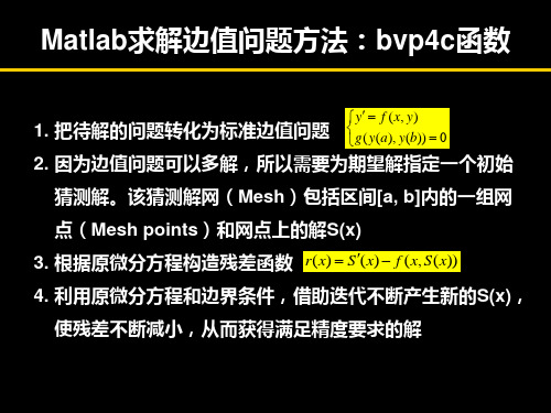
y1 y , y2 y1
原方程组等价于以下标准形式的 方程组:
y y 1 2 y2 (1 x 2 ) y1 1
边界条件为:
y1 (0) 1 0 y1 (1) 3 0
边值问题的求解
求解:
c=1; solinit=bvpinit(linspace(0,4,10),[1 1]); sol=bvp4c(@ODEfun,@BCfun,solinit,[],c); x=[0:0.1:4]; y=deval(sol,x); plot(x,y(1,:),'b-',sol.x,sol.y(1,:),'ro') legend('解曲线','初始网格点解') % 定义ODEfun函数 function dydx=ODEfun(x,y,c) dydx=[y(2);-c*abs(y(1))]; % 定义BCfun函数 function bc=BCfun(ya,yb,c) bc=[ya(1);yb(1)+2];
z(0) 1, z (0) 0, z ( ) 0
本例中,微分方程与参数λ的数值有关。一般而言,对于任意的λ值,该问题无解, 但对于特殊的λ值(特征值),它存在一个解,这也称为微分方程的特征值问题。 对于此问题,可在bvpinit中提供参数的猜测值,然后重复求解BVP得到所需的 参数,返回参数为sol.parameters
边值问题的求解
如果取1,计算结果如何?
infinity=6; solinit=bvpinit(linspace(0,infinity,5),[0 0 1]); options=bvpset('stats','on'); sol=bvp4c(@ODEfun,@BCfun,solinit,options); eta=sol.x; f=sol.y; fprintf('\n'); 2 求解: f ff (1 ( f ) ) 0 fprintf('Cebeci & Keller report f''''(0)=0.92768.\n') fprintf('Value computed here is f''''(0)=%7.5f.\n',f(3,1)) 0.5 clf reset plot(eta,f(2,:)); axis([0 infinity 0 1.4]); title... f (0) 0, f (0) 0, ('Falkner-Skan equation, positive wall shear,\beta=0.5.') 边界条件: f ( ) 1, xlabel('\eta'),ylabel('df/d\eta'),shg % 定义ODEfun函数 function dfdeta=ODEfun(eta,f) beta=0.5; dfdeta=[f(2);f(3);-f(1)*f(3)-beta*(1-f(2)^2)]; % 定义BCfun函数 function res=BCfun(f0,finf) res=[f0(1);f0(2);finf(2)-1];
随机森林GLS包使用指南说明书
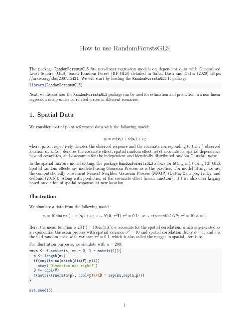
How to use RandomForestsGLSThe package RandomForestsGLSfits non-linear regression models on dependent data with Generalised Least Square(GLS)based Random Forest(RF-GLS)detailed in Saha,Basu and Datta(2020)https: ///abs/2007.15421.We will start by loading the RandomForestsGLS R package.library(RandomForestsGLS)Next,we discuss how the RandomForestsGLS package can be used for estimation and prediction in a non-linear regression setup under correlated errors in different scenarios.1.Spatial DataWe consider spatial point referenced data with the following model:y i=m(x i)+w(s i)+ i;where,y i,x i respectively denotes the observed response and the covariate corresponding to the i th observed location s i.m(x i)denotes the covariate effect,spatial random effect,w(s)accounts for spatial dependence beyond covariates,and accounts for the independent and identically distributed random Gaussian noise. In the spatial mixture model setting,the package RandomForestsGLS allows forfitting m(.)using RF-GLS. Spatial random effects are modeled using Gaussian Process as is the practice.For modelfitting,we use the computationally convenient Nearest Neighbor Gaussian Process(NNGP)(Datta,Banerjee,Finley,and Gelfand(2016)).Along with prediction of the covariate effect(mean function)m(.)we also offer kriging based prediction of spatial responses at new location.IllustrationWe simulate a data from the following model:y i=10sin(πx i)+w(s i)+ i; ∼N(0,τ2I),τ2=0.1;w∼exponential GP;σ2=10;φ=1. Here,the mean function is E(Y)=10sin(πX);w accounts for the spatial correlation,which is generated as a exponential Gaussian process with spatial varianceσ2=10and spatial correlation decayφ=1;and is the i.i.d random noise with varianceτ2=0.1,which is also called the nugget in spatial literature.For illustration purposes,we simulate with n=200:rmvn<-function(n,mu=0,V=matrix(1)){p<-length(mu)if(any(is.na(match(dim(V),p))))stop("Dimension not right!")D<-chol(V)t(matrix(rnorm(n*p),ncol=p)%*%D+rep(mu,rep(n,p)))}set.seed(5)n<-200coords<-cbind(runif(n,0,1),runif(n,0,1))set.seed(2)x<-as.matrix(runif(n),n,1)sigma.sq=10phi=1tau.sq=0.1D<-as.matrix(dist(coords))R<-exp(-phi*D)w<-rmvn(1,rep(0,n),sigma.sq*R)y<-rnorm(n,10*sin(pi*x)+w,sqrt(tau.sq))ModelfittingIn the package RandomForestsGLS,the working precision matrix used in the GLS-loss are NNGP approxima-tions of precision matrices corresponding to Matérn covariance function.In order tofit the model,the code requires:•Coordinates(coords):an n×2matrix of2-dimensional locations.•Response(y):an n length vector of response at the observed coordinates.•Covariates(X):an n×p matrix of the covariates in the observation coordinates.•Covariates for estimation(Xtest):an ntest×p matrix of the covariates where we want to estimate the function.Must have identical variables as that of X.Default is X.•Minimum size of leaf nodes(nthsize):We recommend not setting this value too small,as that will lead to very deep trees that takes a lot of time to be built and can produce unstable estimates.Default value is20.•The parameters corresponding to the covariance function(detailed afterwards).For the details on choice of other parameters,please refer to the helpfile of the code RFGLS_estimate_spatial, which can be accessed with?RFGLS_estimate_spatial.Known Covariance ParametersIf the covariance parameters are known,we set param_estimate=FALSE(default value);the code additionally requires the following:•Covariance Model(cov.model):Supported keywords are:“exponential”,“matern”,“spherical”,and “gaussian”for exponential,Matérn,spherical and Gaussian covariance function respectively.Default value is“exponential”.•σ2(sigma.sq):The spatial variance.Default value is1.•τ2(tau.sq):The nugget.Default value is0.01.•φ(phi):The spatial correlation decay parameter.Default value is5.•ν(nu):The smoothing parameter corresponding to the Matérn covariance function.Default value is0.5.We canfit the model as follows:set.seed(1)est_known<-RFGLS_estimate_spatial(coords,y,x,ntree=50,cov.model="exponential",nthsize=20,sigma.sq=sigma.sq,tau.sq=tau.sq,phi=phi)The estimate of the function at the covariates Xtest is given in estimation_reult$predicted.For inter-pretation of the rest of the outputs,please see the helpfile of the code RFGLS_estimate_ing covariance models other than exponential model are in beta testing stage.Unknown Covariance ParametersIf the covariance parameters are not known we set param_estimate=TRUE;the code additionally requires the covariance model(cov.model)to be used for parameter estimation prior to RF-GLSfitting.Wefit the model with unknown covariance parameters as follows.set.seed(1)est_unknown<-RFGLS_estimate_spatial(coords,y,x,ntree=50,cov.model="exponential",nthsize=20,param_estimate=TRUE)Prediction of mean functionGiven afitted model using RFGLS_estimate_spatial,we can estimate the mean function at new covariate values as follows:Xtest<-matrix(seq(0,1,by=1/10000),10001,1)RFGLS_predict_known<-RFGLS_predict(est_known,Xtest)Performance comparisonWe obtain the Mean Integrated Squared Error(MISE)of the estimateˆm from RF-GLS on[0,1]and compare it with that corresponding to the classical Random Forest(RF)obtained using package randomForest(with similar minimum nodesize,nodesize=20,as default nodesize performs worse).We see that our method has a significantly smaller MISE.Additionally,we show that the MISE obtained with unknown parameters in RF-GLS is comparable to that of the MISE obtained with known covariance parameters.library(randomForest)set.seed(1)RF_est<-randomForest(x,y,nodesize=20)RF_predict<-predict(RF_est,Xtest)#RF MISEmean((RF_predict-10*sin(pi*Xtest))^2)#>[1]8.36778#RF-GLS MISEmean((RFGLS_predict_known$predicted-10*sin(pi*Xtest))^2)#>[1]0.150152RFGLS_predict_unknown<-RFGLS_predict(est_unknown,Xtest)#RF-GLS unknown MISEmean((RFGLS_predict_unknown$predicted-10*sin(pi*Xtest))^2)#>[1]0.1851928We plot the true m(x)=10sin(πx)along with the loess-smoothed version of estimatedˆm(.)obtained from RF-GLS and RF where we show that RF-GLS estimate approximates m(x)better than that corresponding to RF.rfgls_loess_10<-loess(RFGLS_predict_known$predicted~c(1:length(Xtest)),span=0.1)rfgls_smoothed10<-predict(rfgls_loess_10)rf_loess_10<-loess(RF_predict~c(1:length(RF_predict)),span=0.1)rf_smoothed10<-predict(rf_loess_10)xval<-c(10*sin(pi*Xtest),rf_smoothed10,rfgls_smoothed10)xval_tag<-c(rep("Truth",length(10*sin(pi*Xtest))),rep("RF",length(rf_smoothed10)), rep("RF-GLS",length(rfgls_smoothed10)))plot_data<-as.data.frame(xval)plot_data$Methods<-xval_tagcoval<-c(rep(seq(0,1,by=1/10000),3))plot_data$Covariate<-covallibrary(ggplot2)ggplot(plot_data,aes(x=Covariate,y=xval,color=Methods))+geom_point()+labs(x="x")+labs(y="f(x)")Prediction of spatial responseGiven afitted model using RFGLS_estimate_spatial,we can predict the spatial response/outcome at new locations provided the covariates at that location.This approach performs kriging at a new location using the mean function estimates at the corresponding covariate values.Here we partition the simulated data into training and test sets in4:1ratio.Next we perform prediction on the test set using a modelfitted on the training set.est_known_short<-RFGLS_estimate_spatial(coords[1:160,],y[1:160],matrix(x[1:160,],160,1),ntree=50,cov.model="exponential",nthsize=20,param_estimate=TRUE)RFGLS_predict_spatial<-RFGLS_predict_spatial(est_known_short,coords[161:200,],matrix(x[161:200,],40,1))pred_mat<-as.data.frame(cbind(RFGLS_predict_spatial$prediction,y[161:200]))colnames(pred_mat)<-c("Predicted","Observed")ggplot(pred_mat,aes(x=Observed,y=Predicted))+geom_point()+geom_abline(intercept=0,slope=1,color="blue")+ylim(0,16)+xlim(0,16)Misspecification in covariance modelThe following example considers a setting when the parameters are estimated from a misspecified covariance model.We simulate the spatial correlation from a Matérn covariance function with smoothing parameter ν=1.5.Whilefitting the RF-GLS,we estimate the covariance parameters using an exponential covariance model(ν=0.5)and show that the obtained MISE can compare favorably to that of classical RF.#Data simulation from matern with nu=1.5nu=3/2R1<-(D*phi)^nu/(2^(nu-1)*gamma(nu))*besselK(x=D*phi,nu=nu)diag(R1)<-1set.seed(2)w<-rmvn(1,rep(0,n),sigma.sq*R1)y<-rnorm(n,10*sin(pi*x)+w,sqrt(tau.sq))#RF-GLS with exponential covarianceset.seed(3)est_misspec<-RFGLS_estimate_spatial(coords,y,x,ntree=50,cov.model="exponential",nthsize=20,param_estimate=TRUE)RFGLS_predict_misspec<-RFGLS_predict(est_misspec,Xtest)#RFset.seed(4)RF_est<-randomForest(x,y,nodesize=20)RF_predict<-predict(RF_est,Xtest)#RF-GLS MISEmean((RFGLS_predict_misspec$predicted-10*sin(pi*Xtest))^2)#>[1]0.1380569#RF MISEmean((RF_predict-10*sin(pi*Xtest))^2)#>[1]2.2956392.Autoregressive Time Series DataRF-GLS can also be used for function estimation in a time series setting under autoregressive errors.We consider time series data with errors from an AR(q)process as follows:y t=m(x t)+e t;e t=qi=1ρi e t−i+ηtwhere,y i,x i denotes the response and the covariate corresponding to the t th time point,e t is an AR(q) pprocess,ηt denotes the i.i.d.white noise and(ρ1,···,ρq)are the model parameters that captures the dependence of e t on(e t−1,···,e t−q).In the AR time series scenario,the package RandomForestsGLS allows forfitting m(.)using RF-GLS.RF-GLS exploits the sparsity of the closed form precision matrix of the AR process for modelfitting and prediction of mean function m(.).IllustrationHere,we simulate from the AR(1)process as follows:y=10sin(πx)+e;e t=ρe t−1+ηt;ηt∼N(0,σ2);e1=η1;ρ=0.9;σ2=10.Here,E(Y)=10sin(πX);e which is an AR(1)process,accounts for the temporal correlation,σ2denotes the variance of white noise part of the AR(1)process andρcaptures the degree of dependence of e t on e t−1. For illustration purposes,we simulate with n=200:rho<-0.9set.seed(1)b<-rhos<-sqrt(sigma.sq)eps=arima.sim(list(order=c(1,0,0),ar=b),n=n,rand.gen=rnorm,sd=s)y<-c(eps+10*sin(pi*x))ModelfittingIn case of time series data,the code requires:•Response(y):an n length vector of response at the observed time points.•Covariates(X):an n×p matrix of the covariates in the observation time points.•Covariates for estimation(Xtest):an ntest×p matrix of the covariates where we want to estimate the function.Must have identical variables as that of X.Default is X.•Minimum size of leaf nodes(nthsize):We recommend not setting this value too small,as that will lead to very deep trees that takes a lot of time to be built and can produce unstable estimates.Default value is20.•The parameters corresponding to the AR process(detailed afterwards).For the details on choice of other parameters,please refer to the helpfile of the code RFGLS_estimate_timeseries, which can be accessed with?RFGLS_estimate_timeseries.Known AR process ParametersIf the AR process parameters are known we set param_estimate=FALSE(default value);the code additionally requires lag_params=c(ρ1,···,ρq).We canfit the model as follows:set.seed(1)est_temp_known<-RFGLS_estimate_timeseries(y,x,ntree=50,lag_params=rho,nthsize=20) Unknown AR process ParametersIf the AR process parameters are not known,we set param_estimate=TRUE;the code requires the orderof the AR process,which is obtained from the length of the lag_params input vector.Hence if we want to estimate the parameters from a AR(q)process,lag_params should be any vector of length q.Here wefit the model with q=1set.seed(1)est_temp_unknown<-RFGLS_estimate_timeseries(y,x,ntree=50,lag_params=rho,nthsize=20,param_estimate=TRUE) Prediction of mean functionThis part of time series data analysis is identical to that corresponding to the spatial data.Xtest<-matrix(seq(0,1,by=1/10000),10001,1)RFGLS_predict_temp_known<-RFGLS_predict(est_temp_known,Xtest)Here also,similar to the spatial data scenario,RF-GLS outperforms classical RF in terms of MISE both with true and estimated AR process parameters.library(randomForest)set.seed(1)RF_est_temp<-randomForest(x,y,nodesize=20)RF_predict_temp<-predict(RF_est_temp,Xtest)#RF MISEmean((RF_predict_temp-10*sin(pi*Xtest))^2)#>[1]7.912517#RF-GLS MISEmean((RFGLS_predict_temp_known$predicted-10*sin(pi*Xtest))^2)#>[1]2.471876RFGLS_predict_temp_unknown<-RFGLS_predict(est_temp_unknown,Xtest)#RF-GLS unknown MISEmean((RFGLS_predict_temp_unknown$predicted-10*sin(pi*Xtest))^2)#>[1]0.8791857Misspecification in AR process orderWe consider a scenario where the order of autoregression used for RF-GLS modelfitting is mis-specified.We simulate the AR errors from an AR(2)process andfit RF-GLS with an AR(1)process.#Simulation from AR(2)processrho1<-0.7rho2<-0.2set.seed(2)b<-c(rho1,rho2)s<-sqrt(sigma.sq)eps=arima.sim(list(order=c(2,0,0),ar=b),n=n,rand.gen=rnorm,sd=s)y<-c(eps+10*sin(pi*x))#RF-GLS with AR(1)set.seed(3)est_misspec_temp<-RFGLS_estimate_timeseries(y,x,ntree=50,lag_params=0,nthsize=20,param_estimate=TRUE)RFGLS_predict_misspec_temp<-RFGLS_predict(est_misspec_temp,Xtest)#RFset.seed(4)RF_est_temp<-randomForest(x,y,nodesize=20)RF_predict_temp<-predict(RF_est_temp,Xtest)#RF-GLS MISEmean((RFGLS_predict_misspec_temp$predicted-10*sin(pi*Xtest))^2)#>[1]1.723218#RF MISEmean((RF_predict_temp-10*sin(pi*Xtest))^2)#>[1]3.735003ParallelizationFor RFGLS_estimate_spatial,RFGLS_estimate_timeseries,RFGLS_predict and RFGLS_predict_spatial one can also take the advantage of parallelization,contingent upon the availability of multiple cores.The component h in all the functions determines the number of cores to be used.Here we demonstrate an example with h=2.#simulation from exponential distributionset.seed(5)n<-200coords<-cbind(runif(n,0,1),runif(n,0,1))set.seed(2)x<-as.matrix(runif(n),n,1)sigma.sq=10phi=1tau.sq=0.1nu=0.5D<-as.matrix(dist(coords))R<-exp(-phi*D)w<-rmvn(1,rep(0,n),sigma.sq*R)y<-rnorm(n,10*sin(pi*x)+w,sqrt(tau.sq))#RF-GLS model fitting and prediction with parallel computationset.seed(1)est_known_pl<-RFGLS_estimate_spatial(coords,y,x,ntree=50,cov.model="exponential",nthsize=20,sigma.sq=sigma.sq,tau.sq=tau.sq,phi=phi,h=2)RFGLS_predict_known_pl<-RFGLS_predict(est_known_pl,Xtest,h=2)#MISE from single coremean((RFGLS_predict_known$predicted-10*sin(pi*Xtest))^2)#>[1]0.150152#MISE from parallel computationmean((RFGLS_predict_known_pl$predicted-10*sin(pi*Xtest))^2)#>[1]0.150152For RFGLS_estimate_spatial with very small dataset(n)and small number of trees(ntree),communi-cation overhead between the nodes for parallelization outweighs the benefits of the parallel computing hence it is recommended to parallelize only for moderately large n and/or ntree.It is strongly recommended that the max value of h is kept strictly less than the number of total cores available. Parallelization for RFGLS_estimate_timeseries can be addressed identically.For RFGLS_predict and RFGLS_predict_spatial,even for large dataset,single core performance is very fast,hence unless ntest and ntree are very high,we do not recommend using parallelization for RFGLS_predict and RFGLS_predict_spatial.。
glsl内联函数
glsl内联函数GLSL(OpenGL着色语言)是一种用于编写OpenGL程序的编程语言。
在GLSL中,内联函数是一种特殊的函数,可以直接在着色器代码中定义和使用。
本文将介绍GLSL内联函数的概念、定义与使用,以及其在实际编程中的应用实例。
1.GLSL内联函数概述GLSL内联函数是一种特殊的函数,与普通函数相比,它在编译时会被直接替换为函数体,而不是作为一个独立的函数调用。
这使得内联函数具有更高的执行效率,因为避免了函数调用的开销。
同时,内联函数也可以实现一些简单的功能,例如数学运算、类型转换等。
2.GLSL内联函数的定义与使用在GLSL中,内联函数的定义与普通函数相似,但需要使用`inline`关键字声明。
例如,以下是一个简单的内联函数,用于计算两个向量的和:```glslinline vec2 add(vec2 a, vec2 b) {return a + b;}```使用内联函数时,只需在需要调用函数的地方直接写上函数名,并传入所需的参数。
例如,要使用上述内联函数计算两个向量的和,可以这样写:```glslvec2 sum = add(vec2(1, 2), vec2(3, 4));```3.GLSL内联函数的优缺点优点:- 内联函数具有较高的执行效率,因为避免了函数调用的开销。
- 内联函数可以实现一些简单的功能,方便开发者进行编程。
缺点:- 内联函数可能导致代码可读性降低,尤其是当函数体较长时。
- 内联函数过多可能会导致着色器代码体积膨胀,增加编译时间。
4.内联函数在GLSL编程中的应用实例以下是一个使用内联函数实现在顶点着色器中计算两点之间距离的例子:```glslinline float distance(vec2 a, vec2 b) {return sqrt(pow(a.x - b.x, 2) + pow(a.y - b.y, 2));}void main() {vec2 posA = vec2(10, 20);vec2 posB = vec2(30, 40);float dist = distance(posA, posB);// 后续代码}```5.总结GLSL内联函数是一种在编译时直接替换为函数体的特殊函数,具有较高的执行效率。
GLSL语法入门

GLSL语法⼊门变量GLSL的变量命名⽅式与C语⾔类似。
变量的名称可以使⽤字母,数字以及下划线,但变量名不能以数字开头,还有变量名不能以gl_作为前缀,这个是GLSL保留的前缀,⽤于GLSL的内部变量。
当然还有⼀些GLSL保留的名称是不能够作为变量的名称的。
基本类型除了布尔型,整型,浮点型基本类型外,GLSL还引⼊了⼀些在着⾊器中经常⽤到的类型作为基本类型。
这些基本类型都可以作为结构体内部的类型。
如下表:类型描述void跟C语⾔的void类似,表⽰空类型。
作为函数的返回类型,表⽰这个函数不返回值。
bool布尔类型,可以是true 和false,以及可以产⽣布尔型的表达式。
int整型代表⾄少包含16位的有符号的整数。
可以是⼗进制的,⼗六进制的,⼋进制的。
float浮点型bvec2包含2个布尔成分的向量bvec3包含3个布尔成分的向量bvec4包含4个布尔成分的向量ivec2包含2个整型成分的向量ivec3包含3个整型成分的向量ivec4包含4个整型成分的向量mat2 或者 mat2x22×2的浮点数矩阵类型mat3或者mat3x33×3的浮点数矩阵类型mat4x44×4的浮点矩阵mat2x32列3⾏的浮点矩阵(OpenGL的矩阵是列主顺序的)mat2x42列4⾏的浮点矩阵mat3x23列2⾏的浮点矩阵mat3x43列4⾏的浮点矩阵mat4x24列2⾏的浮点矩阵mat4x34列3⾏的浮点矩阵sampler1D⽤于内建的纹理函数中引⽤指定的1D纹理的句柄。
只可以作为⼀致变量或者函数参数使⽤sampler2D⼆维纹理句柄sampler3D三维纹理句柄samplerCube cube map纹理句柄sampler1DShadow⼀维深度纹理句柄sampler2DShadow⼆维深度纹理句柄结构体结构体结构体可以组合基本类型和数组来形成⽤户⾃定义的类型。
在定义⼀个结构体的同时,你可以定义⼀个结构体实例。
Principles of Biochemistry 习题答案chapter 6

moles of each enzyme in cell volume of cell in liters 1.6 mm3
pr2h (3.14)(0.50 mm)2(2.0 mm) 1.6 10 12 cm3 1.6 10 12 mL 1.6 10 15 L Amount (in moles) of each enzyme in cell is (0.20)(1.2 g/cm3)(1.6 mm3)(10 12 cm3/mm3) (100,000 g/mol)(1000) 3.8 10
21
mol
Average molar concentration
3.8 10 21 mol 1.6 10 15 L 2.4 10
6
mol/L
2.4
10
6
M
S-63
2608T_ch06sm_S63-S77
2/1/08
7:34AM
Page S-64 ntt 102:WHQY028:Solutions Manual:Ch-06:
2608T_ch06sm_S63-S77
2/1/08
7:34AM
Page S-63 ntt 102:WHQY028:Solutions Manual:Ch-06:chpterEnzymes
6
1. Keeping the Sweet Taste of Corn The sweet taste of freshly picked corn (maize) is due to the high level of sugar in the kernels. Store-bought corn (several days after picking) is not as sweet, because about 50% of the free sugar is converted to starch within one day of picking. To preserve the sweetness of fresh corn, the husked ears can be immersed in boiling water for a few minutes (“blanched”) then cooled in cold water. Corn processed in this way and stored in a freezer maintains its sweetness. What is the biochemical basis for this procedure? Answer After an ear of corn has been removed from the plant, the enzyme-catalyzed conversion of sugar to starch continues. Inactivation of these enzymes slows down the conversion to an imperceptible rate. One of the simplest techniques for inactivating enzymes is heat denaturation. Freezing the corn lowers any remaining enzyme activity to an insignificant level. 2. Intracellular Concentration of Enzymes To approximate the actual concentration of enzymes in a bacterial cell, assume that the cell contains equal concentrations of 1,000 different enzymes in solution in the cytosol and that each protein has a molecular weight of 100,000. Assume also that the bacterial cell is a cylinder (diameter 1.0 mm, height 2.0 mm), that the cytosol (specific gravity 1.20) is 20% soluble protein by weight, and that the soluble protein consists entirely of enzymes. Calculate the average molar concentration of each enzyme in this hypothetical cell. Answer There are three different ways to approach this problem. (i) The concentration of total protein in the cytosol is (1.2 g/mL)(0.20) 100,000 g/mol 0.24 10
gls和稳健标准误处理方法

gls和稳健标准误处理方法GLS(Generalized Least Squares)和稳健标准误处理方法都是在统计学中用于处理回归分析中可能存在的问题的方法。
首先,让我们来看GLS。
GLS是一种回归分析方法,它可以处理误差项的异方差性(heteroscedasticity)。
在普通最小二乘法(OLS)中,我们通常假设误差项的方差是恒定的,但在现实数据中,误差项的方差可能并不是恒定的,而是随着自变量的变化而变化。
GLS通过对误差项进行加权,可以有效地处理异方差性,使得回归系数的估计更加准确。
而稳健标准误处理方法则是用于处理回归分析中可能存在的异方差性和异方差性之外的其他问题,比如数据中可能存在的异方差性、自相关性(autocorrelation)和异方差性。
稳健标准误可以有效地处理这些问题,使得回归系数的估计更加准确和可靠。
从另一个角度来看,GLS和稳健标准误处理方法都是在回归分析中用于提高估计的准确性和可靠性的方法。
通过使用这些方法,我们可以更好地理解自变量与因变量之间的关系,从而做出更加准确的预测和推断。
此外,这些方法也需要在实际应用中谨慎选择,因为不正确的方法选择可能会导致错误的推断和结论。
因此,在使用GLS和稳健标准误处理方法时,需要对数据和模型进行充分的检验和分析,以确保选择的方法是合适的,并且能够有效地处理数据中可能存在的问题。
总而言之,GLS和稳健标准误处理方法都是在统计学中用于处理回归分析中可能存在的问题的方法,它们可以帮助我们更准确地估计回归系数,并做出可靠的推断和预测。
在使用这些方法时,需要谨慎选择,并对数据和模型进行充分的检验和分析。
GLS简易操作手册
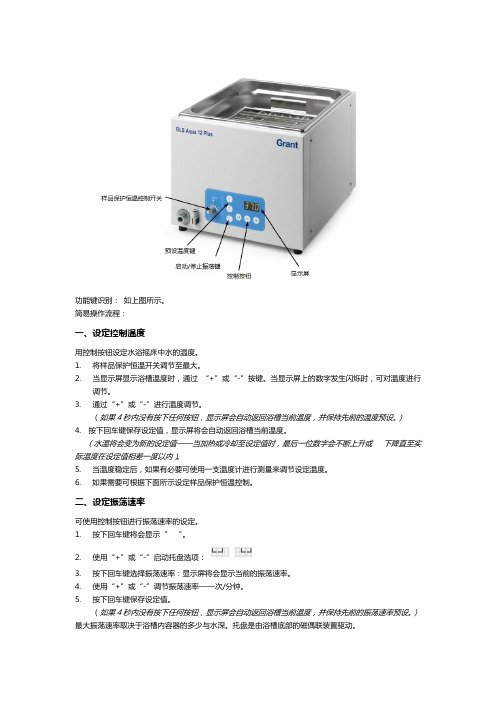
功能键识别:如上图所示。
简易操作流程:一、设定控制温度用控制按钮设定水浴摇床中水的温度。
1.将样品保护恒温开关调节至最大。
2.当显示屏显示浴槽温度时,通过“+”或“-”按键。
当显示屏上的数字发生闪烁时,可对温度进行调节。
3.通过“+”或“-”进行温度调节。
(如果4秒内没有按下任何按钮,显示屏会自动返回浴槽当前温度,并保持先前的温度预设。
)4. 按下回车键保存设定值,显示屏将会自动返回浴槽当前温度。
(水温将会变为新的设定值——当加热或冷却至设定值时,最后一位数字会不断上升或下降直至实际温度在设定值相差一度以内)。
5. 当温度稳定后,如果有必要可使用一支温度计进行测量来调节设定温度。
6. 如果需要可根据下面所示设定样品保护恒温控制。
二、设定振荡速率可使用控制按钮进行振荡速率的设定。
1.按下回车键将会显示“”。
2.使用“+”或“-”启动托盘选项:3.按下回车键选择振荡速率:显示屏将会显示当前的振荡速率。
4.使用“+”或“-”调节振荡速率——次/分钟。
5.按下回车键保存设定值。
(如果4秒内没有按下任何按钮,显示屏会自动返回浴槽当前温度,并保持先前的振荡速率预设。
)最大振荡速率取决于浴槽内容器的多少与水深。
托盘是由浴槽底部的磁偶联装置驱动。
三、启动&停止振荡用户可在任何时间通过“”启动或停止振荡。
停止键按下,托盘立即停止运动,但是启动振荡时,托盘将会缓慢加速至预设速率。
当使用“"启动振荡时,显示屏上将会短暂的显示当前的振荡速率。
四、设定样品保护恒温开关摇床配备有样品保护恒温开关用于保护样品。
该装置不是安全保护装置。
样品保护恒温开关只是用于将温度设置高于浴槽设定温度。
1.将样品保护恒温开关调节至最大。
2.将浴槽控制温度设置高于预定工作温度2℃并等待温度稳定。
3.逆时针旋转样品保护恒温开关直至听到”滴答“声。
摇床将会持续发出声音警报提示当前浴槽由样品保护恒温装置控制。
4. 使用”+‘或“-”重新调节至预定工作温度。
gls函数
GLS函数中的特定函数1. 函数定义GLS(Generalized Least Squares)函数是一种广义最小二乘法,用于估计线性回归模型中的参数。
GLS函数可以处理数据中存在异方差(heteroscedasticity)和自相关(autocorrelation)的情况,这使得它在许多实际问题中具有广泛的应用。
2. 函数用途GLS函数用于解决普通最小二乘法(OLS)无法有效处理的数据分析问题。
在许多实际情况下,数据可能不满足OLS假设,即误差项具有相同的方差和无相关性。
这种情况下,使用GLS函数可以提供更准确和有效的参数估计。
具体而言,GLS函数主要用于以下两种情况:2.1 异方差处理异方差指误差项的方差不是恒定的,在不同的条件下可能会发生变化。
这种情况下,使用OLS方法进行参数估计就会导致结果不准确。
GLS函数通过对误差项进行加权来解决异方差问题,使得对参数估计更加准确。
2.2 自相关处理自相关指误差项之间存在相关性,即一个误差项可能受到前面误差项的影响。
在存在自相关的数据中,使用OLS方法估计的参数也会失真。
GLS函数通过引入协方差矩阵的逆来解决自相关问题,使得参数估计更加准确。
3. 函数工作方式GLS函数的工作方式可以分为以下几个步骤:3.1 构建模型首先,需要构建一个线性回归模型,其中包括自变量和因变量。
假设我们有一个包含n个样本观测值的数据集,可以表示为:Y = Xβ + ε其中,Y是n×1的因变量向量,X是n×k的自变量矩阵,β是k×1的参数向量,ε是n×1的误差项向量。
3.2 计算协方差矩阵接下来,需要对误差项进行加权处理。
首先,计算误差项ε的协方差矩阵Σ。
如果数据存在异方差和/或自相关,则协方差矩阵Σ不是一个对角阵。
3.3 估计权重矩阵根据协方差矩阵Σ,可以估计出一个权重矩阵W。
权重矩阵W用于对误差项进行加权处理,在GLS中起到关键作用。
Acyba GLS模块安装与配置指南说明书

1.Installation1.1 Manual installation (via zip file)To manually install the module, you have to extract the zip file under app/code/Acyba/GLS directory.The module run with dependencies to others modules, that you need to install. You can find them in the composer.json file of the module. To install them, you have to use the following command : composer require vendor_name/module_name:X.X.XWarning : to install the dependencies, you have to use the above command with module names and version numbers as declared in the composer.json file of GLS module.Once the GLS module and its dependencies are installed, please run the followings Magento commands :php magento setup:upgradephp magento setup:di:compile2. Configuration2.1 Shipping methodsThe module created a new GLS shipping method in Stores > Configuration > Sales > Shipping Methods.To activate the GLS shipping method on the website, it’s necessary to switch the “Enable”parameter on and fill up the fields “GLS webservice login” and “GLS webservice password” whose values are provided by GLS.Warning : to use the official GLS module for Magento 2, you have to be a GLS customer. The use of the different GLS shipping methods is subject to the acceptance of GLS general terms and conditions. The activation of the GLS shipping methods of this module have to match with the prices lists signed with GLS. For more information, please get in touch with your GLS commercial contact.If you’re not a GLS customer, please connect to www.gls-group.eu to discover all the GLS services and contact GLS.The module is provided with a default configuration and all these parameters are editable in the menu Stores > Configuration > Sales > Shipping Methods > GLS, your transport partner :Title: Label of the GLS shipping method group displayed on the websiteEnable: By default disabled when installing the module. Switch on to see GLS shippingmethods on the websiteGLS webservice login: Provided by GLSGLS webservice password: Provided by GLSMaximum package weight : Maximum package weight that GLS can carryGLS Chez vous : Enable or disable the “at home” shipping methodThis service match the following GLS offers:- Business Parcel for your national shipments- Euro Business Parcel for your European shipments- Global Business Parcel for your international shipmentsGLS Chez Vous setup: Configuration field, please see more explanations and examplesbelowGLS Chez Vous order: Set the order of appearance of the “at home” shipping method amongGLS shipping methodsGLS Chez Vous +: Enable or disable the “at home” shipping methodThis service match the GLS offer : Flex Delivery ServiceGLS Chez Vous + setup: Configuration field, please see more explanations and examplesbelowGLS Chez Vous + order: Set the order of appearance of the “at home” shipping methodamong GLS shipping methodsGLS Point Relais: Enable or disable the relay shipping methodThis service match the GLS offer: Shop Delivery ServiceGoogle Maps API Key: API key to use the relay shipping method to locate the relays on aGoogle Maps (See: 5.1 Generation of the Google Maps API Key to learn how to generate this key)GLS Point Relais setup: Configuration field, please see more explanations and examplesbelowGLS Point Relais order: Set the order of appearance of the relay shipping method amongGLS shipping methodsOnly XL shop search: Enable the display of XL relays only (disabled by default)GLS Avant 13H: Enable or disable the express shipment before 1pmThis service match the GLS offer: Express Parcel GuaranteedGLS Avant 13H setup: Configuration field, please see more explanations and examplesbelowGLS Avant 13H order: Set the order of appearance of the express shipping method amongGLS shipping methodsTracking URL: Used to generate shipment tracking URLDebug: Allow to enable the module debugging function for the shipping costs calculation(Advanced function for developer)GLS module order: set the order of appearance of the GLS shipping methods group amongother shipping methodsThe configuration fields use a PHP format syntax used by the OWEBIA module for Magento 2, whose documentation is here.For example, here is the provided configuration for at home shipment:1. title : label displayed on the website for this shipping method2. enabled : activation conditions for this method. In this example, the method will be displayedonly if the destination country is France3. price : shipping fees for this method. In this example, if the cart total weight is less than or equalto 150, the fees will be 5, if the cart total weight is less than or equal to 160, the fees will be 3 and in other cases, it will be 0It’s possible to add filters on customer group, product categories etc … (for more informations, please check documentation)Many methods can be created for one configuration field. To do that, you have to duplicate the addMethod function by defining others rules.Warning: in the method name (ex: tohome_fr above), only the part before the underscore can be edit2.2 GLS Advanced Setup2.2.1 General ConfigurationAgency code: GLS agency code you are linked to. Information provided by GLS2.2.2 Import/export configurationThis section contains the configuration to manage the import and export of GLS orders. For more information about import and export, please check 4. Import/Export.Active: Activation of automatic import/export through a cron taskFrequency: Cron task frequency in minutes (every X minutes)Cron expression: Cron expression generated from frequency field (if the you can't see themodification after saving, please refresh Magento configuration cache)Import folder: Folder in which there are the orders to importExport folder: Folder in which the exported orders are downloadedStatus of orders to export: Status of orders to export for automatic export through the crontask3. DisplayAfter the shipping methods configuration, here is an example of the display of these methods on the website:If the user choose the shipping method “Point Relais”, a popup to choose the relay to deliver to will be displayed:This way he can choose the relay by clicking the button “Choose this relay”.By clicking on markers on the map, the user can see relay opening hours:A confirmation popup will ask the user to confirm his choice:After confirmation, the relay details will be displayed below the shipping method:4. Import/Export4.1 Export to WinExpéThe module allows to export orders files to the GLS WinExpé software.The exports configuration is done in Stores > Configuration > Sales > GLS Advanced Setup (check 2.2.2 Import/export Configuration).This feature is reachable through a new menu entry “GLS IMPORT/EXPORT > Export orders”.In the configuration, the “Export Folder” parameter have to be well set.The export screen lists all orders whose shipping method is a GLS one. It’s possible to either download or export one or several orders. To do this, you have to check orders that you want to export, then choose in the “Actions” menu what you want to do.The “Download” option will download the generated file on your computer.The “Export” option will put the generated file in the directory set in configuration (Stores > Configuration > Sales > GLS Advanced Setup > Import / Export Configuration).You have to create a FTP access on this directory and configure it in WinExpé so the software can automatically recovers the files. For any question about the WinExpé software configuration, please get in touch with your GLS IT contact.4.2 Import from WinExpéThe module allows to import files from the GLS WinExpé software, to save tracking numbers in Magento.The imports configuration is done in Stores > Configuration > Sales > GLS Advanced Setup (check 2.2.2 Import/export Configuration).This feature is reachable through a new menu entry “GLS IMPORT/EXPORT > Import tracking numbers”.In the configuration, the “Import folder” parameter have to be well set.In the import screen you will find a button to import files that are in the folder set in the configuration (Stores > Configuration > Sales > GLS Advanced Setup > Import / Export Configuration). With these files, the tracking numbers will be added to the matching orders, then files will be deleted.You have to create a FTP access on this directory and configure it in WinExpé for the software can automatically upload the files to import.4.3 Automatic Import/ExportIt’s possible to automate orders import and export. It can be configured in Stores > Configuration > Sales > GLS Advanced Setup (check 2.2.2 Import/export Configuration).To enable this, you have to switch on the “Active” parameter in configuration (Stores > Configuration > Sales > GLS Advanced Setup > Import / Export Configuration > Active) and fill up the wanted frequency in minutes (Stores > Configuration > Sales > GLS Advanced Setup > Import / Export Configuration > Frequency).Then, Magento will export orders that have the defined status (Stores > Configuration > Sales > GLS Advanced Setup > Import / Export Configuration > Status of orders to export) and import orders at the defined frequency.5. Miscellaneous5.1 Generation of the Google Maps API KeyTo use the GLS Point Relais shipping method, it’s necessary to define an API key. Indeed, the module uses a Google Map to locate the relays, and this service require an API key.You have to generate this API Key and set it in the configuration (check 2.1 Shipping Methods). Here are the different steps to generate this API key:Go to https://Connect with a Google accountGo to “Credentials” sectionClick on “Create credentials” > “API Key” (It’s possible to configure restriction for this key)Copy the keyGo to “Library” sectionSearch “Google Maps JavaScript API” and click on the corresponding resultClick on “Enable”Back in the GLS configuration, paste the key in Stores > Configuration > Sales > ShippingMethods > GLS, your transport partner > Google Maps API Key5.2 SupportIf you need some help with the configuration or installation of our module, please contact yout GLS advisor。
wincc趋势控件y轴的数值效果

wincc趋势控件y轴的数值效果摘要:1.WinCC 趋势控件的概述2.WinCC 趋势控件的Y 轴数值效果3.Y 轴数值效果的应用实例4.Y 轴数值效果的优缺点分析5.总结正文:1.WinCC 趋势控件的概述WinCC 趋势控件是一款由西门子公司开发的用于监控和控制过程的软件工具。
它可以在计算机屏幕上显示实时的数据趋势,并可以对数据进行分析和处理。
WinCC 趋势控件具有强大的功能,可以满足各种工业自动化领域的需求。
2.WinCC 趋势控件的Y 轴数值效果WinCC 趋势控件的Y 轴数值效果是指在控件中,Y 轴所表示的数据值的变化情况。
这种效果可以通过设置不同的颜色、线条样式以及数据标签等方式来实现。
通过这些设置,用户可以更直观地了解数据的变化趋势,从而更好地进行数据分析和决策。
3.Y 轴数值效果的应用实例例如,在工业生产过程中,可以通过WinCC 趋势控件的Y 轴数值效果来实时监控生产数据的变化,如温度、压力、速度等。
这样,操作人员可以根据数据显示的变化趋势,及时调整生产参数,保证生产过程的稳定和安全。
4.Y 轴数值效果的优缺点分析优点:a) 通过直观的数据可视化,便于用户进行数据分析和决策。
b) 可以实时反映数据的变化趋势,有助于发现问题并及时处理。
c) 可以设置不同的颜色、线条样式以及数据标签,满足不同用户的需求。
缺点:a) 需要一定的计算机操作技能,对于操作不熟练的用户可能会有一定的难度。
b) 对于大量数据,可能会影响计算机的运行速度。
5.总结总的来说,WinCC 趋势控件的Y 轴数值效果是一个十分实用的功能,可以大大提高用户对于数据的理解和分析能力。
常见CVI编程错误

错误: int CVICALLBACK Loadfile (int panel, int control, int event,
void *callbackData, int eventData1, int eventData2) {
。。。。。。 。。。。。。
if (lStatus = VAL_EXISTING_FILE_SELECTED) {
错误原因:将函数 CVICALLBACK Acquire_display( )命名为 CVICALLBACK sin( ), 因 sin( )函数已被 C 语 言使用。
3. 实验二程序不能运行,错误提示:link errors
解决方法:在工程文件(.prj)中再添加三个文件:Imaq_CVI.h, Imaq_CVI.lib, Imaq_CVI.fp,这三个文件的 位置在:C:\CVI401\IMAQ_CVI\
CVI 编程常见错误
1. 实验一的第三个实验不能正确显示最大值、最小值(如图示) ........................................................... 2 2. 实验一不能显示正弦曲线 ........................................................................................................................... 2 3. 实验二程序不能运行,错误提示:link errors ..................................................................................... 2 4. 实验二不能显示图像 ................................................................................................................................... 2 5. CVI 不能显示图像 ........................................................................................................................................ 3 6. 实验二 中值滤波的 1 个问题 ..................................................................................................................... 3 7. 实验二不能显示面板 ................................................................................................................................... 3 8. 实验二不能进行均值滤波 ........................................................................................................................... 3 9. 实验二在均值滤波时,显示如下错误信息: ........................................................................................... 4 10. 实验三(直方图显示)中,不能显示直方图 ........................................................................................... 4 11. 实验指导书中实验三(边缘检测)的错误内容更正 ............................................................................... 4 12. 实验三的直方图均衡化实验时,程序不能运行,错误提示: ............................................................... 5 13. 实验五不能显示区域目标的数量,显示错误信息如下图所示: ........................................................... 6 14. 实验 5.3 的链接错误 .................................................................................................................................. 6 15. 实验 5.1 中形态学处理的 3 个问题: ....................................................................................................... 7 16. 形态学处理后的图像,原程序如下,显示结果是全黑(见下图),为什么? ..................................... 7 17. 关于彩色类函数 IPI_GetColorPixel 的使用问题: ................................................................................. 9 18. 如何批量调入图像(用于一键运行)? ................................................................................................... 9 19. 如果我要调用 ROI 中的 boundingRect,要怎样调用? .......................................................................... 10 20. 那些 if 语句,for 语句是不是要自己敲进去,有没有快捷的方法可以使用? ................................ 10 21. 在 user interface library 接口库找不到 GetCtrlIndex()函数,CVI 有没有函数查找功能? ... 10 22. 如何在图像中画一个方框? ..................................................................................................................... 11 24. 做实验二时遇到的问题:装入不了图像 ................................................................................................. 11 25. 实验一出现了问题:系统提示如下图所示: ......................................................................................... 12 26. 实验五.3 出现的问题——工程文件链接错误(project link errors) ......................................... 13 27. 实验五.3 出现的问题之二 ....................................................................................................................... 13 28. 程序打不开图像文件,显示错误信息#200 ............................................................................................. 14 29. 在图像的形态学处理实验(5.2)中,处理结果是漆黑一片,为什么? ........................................... 14 30. 语句 IPI_CloseSys();出现位置不对引起的#200 错误 ......................................................................... 15 31. 实验 5.1 中的细化处理结果不对,二值图像基本没有变化,但其他的形态学处理都会有变化,为什 么? 15 32. 利用函数 GetCtrlVal()时容易出现的几个错误 ................................................................................ 15 33. 我想利用函数 IPI_Histogram ()求整幅图像的灰度均值,请问我如何利用这个函数,得到的直方 图报告在哪里看到呢? ......................................................................................................................................... 16
glsl函数精度 -回复
glsl函数精度-回复GLSL函数精度GLSL(OpenGL Shading Language)是用于编写OpenGL程序中着色器的语言,包括顶点着色器和片段着色器。
在GLSL中使用的函数具有不同的精度,也就是计算结果的准确度。
本文将一步一步回答关于GLSL函数精度的问题。
1. 什么是函数精度?函数精度指的是函数计算结果的准确度或者是舍入误差。
在计算时,涉及到浮点数运算,因为浮点数无法精确地表示某些数字(例如无理数或非常大或非常小的数),所以计算结果会存在一定的误差。
这个误差可以体现为计算结果与真实结果之间的差异。
2. GLSL函数的精度有哪些?GLSL提供了几种不同的函数精度。
其中最常见的是highp、mediump和lowp。
这些精度限定符可以用于变量和函数参数上,在函数内部的计算也会受到精度的影响。
这些精度限定符定义了计算结果的最小有效位数,从而影响到计算的舍入误差。
3. 何时使用不同的函数精度?函数精度的选择应该根据计算的需求和性能的要求来决定。
一般来说,使用高精度(highp)可以获得更准确的计算结果,但也会消耗更多的计算资源。
如果计算结果不需要太高的精度,或者为了提高计算性能,可以使用中等精度(mediump)或低精度(lowp)。
4. 如何指定函数精度?要指定GLSL函数的精度,可以使用精度限定符。
例如,下面的代码演示了如何在GLSL中指定函数的精度:glslmediump float calculateDistance(vec3 pointA, vec3 pointB) { return length(pointA - pointB);}在上面的例子中,函数calculateDistance接受两个参数pointA和pointB,并返回它们之间的距离。
这个函数使用mediump精度来计算并返回浮点数。
5. 精度限定符的作用范围是什么?精度限定符的作用范围是函数本身以及函数内部的局部变量和参数。
glsl函数精度 -回复
glsl函数精度-回复GLSL(OpenGL着色语言)是一种专门为OpenGL而设计的着色器语言。
在编写GLSL着色器时,一个常见的问题是函数的精度。
函数精度是指函数计算结果的准确性和误差。
精度的选择对于图形渲染和计算来说非常重要,因为函数的结果可能会影响渲染的质量和效率。
在本文中,我们将探讨GLSL函数精度的相关问题。
首先,我们需要了解GLSL中函数的精度是如何定义和控制的。
GLSL提供了一些关键字来控制函数的精度,例如`highp`、`mediump`和`lowp`。
这些关键字会影响浮点数的计算精度,从而影响函数的结果。
`highp`表示高精度,`mediump`表示中等精度,`lowp`表示低精度。
在GLSL中,默认的函数精度是`highp`,这意味着函数的计算结果将以高精度表示。
与此同时,使用高精度的计算会消耗更多的资源,因此可能会导致性能下降。
为了提高性能,开发人员可以使用`mediump`或`lowp`来降低函数的计算精度。
当然,这也意味着可能会引入一些计算误差。
那么,我们如何选择函数的精度呢?选择函数的精度需要根据具体情况而定。
对于大多数图形渲染任务来说,`highp`已经足够满足需求,因为这些任务对于计算精度要求较高。
但是,对于一些计算密集型的任务,如物理模拟或计算机视觉算法,可以使用`mediump`或`lowp`来提高性能。
此外,还有一些情况需要特别注意。
例如,当两个函数精度不一致时,函数的计算结果可能会出现不可预测的误差。
这种情况下,可以使用函数精度转换操作符来统一精度,以避免这种问题。
函数精度转换操作符可以在不同精度的函数之间进行转换,以统一精度。
另一个需要注意的问题是函数的输入和输出精度。
函数的输入和输出精度也会影响函数的计算结果。
如果函数的输入是高精度的,而输出是低精度的,那么函数的计算结果可能会有较大的误差。
为了避免这种情况,可以在函数的参数列表中明确指定输入和输出的精度。
glscalef函数 -回复

glscalef函数-回复GLScalef函数是OpenGL中的一个函数,用于对当前矩阵进行缩放变换。
在这篇文章中,我们将逐步讨论GLScalef函数的作用、语法和使用方法,以及一些示例和注意事项。
首先,让我们来了解一下GLScalef函数的作用。
GLScalef函数可以用来对当前矩阵进行缩放变换,改变物体在三个坐标轴上的大小比例。
这对于实现缩放效果,使物体变大或变小,非常有用。
它可以在三维场景中实现一些特殊效果,如放大、缩小和形变。
GLScalef函数的语法如下:void glScalef(GLfloat x, GLfloat y, GLfloat z);GLScalef函数接受三个参数,分别表示在x、y和z轴上的缩放比例。
这些参数的取值可以是任意浮点数,它们通常是大于零的值。
当参数小于1时,物体会缩小;当参数大于1时,物体会放大。
如果参数为1,物体的大小不会改变。
使用GLScalef函数的一般步骤如下:1. 启用和设置投影矩阵或模型视图矩阵:在使用GLScalef函数之前,我们需要启用和设置之前定义的投影矩阵或模型视图矩阵。
这些矩阵用来定义场景的透视投影或物体的位置、旋转和大小。
2. 调用GLScalef函数:使用glScalef函数来对当前矩阵进行缩放变换。
传入的参数分别表示在x、y和z轴上的缩放比例。
3. 绘制物体:在进行缩放变换后,我们可以绘制物体。
这可以通过OpenGL中的其他绘图函数来实现,如glBegin和glEnd配合glVertex 等函数。
下面是一个使用GLScalef函数的示例代码片段:c++glMatrixMode(GL_MODELVIEW); 设置为模型视图矩阵模式glLoadIdentity(); 重置模型视图矩阵为单位矩阵glTranslatef(0.0f, 0.0f, -5.0f); 平移物体到适当的位置glRotatef(45.0f, 0.0f, 1.0f, 0.0f); 绕y轴旋转物体glScalef(2.0f, 2.0f, 2.0f); 放大物体两倍glBegin(GL_TRIANGLES);glVertex3f(0.0f, 1.0f, 0.0f);glVertex3f(-1.0f, -1.0f, 0.0f);glVertex3f(1.0f, -1.0f, 0.0f);glEnd();在上面的示例中,我们首先设置了模型视图矩阵,并对物体进行适当的平移和旋转。
glsl_es double三角函数 -回复
glsl_es double三角函数-回复GLSL_ES(OpenGL Shading Language for Embedded Systems)是一种用于嵌入式系统的OpenGL着色语言。
GLSL_ES是一种类似于C语言的编程语言,旨在为嵌入式设备提供高效的图形渲染和计算功能。
在GLSL_ES中,有许多内置函数可以进行各种数学和图形计算,其中包括三角函数。
在GLSL_ES中,有许多内置的三角函数可以被使用。
这些三角函数包括正弦函数(sin)、余弦函数(cos)、正切函数(tan)、反正弦函数(asin)、反余弦函数(acos)和反正切函数(atan)。
这些函数允许我们在图形渲染的过程中进行各种角度和距离的计算。
首先,让我们来看看正弦函数(sin)。
正弦函数接受一个角度作为参数,并返回对应的正弦值。
例如,sin(30)的返回值是0.5,表示30度对应的正弦值是0.5。
正弦函数在图形渲染中广泛应用,例如在计算光线的折射角、旋转和动画等方面。
接下来是余弦函数(cos),余弦函数与正弦函数非常相似,它也接受一个角度作为参数,并返回对应的余弦值。
例如,cos(60)的返回值是0.5,表示60度对应的余弦值是0.5。
余弦函数在图形渲染中同样非常常用,例如在计算光线的反射角、旋转和动画等方面。
正切函数(tan)是一个比较特殊的三角函数,它接受一个角度作为参数,并返回对应的正切值。
正切函数在图形渲染中也有一些应用,例如在计算物体之间的碰撞、阴影和投影等方面。
接下来是反正弦函数(asin),它接受一个值作为参数,并返回对应的角度。
例如,asin(0.5)的返回值是30度,表示正弦值为0.5的角度是30度。
反正弦函数在图形渲染中通常用于计算光线的折射角度、计算物体的旋转角度等方面。
反余弦函数(acos)与反正弦函数类似,它接受一个值作为参数,并返回对应的角度。
例如,acos(0.5)的返回值是60度,表示余弦值为0.5的角度是60度。
- 1、下载文档前请自行甄别文档内容的完整性,平台不提供额外的编辑、内容补充、找答案等附加服务。
- 2、"仅部分预览"的文档,不可在线预览部分如存在完整性等问题,可反馈申请退款(可完整预览的文档不适用该条件!)。
- 3、如文档侵犯您的权益,请联系客服反馈,我们会尽快为您处理(人工客服工作时间:9:00-18:30)。
文件夹加密:建立一个主文件夹(不要放在系统所在的分区C盘以确保系统出现问题时文件不丢失),例如D:\皇帝专用文件夹,在主文件夹里另建子文件夹如 “文件”、“图片”、“影片”、“其它”等子目录,而只需使用“秘密文件夹”加密主文件夹即可实现保护。这样的好处是在秘密文件夹里双击打开或解密一次该文件夹即可查阅使用所有的文件,非常方便用户的使用和解密恢复。
超级特工文Leabharlann /文件夹双重加密高强度加密保密强度高,加密后的文件有脱机保护防盗功能,脱离加密的电脑不能解密。文件夹加密超级特工软件采用了国际上最新的高安全性高强度的加密算法,国内首创双重加密模式确保用户的资料绝对安全。
双重加密的文件能不能拿到别的电脑上解密?
不能,双重加密的文件有脱机保护防盗功能,不能拿到别的电脑上解密!强制破解会破坏文件。
解密时出现该列表为空文件夹已解密或磁盘同级分区有重名文件夹.....的提示:
一是该文件夹已通过“救护”或“数据恢复”解密,只是列表中仍显示。
解决方法按提示移除即可
二是软件检测到磁盘同级目录下有同加密列表中相同名字的文件夹,为避免数据覆盖,操作将暂停。
解决方法:将磁盘同级目录下的文件夹改名后,再进行解密操作即可。
使用超级特工杀手锏时个别设置没有立即生效?
在超级特工杀手锏的近百项功能操作中,有些功能设置需要操作系统重新启动后才能生效,这些功能操作时都有相关的操作提示,按提示操作即可。
为什么要使用正版超级特工软件?
加密软件不同于其他软件,侧重于加密数据的高强度。网上的破解版或注册机会导致在一定情况下资料不完整或文件可能完全损坏丢失,所以请大家务必谨慎勿用,如果您确实需要加密自己或公司重要资料,买个正版是值得的,不要先尝试破解使用,否则到时候破解导致文件损失我们也无法帮助您。因此我们建议您宁愿使用试用版也不要所谓的盗版破解版,毕竟有些重要资料丢失的时候是无可挽回和估计的。
查看[如何正确的使用“救护”或“解密恢复”功能]
文件夹加密超级特工软件过期可以解密吗?
可以解密,软件过期“解密”功能正常使用,用户可以解密文件夹。文件夹加密超级特工过期后只是关闭“加密”和“高级”功能,如果需要继续使用“加密”和“高级”功能可以注册VIP永久使用详见[注册VIP]
老版本可以使用解密恢复功能恢复。(因盗用破解注册码导致软件出错不在此范围,不提供任何服务)
查看[文件夹加密超级特工怎样加密][使用秘笈]
文件夹加密超级特工秘密文件夹的文件夹加密是否支持最新操作系统Vista/Windows7文件夹加密?
全面支持Vista/Windows7文件夹加密,可以使用右键加密、智能检测自动恢复等所有功能
使用文件夹加密超级特工秘密文件夹进行文件/文件夹加密的保密强度高吗?
使用别人的注册码、系列号可以吗?
注册用户的注册码、系列号为注册用户所拥有,非《软件使用授权协议》条款许可使用他人的注册码、系列号是违法行为。使用他人的注册码、系列号盗版破解使用会导致数据库冲突、加密列表丢失和软件报错GLSCC关闭。出现此问题的用户可以注册正版后使用VIP版本的数据智能恢复或申请VIP技术支持恢复。参阅[申请VIP技术支持]
三是盘符变动,如移动磁盘、U盘盘符变化或重做系统导致的盘符变化。
解决方法:使用高级-救护功能-输入原来的盘符路径进行解密恢复操作即可。
文件夹加密文件夹加密超级特工秘密文件夹为何不允许加密系统文件夹?
系统运行时会调用相关系统文件、文件夹,如果加密系统文件、系统文件夹有可能会导致系统运行时不正常或崩溃。所以,不可以加密系统文件、系统文件夹。如果您不知道如何区分,最简单的方法就是操作系统安装后所有的自带文件夹都不要去进行文件夹加密操作,豪华版独创智能模块启用系统文件夹保护,新手也可以安全使用,任意加密而不必担心加密系统文件夹,智能保护安全无忧。
如何取消文件夹加密超级特工GLSCC-WJJ右键加密菜单?
启动GLSCC-WJJ,选择高级-系统功能-右键直接加密-取消。
如何取消超级特工桌面无形锁GLSSPY-ZM右键菜单和开机启动?
启动GLSSPY-ZM,选择特工无形锁-特工桌面无形锁系统设置-输入默认密码激活选项-不选择“开机启动特工桌面无形锁”和“右键ZMS桌面无形锁菜单”。GLSSPY-ZM默认密码为GLSSPY
文件/文件夹双重加密注意事项:
文件/文件夹双重加密或解密时请关闭杀毒软件或实时监控软件(测试NOD32无影响),避免干扰加密防止意外损坏文件(加密前请自行备份)。正在加密时不要在电脑上做其他的操作避免干扰影响,加密10MB的文件大约10秒时间,文件大小决定处理时间,应耐心等待完成,切勿强制关闭软件导致文件受损!过大的文件/文件夹加密时间长不建议使用双重加密。
只要在使用期内您重新安装一次同一版本文件夹加密超级特工秘密文件夹就可以使用软件功能打开加密文件夹。不同的版本可能会出现兼容问题,VIP版本智能数据恢复模式兼容所有版本。
如果我卸载了文件夹加密;超级特工秘密文件夹软件,加密文件夹会一起被卸载掉吗?
您可以放心,加密文件夹不会一起被卸载掉,因为软件的卸载与文件夹加密/解密无关。
正确的方法:bt下载完成100%后,点击停止,在没有上传、下载、播放的未使用状态下进行文件夹加密加密。
重装系统后文件夹加密超级特工秘密文件夹加密列表不显示?
重装操作系统,如果你格式化或GHOST覆盖的是系统C盘,则C盘以外加密的资料是不会丢失的,依旧安全的被加密中,当然您C盘加密的资料肯定不存在,所以以后加密的资料最好不要放在系统盘。免费用户可以使用文件夹加密超级特工软件的救护功能,输入原文件夹的完整路径进行救护操作解密恢复,VIP版本用户可以使用自动检测恢复功能恢复或联络VIP技术支持(申请VIP技术支持)。
非法盗版使用超级特工注册码数据出错怎么办?
请合法注册后联络VIP技术支持。[注册升级VIP]
客户支持软件相关问题
查看客户支持软件相关问题解答[点击这里] 更多文件夹加密超级特工秘密文件夹软件帮助查看[点击这里]
注册相关问题解答
查看注册相关问题解答[点击这里] 更多帮助信息查看[点击这里]
文件夹加密超级特工软件运行提示错误怎么办?
非法破解注册、非法盗用个人注册码/企业注册码、使用破解版等会都会导致软件出错无法运行,使用破解注册和盗用他人注册码均属于违法盗版行为,我们不提供任何技术支持!请合法注册后联络技术支持。
如果我卸载了文件夹加密超级特工秘密文件夹;这个软件,加密文件夹以后还能打开吗?
正确的方法:把要加密的数据放到自己新建的文件夹(建议不要放到C盘),再进行加密。
文件夹加密会占用更多的磁盘空间吗?
不会,因为文件夹加密文件夹加密超级特工秘密文件夹采用的是系统底层加密技术,它不会占用磁盘空间。
如何正确的对bt下载影片的文件夹进行文件夹加密?
很多用户都喜欢用文件夹加密超级特工闪电加密的功能来加密上百G大容量的影片目录,有些用户对bt正在下载的文件夹目录进行加密,但是这样加密会中断bt下载显示从零开始,而加密文件夹的影片也不完整。