数据、模型与决策(运筹学)课后习题和案例答案009s
《数据模型与决策》复习题及参考答案0

《数据模型与决策》复习题及参考答案一、填空题1.运筹学的主要研究对象是各种有组织系统的管理问题,经营活动。
2.运筹学的核心主要是运用数学方法研究各种系统的优化途径及方案,为决策者提供科学决策的依据。
3.模型是一件实际事物或现实情况的代表或抽象。
4通常对问题中变量值的限制称为约束条件,它可以表示成一个等式或不等式的集合。
5.运筹学研究和解决问题的基础是最优化技术,并强调系统整体优化功能。
运筹学研究和解决问题的效果具有连续性。
6.运筹学用系统的观点研究功能之间的关系。
7.运筹学研究和解决问题的优势是应用各学科交叉的方法,具有典型综合应用特性。
8.运筹学的发展趋势是进一步依赖于_计算机的应用和发展。
9.运筹学解决问题时首先要观察待决策问题所处的环境。
10.用运筹学分析与解决问题,是一个科学决策的过程。
11.运筹学的主要目的在于求得一个合理运用人力、物力和财力的最佳方案。
12.运筹学中所使用的模型是数学模型。
用运筹学解决问题的核心是建立数学模型,并对模型求解。
13用运筹学解决问题时,要分析,定议待决策的问题。
14.运筹学的系统特征之一是用系统的观点研究功能关系。
15.数学模型中,“s·t”表示约束。
16.建立数学模型时,需要回答的问题有性能的客观量度,可控制因素,不可控因素。
17.运筹学的主要研究对象是各种有组织系统的管理问题及经营活动。
二、单选题1.建立数学模型时,考虑可以由决策者控制的因素是( A )A.销售数量 B.销售价格 C.顾客的需求 D.竞争价格2.我们可以通过( C )来验证模型最优解。
A.观察 B.应用 C.实验 D.调查3.建立运筹学模型的过程不包括( A )阶段。
A.观察环境 B.数据分析 C.模型设计 D.模型实施4.建立模型的一个基本理由是去揭晓那些重要的或有关的( B )A数量 B变量 C 约束条件 D 目标函数5.模型中要求变量取值( D )A可正 B可负 C非正 D非负6.运筹学研究和解决问题的效果具有( A )A 连续性B 整体性C 阶段性D 再生性7.运筹学运用数学方法分析与解决问题,以达到系统的最优目标。
数据、模型与决策(运筹学)课后习题和案例答案008
CHAPTER 8 PERT/CPM MODELS FOR PROJECT MANAGEMENTReview Questions8.1-1 The bid is for $5.4 million with a penalty of $300,000 if the deadline of 47 weeks is notmet. In addition, a bonus of $150,000 will be paid if the plant is completed within 40 weeks.8.1-2 He has decided to focus on meeting the deadline of 47 weeks.8.1-3 An immediate predecessor is an activity that must be completed just prior to startingthe given activity. Given the immediate predecessors of an activity, this activity then becomes the immediate successor of each of these immediate predecessors.8.1-4 (1) the activities of the project; (2) the immediate predecessors of the activities; and (3)the estimated duration of the activities8.2-1 (1) activity information; (2) precedence relationships; and (3) time information(duration)8.2-2 In an AOA network, each activity is represented by an arc, while in an AON network,each activity is represented by a node. AON networks are being used here.8.2-3 The bars in a Gantt chart show the scheduled start and finish times for activities in aproject.8.3-1 (a) A path through a project network is one of the routes following the arrows (arcs)from the start node to the finish node; (b) the length of a path is the sum of the estimated durations of the activities on the path; (c) the longest path is called the critical path.8.3-2 (1) The actual duration of each activity must be the same as its estimated duration;and (2) each activity must begin as soon as all its immediate predecessors are finished.8.3-3 The earliest start time of an activity is equal to the largest of the earliest finish times ofits immediate predecessors.8.3-4 A forward pass is the process of starting with the initial activities and working forwardin time toward the final activities.8.3-5 It is a last chance schedule because anything later will delay the completion of theproject.8.3-6 The latest finish time of an activity is equal to the smallest of the latest start times ofits immediate successors.8.3-7 A backward pass starts with the final activities and works backward in time toward theinitial activities instead of starting with the initial activities.8.3-8 Any delay along the critical path will delay project completion.8.3-9 (1) Identify the longest path through the project network; and (2) identify the activitieswith zero slack—they are on the critical path.8.4-1 The three estimates are the most likely estimate, optimistic estimate, and pessimisticestimate.8.4-2 The optimistic and pessimistic estimates are meant to lie at the extremes of what ispossible, whereas the most likely estimate provides the highest point of the probability distribution.8.4-3 It is assumed that the mean critical path will turn out to be the longest path throughthe project network.8.4-4 It is assumed that the durations of the activities on the mean critical path arestatistically independent.8.4-5 μp=sum of the means of the durations for the activities on the mean critical path.8.4-6 σp2=sum of the variances of the durations for the activities on the mean critical path.8.4-7 It is assumed that the form of the probability distribution of project duration is thenormal distribution.8.4-8 It is usually higher than the true probability.8.5-1 Using overtime, hiring additional labor, and using special materials or equipment areall ways of crashing an activity.8.5-2 The two key points are labeled normal and crash. The normal point shows the timeand cost of the activity when it is performed in the normal way. The crash point shows the time and cost when the activity is fully crashed.8.5-3 No, only crashing activities on the critical path will reduce the duration of the project.8.5-4 Crash costs per week saved are being examined.8.5-5 The decisions to be made are the start time of each activity, the reduction in theduration of each activity due to crashing, and the finish time of the project.8.5-6 An activity cannot start until its immediate predecessor starts and then completes itsduration.8.5-7 Because of uncertainty, the plan for crashing the project only provides a 50% chanceof actually finishing within 40 weeks, so the extra cost of the plan is not justified.8.6-1 PERT/Cost is a systematic procedure to help the manager plan, schedule, and controlproject costs.8.6-2 It begins by developing an estimate of the cost of each activity when it is performedin the planned way.8.6-3 A common assumption is that the costs of performing an activity are incurred at aconstant rate throughout its duration.8.6-4 A work package is a group of related activities.8.6-5 PERT/Cost uses earliest start time and latest start time schedules as a basis fordeveloping cost schedules.8.6-6 A PERT/Cost schedule of costs shows the weekly project cost and cumulative projectcost for each time period.8.6-7 A PERT/Cost report shows the budgeted value of the work completed of each activityand the cost overruns to date.8.6-8 Since deviations from the planned work schedule may occur, a PERT/Cost report isneeded to evaluate the cost performance of individual activities.8.7-1 Planning, scheduling, dealing with uncertainty, time-cost trade-offs, and controllingcosts are addressed by PERT/CPM.8.7-2 Computer implementation has allowed for application to larger projects, fasterrevisions in project plans and effortless updates and changes in schedules.8.7-3 The accuracy and reliability of end-point estimates are not as good for points that arenot at the extremes of the probability distribution.8.7-4 The technique of computer simulation to approximate the probability that the projectwill meet its deadline is an alternative for improving on PERT/CPM.8.7-5 The Precedence Diagramming Method has been developed as an extension ofPERT/CPM to deal with overlapping activities.8.7-6 PERT/CPM assumes that each activity has available all the resources needed toperform the activity in a normal way.8.7-7 It encourages effective interaction between the project manager and subordinatesthat leads to setting mutual goals for the project.8.7-8 New improvements and extensions are still being developed but have not beenincorporated much into practice yet.Problems8.1 a)3b) Start → A → C → Finish Length = 4 weeksStart → A → D → E → Finish Length = 7 weeksStart → B → C → Finish Length = 5 weeksStart → B → D → E → Finish Length = 8 weeks *critical pathc)Critical Path: Start → B → D → E → Finishd) No, this will not shorten the length of the project because the activity is not on thecritical path.8.2 a)4b) Start → A → D → Finish Length = 4 weeksStart → A → E → Finish Length = 5 weeks Start → A → F → K → Finis Length = 8 weeks *critical path Start → A → G → H → I →J → Finish Length = 8 weeks *critical path Start → B → D → Finish Length = 3 weeks Start → B → C → E → Finish Length = 6 weeks Start → B → C → H → I →J → Finish Length = 8 weeks *critical path Start → B → C → K → Finish Length = 7 weeksc)Critical Paths: Start → A → F →K →Finish Start → A →G →H →I →J →FinishStart → B → C → H → I →J → Finishd) No, this will not shorten the length of the project because A is not on all of thecritical paths.8.3 a)25b, c, & d)Critical Paths: Start →A →B →C →F →H →I →J →L →N →Finish Start → A → B → D → G → I → J → L → N → Finish8.4 a)b) Start → A → B → J → L → Finish Length = 75 minutes *critical pathStart → C → D → J → L → Finish Length = 45 minutesStart → E → F → J → L → Finish Length = 72 minutesStart → G → H → I → J → L → Finish Length = 67 minutesStart → K → L → Finish Length = 45 minutesc, d & e)Critical Path: Start → A → B → J → L → Finishf) Dinner will be delayed 3 minutes because of the phone call. If the food processoris used then dinner will not be delayed because there was 3 minutes of slack and 5minutes of cutting time saved and the call only used 6 minutes of the 8 total.8.5 a) Start → A → D → H → M → Finish Length = 19 weeksStart → B → E → J → M → Finish Length = 20 weeks *critical pathStart → C → F → K → N → Finish Length = 16 weeksStart → A → I → M → Finish Length = 17 weeksStart → C → G → L →N → Finish Length = 20 weeks *critical pathb)Ken will be able to meet his deadline if no delays occur.c) Critical Paths: Start → B → E →J →M →FinishStart → C →G →L →N →FinishFocus attention on activities with 0 slack (those in the critical paths).d) If activity I takes 2 extra weeks there will be no delay because its slack is 3. Ifactivity H takes 2 extra weeks then there will be a delay of 1 week because its slack is 1. If activity J takes 2 extra weeks there will be a delay of 2 weeks because it has no slack.8.6 a)2b)Critical Path: Start → A → E → F → FinishLength = 14 monthsc) 6 months8.7Critical Path: Start → A → B → C → D →G →H →M →Finish Total duration = 70 weeks8.8Critical Path: Start → A → B → C → E → F →J →K →N→Finish Total duration = 26 weeks8.9Critical Paths: Start → A → B → C → E → F →J →K →N→Finish Start → A → B → C → E → F →J →L →N→Finish Total duration = 28 weeks8.10 μ= (o+ 4m+ p) / 6 = [30 + (4)(36) + 48] / 6 = 37σ2 = [(p–o) / 6]2 = [(48 – 30) / 6]2 = 98.11 a) Start → A → E → I → Finish Length = 17 monthsStart → A → C → F → I → Finish Length = 17 monthsStart → B → D → G → J → Finish Length = 17 monthsStart → B → H → J → Finish Length = 18 months *critical pathb) d-μpσp2=22-1831=0.72By Table 8.7, P(T≤ 22 months) is just less than 0.77.c) Start → A → E →I →Finishd-μpσp2=22-1725=1By Table 8.7, P(T≤ 22 months) = 0.84. Start → A → C → F →I →Finishd-μpσp2=22-1727=0.96By Table 8.7, P(T≤ 22 months) is just less than 0.84. Start → B → D →G →J →Finishd-μpσp2=22-1728=0.95By Table 8.7, P(T≤ 22 months) is just less than 0.84.d) There is somewhat less than a 77% chance that the drug will be ready in 22 weeks.8.12Then, based on these spreadsheets, the answers to (a), (b), (c), and (d) would bea) Start → A → E → I → Finish Length = 17.08 monthsStart → A → C → F → I → Finish Length = 17.58 monthsStart → B → D → G → J → Finish Length = 17.83 monthsStart → B → H → J → Finish Length = 18.42 months *critical pathb) P(Start → B → H → J →Finish ≤ 22 months) = 0.7394c) P(Start → A → E →I →Finish ≤ 22) = 0.8356P(Start → A → C → F →I →Finish ≤ 22) = 0.8007P(Start → B → D → G → J →Finish ≤ 22) = 0.7843d) There is approximately a 73% chance that the drug will be ready in 22 weeks.8.13 a)b)c) Start → A → B → C → Finish Length = 10.83 weeks *critical pathStart → A → B → E → Finish Length = 9.17 weeks Start → A → D → E → Finish Length = 10.17 weeksd) d-μpσp2=11-10.830.361=0.03. Then, by Appendix A, P(T≤ 11 weeks) = 0.512, or by Table 8.7, P(T≤ 11 weeks) = slightly more than 0.5.e) It is a borderline call. By the PERT analysis, there is barely more than a 50% chanceof meeting the deadline, but PERT tends to provide optimistic estimates.8.14 a)b) Start → A → C → E → F → Finish Length = 51 days *critical pathStart → B → D → Finish Length =50 daysc) d-μpσp2=57-519=2. By Appendix A, P(T≤ 57 days) = 0.9772. By Table 8.7, P(T≤ 57 days) = 0.997.d) d-μpσp2=57-5025=1.4. By Appendix A, P(T≤ 57 days) = 0.9192. By Table 8.7, P(T≤ 57 days) is between 0.89 and 0.933.e) (0.9772)(0.9192)=0.8982.This answer tells us that the procedure used in part (c) overestimates theprobability of completing within 57 days.8.15 a)b) Start → A → C → J → Finish Length = 85.7 weeksStart → B → F → J → Finish Length =99.1 weeks *critical pathStart → B → E → H → Finish Length = 80 weeksStart → B → E → I → Finish Length =93.7 weeksStart → B → D → G → H → Finish Length = 80.7 weeksStart → B → D → G → I → Finish Length =94.4 weeksc) d-μpσp2=100-99.143.89=0.136.By Appendix A, P(T≤ 100 weeks) = 0.5557. By Table 8.7, P(T≤ 100 weeks) is between 0.5 and 0.6.d) Higher8.16 a) False. The optimistic estimate is the duration under the most favorable conditions.Therefore activity durations are assumed to be no smaller than the optimisticestimate. Similarly, activity durations are assumed to be no larger than thepessimistic estimate. (Pg. 340)b) False. PERT also assumes that the form of the probability distribution is a betadistribution. (Pg. 340)c) False. It is assumed that the mean critical path will turn out to be the longest paththrough the project network. (Pg. 343)8.178.18 a) Let A= reduction in A due to crashingC= reduction in C due to crashing Minimize Crashing Cost = $5,000A+ $4,000Csubject to A≤ 3 monthsC≤ 2 monthsA+ C≥ 2 months and A≥ 0, C≥ 0.Optimal solution: (x1, x2) = (A, C) = (0, 2) and Crashing Cost = $8,000.b) Let B= reduction in B due to crashingD= reduction in D due to crashing Minimize Crashing Cost = $5,000B+ $6,000D subject to B≤ 2 months D≤ 3 monthsB+ D≥ 4 months and B≥ 0, D≥ 0.Optimal solution: (x1, x2) = (B, D) = (2, 2) and Crashing Cost = $22,000.c) Let A= reduction in A due to crashingB= reduction in B due to crashingC= reduction in C due to crashingD= reduction in D due to crashing Minimize Crashing Cost = $5,000A+ $5,000B+ $4,000C+ $6,000D subject to A≤ 3 months B≤ 2 monthsC≤ 2 monthsD≤ 3 monthsA+ C≥ 2 monthsB+ D≥ 4 months and A≥ 0, B≥ 0, C≥ 0, D≥ 0.Optimal solution (A, B, C, D) = (0, 2, 2, 2) and Crashing Cost = $30,000.d)e)8.19 a)b)c)8.20 a)Critical Path: Start → A → C → E →FinishTotal duration = 12 weeksb)New Plan:$7,834 is saved by this crashing schedule.c)Extra Direct Cost = ($309,167 –$297,000) = $12,167Indirect Costs Saved = 4($5,000) = $20,000Net Savings = $20,000 – $12,167 = 7,834.8.218.228.23 a)Total duration = 8 weeksb)c)d)e)Michael should concentrate his efforts on activity C since it is not yet completed.8.24 a)The earliest finish time for the project is 20 weeks.b)c)d)C u m u l a t i v e P r o j e c t C o s tWeeke)The project manager should focus attention on activity D since it is not yet finished and is running over budget.8.25 a)b)c)C u m u l a t i v e P r o j e c t C o s tWeekd)The project manager should investigate activities D, E and I since they are not yet finished and running over budget.Cases8.1a) Adiagramoftheprojectnetwork appears below.Select a syndicate of underw rite rsN egotiate the commitmen t o f each memb er of the s y ndicateN ego tiate the spre ad for each memb er of the s y ndicatePre pa re the reg is tra tio n s tatem entSubmit th e r egi stra tion stateme nt to the SECMak e prese ntati ons toins tituti ona l investor s an d de velop the inter est o f po te nti al bu yersD istribute the re d herr ingC alculate the issue priceR eceive d eficiencym emorandu m from th e SECA mend statement and r esubmit to the S ECR eceive r egistrati o n c onfi r mati on fro m the SECC on firm that the new issu e c omplies w i th ñb l u e s ky î la w sA ppo int a registrarA ppo int atran sfer age ntIssue fi n al p ro spectu sPh on e interested buyer sSTARTFINISHEv aluate the pr estig e of ea ch p otential un de rw rite r31.52351635312133.54.54ABCDEFGHIJKLMNOPQTo determine the project schedule and which activities are critical, we calculate the early start, late start, early finish, late finish, and slack below.1 2 3 4 5 6 7 8 9 10 11 12 13 14 15 16 17 18 19 20 21A B C D E F G H ITime SlackActivity Description(w eeks)E S E F LS LF(w eeks)Critical?A E valuate prestige30=E S+Tim e=LF-Tim e=M IN(F4)=LF-E F=IF(Slack=0,"Yes","No")B Select syndicate 1.5=M AX(E3)=E S+Tim e=LF-Tim e=M IN(F5,F6)=LF-E F=IF(Slack=0,"Yes","No")C Negotiate com m itm ent2=M AX(E4)=E S+Tim e=LF-Tim e=M IN(F7)=LF-E F=IF(Slack=0,"Yes","No")D Negotiate spread3=M AX(E4)=E S+Tim e=LF-Tim e=M IN(F7)=LF-E F=IF(Slack=0,"Yes","No")E P repare registration5=M AX(E5,E6)=E S+Tim e=LF-Tim e=M IN(F8)=LF-E F=IF(Slack=0,"Yes","No")F Subm it registration1=M AX(E7)=E S+Tim e=LF-Tim e=M IN(F9,F10,F11,F12)=LF-E F=IF(Slack=0,"Yes","No")G P resent6=M AX(E8)=E S+Tim e=LF-Tim e=M IN(F15)=LF-E F=IF(Slack=0,"Yes","No")H Distribute red herring3=M AX(E8)=E S+Tim e=LF-Tim e=M IN(F15)=LF-E F=IF(Slack=0,"Yes","No")I Calculate price5=M AX(E8)=E S+Tim e=LF-Tim e=M IN(F15)=LF-E F=IF(Slack=0,"Yes","No") J Receive deficiency3=M AX(E8)=E S+Tim e=LF-Tim e=M IN(F13)=LF-E F=IF(Slack=0,"Yes","No") K Am end statem ent1=M AX(E12)=E S+Tim e=LF-Tim e=M IN(F14)=LF-E F=IF(Slack=0,"Yes","No") L Receive registration2=M AX(E13)=E S+Tim e=LF-Tim e=M IN(F15,F16,F17)=LF-E F=IF(Slack=0,"Yes","No") M Confirm blue sky1=M AX(E9,E10,E11,E14)=E S+Tim e=LF-Tim e=M IN(F18,F19)=LF-E F=IF(Slack=0,"Yes","No") N Appoint registrar3=M AX(E14)=E S+Tim e=LF-Tim e=M IN(F18,F19)=LF-E F=IF(Slack=0,"Yes","No") O Appoint transfer 3.5=M AX(E14)=E S+Tim e=LF-Tim e=M IN(F18,F19)=LF-E F=IF(Slack=0,"Yes","No") P Issue prospectus 4.5=M AX(E15,E16,E17)=E S+Tim e=LF-Tim e=P rojectDuration=LF-E F=IF(Slack=0,"Yes","No") Q P hone buyers4=M AX(E15,E16,E17)=E S+Tim e=LF-Tim e=P rojectDuration=LF-E F=IF(Slack=0,"Yes","No")Project Duration=M AX(E F)WeekThe initial public offering process is 27.5 weeks long. The critical path is: START → A → B → D → E → F → J → K → L → O → P → FINISHb) We explore each change independently.i) Negotiating the commitment (step C) is performed parallel to negotiating thespread (step D). In part (a) above, negotiating the spread is on the critical path since it takes three days to complete while negotiating the commitment takes only two days to complete. We now increase the time to negotiate the commitment from two days to three days, and negotiating the commitment now takes as much time as negotiating the spread. Thus, there are now two critical paths through the network:START → A → B → C → E → F →J →K →L →O →P →FINISH START → A → B → D → E → F →J →K →L →O →P →FINISHThe project duration is still 27.5 weeks.ii) In part (a) above, calculating the issue price is not on the critical path. Thus, decreasing the time to calculate the price does not change the solution found in part (a). The critical path remains the same, and the project duration is still27.5 weeks.iii) In part (a) above, the step to amend the statement and resubmit it to the SEC (step K) is on the critical path. Therefore, increasing the time for the step increases the project duration. The project duration increases to 29 weeks, and the critical path remains the same.iv) In part (a) above, the step to confirm that the new issue complies with “blue sky” laws (step M) occurs in parallel to appointin g a registrar (step N) and to appointing a transfer agent (step O). Step M is not on the critical path since it only takes one week while step O takes 3.5 weeks. When we increase the time to complete step M from one week to four weeks, we change the critical path since step M now takes longer than step O. We also change the project duration. The project duration is now 28 weeks. Two new critical paths appear:START → A → B → D → E → F →G →M →P →FINISH START → A → B → D → E → F → J → K → L → M → P → FINISHc)1234567891011121314151617181920G H I J KMaximum Crash Cost Start Tim e Finish Tim e Reductionper Week Saved Tim e Reduction Tim e (w eeks)($thousand)(w eek)(w eeks)(w eek)=Norm alTim e-CrashTim e =(CrashCost-Norm alCost)/MaxTimeReduction 0 1.5=StartTim e+N ormalTime-TimeReduction =Norm alTim e-CrashTim e =(CrashCost-Norm alCost)/MaxTimeReduction 1.51=StartTim e+N ormalTime-TimeReduction =Norm alTim e-CrashTim e 030=StartTim e+N ormalTime-TimeReduction =Norm alTim e-CrashTim e 020=StartTim e+N ormalTime-TimeReduction =Norm alTim e-CrashTim e =(CrashCost-Norm alCost)/MaxTimeReduction 50=StartTim e+N ormalTime-TimeReduction =Norm alTim e-CrashTim e 0100=StartTim e+N ormalTime-TimeReduction =Norm alTim e-CrashTim e =(CrashCost-Norm alCost)/MaxTimeReduction 110=StartTim e+N ormalTime-TimeReduction =Norm alTim e-CrashTim e =(CrashCost-Norm alCost)/MaxTimeReduction 140=StartTim e+N ormalTime-TimeReduction =Norm alTim e-CrashTim e =(CrashCost-Norm alCost)/MaxTimeReduction 120=StartTim e+N ormalTime-TimeReduction =Norm alTim e-CrashTim e 0110=StartTim e+N ormalTime-TimeReduction =Norm alTim e-CrashTim e =(CrashCost-Norm alCost)/MaxTimeReduction 140.5=StartTim e+N ormalTime-TimeReduction =Norm alTim e-CrashTim e 014.50=StartTim e+N ormalTime-TimeReduction =Norm alTim e-CrashTim e =(CrashCost-Norm alCost)/MaxTimeReduction 170=StartTim e+N ormalTime-TimeReduction =Norm alTim e-CrashTim e =(CrashCost-Norm alCost)/MaxTimeReduction 16.5 1.5=StartTim e+N ormalTime-TimeReduction =Norm alTim e-CrashTim e =(CrashCost-Norm alCost)/MaxTimeReduction 16.52=StartTim e+N ormalTime-TimeReduction =Norm alTim e-CrashTim e =(CrashCost-Norm alCost)/MaxTimeReduction 180.5=StartTim e+N ormalTime-TimeReduction =Norm alTim e-CrashTim e=(CrashCost-Norm alCost)/MaxTimeReduction180=StartTim e+N ormalTime-TimeReduction25H ITotal Cost=SUM(NormalCost)+SUMPRODUCT(CrashCostPerWeekSaved,TimeReduction)The constraints in the linear programming spreadsheet model were as follows: TimeReduction ≤ MaxTimeReduction ProjectFinishTime ≤ MaxTime BStart ≥ AFinish CStart ≥ BFinish DStart ≥ BFinish EStart ≥ CFinish EStart ≥ DFinis h FStart ≥ EFinish GStart ≥ FFinish HStart ≥ FFinish IStart ≥ FFinish JStart ≥ FFinish KStart ≥ JFinish LStart ≥ KFinish MStart ≥ GFinish MStart ≥ HFinish MStart ≥ IFinish MStart ≥ LFinish NStart ≥ LFinish OStart ≥ LFinish PStart ≥ MFinish P Start ≥ NFinish PStart ≥ OFinish QStart ≥ MFinish QStart ≥ NFinish QStart ≥ OFinish ProjectFinishTime ≥ PFinish ProjectFinishTime ≥ QFinishJanet and Gilbert should reduce the time for step A (evaluating the prestige of each potential underwriter) by 1.5 weeks, the time for step B (selecting a syndicate of underwriters) by 1 week, the time for step K (amending statement and resubmitting it to the SEC) by 0.5 weeks, the time for step N (appointing a registrar) by 1.5 weeks, the time for step O (appointing a transfer agent) by two weeks, and the time for step P (issuing final prospectus) by 0.5 weeks. Janet and Gilbert can now meet the new deadline of 22 weeks at a total cost of $260,800.d) We use the same model formulation that was used in part (c). We change oneconstraint, however. The project duration now has to be less-than-or-equal to 24 weeks instead of 22 weeks. We obtain the following solution.Janet and Gilbert should reduce the time for step A (evaluating the prestige of each potential underwriter) by 1.5 weeks, the time for step B (selecting a syndicate of underwriters) by 1 week, the time for step K (amending statement and resubmitting it to the SEC) by 0.5 weeks, and the time for step O (appointing a transfer agent) by 0.5 weeks. Janet and Gilbert can now meet the new deadline of24 weeks at a total cost of $236,000.8.2 a) The project networkappears below.STARTRegister online orientation resume InternetAttend companysessionsAttend mock FINISH2571025A EGTo determine the project schedule and which activities are critical, we calculate the early start, late start, early finish, late finish, and slack below.1234567891011121314151617181920212223ABC DE F GH ITim e SlackActivity Description (days)E SE F LS LF(days)Critical?A Register online 20=E S+Tim e =LF-Tim e =M IN(F8,F9,F10)=LF-E F =IF(Slack=0,"Yes","No")B Attend orientation 50=E S+Tim e =LF-Tim e =M IN(F8,F9,F10)=LF-E F =IF(Slack=0,"Yes","No")C Write initial resum e 70=E S+Tim e =LF-Tim e =M IN(F9,F10)=LF-E F =IF(Slack=0,"Yes","No")D Search internet100=E S+Tim e =LF-Tim e =M IN(F15)=LF-E F =IF(Slack=0,"Yes","No")E Attend com pany sessions 250=E S+Tim e =LF-Tim e =M IN(F17)=LF-E F =IF(Slack=0,"Yes","No")F Review industry, etc.7=M AX(E 3,E 4)=E S+Tim e =LF-Tim e =M IN(F14)=LF-E F =IF(Slack=0,"Yes","No")G Attend m ock interview 4=M AX(E 3,E 4,E 5)=E S+Tim e =LF-Tim e =P rojectDuration =LF-E F =IF(Slack=0,"Yes","No")H Subm it initial resum e 2=M AX(E 3,E 4,E 5)=E S+Tim e =LF-Tim e =M IN(F11)=LF-E F =IF(Slack=0,"Yes","No")I M eet resum e expert 1=M AX(E 10)=E S+Tim e =LF-Tim e =M IN(F12)=LF-E F =IF(Slack=0,"Yes","No")J Revise resum e 4=M AX(E 11)=E S+Tim e =LF-Tim e =M IN(F13)=LF-E F =IF(Slack=0,"Yes","No")K Attend career fair 1=M AX(E 12)=E S+Tim e =LF-Tim e =M IN(F15)=LF-E F =IF(Slack=0,"Yes","No")L Search jobs 5=M AX(E 8)=E S+Tim e =LF-Tim e =M IN(F15)=LF-E F =IF(Slack=0,"Yes","No")M Decide jobs 3=M AX(E 6,E 13,E 14)=E S+Tim e =LF-Tim e =M IN(F16,F17)=LF-E F =IF(Slack=0,"Yes","No")N Bid3=M AX(E 15)=E S+Tim e =LF-Tim e =P rojectDuration =LF-E F =IF(Slack=0,"Yes","No")O Write cover letters 10=M AX(E 7,E 15)=E S+Tim e =LF-Tim e =M IN(F18)=LF-E F =IF(Slack=0,"Yes","No")P Subm it cover letters 4=M AX(E 17)=E S+Tim e =LF-Tim e =M IN(F19)=LF-E F =IF(Slack=0,"Yes","No")Q Revise cover letters 4=M AX(E 18)=E S+Tim e =LF-Tim e =M IN(F20,F21)=LF-E F =IF(Slack=0,"Yes","No")R M ail 6=M AX(E 19)=E S+Tim e =LF-Tim e =P rojectDuration =LF-E F =IF(Slack=0,"Yes","No")SDrop2=M AX(E 19)=E S+Tim e=LF-Tim e=P rojectDuration=LF-E F=IF(Slack=0,"Yes","No")P roject Duration (days)=M AX(E F)WeekBrent can start the interviews in 49 days. The critical steps in the process are:START → E → O → P → Q → R → FINISHb) We substitute first the pessimistic and then the optimistic estimates for the timevalues used in the part (a) spreadsheet.The spreadsheet showing the project schedule with the pessimistic time estimates appears below.begin interviewing. The critical path changes to:START → B → F →L →M →O →P →Q →R →FINISHThe spreadsheet showing the project schedule with the optimistic time estimates appears below.Under the best-case scenario, Brent will require 32 days before he is ready to begin interviewing. The critical path remains the same as that in part (START → E → O → P → Q → R → FINISH).c) The mean critical path is the path through the project network that would be thecritical path if the duration of each activity equals its mean. We therefore first need to determine the mean duration of each activity given the optimistic, most likely, and pessimistic length estimates. To calculate the mean duration of each activity, we use the PERT template.。
数据、模型与决策(运筹学)课后习题和案例答案009
CHAPTER 9INTEGER PROGRAMMING Review Questions9.1-1 In some applications, such as assigning people, machines, or vehicles, decisionvariables will make sense only if they have integer values.9.1-2 Integer programming has the additional restriction that some or all of the decisionvariables must have integer values.9.1-3 The divisibility assumption of linear programming is a basic assumption that allowsthe decision variables to have any values, including fractional values, that satisfy the functional and nonnegativity constraints.9.1-4 The LP relaxation of an integer programming problem is the linear programmingproblem obtained by deleting from the current integer programming problem the constraints that require the decision variables to have integer values.9.1-5 Rather than stopping at the last instant that the straight edge still passes through thefeasible region, we now stop at the last instant that the straight edge passes through an integer point that lies within the feasible region.9.1-6 No, rounding cannot be relied on to find an optimal solution, or even a good feasibleinteger solution.9.1-7 Pure integer programming problems are those where all the decision variables mustbe integers. Mixed integer programming problems only require some of the variables to have integer values.9.1-8 Binary integer programming problems are those where all the decision variablesrestricted to integer values are further restricted to be binary variables.9.2-1 The decisions are 1) whether to build a factory in Los Angeles, 2) whether to build afactory in San Francisco, 3) whether to build a warehouse in Los Angeles, and 4) whether to build a warehouse in San Francisco.9.2-2 Binary decision variables are appropriate because there are only two alternatives,choose yes or choose no.9.2-3 The objective is to find the feasible combination of investments that maximizes thetotal net present value.9.2-4 The mutually exclusive alternatives are to build a warehouse in Los Angeles or build awarehouse in San Francisco. The form of the resulting constraint is that the sum of these variables must be less than or equal to 1 (x3 + x4≤ 1).9.2-5 The contingent decisions are the decisions to build a warehouse. The forms of theseconstraints are x3≤ x1 and x4≤x2.9.2-6 The amount of capital being made available to these investments ($10 million) is amanagerial decision on which sensitivity analysis needs to be performed.9.3-1 A value of 1 is assigned for choosing yes and a value of 0 is assigned for choosing no.9.3-2 Yes-or-no decisions for capital budgeting with fixed investments are whether or notto make a certain fixed investment.9.3-3 Yes-or-no decisions for site selections are whether or not a certain site should beselected for the location of a certain new facility.9.3-4 When designing a production and distribution network, yes-or-no decisions likeshould a certain plant remain open, should a certain site be selected for a new plant, should a certain distribution center remain open, should a certain site be selected fora new distribution center, and should a certain distribution center be assigned toserve a certain market area might arise.9.3-5 Should a certain route be selected for one of the trucks.9.3-6 It is estimated that China is saving about $6.4 billion over the 15 years.9.3-7 The form of each yes-or-no decision is should a certain asset be sold in a certaintime period.9.3-8 The airline industry uses BIP for fleet assignment problems and crew schedulingproblems.9.4-1 A binary decision variable is a binary variable that represents a yes-or-no decision.An auxiliary binary variable is an additional binary variable that is introduced into the model, not to represent a yes-or-no decision, but simply to help formulate the model as a BIP problem.9.4-2 The net profit is no longer directly proportional to the number of units produced so alinear programming formulation is no longer valid.9.4-3 An auxiliary binary variable can be introduced for a setup cost and can be defined as1 if the setup is performed to initiate the production of a certain product and 0 if thesetup is not performed.9.4-4 Mutually exclusive products exist when at most one product can be chosen forproduction due to competition for the same customers.9.4-5 An auxiliary binary variable can be defined as 1 if the product can be produced and 0if the product cannot be produced.9.4-6 An either-or constraint arises because the products are to be produced at eitherPlant 3 or Plant 4, not both.9.4-7 An auxiliary binary variable can be defined as 1 if the first constraint must hold and 0if the second constraint must hold.9.5-1 Restriction 1 is similar to the restriction imposed in Variation 2 except that it involvesmore products and choices.9.5-2 The constraint y1+ y2+ y3≤ 2 forces choosing at most two of the possible newproducts.9.5-3 It is not possible to write a legitimate objective function because profit is notproportional to the number of TV spots allocated to that product.9.5-4 The groups of mutually exclusive alternative in Example 2 are x1 = 0, 1, 2, or 3, x2 = 0,1, 2, or 3, and x3 = 0,1,2, or 3.9.5-5 The mathematical form of the constraint is x1 + x4 + x7 + x10≥ 1. This constraint saysthat sequence 1, 4, 7, and 10 include a necessary flight and that one of the sequences must be chosen to ensure that a crew covers the flight.Problems9.1 a) Let T= the number of tow bars to produceS= the number of stabilizer bars to produce Maximize Profit = $130T+ $150Ssubject to 3.2T+ 2.4S≤ 16 hours2T+ 3S≤15 hours and T≥ 0, S≥ 0 T, S are integers.b) Optimal solution: (T,S) = (0,5). Profit = $750.c)1 2 3 4 5 6 7 8 9A B C D E FTow Bars Stabilizer BarsUnit P rofit$130$150Hours HoursUsed Available M achine 1 3.2 2.412<=16 M achine 22315<=15Tow Bars Stabilizer Bars Total P rofit Units P roduced05$750Hours Used P er Unit P roduced9.2 a)1 2 3 4 5 6 7 8 9 10 11 12 13A B C D E FM odel A M odel B(high speed)(low er speed)Unit Cost$6,000$4,000Total CapacityCapacity Needed Capacity20,00010,00080,000>=75,000 M odel A M odel B(high speed)(low er speed)Total Total Cost P urchase246$28,000 >=>=1M in Needed6Copies per Dayb) Let A= the number of Model A (high-speed) copiers to buyB= the number of Model B (lower-speed) copiers to buy Minimize Cost = $6,000A+ $4,000Bsubject to A+ B≥ 6 copiersA≥ 1 copier20,000A+ 10,000B≥ 75,000 copies/day and A≥ 0, B≥ 0 A, B are integers.c) Optimal solution: (A,B) = (2,4). Cost = $28,000.9.3 a) Optimal solution: (x1, x2) = (2, 3). Profit = 13.b) The optimal solution to the LP-relaxation is (x1, x2) = (2.6, 1.6). Profit = 14.6.Rounded to the nearest integer, (x1, x2) = (3, 2). This is not feasible since it violatesthe third constraint.RoundedFeasible? Constraint Violated PSolution(3,2) No 3rd-(3,1) No 2nd & 3rd-(2,2) Yes - 12(2,1) Yes - 11None of these is optimal for the integer programming model. Two are notfeasible and the other two have lower values of Profit.9.4 a) Optimal solution: (x1, x2) = (2, 3). Profit = 680.b) The optimal solution to the LP-relaxation is (x1, x2) = (2.67, 1.33). Profit = 693.33.Rounded to the nearest integer, (x1, x2) = (3, 1). This is not feasible since it violatesthe second and third constraint.Rounded Solution Feasible? Constraint Violated P(3,1) No 2nd & 3rd-(3,2) No 2nd-(2,2) Yes - 600(2,1) Yes - 520None of these is optimal for the integer programming model. Two are notfeasible and the other two have lower values of Profit.9.5 a)1 2 3 4 5 6 7 8 9 10 11 12A B C D E F GLong-Range M edium-R ange Short-RangeJets Jets JetsAnnual P rofit ($m illion) 4.23 2.3Resource ResourceResource Used P er Unit P roduced Used Available Budget6750351498<=1500M aintenance Capacity 1.667 1.333139.333<=40 P ilot Crew s11130<=30Long-Range M edium-R ange Short-Range Total AnnualJets Jets Jets P rofit ($m illion) P urchase1401695.6b) Let L= the number of long-range jets to purchaseM= the number of medium-range jets to purchaseS= the number of short-range jets to purchase Maximize Annual Profit ($millions) = 4.2L+ 3M+ 2.3Ssubject to 67L+ 50M+ 35S≤ 1,500 ($million)(5/3)L+ (4/3)M+ S≤ 40 (maintenan ce capacity)L+ M+ S≤ 30 (pilot crews) and L≥ 0, M≥ 0, S≥ 0 L, M, S are integers.9.6 a) Let x ij= tons of gravel hauled from pit i to site j(for i= N, S; j= 1, 2, 3)y ij = the number of trucks hauling from pit i to site j (for i = N, S; j = 1, 2, 3) Minimize Cost = $130x N1+ $160x N2+ $150x N3+ $180x S1+ $150x S2+ $160x S3+$50y N1+ $50y N2+ $50y N3+ $50y S1+ $50y S2+ $50y S3 subject to x N1+ x N2+ x N3≤ 18 tons (supply at North Pit)x S1+ x S2+ x S3≤ 14 tons (supply at South Pit)x N1+ x S1= 10 tons (demand at Site 1)x N2+ x S2= 5 tons (demand at Site 2)x N3+ x S3= 10 tons (demand at Site 3)x ij≤ 5y ij(for i= N, S; j= 1, 2, 3) (max 5 tons per truck) and x ij≥ 0, y ij≥ 0, y ij are integers (for i = N, S; j = 1, 2, 3)b)9.7 a) Let F LA= 1 if build a factory in Los Angeles; 0 otherwiseF SF= 1 if build a factory in San Francisco; 0 otherwiseF SD= 1 if build a factory in San Diego; 0 otherwiseW LA= 1 if build a warehouse in Los Angeles; 0 otherwiseW SF= 1 if build a warehouse in San Francisco; 0 otherwiseW SD= 1 if build a warehouse in San Diego; 0 otherwise Maximize NPV ($million) = 9F LA+ 5F SF+ 7F SD+ 6W LA+ 4W SF+ 5W SDsubject to 6F LA+ 3F SF+ 4F SD+ 5W LA+ 2W SF+ 3W SD≤ $10 million (Capital)W LA+ W SF+ W SD≤ 1 warehouseW LA≤ F LA(warehouse only if factory)W SF≤ F SFW SD≤ F SD and F LA, F SF, F SD, W LA, W SF, W SD are binary variables.b)9.8 See the articles in Interfaces.9.9 a) Let E M= 1 if Eve does the marketing; 0 otherwiseE C= 1 if Eve does the cooking; 0 otherwiseE D= 1 if Eve does the dishwashing; 0 otherwiseE L= 1 if Eve does the laundry; 0 otherwiseS M= 1 if Steven does the marketing; 0 otherwiseS C= 1 if Steven does the cooking; 0 otherwiseS D= 1 if Steven does the dishwashing; 0 otherwiseS L= 1 if Steven does the laundry; 0 otherwise Minimize Time (hours) = 4.5E M+ 7.8E C+ 3.6E D+ 2.9E L+4.9S M+ 7.2S C+ 4.3S D+ 3.1S Lsubject to E M+ E C+ E D+ E L= 2 (each person does 2 tasks)S M+ S C+ S D+ S L= 2E M+ S M= 1 (each task is done by 1 person)E C+ S C= 1E D+ S D= 1E L+ S L= 1and E M, E C, E D, E L, S M, S C, S D, S L are binary variables.b)9.10 a) Let x1= 1 if invest in project 1; 0 otherwisex2= 1 if invest in project 2; 0 otherwisex3= 1 if invest in project 3; 0 otherwisex4= 1 if invest in project 4; 0 otherwisex5= 1 if invest in project 5; 0 otherwise Maximize NPV ($million) = 1x1+ 1.8x2+ 1.6x3+ 0.8x4+ 1.4x5subject to 6x1+ 12x2+ 10x3+ 4x4+ 8x5≤ 20 ($million capital available)and x1, x2, x3, x4, x5 are binary variables.b)c)12 13 14 15 16 17 18 19 20 21 22 23A B C D E F G Capital Total Available Undertake?P rofit ($m illion)P roject 1P roject 2P roject 3P roject 4P roject 5($m illion) 10110 3.4 1601010 2.6 1810011 3.2 2010110 3.4 2200111 3.8 24101014 2611001 4.2 2810111 4.8 301101159.11 a)b)18 19 20 21 22 23 24 25 26 27 28 29 30 31 32 33 34A B C D E F G H I Capital Total Available Undertake Investm ent Opportunity?P rofit ($m illion)1234567($m illion) 101000141 80101000032 90011000134 100101000141 110101001045 120101010148 130101011052 140100111056 150101011161 160101011161 170100111165 180100111165 190100111165 2001001111659.12Mutually exclusive alternatives: Each swimmer can only swim one stroke.Each stroke can only be swum by one swimmer.9.139.149.159.16An alternative optimal solution is to produce 3 planes for customer 1 and 2 planes for customer 2.9.179.18 a) Let y ij = 1 if x i = j ; 0 otherwise (for i = 1, 2; and j = 1, 2, 3)Maximize Profit = 3y 11 + 8y 12 + 9y 13 + 9y 21 + 24y 22 + 9y 23 subject to y 11 + y 12 + y 13 ≤ 1 (x i can only take on one value) y 21 + y 22 + y 13 ≤ 1 (y 11 + 2y 12 + 3y 13) + (y 21 + 2y 22 + 3y 23) ≤ 3 andy ij are binary variables (for i = 1, 2; and j = 1, 2, 3)b)c) Optimal Solution (x 1,x 2) = (1, 2). Profit = 27.9.19The constraints in C11:E13 are mutually exclusive alternative (at each stage, exactly one arc is used). The constraints in D6:I8 are contingent decisions (a route can leavea node only if a route enters the node).9.209.21The six equality constraints (total stations = 2; one station assigned to each tract) correspond to mutually exclusive alternatives. In addition, there are the following contingent decision constraints: each tract can only be assigned to a station location if there is a station at that location (D21:D25 ≤ B21:B25; E21:E25 ≤ B21:B25; F21:F25 ≤ B21:B25; G21:G25 ≤ B21:B25; H21:H25 ≤ B21:B25).9.22 a) Let x i= 1 if a station is located in tract i; 0 otherwise (for i= 1, 2, 3, 4, 5)Minimize Cost ($thousand) = 200x1+ 250x2+ 400x3+ 300x4+ 500x5subject to x1+ x3+ x5≥ 1 (stations within 15 minutes of tract 1)x1+ x2+ x4≥ 1 (stations within 15 minutes of tract 2)x2+ x3+ x5≥ 1 (stations within 15 minutes of tract 3)x2+ x3+ x4+ x5≥ 1 (stations within 15 minutes of tract 4)x1+ x3+ x4+ x5≥ 1 (stations within 15 minutes of tract 5) and x i are binary variables (for i = 1, 2, 3, 4, 5).b)Cases9.1 a) With this approach, we need to formulate an integer program for each monthand optimize each month individually.In the first month, Emily does not buy any servers since none of the departmentsimplement the intranet in the first month.In the second month she must buy computers to ensure that the Sales Department can start the intranet. Emily can formulate her decision problem as an integer problem (the servers purchased must be integer. Her objective is to minimize the purchase cost. She has to satisfy to constraints. She cannot spend more than $9500 (she still has her entire budget for the first two months since she didn't buy any computers in the first month) and the computer(s) must support at least 60 employees. She solves her integer programming problem using the Excel solver.5A B C D EUnit Cost=(1-Discount)*OriginalCost=(1-Discount)*OriginalCost=(1-Discount)*OriginalCost=(1-Discount)*OriginalCostRange N ame Cells Budget B8:E8 BudgetAvailable F8 BudgetSpent H8Discount B4:E4 OriginalCost B3:E3 ServersP urchased B12:E12 Support B8:E8 SupportNeeded H8 TotalCost H12 TotalSupport F8 UnitCost B4:E56789101112FTotalSupport=SUM P ROD UCT(Support,ServersP urchased)BudgetSpent=SUM P ROD UCT(B12:E12,ServersP urchased)141516HTotalCost=SUM P ROD UCT(UnitCost,ServersP urchased)Note, that there is a second optimal solution to this integer programming problem. For the same amount of money Emily could buy two standard PC's that would also support 60 employees. However, since Emily knows that she needs to support more employees in the near future, she decides to buy the enhanced PCsince it supports more users.For the third month Emily needs to support 260 users. Since she has already computing power to support 80 users, she now needs to figure out how to support additional 180 users at minimum cost. She can disregard the constraint that the Manufacturing Department needs one of the three larger servers, since she already bought such a server in the previous month. Her task leads her to the following integer programming problem and solution.Emily decides to buy one SGI Workstation in month 3. The network is now able to support 280 users.In the fourth month Emily needs to support a total of 290 users. Since she has already computing power to support 280 users, she now needs to figure out how to support additional 10 users at minimum cost. This task leads her to the following integer programming problem:Emily decides to buy a standard PC in the fourth month. The network is now able to support 310 users.Finally, in the fifth and last month Emily needs to support the entire company witha total of 365 users. Since she has already computing power to support 310 users,she now needs to figure out how to support additional 55 users at minimum cost.This task leads her to the following integer programming problem and solution.Emily decides to buy another enhanced PC in the fifth month. (Note that again she could have also bought two standard PC's, but clearly the enhanced PC provides more room for the workload of the system to grow.) The entire network of CommuniCorp consists now of 1 standard PC, 2 enhanced PC's and 1 SGI workstation and it is able to support 390 users. The total purchase cost for this network is $22,500.b) Due to the budget restriction and discount in the first two months Emily needs todistinguish between the computers she buys in those early months and in the later months. Therefore, Emily uses two variables for each server type.Emily essentially faces four constraints. First, she must support the 60 users in the sales department in the second month. She realizes that, since she no longer buys the computers sequentially after the second month, that it suffices to include only the constraint on the network to support the all users in the entire company. This second constraint requires her to support a total of 365 users. The third constraint requires her to buy at least one of the three large servers. Finally, Emily has to make sure that she stays within her budget during the second month.5A B CMonth 2 Cost=(1-Month2Discount)*Month3to5Cost=(1-Month2Discount)*Month3to5Cost678910111213F Total Support=SUM P R ODUCT(M onth2Support,M onth2P urchases)=SUM P R ODUCT(M onth3to5Support,TotalP urchases)Budget Spent=SUM P R ODUCT(M onth2Budget,M onth2P urchases)171819G HM onth 2 C ost =SU M P R OD U C T(M onth2C ost,M onth2P urchases)M onth 3-5 C ost =SU M P R OD U C T(M onth3to5C ost,M onth3to5P urchases)Total C ost =H 17+H 18Emily should purchase a discounted SGI workstation in the second month, and another regular priced one in the third month. The total purchase cost is $19,000.c) Emily's second method in part (b) finds the cost for the best overall purchase policy. The method in part (a) only finds the best purchase policy for the given month, ignoring the fact that the decision in a particular month has an impact on later decisions. The method in (a) is very short-sighted and thus yields a worse result that the method in part (b).d) Installing the intranet will incur a number of other costs. These costs include:Training cost,Labor cost for network installation,Additional hardware cost for cabling, network interface cards, necessary hubs, etc.,Salary and benefits for a network administrator and web master,Cost for establishing or outsourcing help desk support.e) The intranet and the local area network are complete departures from the waybusiness has been done in the past. The departments may therefore beconcerned that the new technology will eliminate jobs. For example, in the pastthe manufacturing department has produced a greater number of pagers thancustomers have ordered. Fewer employees may be needed when themanufacturing department begins producing only enough pagers to meet orders.The departments may also become territorial about data and procedures, fearingthat another department will encroach on their business. Finally, the departmentsmay be concerned about the security of their data when sending it over thenetwork.9.2 a) We want to maximize the number of pieces displayed in the exhibit. For eachpiece, we therefore need to decide whether or not we should display the piece.Each piece becomes a binary decision variable. The decision variable is assigned1 if we want to display the piece and assigned 0 if we do not want to display thepiece.We group our constraints into four categories – the artistic constraints imposedby Ash, the personal constraints imposed by Ash, the constraints imposed byCeleste, and the cost constraint. We now step through each of these constraintcategories.Artistic Constraints Imposed by AshAsh imposes the following constraints that depend upon the type of art that isdisplayed. The constraints are as follows:1. Ash wants to include only one collage. We have four collages available:“Wasted Resources” by Norm Marson, “Consumerism” by Angie Oldman, “MyNamesake” by Ziggy Lite, and “Narcissism” by Ziggy Lite. A constraint forces us toinclude exactly one of these four pieces (D36=D38 in the spreadsheet model thatfollows).2. Ash wants at least one wire-mesh sculpture displayed if a computer-generated drawing is displayed. We have three wire-mesh sculptures available and two computer-generated drawings available. Thus, if we include either one or two computer-generated drawings, we have to include at least one wire-mesh sculpture. Therefore, we constrain the total number of wire-mesh sculptures (total) to be at least (1/2) time the total number of computer-generated drawings (L40 ≥ N40).3. Ash wants at least one computer-generated drawing displayed if a wire-mesh sculpture is displayed. We have two computer-generated drawings available and three wire-mesh sculptures available. Thus, if we include one, two, or three wire-mesh sculptures, we have to include either one or two computer-generated drawings. Therefore, we constraint the total number of wire-mesh sculptures (total) to be at least (1/3) times the total number of computer-generated drawings (L41 ≥ N41).4. Ash wants at least one photo-realistic painting displayed. We have three photo-realistic paintings available: “Storefront Window” by David Lyman, “Harley” by David Lyman, and “Rick” by Rick Rawls. At least one of these three paintings has to be displayed (G36 ≥ G38).5. Ash wants at least one cubist painting displayed. We have three cubist paintings available: “Rick II” by Rick Rawls, “Study of a Violin” by Helen Row, and “Study of a Fruit Bowl” by Helen Row. At least one of these three paintings has t o be displayed (H36 ≥ H38).6. Ash wants at least one expressionist painting displayed. We have only one expressionist painting available: “Rick III” by Rick Rawls. This painting has to be displayed (I36 ≥ I38).7. Ash wants at least one watercolor painting displayed. We have six watercolor paintings available: “Serenity” by Candy Tate, “Calm Before the Storm” by Candy Tate, “All That Glitters” by Ash Briggs, “The Rock” by Ash Briggs, “Winding Road” by Ash Briggs, and “Dreams Come True” by Ash Br iggs. At least one of these six paintings has to be displayed (J36 ≥ J38).8. Ash wants at least one oil painting displayed. We have five oil paintings available: “Void” by Robert Bayer, “Sun” by Robert Bayer, “Beyond” by Bill Reynolds, “Pioneers” by Bill Reynolds, and “Living Land” by Bear Canton. At least one of these five paintings has to be displayed (K36 ≥ K38).9. Finally, Ash wants the number of paintings to be no greater than twice the number of other art forms. We have 18 paintings available and 16 other art forms available. We classify the followi ng pieces as paintings: “Serenity,” “Calm Before the Storm,” “Void,” “Sun,” “Storefront Window,” “Harley,” “Rick,” “Rick II,” “Rick III,” “Beyond,” “Pioneers,” “Living Land,” “Study of a Violin,” “Study of a Fruit Bowl,” “All That Glitters,” “The Rock,” “Winding Road,” and “Dreams Come True.” The total number of these paintings that we display has to be less than or equal to twice the total number of other art forms we display (L42 ≤ N42).Personal Constraints Imposed by Ash 1. Ash wants all of his own paintings included in the exhibit, so we must include “All That Glitters,” “The Rock,” “Winding Road,” and “Dreams Come True.” (In the spreadsheet model, we constraint the total number of Ash paintings to equal 4: N36=N38.)2. Ash wants all of Candy Tate’s work included in the exhibit, so we must include “Serenity” and “Calm Before the Storm.” (In the spreadsheet model, we constrain the total number of Candy Tate works to equal 2: O36=O38.)3. Ash wants to include at least one piece from David Lyman, so we have to include one or more of the pieces “Storefront Window” and “Harley”(P36 ≥ P38).4. Ash wants to include at least one piece from Rick Rawls, so we have to include one or more of the pieces “Rick,” “Rick II,” and “Rick III” (Q36 ≥ Q38)5. Ash wants to display as many pieces from David Lyman as from Rick Rawls. Therefore we constrain the total number of David Lyman works to equal the total number of Rick Rawls works (L43 = N43).6. Finally, Ash wants at most one piece from Ziggy Lite displayed. We can therefore include no more than one of “My Namesake” and “Narcissism”(R36 ≤ R38).Constraints Imposed by Celeste 1. Celeste wants to include at least one piece from a female artist for every two pieces included from a male artist. We have 11 pieces by female artists available: “Chaos Reigns” by Rita Losky, “Who Has Control?” by Rita Losky, “Domestication” by Rita Losky, “Innocence” by Rita Losky, “Serenity” by Candy Tate, “Calm Before the Storm” by Candy Tate, “Consumerism” by Angie Oldman, “Reflection” by Angie Oldman, “Trojan Victory” by Angie Oldman, “Study of a Violin” by Helen Row, and “Study of a Fruit Bowl” by Helen Row. The total number of these pieces has to be greater-than-or-equal-to (1/2) times the total number of pieces by male artists (L44 ≥ N44).2. Celeste wants at least one of the pieces “Aging Earth” and “Wasted Resources” displayed in order to advance environmentalism (V36 ≥ V38).3. Celeste wants to include at least one piece by Bear Canton, so we must include one or more o f the pieces “Wisdom,” “Superior Powers,” and “Living Land” to advance Native American rights (W36 ≥ W38).4. Celeste wants to include one or more of the pieces “Chaos Reigns,” “Who Has Control,” “Beyond,” and “Pioneers” to advance science (X36 ≥ X38).5. Celeste knows that the museum only has enough floor space for four sculptures. We have six sculptures available: “Perfection” by Colin Zweibell, “Burden” by Colin Zweibell, “The Great Equalizer” by Colin Zweibell, “Aging Earth” by Norm Marson, “Reflection” by Angie Oldman, and “Trojan Victory” by Angie Oldman. We can only include a maximum of four of these six sculptures (Y36 ≤ Y38).6. Celeste also knows that the museum only has enough wall space for 20 paintings, collages, and drawings. We have 28 paintings, collages, and drawings available: “Chaos Reigns,” “Who Has Control,” “Domestication,” “Innocence,” “Wasted Resources,” “Serenity,” “Calm Before the Storm,” “Void,” “Sun,” “Storefront Window,” “Harley,” “Consumerism,” “Rick,” “Rick II,” “Rick III,” “Beyond,” “Pioneers,” “Wisdom,” “Superior Powers,” “Living Land,” “Study of a Violin,” “Study of a Fruit Bowl,” “My Namesake,” “Narcissism,” “All That Glitters,” “The Rock,” “Winding Road,” and “Dreams Come True.” We can only include a maximum of 20 of these 28 wall pieces (Z36 ≤ Z38).7. Finally, Celeste wants “Narcissism” displayed if “Reflection” is displayed. So if the decision variable for “Reflection” is 1, the decision variable for “Narcissism” must also be 1. However, the decision variable for “Narcissism” can still be 1 even if the decision variable for “Reflection” is 0 (L45 ≥ N45).Cost Constraint The cost of all of the pieces displayed has to be less than or equal to $4 million (C36 ≤ C38).。
数据-模型与决策练习题含答案
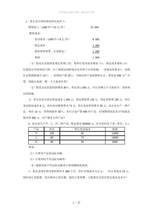
1、某企业目前的损益状况如在下:销售收入(1000件×10元/件) 10 000销售成本:变动成本(1000件×6元/件) 6 000固定成本 2 000销售和管理费(全部固定) 1 000利润 1 000(1)假设企业按国家规定普调工资,使单位变动成本增加4%,固定成本增加1%,结果将会导致利润下降。
为了抵销这种影响企业有两个应对措施:一是提高价格5%,而提价会使销量减少10%;二是增加产量20%,为使这些产品能销售出去,要追加500元广告费。
请做出选择,哪一个方案更有利?(2)假设企业欲使利润增加50%,即达到1 500元,可以从哪几个方面着手,采取相应的措施。
2、某企业每月固定制造成本1 000元,固定销售费100元,固定管理费150元;单位变动制造成本6元,单位变动销售费0.70元,单位变动管理费0.30元;该企业生产一种产品,单价10元,所得税税率50%;本月计划产销600件产品,问预期利润是多少?如拟实现净利500元,应产销多少件产品?3、某企业生产甲、乙、丙三种产品,固定成本500000元,有关资料见下表(单位:元):要求:(1)计算各产品的边际贡献;(2)计算加权平均边际贡献率;(3)根据加权平均边际贡献率计算预期税前利润。
4、某企业每年耗用某种材料3 600千克,单位存储成本为2元,一次订货成本25元。
则经济订货批量、每年最佳订货次数、最佳订货周期、与批量有关的存货总成本是多少?5.有10个同类企业的生产性固定资产年平均价值和工业总产值资料如下:(1)说明两变量之间的相关方向;(2)建立直线回归方程;(3)估计生产性固定资产(自变量)为1100万元时总产值(因变量)的可能值。
6、某商店的成本费用本期发生额如表所示,采用账户分析法进行成本估计。
首先,对每个项目进行研究,根据固定成本和变动成本的定义及特点结合企业具体情况来判断,确定它们属于哪一类成本。
例如,商品成本和利息与商店业务量关系密切,基本上属于变动成本;福利费、租金、保险、修理费、水电费、折旧等基本上与业务量无关,视为固定成本。
《数据模型与决策》复习题及参考答案

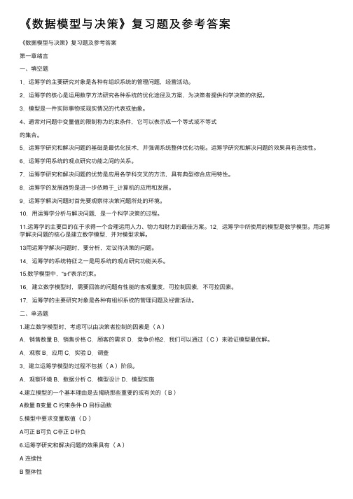
《数据模型与决策》复习题及参考答案《数据模型与决策》复习题及参考答案第一章绪言一、填空题1.运筹学的主要研究对象是各种有组织系统的管理问题,经营活动。
2.运筹学的核心是运用数学方法研究各种系统的优化途径及方案,为决策者提供科学决策的依据。
3.模型是一件实际事物或现实情况的代表或抽象。
4、通常对问题中变量值的限制称为约束条件,它可以表示成一个等式或不等式的集合。
5.运筹学研究和解决问题的基础是最优化技术,并强调系统整体优化功能。
运筹学研究和解决问题的效果具有连续性。
6.运筹学用系统的观点研究功能之间的关系。
7.运筹学研究和解决问题的优势是应用各学科交叉的方法,具有典型综合应用特性。
8.运筹学的发展趋势是进一步依赖于_计算机的应用和发展。
9.运筹学解决问题时首先要观察待决策问题所处的环境。
10.用运筹学分析与解决问题,是一个科学决策的过程。
11.运筹学的主要目的在于求得一个合理运用人力、物力和财力的最佳方案。
12.运筹学中所使用的模型是数学模型。
用运筹学解决问题的核心是建立数学模型,并对模型求解。
13用运筹学解决问题时,要分析,定议待决策的问题。
14.运筹学的系统特征之一是用系统的观点研究功能关系。
15.数学模型中,“s〃t”表示约束。
16.建立数学模型时,需要回答的问题有性能的客观量度,可控制因素,不可控因素。
17.运筹学的主要研究对象是各种有组织系统的管理问题及经营活动。
二、单选题1.建立数学模型时,考虑可以决策者控制的因素是第 1 页共40页A.销售数量B.销售价格C.顾客的需求D.竞争价格 2.我们可以通过来验证模型最优解。
A.观察B.应用C.实验D.调查 3.建立运筹学模型的过程不包括阶段。
A.观察环境B.数据分析C.模型设计D.模型实施 4.建立模型的一个基本理是去揭晓那些重要的或有关的 A数量B变量 C 约束条件 D 目标函数5.模型中要求变量取值A可正B可负C非正D非负 6.运筹学研究和解决问题的效果具有A 连续性B 整体性C 阶段性D 再生性7.运筹学运用数学方法分析与解决问题,以达到系统的最优目标。
《数据模型与决策》复习题及参考答案
《数据模型与决策》复习题及参考答案《数据模型与决策》复习题及参考答案第⼀章绪⾔⼀、填空题1.运筹学的主要研究对象是各种有组织系统的管理问题,经营活动。
2.运筹学的核⼼是运⽤数学⽅法研究各种系统的优化途径及⽅案,为决策者提供科学决策的依据。
3.模型是⼀件实际事物或现实情况的代表或抽象。
4、通常对问题中变量值的限制称为约束条件,它可以表⽰成⼀个等式或不等式的集合。
5.运筹学研究和解决问题的基础是最优化技术,并强调系统整体优化功能。
运筹学研究和解决问题的效果具有连续性。
6.运筹学⽤系统的观点研究功能之间的关系。
7.运筹学研究和解决问题的优势是应⽤各学科交叉的⽅法,具有典型综合应⽤特性。
8.运筹学的发展趋势是进⼀步依赖于_计算机的应⽤和发展。
9.运筹学解决问题时⾸先要观察待决策问题所处的环境。
10.⽤运筹学分析与解决问题,是⼀个科学决策的过程。
11.运筹学的主要⽬的在于求得⼀个合理运⽤⼈⼒、物⼒和财⼒的最佳⽅案。
12.运筹学中所使⽤的模型是数学模型。
⽤运筹学解决问题的核⼼是建⽴数学模型,并对模型求解。
13⽤运筹学解决问题时,要分析,定议待决策的问题。
14.运筹学的系统特征之⼀是⽤系统的观点研究功能关系。
15.数学模型中,“s·t”表⽰约束。
16.建⽴数学模型时,需要回答的问题有性能的客观量度,可控制因素,不可控因素。
17.运筹学的主要研究对象是各种有组织系统的管理问题及经营活动。
⼆、单选题1.建⽴数学模型时,考虑可以由决策者控制的因素是( A )A.销售数量 B.销售价格 C.顾客的需求 D.竞争价格2.我们可以通过( C )来验证模型最优解。
A.观察 B.应⽤ C.实验 D.调查3.建⽴运筹学模型的过程不包括( A )阶段。
A.观察环境 B.数据分析 C.模型设计 D.模型实施4.建⽴模型的⼀个基本理由是去揭晓那些重要的或有关的( B )A数量 B变量 C 约束条件 D ⽬标函数5.模型中要求变量取值( D )A可正 B可负 C⾮正 D⾮负6.运筹学研究和解决问题的效果具有( A )A 连续性B 整体性C 阶段性D 再⽣性7.运筹学运⽤数学⽅法分析与解决问题,以达到系统的最优⽬标。
数据、模型与决策(运筹学)课后习题和案例答案002
CHAPTER 2LINEAR PROGRAMMING: BASIC CONCEPTSReview Questions2.1-1 Ponderosa Industrial uses linear programming monthly to guide the product-mixdecision.2.1-2 Overall profitability has increased by 20%. Better utilization of raw material, capitalequipment, and personnel also resulted.2.1-3 The goal was to improve the utilization of reservation personnel by matching workschedules to customer needs.2.1-4 United Airlines saved more than $6 million annually in direct salary and benefit costs.Customer service also improved and workloads were reduced for support staff.2.1-5 The SDM system is used to coordinate the supply, distribution and marketing of eachof Citgo’s major products throughout the United States.2.1-6 Citgo saved about $14 million annually in interest expenses. Improvements incoordination, pricing, and purchasing decisions added at least $2.5 million more to annual profits.2.2-1 They provide the highest quality available in the industry for the most discriminatingbuyers.2.2-2 1) Should the company launch the two new products?2) What should be the product mix for the two new products?2.2-3 The group was asked to analyze product mix.2.2-4 Which combination of production rates for the two new products would maximize thetotal profit from both of them.2.2-5 1) available production capacity in each of the plants2) how much of the production capacity in each plant would be needed by eachproduct3) profitability of each product2.3-1 1) What are the decisions to be made?2) What are the constraints on these decisions?3) What is the overall measure of performance for these decisions?2.3-2 When formulating a linear programming model on a spreadsheet, the cells showingthe data for the problem are called the data cells. The changing cells are the cells that contain the decisions to be made. The output cells are the cells that provide output that depends on the changing cells. The target cell is a special kind of output cell that shows the overall measure of performance of the decision to be made.2.3-3 The Excel equation for each output cell can be expressed as a SUMPRODUCT function,where each term in the sum is the product of a data cell and a changing cell.2.4-1 1) Gather the relevant data.2) Identify the decisions to be made.3) Identify the constraints on these decisions.4) Identify the overall measure of performance for these decisions.5) Convert the verbal description of the constraints and measure of performance intoquantitative expressions in terms of the data and decisions2.4-2 Algebraic symbols need to be introduced to represents the measure of performanceand the decisions.2.4-3 A decision variable is an algebraic variable that represents a decision regarding thelevel of a particular activity. The objective function is the part of a linear programming model that expresses what needs to be either maximized or minimized, depending on the objective for the problem. A nonnegativity constraint is a constraint that express the restriction that a particular decision variable must be greater than or equal to zero. All constraints that are not nonnegativity constraints are referred to as functional constraints.2.4-4 A feasible solution is one that satisfies all the constraints of the problem. The bestfeasible solution is called the optimal solution.2.5-1 Two.2.5-2 The axes represent production rates for product 1 and product 2.2.5-3 The line forming the boundary of what is permitted by a constraint is called aconstraint boundary line. Its equation is called a constraint boundary equation.2.5-4 The coefficient of x1 gives the slope of the constraint boundary line. The constant termgives the value where the line intercepts the x2-axis.2.5-5 The easiest way to determine which side of the line is permitted is to check whetherthe origin (0,0) satisfies the constraint. If it does, then the permissible region lies on the side of the constraint where the origin is. Otherwise it lies on the other side.2.6-1 The Solver dialogue box.2.6-2 The Add Constraint dialogue box.2.6-3 The Assume Linear Model option and the Assume Non-Negative option.2.7-1 Cleaning products for home use.2.7-2 Television and print media.2.7-3 Determine how much to advertise in each medium to meet the market share goals ata minimum total cost.2.7-4 The changing cells are in the column for the corresponding advertising medium.2.7-5 The objective is to minimize total cost rather than maximize profit. The functionalconstraints contain ≥ rather than ≤.2.7-6 No.2.7-7 Closer to the origin.2.8-1 No.2.8-2 The graphical method helps a manager develop a good intuitive feeling for the linearprogramming is.2.8-3 1) where linear programming is applicable2) where it should not be applied3) distinguish between competent and shoddy studies using linear programming.4) how to interpret the results of a linear programming study.Problems2.1 a) The two factors that often hinder the use of optimization models by managers arecultural differences and response time. Cultural differences cause managers andmodel developers to often have a hard time understanding each other. Responsetime is often slow due to the time to translate, formulate, and solve the manger’sproblem using optimization systems.b) The company shifted from an emphasis on the manufacture of thicker plywoodsto thinner plywoods.c) Ponderosa plans to use optimization in the use of timber for other products also.In addition, optimization may be used for raw material and inventorymanagement and for financial planning.2.2 a) The shift schedules at airports and reservation offices were done by hand prior tothis study.b) The project requirements were:(i) to determine the needs for increased manpower,(ii) to identify excess manpower for reallocation,(iii) to reduce the time required for preparing schedules,(iv) to make manpower allocation more day- and time-sensitive, and(v) to quantify the cost associated with scheduling.c) Flexibility, such as the number of start times, the preferred shift lengths, the lengthof breaks, the preferred days-off combinations, etc. were considered. Thisversatility was necessary to satisfy the group culture at each office, which wasnecessary to gather field support.d) Benefits included:(i) significant labor cost savings,(ii) improved customer service,(iii) improved employee schedules,(iv) quantified manpower planning and evaluation.2.3 a) During the years preceding this study, the price of crude oil increased tenfold andshort-term interest rates more than tripled.b) Citgo’s distribution network of pipelines, tankers, and barges spanned the easterntwo-thirds of the United States. They market their products in all of the 48contiguous states.c) An 11-week planning horizon, partitioned into six one-week periods and onefive-week period, was used.d) Citgo used an IBM 4381. Typical run times for model generation, solution, andreports were two minutes, half a minute, and seven minutes, respectively.e) The four types of model users were the product managers, the pricing manager,the product traders, and the budget manager. Product managers compared the model recommendations to the actual operational decisions to determine the existence and cause of discrepancies. They also used the model's what-if capabilities to generate economically viable alternatives to current and forecasted operations. The pricing manager used the model to set ranges for terminal prices for each product and to help set prices and recommend volumes for bulk sales made to reduce excess inventories. Product traders used the model to determine which side of the trading board they should be on for each product. They also used the model's what-if capabilities to determine the sensitivity of spot prices to the required purchases or sales volumes as prices fluctuated during the week. The budget manager used the Financial Summary Report to generate various components of the monthly and quarterly budgets.f) The major reports generated by the SDM system are:(i) Infeasibility report,(ii) In-transit, Terminal, Exchange, Inventory reports, (iii) Spot recommendation report, (iv) Purchases, Sales, Trades reports, (v) Wholesale report, (vi) Volume summary report, (vii) Financial summary report.g) The education of the users was a challenge in addition to the collection, validation,and correction of input data for the model. Another challenge concerned the forecasting sales volumes and wholesales prices. Citgo forecasted for monthly and quarterly budgets, while SDM systems needed weekly forecasts.h) Direct benefits were:(i) the reduction in Citgo’s product inventory with no drop in service levels,and(ii) operational decision making improved.Indirect benefits were:(i) the establishment of a corporate database, which provided common,up-to-date, on-line, operational information for current decision, support(ii) the utilization of a single forecast throughout the different departments, which kept the entire organization, focused, (iii) the closed-loop planning process fostered by the continual feedback provided by the project manager, when comparing actual decision tomodel recommended decision, (iv) increased interdepartmental communication, and(v) the insight gained from the modeling process itself.2.4 a)b) Maximize P= $600D+ $300W,subject to D≤ 42W≤ 123D+ 2W≤ 18 and D≥ 0, W≥ 0.c) Optimal Solution = (D, W) = (x1, x2) = (4, 3). P= $3300.2.5 a) Optimal Solution: (D, W) = (x1, x2) = (1.67, 6.50). P= $3750.b) Optimal Solution: (D, W) = (x1, x2) = (1.33, 7.00). P= $3900.c) Optimal Solution: (D, W) = (x1, x2) = (1.00, 7.50). P= $4050.d) Each additional hour per week would increase total profit by $150.2.6 a)b)c)d) Each additional hour per week would increase total profit by $150.2.7a)12345678910A B C D E FP roduct A P roduct BUnit P rofit$3,000$2,000Resource ResourceUsed Available Resource Q212<=2Resource R122<=2Resource S334<=4P roduct A P roduct B Total P rofit Units P roduced0.6670.667$3,333.33Resource Usage per Unit P roducedb) Let A= units of product A producedB= units of product B produced Maximize P= $3,000A+ $2,000B, subject to 2A+ B≤ 2A+ 2B≤ 23A+ 3B≤ 4 and A≥ 0, B≥ 0.c) Optimal Solution = (A, B) = (x1, x2) = (0.667, 0.667). P= $3333.33.2.8 a) As in the Wyndor Glass Co. problem, we want to find the optimal levels of twoactivities that compete for limited resources.Let x1be the fraction purchased of the partnership in the first friends venture.Let x2 be the fraction purchased of the partnership in the second friends venture.The following table gives the data for the problem:b) The decisions to be made are how much, if any, to participate in each venture.The constraints on the decisions are that you can’t become more than a full partner in either venture, that your money is limited to $6,000, and time is limited to 600 hours. In addition, negative involvement is not possible. The overall measure of performance for the decisions is the profit to be made.c) First venture: (fraction of 1st) ≤ 1Second venture: (fraction of 2nd) ≤ 1 Money: 5000 (fraction of 1st) + 4000 (fraction of 2nd) ≤ 6000 Hours: 400 (fraction of 1st) + 500 (fraction of 2nd) ≤ 600 Nonnegativity: (fraction of 1st) ≥ 0, (fraction of 2nd) ≥ 0Profit = $4500 (fraction of 1st) + $4500 (fraction of 2nd)d)Data cells: B2:C2, B5:C6, F5:F6, and B11:C11 Changing cells: B9:C9Target cell: F9Output cells: D5:D65 6D=SU M P R ODU C T(B5:C5,$B$9:$C$9) =SU M P R ODU C T(B6:C6,$B$9:$C$9)e) This is a linear programming model because the decisions are represented bychanging cells that can have any value that satisfy the constraints. Each constraint has an output cell on the left, a mathematical sign in the middle, and a data cell on the right. The overall level of performance is represented by the target cell and the objective is to maximize that cell. Also, the Excel equation for each output cell is expressed as a SUMPRODUCT function where each term in the sum is the product of a data cell and a changing cell.f) Let x1= share taken in first friend’s venturex2= share taken in second frien d’s venture Maximize P= $4,500x1+ $4,500x2, subject to x1≤ 1 x2≤ 1$5,000x1+ $4,000x2≤ $6,000400x1+ 500x2≤ 600 hours and x1≥ 0, x2≥ 0.g) Algebraic Versiondecision variables: x1, x2functional constraints: x1≤ 1x2≤ 1$5,000x1+ $4,000x2≤ $6,000400x1+ 500x2≤ 600 hours objective function: Maximize P= $4,500x1+ $4,500x2,parameters: all of the numbers in the above algebraic modelnonnegativity constraints: x1≥ 0, x2≥ 0Spreadsheet Versiondecision variables: B9:C9functional constraints: D4:F7objective function: F9parameters: B2:C2, B5:C6, F5:F6, and B11:C11nonnegativity constraints: “Assume nonnegativity” in the Options of theSolverh) Optimal solution = (x1, x2) = (0.667, 0.667). P= $6000.2.9 a) objective function Z= x1+ 2x2functional constraints x1+ x2≤ 5x1+ 3x2≤ 9 nonnegativity constraints x1≥ 0, x2≥ 0be) 123456789A B C D E Fx1x2Unit P rofit12Resource ResourceUsed AvailableResource 1115<=5Resource 2139<=9x1x2Total P rofitDecision327Resource Usagec) Yes.d) No.f) Optimal Solution: (x1, x2) = (3, 2) and Z= 7.2.10 a) objective function Z= 3x1+ 2x2functional constraints 3x1+ x2≤ 9x1+ 2x2≤ 8 nonnegativity constraints x1≥ 0, x2≥ 0b f)1 2 3 4 5 6 7 8 9A B C D E FX1X2Unit P rofit32Resource ResourceUsed Available Resource 1319<=9 Resource 2128<=8X1X2Total P rofit Decision2312Resource Usagec) Yes.d) Yes.e) No.g & h)Optimal Solution: (x1, x2) = (2, 3) and Z= 12.2.11 a) As in the Wyndor Glass Co. problem, we want to find the optimal levels of twoactivities that compete for limited resources. We want to find the optimal mix ofthe two activities.Let W be the number of wood-framed windows to produce.Let A be the number of aluminum-framed windows to produce.The following table gives the data for the problem:Resource Usage per Unit of Activity Amount ofResource Available Resource Wood-framed Aluminum-framedGlass 6 8 48Aluminum 0 1 4Wood 1 0 6Unit Profit $60 $30b) The decisions to be made are how many windows of each type to produce. Theconstraints on the decisions are the amounts of glass, aluminum and wood available. In addition, negative production levels are not possible. The overall measure of performance for the decisions is the profit to be made.c) glass: 6 (#wood-framed) + 8 (# aluminum-framed) ≤ 48aluminum: 1 (# aluminum-framed) ≤ 4 wood: 1 (#wood-framed) ≤ 6 Nonnegativity: (#wood-framed) ≥ 0, (# aluminum-framed) ≥ 0Profit = $60 (#wood-framed) + $30 (# aluminum-framed)d)Data cells: B2:C2, B5:C5, F5, B10:C10 Changing cells: B8:C8Target cell: F8Output cells: D5, F84 5DUsed=SUM P ROD UCT(B5:C5,$B$8:$C$8)78FTotal P rofit=SUM P RODUCT(B2:C2,B8:C8)e) This is a linear programming model because the decisions are represented bychanging cells that can have any value that satisfy the constraints. Each constraint has an output cell on the left, a mathematical sign in the middle, and a data cell on the right. The overall level of performance is represented by the target cell and the objective is to maximize that cell. Also, the Excel equation for each output cell is expressed as a SUMPRODUCT function where each term in the sum is the product of a data cell and a changing cell.f) Maximize P= 60W+ 30Asubject to 6W+ 8A≤ 48 W≤ 6A≤ 4 and W≥ 0, A≥ 0.g) Algebraic Versiondecision variables: W, A functional constraints: 6W+ 8A≤ 48W≤ 6A≤ 4 objective function: Maximize P= 60W+ 30A parameters: all of the numbers in the above algebraic model nonnegativity constraints: W≥ 0, A≥ 0Spreadsheet Version decision variables: B8:C8functional constraints: D8:F8, B8:C10 objective function: F8parameters: B2:C2, B5:C5, F5, B10:C10 nonnegativity constraints: “Assume nonnegativity” in the Options of the Solverh) Optimal Solution: (W, A) = (x1, x2) = (6, 1.5) and P= $405.i) Solution unchanged when profit per wood-framed window = $40, with P = $285.Optimal Solution = (W, A) = (2.667, 4) when the profit per wood-framed window = $20, with P = $173.33.j) Optimal Solution = (W, A) = (5, 2.25) if Doug can only make 5 wood frames per day, with P = $367.50.2.12a)12345678910A B C D E F27" Sets20" SetsUnit P rofit$120$80Hours HoursUsed Available Work Hours2010500<=500Wood-fram ed Alum inum-fram ed Total P rofit Units P roduced2010$3,200<=<=4010Work Hours P er Unit P roducedb) Let x1= number of 27” TV sets to be produced per monthLet x2= number of 20” TV sets to be produced per month Maximize P= $120x1+ $80x2, subject to 20x1+ 10x2≤ 500 x1≤ 40x2≤ 10 and x1≥ 0, x2≥ 0.c) Optimal Solution: (x1, x2) = (20, 10) and P= $3200.2.13 a) If x2 = 0 then x1 = 2. If x1 = 0 then x2 = 4.b)c) slope = –2d) x2 = -2x1 + 4, slope = –2, x2-intercept = 42.14 a) If x2 = 0 then x1 = 5. If x1 = 0 then x2 = 2.b)c) slope = –0.4d) x2 = –0.4x1 + 2, slope = –0.4, x2 intercept = 22.15 a) If x2 = 0 then x1 = 6. If x1 = 0 then x2 = –4.b)c) slope = 0.667d) x2 = 0.667x1– 4, slope = 0.667, x2 intercept = –42.16 a)b)c)d)2.17 a)b)c)d)2.18 a)b)c)d)2.19 a) The decisions to be made are how many of each light fixture to produce. Theconstraints are the amounts of frame parts and electrical components available,and the maximum number of product 2 that can be sold (60 units). In addition,negative production levels are not possible. The overall measure of performancefor the decisions is the profit to be made.b) frame parts: 1 (# product 1) + 3 (# product 2) ≤ 200electrical components: 2 (# product 1) + 2 (# product 2) ≤ 300 product 2 max.: 1 (# product 2) ≤ 60 Nonnegativity: (# product 1) ≥ 0, (# product 2) ≥ 0Profit = $1 (# product 1) + $2 (# product 2)c)1234567891011A B C D E FP roduct 1P roduct 2Unit P rofit$1$2Resource ResourceUsed AvailableFram e P arts13200<=200E lectrical Com ponents22300<=300P roduct 1P roduct 2Total P rofitP roduction12525$175<=60Resource Usaged) Let x1= number of units of product 1 to producex2= number of units of product 2 to produce Maximize P= $1x1+ $2x2, subject to x1+ 3x2≤ 200 2x1+ 2x2≤ 300x2≤ 60 and x1≥ 0, x2≥ 0.e) Optimal Solution: (x1, x2) = (125, 25) and P= $175.2.20 a) The decisions to be made are what quotas to establish for the two product lines.The constraints are the amounts of work hours available in underwriting,administration, and claims. In addition, negative levels are not possible. Theoverall measure of performance for the decisions is the profit to be made.b) underwriting: 3 (# special risk) + 2 (# mortgage) ≤ 2400administration: 1 (# mortgage) ≤ 800claims: 2 (# special risk) ≤ 1200Nonnegativity: (# special risk) ≥ 0, (# mortgage) ≥ 0Profit = $5 (# special risk) + $2 (# mortgage)c)d) Let S= units of special risk insuranceM= units of mortgages Maximize P= $5S+ $2M,subject to 3S+ 2M≤ 2,400M≤ 8002S≤ 1,200 and S≥ 0, M≥ 0.e) Optimal Solution: (S, M) = (x1, x2) = (600, 300) and P= $3600.2.21 a)P=6 P=12 P=18b)slope-intercept form slope x2 interceptP=6 x2 = –0.667x1 + 2 –0.667 2P=12 x2 = –0.667x1 + 4 –0.667 4P=18 x2 = –0.667x1 + 6 –0.667 62.22 a)P=100 P=200 P=300b)slope-intercept form slope x2 intercept P=100 x2 = -2.5x1 + 10 –2.5 10P=200 x2 = -2.5x1 + 20 –2.5 20P=300 x2 = -2.5x1 + 30 –2.5 302.23 a) Cost=100 200 300b)slope-intercept form slope x2 intercept C=300 x2 = 5x1– 300 5 –300C=200 x2 = 5x1– 200 5 –200C=100 x2 = 5x1– 100x2 5 –100 2.24 a) x2 = –0.5x1 + 10b) slope = –0.5, x2-intercept = 10c)2.25 x2 = –1.6x1 + 82.26 a) x2 = –2x1 + 4b) x2 = 0.667x1 + 2c) x2 = 2.5x1– 52.27 a) x1– 2x2 = 0b) x2 = 0.5x1c) slope = 0.5, x2-intercept = 0d)e) The area above the constraint boundary line is permitted by the constraint.2.28 a) Optimal Solution: (x1, x2) = (0, 7) and Z=70.b)123456789A B C D E FX1X2Unit P rofit2010Resource ResourceUsed AvailableResource 11-1-7<=1Resource 2317<=7X1X2Total P rofitDecision0770Resource Usage2.29 a) Optimal Solution: (x1, x2) = (13, 5) and P= 31.b)1 2 3 4 5 6 7 8 9 10 11A B C D E FX1X2Unit P rofit21Resource ResourceUsed Available Resource 1015<=10 Resource 22551<=60 Resource 31118<=18 Resource 43144<=44X1X2Total P rofit Decision13531Resource Usage2.30 a) Optimal Solution: (x1, x2) = (2, 6) and P= 18.b)1 2 3 4 5 6 7 8 9A B C D E FP roduct 1P roduct 2Unit P rofit32Resource ResourceUsed Available Resource 1118<=8 Resource 22110<=10P roduct 1P roduct 2Total P rofit Decision2618Resource Usage2.31 a) Optimal Solution: (x1, x2) = (3, 9) and P=210.b)12345678910A B C D E FActivity 1Activity 2Unit P rofit1020Resource ResourceUsed AvailableResource 1-1215<=15Resource 21112<=12Resource 35342<=45Activity 1Activity 2Total P rofitDecision39210Resource Usage2.32 a & b)Optimal Solution: (x1, x2) = (3.333, 3.333) and P = 3000.2.33 a) The decisions to be made are how many hotdogs and buns should be produced.The constraints are the amounts of flour and pork available, and the hoursavailable to work. In addition, negative production levels are not possible. Theoverall measure of performance for the decisions is the profit to be made.b) flour: 0.1 (# buns) ≤ 200pork: 0.25 (# hotdogs) ≤ 800work hours: 3 (# hotdogs) + 2 (# buns) ≤ 12,000Nonnegativity: (# hotdogs) ≥ 0, (# buns) ≥ 0Profit = 0.2 (# hotdogs) + 0.1 (# buns)c)d) Let H= # of hot dogs to produceB= # of buns to produce Maximize P= $0.20H+ $0.10B,subject to 0.1B≤ 2000.25H≤ 8003H+ 2B≤ 12,000 and H≥ 0, B≥ 0.e) Optimal Solution: (H, B) = (x1, x2) = (3200, 1200) and P=$760.2.34 a)1 2 3 4 5 6 7 8 9 10 11 12A B C D E FTables ChairsUnit P rofit$400$100Resource ResourceUsed Available Oak50252,500<=2,500 Labor Hours66450<=480Tables Chairs Total P rofit Decision2550$15,000Chairs50>=502Times Numberof TablesResource Usageb) Let T= # of tables to produceC= # of chairs to produce Maximize P= $400T+ $100C subject to 50T+ 25C≤ 2,500 6T+ 6C≤ 480C≥ 2T and T≥ 0, C≥ 0.c) Optimal Solution: (T, C) = (x¡, x2) = (25, 50) and P=$15,000.2.35 a)1 2 3 4 5 6 7 8 9 10 11 12 13 14 15 16 17 18A B C D E F G H I J KBeef Gravy P eas Carrots RollUnit Cost$0.40$0.35$0.15$0.18$0.10(per ounce)Nutritional Data (per ounce)Total in Diet Needed Maximum Calories542015840320>=280<=320 Fat Calories1915001096Vitamin A (IU)00153500600>=600Vitamin C (m g)0131012.38>=10 P rotein (g)8011130>=30Beef Gravy P eas Carrots Roll Total CostDiet (ounces) 2.94 1.47 3.11 1.58 1.82$2.62>=Minimums2Fat Calories96<=9630%of Total CaloriesGravy 1.47>= 1.4750%of Beefb) Let B = ounces of beef tips in diet,G = ounces of gravy in diet,P = ounces of peas in diet,C = ounces of carrots in diet,R = ounces of roll in diet.Minimize Z= $0.40B+ $0.35G+ $0.15P+ $0.18C+ $0.10R subject to 54B+ 20G+ 15P+ 8C+ 40R≥ 280 54B+ 20G+ 15P+ 8C+ 40R≤ 32019B+ 15G+ 10R≤ 0.3(54B+ 20G+ 15P+ 8C+ 40R)15P+ 350C≥ 600G+ 3P+ C≥ 108B+ P+ C+ R≥ 30B≥ 2G≥ 0.5B and B≥ 0, G≥ 0, P≥ 0, C≥ 0, R≥ 0.2.36 When c< 0.5, the optimal solution is (x1, x2) = (0, 5).When c = 0.5, the optimal solutions are (x1, x2) = (0, 5), (2, 4), and all points on the connecting line.When 0.5 < c< 1, the optimal solution is (x1, x2) = (2, 4).When c= 1, the optimal solutions are (x1, x2) = (6, 0), (2, 4), and all points on the connecting line.When c> 1, the optimal solution is (x1, x2) = (6, 0).2.37 When c< –2, the optimal solution is (x1, x2) = (2, 0).When c = –2, the optimal solutions are (x1, x2) = (2, 0), (2.8, 0.8), and all points on the connecting line.When –2 < c< 8, the optimal solution is (x1, x2) = (2.8, 0.8).When c = 8, the optimal solutions are (x1, x2) = (3, 0), (2.8, 0.8), and all points on the connecting line.When c> 8, the optimal solution is (x1, x2) = (3, 0).2.38 When k < 0.5 (for example, k = 0.25 is graphed below), the optimal solution is (x1, x2)= ([2k+3]/k, 0). Thus, (2, 30) is not optimal for these values of k.When k≥ 0.5 (for example, k = 1 is graphed below), the optimal solution is (x1, x2) = (2, 3).2.39 a) The decisions to be made are how many servings of steak and potatoes areneeded. The constraints are the amounts of carbohydrates, protein, and fat thatare needed. In addition, negative levels are not possible. The overall measure ofperformance for the decisions is the cost.b) carbohydrates: 5 (# steak) + 15 (# potatoes) ≥ 50protein: 20 (# steak) + 5 (# potatoes) ≥ 40 fat: 15 (# steak) + 2 (# potatoes) ≤ 60 Nonnegativity: (# steak) ≥0, (# potatoes) ≥ 0Cost = 4 (# steak) + 2 (# potatoes)c)12345678910A B C D E FSteak P otatoesUnit C ost$4$2Total Nutrition Daily Requirem ent(gram s)(gram s) Carbohydrates51550>=50P rotein20540>=40Fat15224.91<=60Steak P otatoes Total CostServings 1.27 2.91$10.91Nutritional Info (gram s/serving)d) Let S= servings of steak in dietP= servings of potatoes in the diet Minimize C= $4S+ $2P, subject to 5S+ 15P≥ 50 20S+ 5P≥ 4015S+ 2P≤ 60 and S≥ 0, P≥ 0.e & f) Optimal Solution: (S, P) = (x1, x2) = (1.27, 2.91) and C= $10.91.2.40 a) Optimal solution: (x1, x2) = (2, 4) and C=110.b)1 2 3 4 5 6 7 8 9 10A B C D E FActivity 1Activity 2Unit Cost1520Total Lim it Constraint 11210>=10 Constraint 22-3-8<=6 Constraint 3116>=6Activity 1Activity 2Total Cost Decision241102.41 a) The decisions to be made are what combination of feed types to use. Theconstraints are the amounts of calories and vitamins needed, and a maximumlevel for feed type A. In addition, negative levels are not possible. The overallmeasure of performance for the decisions is the cost.b) Calories: 800 (lb. Type A) + 1000 (lb. Type B) ≥ 8000Vitamins: 140 (lb. Type A) + 70 (lb. Type B) ≥ 700Type A maximum: (lb. Type A) ≤ 0.333((lb. Type A) + (lb. Type B))Nonnegativity: (lb. Type A) ≥ 0, (lb. Type B) ≥ 0Cost = $0.40 (lb. Type A) + $0.80 (lb. Type B)c)1234567891011A B C D E FFeed A Feed BUnit Cost$0.40$0.80(per pound)Total DailyNutrition Requirem entCalories8001,0008,000>=8,000Vitam ins14070800>=700Feed A Feed B Total CostDiet (pounds) 2.86 5.71$5.71<=2.8633.33%of Total DietNutrition (per pound)d) Let A= pounds of Feed Type A in dietB= pounds of Feed Type B in diet Minimize C= $0.40A+ $0.80B, subject to 800A+ 1,000B≥ 8,000 140A+ 70B≥ 700A≤ (1/3)(A+ B) and A≥ 0, B≥ 0.e) Optimal Solution: (A, B) = (x1, x2) = (2.86, 5.71) and C= $5.72.。
运筹学数据模型与决策教材习题答案
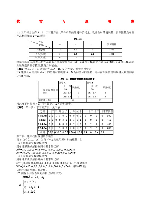
教材习题答案1.2 工厂每月生产A 、B 、C 三种产品 ,单件产品的原材料消耗量、设备台时的消耗量、资源限量及单件产品利润如表1-22所示.130.试建立该问题的数学模型,使每月利润最大.【解】设x 1、x 2、x 3分别为产品A 、B 、C 的产量,则数学模型为1.3 建筑公司需要用6m 长的塑钢材料制作A 、B 两种型号的窗架.两种窗架所需材料规格及数量如表1-23所示:【解】 设x j (j =1,2,…,14)为第j 种方案使用原材料的根数,则 (1)用料最少数学模型为用单纯形法求解得到两个基本最优解X (1)=( 50 ,200 ,0 ,0,84 ,0,0 ,0 ,0 ,0 ,0 ,200 ,0 ,0 );Z=534 X (2)=( 0 ,200 ,100 ,0,84 ,0,0 ,0 ,0 ,0 ,0 ,150 ,0 ,0 );Z=534 (2)余料最少数学模型为用单纯形法求解得到两个基本最优解X (1)=( 0 ,300 ,0 ,0,50 ,0,0 ,0 ,0 ,0 ,0 ,200 ,0 ,0 );Z=0,用料550根 X (2)=( 0 ,450 ,0 ,0,0 ,0,0 ,0 ,0 ,0 ,0 ,200 ,0 ,0 );Z=0,用料650根 显然用料最少的方案最优。
1.7 图解下列线性规划并指出解的形式:(1) 121212max 2131,0Z x x x x x x x x =-++≥⎧⎪-≥-⎨⎪≥⎩【解】最优解X =(1/2,1/2);最优值Z=-1/2(2) 12121212min 32223120,0Z x x x x x x x x =---≥-⎧⎪+≤⎨⎪≥≥⎩【解】最优解X =(3/4,7/2);最优值Z=-45/4(3)121212121212min 322114102731,0Z x x x x x x x x x x x x =-++≤⎧⎪-+≤⎪⎪-≤⎨⎪-≤⎪⎪≥⎩【解】最优解X =(4,1);最优值Z=-10(4) 121212112max 3812223,0Z x x x x x x x x x =++≤⎧⎪+≤⎪⎨≤⎪⎪≥⎩ 【解】最优解X =(3/2,1/4);最优值Z=7/4(5) ⎪⎪⎩⎪⎪⎨⎧≥≤≥≥-+=0,6322min 21212121x x x x x x x x Z 【解】最优解X =(3,0);最优值Z=3 (6) ⎪⎪⎩⎪⎪⎨⎧≥≤≥≥-+=0,6322max 21212121x x x x x x x x Z【解】无界解。
《数据模型与决策》复习题及参考答案
《数据模型与决策》复习题及参考答案一、填空题1.运筹学的主要研究对象是各种有组织系统的管理问题,经营活动。
2.运筹学的核心是运用数学方法研究各种系统的优化途径及方案,为决策者提供科学决策的依据。
3.模型是一件实际事物或现实情况的代表或抽象。
4、通常对问题中变量值的限制称为约束条件,它可以表示成一个等式或不等式的集合。
5.运筹学研究和解决问题的基础是最优化技术,并强调系统整体优化功能。
运筹学研究和解决问题的效果具有连续性。
6.运筹学用系统的观点研究功能之间的关系。
7.运筹学研究和解决问题的优势是应用各学科交叉的方法,具有典型综合应用特性。
8.运筹学的发展趋势是进一步依赖于_计算机的应用和发展。
9.运筹学解决问题时首先要观察待决策问题所处的环境。
10.用运筹学分析与解决问题,是一个科学决策的过程。
11.运筹学的主要目的在于求得一个合理运用人力、物力和财力的最佳方案。
12.运筹学中所使用的模型是数学模型。
用运筹学解决问题的核心是建立数学模型,并对模型求解。
13用运筹学解决问题时,要分析,定议待决策的问题。
14.运筹学的系统特征之一是用系统的观点研究功能关系。
15.数学模型中,“s·t”表示约束。
16.建立数学模型时,需要回答的问题有性能的客观量度,可控制因素,不可控因素。
17.运筹学的主要研究对象是各种有组织系统的管理问题及经营活动。
二、单选题1.建立数学模型时,考虑可以由决策者控制的因素是(A)A.销售数量B.销售价格C.顾客的需求D.竞争价格2.我们可以通过(C)来验证模型最优解。
A.观察B.应用C.实验D.调查3.建立运筹学模型的过程不包括(A)阶段。
A.观察环境B.数据分析C.模型设计D.模型实施4.建立模型的一个基本理由是去揭晓那些重要的或有关的(B)A数量B变量C约束条件D目标函数5.模型中要求变量取值(D)A可正B可负C非正D非负6.运筹学研究和解决问题的效果具有(A)A连续性B整体性C阶段性D再生性7.运筹学运用数学方法分析与解决问题,以达到系统的最优目标。
《数据模型与决策》复习题及参考答案

《数据模型与决策》复习题及参考答案《数据模型与决策》复习题及参考答案第⼀章绪⾔⼀、填空题1.运筹学的主要研究对象是各种有组织系统的管理问题,经营活动。
2.运筹学的核⼼是运⽤数学⽅法研究各种系统的优化途径及⽅案,为决策者提供科学决策的依据。
3.模型是⼀件实际事物或现实情况的代表或抽象。
4、通常对问题中变量值的限制称为约束条件,它可以表⽰成⼀个等式或不等式的集合。
5.运筹学研究和解决问题的基础是最优化技术,并强调系统整体优化功能。
运筹学研究和解决问题的效果具有连续性。
6.运筹学⽤系统的观点研究功能之间的关系。
7.运筹学研究和解决问题的优势是应⽤各学科交叉的⽅法,具有典型综合应⽤特性。
8.运筹学的发展趋势是进⼀步依赖于_计算机的应⽤和发展。
9.运筹学解决问题时⾸先要观察待决策问题所处的环境。
10.⽤运筹学分析与解决问题,是⼀个科学决策的过程。
11.运筹学的主要⽬的在于求得⼀个合理运⽤⼈⼒、物⼒和财⼒的最佳⽅案。
12.运筹学中所使⽤的模型是数学模型。
⽤运筹学解决问题的核⼼是建⽴数学模型,并对模型求解。
13⽤运筹学解决问题时,要分析,定议待决策的问题。
14.运筹学的系统特征之⼀是⽤系统的观点研究功能关系。
15.数学模型中,“s〃t”表⽰约束。
16.建⽴数学模型时,需要回答的问题有性能的客观量度,可控制因素,不可控因素。
17.运筹学的主要研究对象是各种有组织系统的管理问题及经营活动。
⼆、单选题1.建⽴数学模型时,考虑可以由决策者控制的因素是( A )A.销售数量 B.销售价格 C.顾客的需求 D.竞争价格2.我们可以通过( C )来验证模型最优解。
A.观察 B.应⽤ C.实验 D.调查3.建⽴运筹学模型的过程不包括( A )阶段。
A.观察环境 B.数据分析 C.模型设计 D.模型实施4.建⽴模型的⼀个基本理由是去揭晓那些重要的或有关的( B )A数量 B变量 C 约束条件 D ⽬标函数5.模型中要求变量取值( D )A可正 B可负 C⾮正 D⾮负6.运筹学研究和解决问题的效果具有( A )A 连续性B 整体性C 阶段性D 再⽣性7.运筹学运⽤数学⽅法分析与解决问题,以达到系统的最优⽬标。
《数据、模型与决策》习题
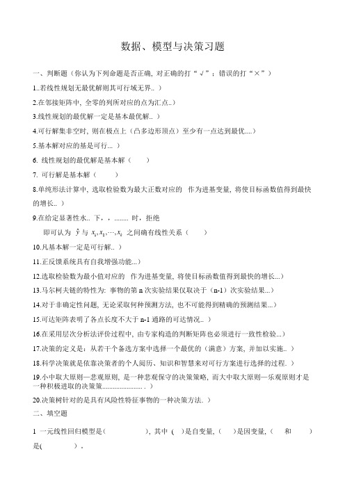
数据、模型与决策习题一、判断题(你认为下列命题是否正确, 对正确的打“√”;错误的打“×”) 1..若线性规划无最优解则其可行域无界.. ) 2.在邻接矩阵中, 全零的列所对应的点为汇点..) 3.线性规划的最优解一定是基本最优解.. )4.可行解集非空时, 则在极点上(凸多边形顶点)至少有一点达到最优....)5.基本解对应的基是可行... )6. 线性规划的最优解是基本解( )7. 可行解是基本解( )8.单纯形法计算中, 选取检验数为最大正数对应的 作为进基变量, 将使目标函数值得到最快的增长.. )9.在给定显著性水.. 下,,........ 时,拒绝即可认为 与 之间确有线性关系( ) 10.凡基本解一定是可行解.. ) 11.正反馈系统具有自我增强功能...)12.选取检验数为最小值对应的 作为进基变量, 将使目标函数值得到最快的增长...) 13.马尔柯夫链的特性为: 事物的第n 次实验结果仅取决于(n-1)次实验结果...) 14.对于非确定性问题, 无论采取何种预测方法, 也不可能得到精确的预测结果...) 15.可达矩阵表明了各点长度不大于n-1通路的可达情况.. )16.在采用层次分析法评价过程中, 由专家构造的判断矩阵也必须进行一致性检验...) 17.决策的定义是:从若干个备选方案中选择一个最优的(满意)方案, 并加以实施.. ) 18.科学决策就是依靠决策者的个人阅历、知识和智慧来对可行方案进行选择的过程. ) 19.小中取大原则—悲观原则, 是一种悲观保守的决策策略, 而大中取大原则—乐观原则才是一种积极进取的决策策....................... . )20.决策树针对的是具有风险性特征事物的一种决策方法. ) 二、填空题1 一元线性回归模型是( ), 其中 ( )是自变量, ( )是因变量, ( 和 )是( )。
y ˆk x x x ,,,212 由 , 得出 , , 其中 等于( ), 等于( ), 则用于一元线性回归模型 , 表示为( )。
《数据模型与决策》练习题及答案
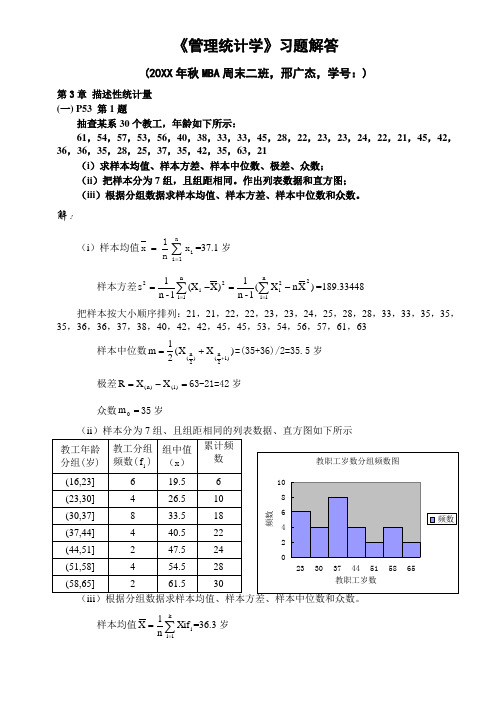
《管理统计学》习题解答(20XX 年秋MBA 周末二班,邢广杰,学号:)第3章 描述性统计量 (一) P53 第1题抽查某系30个教工,年龄如下所示:61,54,57,53,56,40,38,33,33,45,28,22,23,23,24,22,21,45,42,36,36,35,28,25,37,35,42,35,63,21(i )求样本均值、样本方差、样本中位数、极差、众数;(ii )把样本分为7组,且组距相同。
作出列表数据和直方图; (iii )根据分组数据求样本均值、样本方差、样本中位数和众数。
解:(i )样本均值∑==n1i ixn1x =37.1岁样本方差)X n X (1-n 1)X (X 1-n 1s 2n 1i 2i2n 1i i 2-=-=∑∑===189.33448 把样本按大小顺序排列:21,21,22,22,23,23,24,25,28,28,33,33,35,35,35,36,36,37,38,40,42,42,45,45,53,54,56,57,61,63样本中位数)X X (21m 1)2n ()2n (++==(35+36)/2=35.5岁极差=-=1)()n (X X R 63-21=42岁 众数=0m 35岁(ii )样本分为7组、且组距相同的列表数据、直方图如下所示样本均值i k1i f Xi n 1X ∑===36.3岁样本方差)X n f X (1-n 1f )X (X 1-n 1s 2k 1i i 2i i2k 1i i 2-=-=∑∑===174.3724 样本中位数810230730f F 2n i I m -+=-+==34.375岁 众数=--⨯-+=---+=+448248730f f 2f f f iI m 1m 1-m m 1-m m 033.5岁(二)P53 第2题某单位统计了不同级别的员工的月工资水平资料如下:解:样本均值i k1i f Xi n 1X ∑===1566.667元样本标准差)X n f X (1-n 1f )X (X 1-n 1s 2k 1i i2i i 2k 1i i -=-=∑∑===398.1751元 样本中位数在累计74人的那一组,m=1500元; 众数1500m 0=元。
《数据模型与决策》复习题及参考答案0

《数据模型与决策》复习题及参考答案0《数据模型与决策》复习题及参考答案⼀、填空题1.运筹学的主要研究对象是各种有组织系统的管理问题,经营活动。
2.运筹学的核⼼主要是运⽤数学⽅法研究各种系统的优化途径及⽅案,为决策者提供科学决策的依据。
3.模型是⼀件实际事物或现实情况的代表或抽象。
4通常对问题中变量值的限制称为约束条件,它可以表⽰成⼀个等式或不等式的集合。
5.运筹学研究和解决问题的基础是最优化技术,并强调系统整体优化功能。
运筹学研究和解决问题的效果具有连续性。
6.运筹学⽤系统的观点研究功能之间的关系。
7.运筹学研究和解决问题的优势是应⽤各学科交叉的⽅法,具有典型综合应⽤特性。
8.运筹学的发展趋势是进⼀步依赖于_计算机的应⽤和发展。
9.运筹学解决问题时⾸先要观察待决策问题所处的环境。
10.⽤运筹学分析与解决问题,是⼀个科学决策的过程。
11.运筹学的主要⽬的在于求得⼀个合理运⽤⼈⼒、物⼒和财⼒的最佳⽅案。
12.运筹学中所使⽤的模型是数学模型。
⽤运筹学解决问题的核⼼是建⽴数学模型,并对模型求解。
13⽤运筹学解决问题时,要分析,定议待决策的问题。
14.运筹学的系统特征之⼀是⽤系统的观点研究功能关系。
15.数学模型中,“s·t”表⽰约束。
16.建⽴数学模型时,需要回答的问题有性能的客观量度,可控制因素,不可控因素。
17.运筹学的主要研究对象是各种有组织系统的管理问题及经营活动。
⼆、单选题1.建⽴数学模型时,考虑可以由决策者控制的因素是( A )A.销售数量 B.销售价格 C.顾客的需求 D.竞争价格2.我们可以通过( C )来验证模型最优解。
A.观察 B.应⽤ C.实验 D.调查3.建⽴运筹学模型的过程不包括( A )阶段。
A.观察环境 B.数据分析 C.模型设计 D.模型实施4.建⽴模型的⼀个基本理由是去揭晓那些重要的或有关的( B )A数量 B变量 C 约束条件 D ⽬标函数5.模型中要求变量取值( D )A可正 B可负 C⾮正 D⾮负6.运筹学研究和解决问题的效果具有( A )A 连续性B 整体性C 阶段性D 再⽣性7.运筹学运⽤数学⽅法分析与解决问题,以达到系统的最优⽬标。
《数据模型与决策》复习试题和参考题答案

《数据模型与决策》复习题及参考答案第一章绪言一、填空题1.运筹学的主要研究对象是各种有组织系统的管理问题,经营活动。
2.运筹学的核心是运用数学方法研究各种系统的优化途径及方案,为决策者提供科学决策的依据。
3.模型是一件实际事物或现实情况的代表或抽象。
4、通常对问题中变量值的限制称为约束条件,它可以表示成一个等式或不等式的集合。
5.运筹学研究和解决问题的基础是最优化技术,并强调系统整体优化功能。
运筹学研究和解决问题的效果具有连续性。
6.运筹学用系统的观点研究功能之间的关系。
7.运筹学研究和解决问题的优势是应用各学科交叉的方法,具有典型综合应用特性。
8.运筹学的发展趋势是进一步依赖于_计算机的应用和发展。
9.运筹学解决问题时首先要观察待决策问题所处的环境。
10.用运筹学分析与解决问题,是一个科学决策的过程。
11.运筹学的主要目的在于求得一个合理运用人力、物力和财力的最佳方案。
12.运筹学中所使用的模型是数学模型。
用运筹学解决问题的核心是建立数学模型,并对模型求解。
13用运筹学解决问题时,要分析,定议待决策的问题。
14.运筹学的系统特征之一是用系统的观点研究功能关系。
15.数学模型中,“s·t”表示约束。
16.建立数学模型时,需要回答的问题有性能的客观量度,可控制因素,不可控因素。
17.运筹学的主要研究对象是各种有组织系统的管理问题及经营活动。
二、单选题1.建立数学模型时,考虑可以由决策者控制的因素是( A )A.销售数量 B.销售价格 C.顾客的需求 D.竞争价格2.我们可以通过( C )来验证模型最优解。
A.观察 B.应用 C.实验 D.调查3.建立运筹学模型的过程不包括( A )阶段。
A.观察环境 B.数据分析 C.模型设计 D.模型实施4.建立模型的一个基本理由是去揭晓那些重要的或有关的( B )A数量 B变量 C 约束条件 D 目标函数5.模型中要求变量取值( D )A可正 B可负 C非正 D非负6.运筹学研究和解决问题的效果具有( A )A 连续性B 整体性C 阶段性D 再生性7.运筹学运用数学方法分析与解决问题,以达到系统的最优目标。
数据、模型与决策(运筹学)课后习题和案例答案005
CHAPTER 5 WHAT-IF ANALYSIS FOR LINEAR PROGRAMMINGReview Questions5.1-1 The parameters of a linear programming model are the constants (coefficients or right-handsides) in the functional constraints and the objective function.5.1-2 Many of the parameters of a linear programming model are only estimates of quantities thatcannot be determined precisely and thus result in inaccuracies.5.1-3 What-if analysis reveals how close each of these estimates needs to be to avoid obtainingan erroneous optimal solution, and therefore pinpoints the sensitive parameters where extra care is needed to refine their estimates.5.1-4 No, if the optimal solution will remain the same over a wide range of values for a particularcoefficient, then it may be appropriate to make only a fairly rough estimate for a parameter of a model.5.1-5 Conditions that impact the parameters of a model, such as unit profit, may change over timeand render them inaccurate.5.1-6 If conditions change, what-if analysis leaves signposts that indicate whether a resultingchange in a parameter of the model changes the optimal solution.5.1-7 Sensitivity analysis is studying how changes in the parameters of a linear programmingmodel affect the optimal solution.5.1-8 What-if analysis provides guidance about what the impact would be of altering policydecisions that are represented by parameters of a model.5.2-1 The estimates of the unit profits for the two products are most questionable.5.2-2 The number of hours of production time that is being made available per week in the threeplants might change after analysis.5.3-1 The allowable range for a coefficient in the objective function is the range of values overwhich the optimal solution for the original model remains optimal.5.3-2 If the true value for a coefficient in the objective function lies outside its allowable rangethen the optimal solution would change and the problem would need to be resolved.5.3-3 The Objective Coefficient column gives the current value of each coefficient. TheAllowable Increase column and the Allowable Decrease Column give the amount that each coefficient may differ from these values to remain within the allowable range for which the optimal solution for the original model remains optimal.5.4-1 The 100% rule considers the percentage of the allowable change (increase or decrease) foreach coefficient in the objective function.5.4-2 If the sum of the percentage changes do not exceed 100% then the original optimal solutiondefinitely will still be optimal.5.4-3 No, exceeding 100% may or may not change the optimal solution depending on thedirections of the changes in the coefficients.5.5-1 The parameters in the constraints may only be estimates, or, especially for the right-hand-sides, may well represent managerial policy decisions.5.5-2 The right-hand sides of the functional constraints may well represent managerial policydecisions rather than quantities that are largely outside the control of management.5.5-3 The shadow price for a functional constraint is the rate at which the value of the objectivefunction can be increased by increasing the right-hand side of the constraint by a smallamount.5.5-4 The shadow price can be found with the spreadsheet by increasing the right-hand side byone, and then re-solving to determine the increase in the objective function value. It can be found similarly with a Solver Table by creating a table that shows the increase in profit fora unit increase in the right-hand side. The shadow price is given directly in the sensitivityreport.5.5-5 The shadow price for a functional constraint informs management about how much thetotal profit will increase for each extra unit of a resource (right-hand-side of a constraint).5.5-6 Yes. The shadow price also indicates how much the value of the objective function willdecrease if the right-hand side were to be decreased by 1.5.5-7 A shadow price of 0 tells a manager that a small change in the right-hand side of theconstraint will not change the objective function value at all.5.5-8 The allowable range for the right-hand side of a functional constraint is found in theSolver’s sensitivity report by using the columns labeled “Constraint R.H. Side”,“Allowable increase”, and “Allowable decrease”.5.5-9 The allowable ranges for the right-hand sides are of interest to managers because they tellthem how large changes in the right-hand sides can be before the shadow prices are nolonger applicable.5.6-1 There may be uncertainty about the estimates for a number of the parameters in thefunctional constraints. Also, the right-hand sides of the constraints often representmanagerial policy decisions. These decisions are frequently interrelated and so need to beconsidered simultaneously.5.6-2 The spreadsheet can be used to directly determine the impact of several simultaneouschanges. Simply change the paremeters and re-solve.5.6-3 Using Solver Table, trial values can be enumerated simultaneously for one or two data cells,with the possibility of entering formulas for additional data cells in terms of these one ortwo data cells.5.6-4 The right-hand sides of the constraints often represent managerial policy decisions. Thesedecisions are frequently interrelated and so need to be considered simultaneously.5.6-5 The 100 percent rule basically says that we can safely use the shadow prices to predict theeffect of simultaneous changes in the right-hand sides if the sum of the percentages of the changes does not exceed 100 percent.5.6-6 The data needed to apply the 100% rule for simultaneous changes in right-hand sides aregiven by the Sensitivity Report (Constraint R.H. Side, Allowable Increase, and Allowable Decrease).5.6-7 If the sum of the percentage changes does not exceed 100%, the shadow prices definitelywill still be valid.5.6-8 If the sum of the percentages of allowable changes in the right-hand sides does exceed100%, then we cannot be sure if the shadow prices will still be valid.Problems5.1 a)b)The estimate of the unit profit for toys can decrease by somewhere between $0 and$0.50 before the optimal solution will change. There is no change in the solution for anincrease in the unit profit for toys (at least for increase up to $1).c)The estimate of the unit profit for subassemblies can decrease by somewhere between $0 and $0.50 before the optimal solution will change. There is no change in the solution for an increase in the unit profit for subassemblies (at least for increases up to $1).d) Solver Table for change in unit profit for toys (part b):11 12 13 14 15 16 17 18 19 20 21 22A B C D Unit P rofitfor Toys Toys Subassem blies Total P rofit2,0001,000$3,500 $2.0010000$2,000 $2.2510000$2,250 $2.5010000$2,500 $2.7520001000$3,000 $3.0020001000$3,500 $3.2520001000$4,000 $3.5020001000$4,500 $3.7520001000$5,000 $4.0020001000$5,500P roductionSolver Table for change in unit profit for subassemblies (part c):11 12 13 14 15 16 17 18 19 20 21 22A B C DUnit P rofitfor Subassem blies Toys Subassem blies Total P rofit2,0001,000$3,500 -$3.5010000$3,000-$3.2510000$3,000-$3.0010000$3,000-$2.7520001000$3,250-$2.5020001000$3,500-$2.2520001000$3,750-$2.0020001000$4,000-$1.7520001000$4,250-$1.5020001000$4,500P roductione) The unit profit for toys can vary between $2.50 and $5.00 before the solution changes.The unit profit for subassemblies can vary between (–$3.00) and (–$1.50) before the solution changes.f) The allowable range for the unit profit for toys is $2.50 to $5.00.The allowable range for the unit profit for subassemblies as (–$3.00) to (–$1.50).Adjustable CellsFinal Reduced Objective Allowable Allowable Cell Name Value Cost CoefficientIncreaseDecrease$B$9P roduction Toys2,0000320.5$C$9P roduction Subassem blies1,000-2.510.5g)1112131415161718192021AB C D E F G H I J K Total P rofitUnit P rofit for Subassem blies $3,500-$3.50-$3.25-$3.00-$2.75-$2.50-$2.25-$2.00-$1.75-$1.50$2.00$2,000$2,000$2,000$2,000$2,000$2,000$2,000$2,250$2,500$2.25$2,250$2,250$2,250$2,250$2,250$2,250$2,500$2,750$3,000$2.50$2,500$2,500$2,500$2,500$2,500$2,750$3,000$3,250$3,500Unit P rofit $2.75$2,750$2,750$2,750$2,750$3,000$3,250$3,500$3,750$4,000for Toys$3.00$3,000$3,000$3,000$3,250$3,500$3,750$4,000$4,250$4,500$3.25$3,250$3,250$3,500$3,750$4,000$4,250$4,500$4,750$5,000$3.50$3,500$3,750$4,000$4,250$4,500$4,750$5,000$5,250$5,500$3.75$4,000$4,250$4,500$4,750$5,000$5,250$5,500$5,750$6,000$4.00$4,500$4,750$5,000$5,250$5,500$5,750$6,000$6,250$6,500h) So long as the sum of the percentage change of the unit profit for the subassembliesdoes not exceed 100% (where the allowable increase and decrease are given in part f), then the solution will not change. 5.2a) Adjustable CellsFinal Reduced Objective Allowable Allowable Cell Name Value Cost CoefficientIncrease Decrease $B$9Solution Activity 16020.50.33333$C$9Solution Activity 22511ConstraintsFinal Shadow Constraint Allowable Allowable Cell Name Value Price R.H. SideIncreaseDecrease$D$5Resource 1 Used 1011022$D$6Resource 2 Used1211232b)c)d)11 12 13 14 15 16 17 18 19 20 21 22 23 24 25 26 27 28 29 30 31 32 33 34 35 36 37 38 39 40A B C D Unit Profit for Total Activity 1Activity 1Activity 2P rofit62$22.00 $1.0004$20.00 $1.2004$20.00 $1.4004$20.00 $1.6004$20.00 $1.8062$20.80 $2.0062$22.00 $2.2062$23.20 $2.4062$24.40 $2.60100$26.00 $2.80100$28.00 $3.00100$30.00 Unit Profit for Total Activity 2Activity 1Activity 2P rofit62$22.00 $2.50100$20.00 $3.00100$20.00 $3.50100$20.00 $4.0062$20.00 $4.5062$21.00 $5.0062$22.00 $5.5062$23.00 $6.0004$24.00 $6.5004$26.00 $7.0004$28.00 $7.5004$30.00SolutionSolutionThe allowable range for the unit profit of activity 1 is approximately between $1.60 and $1.80 up to between $2.40 and $2.60.The allowable range for the unit profit of activity 2 is between $3.50 and $4.00 up to between $5.50 and $6.00.e) The allowable range for the unit profit of activity 1 is approximately between $1.67 and$2.50. The allowable range for the unit profit of activity 2 is between $4 and $6.f) The allowable range for the unit profit of activity 1 is approximately between $1.67 and$2.50. The allowable range for the unit profit of activity 2 is between $4 and $6.g)111213141516171819202122232425262728293031323334353637AB C D E F G H I J K L M Total P rofit Unit P rofit for Activity 2$22$2.50$3.00$3.50$4.00$4.50$5.00$5.50$6.00$6.50$7.00$7.50$1.00$11.00$12.00$14.00$16.00$18.00$20.00$22.00$24.00$26.00$28.00$30.00$1.20$12.20$13.20$14.20$16.00$18.00$20.00$22.00$24.00$26.00$28.00$30.00$1.40$14.00$14.40$15.40$16.40$18.00$20.00$22.00$24.00$26.00$28.00$30.00Unit P rofit $1.60$16.00$16.00$16.60$17.60$18.60$20.00$22.00$24.00$26.00$28.00$30.00for $1.80$18.00$18.00$18.00$18.80$19.80$20.80$22.00$24.00$26.00$28.00$30.00Activity 1$2.00$20.00$20.00$20.00$20.00$21.00$22.00$23.00$24.00$26.00$28.00$30.00$2.20$22.00$22.00$22.00$22.00$22.20$23.20$24.20$25.20$26.20$28.00$30.00$2.40$24.00$24.00$24.00$24.00$24.00$24.40$25.40$26.40$27.40$28.40$30.00$2.60$26.00$26.00$26.00$26.00$26.00$26.00$26.60$27.60$28.60$29.60$30.60$2.80$28.00$28.00$28.00$28.00$28.00$28.00$28.00$28.80$29.80$30.80$31.80$3.00$30.00$30.00$30.00$30.00$30.00$30.00$30.00$30.00$31.00$32.00$33.00Solution Unit P rofit for Activity 2(6,2)$2.50$3.00$3.50$4.00$4.50$5.00$5.50$6.00$6.50$7.00$7.50$1.00(6,2)(0,4)(0,4)(0,4)(0,4)(0,4)(0,4)(0,4)(0,4)(0,4)(0,4)$1.20(6,2)(6,2)(6,2)(0,4)(0,4)(0,4)(0,4)(0,4)(0,4)(0,4)(0,4)$1.40(10,0)(6,2)(6,2)(6,2)(0,4)(0,4)(0,4)(0,4)(0,4)(0,4)(0,4)Unit P rofit $1.60(10,0)(10,0)(6,2)(6,2)(6,2)(0,4)(0,4)(0,4)(0,4)(0,4)(0,4)for $1.80(10,0)(10,0)(10,0)(6,2)(6,2)(6,2)(0,4)(0,4)(0,4)(0,4)(0,4)Activity 1$2.00(10,0)(10,0)(10,0)(6,2)(6,2)(6,2)(6,2)(0,4)(0,4)(0,4)(0,4)$2.20(10,0)(10,0)(10,0)(10,0)(6,2)(6,2)(6,2)(6,2)(6,2)(0,4)(0,4)$2.40(10,0)(10,0)(10,0)(10,0)(10,0)(6,2)(6,2)(6,2)(6,2)(6,2)(0,4)$2.60(10,0)(10,0)(10,0)(10,0)(10,0)(10,0)(6,2)(6,2)(6,2)(6,2)(6,2)$2.80(10,0)(10,0)(10,0)(10,0)(10,0)(10,0)(10,0)(6,2)(6,2)(6,2)(6,2)$3.00(10,0)(10,0)(10,0)(10,0)(10,0)(10,0)(10,0)(6,2)(6,2)(6,2)(6,2)5.3Adjustable CellsFinal Reduced Objective Allowable Allowable Cell NameValue Cost CoefficientIncrease Decrease $C$11Factory 1 Customer 11007001001E +30$D$11Factory 1 Customer 220900100100$E $11Factory 1 Customer 301008001E +30100$C$12Factory 2 Customer 101008001E +30100$D$12Factory 2 Customer 260900100100$E $12Factory 2 Customer 397001001E +30ConstraintsFinal Shadow Constraint Allowable Allowable Cell NameValue Price R.H. SideIncreaseDecrease $F$11Factory 1 Out 1201201E +30$F$12Factory 2 Out1501520$C$13Total To Custom er Customer 11070010010$D$13Total To Custom er Customer 28900802$E $13Total To Custom er Customer 3970092a) All of the unit costs have a margin of error of 100 in at least one direction (increase ordecrease). Factory 1 to Customer 2 and Factory 2 to Customer 2 have the smallestmargins for error since it is 100 in both directions.b) The allowable range for Factory 1 to Customer 1 is Unit Co st≤ $800.The allowable range for Factory 1 to Customer 2 is $800 ≤ Unit Cost ≤ $1,000.The allowable range for Factory 1 to Customer 3 is Unit Cost ≥ $700.The allowable range for Factory 2 to Customer 1 is Unit Cost ≥ $700The allowable range for Factory 2 to Customer 2 is $800 ≤ Unit Cost ≤ $900.The allowable range for Factory 2 to Customer 3 is Unit Cost ≤ $800.c) The allowable range for each unit shipping cost indicates how much that shipping costcan change before you would want to change the shipping quantities used in the optimalsolution.d) Use the 100% rule for simultaneous changes in objective function coefficients. If thesum of the percentage changes does not exceed 100%, the optimal solution definitelywill still be optimal. If the sum does exceed 100%, then we cannot be sure.5.4 a) Optimal solution does not change.b)c)d) The optimal solution does not change.e) The optimal solution does not change.f)Adjustable CellsFinal Reduced Objective Allowable Allowable Cell Name Value Cost Coefficient Increase Decrease $C$21Num ber Working Shift4801701E+3010$D$21Num ber Working Shift31016010160$E$21Num ber Working Shift3901755175$F$21Num ber Working Shift4301801E+305$G$21Num ber Working Shift1501951E+30195Part a) Optimal solution does not change (within allowable increase of $10).Part b) Optimal solution does change (outside of allowable decrease of $5).Part c)Percent of allowable increase for shift 2 is (165 – 160) / 10 = 50%Percent of allowable decrease for shift 4 is (180 – 170) / 5 = 200%Sum = 250%, so the optimal solution may or may not change.Part d)Percent of allowable decrease for shift 1 is (170 – 166) / 10 = 40%Percent of allowable increase for shift 2 is (164 – 160) / 10 = 40%Percent of allowable decrease for shift 3 is (175 – 171) / 175 = 2%Percent of allowable increase for shift 4 is (184 –180) / ∞ = 0%Percent of allowable increase fo shift 5 is (199 –195) / ∞ = 0%The sum is 84%, so the optimal solution does not change.Part e)Percent of allowable increase for shift 1 is (173.40 –170) / ∞ = 0% Percent of allowable increase for shift 2 is (163.20 – 160) / 10 = 32% Percent of allowable increase for shift 3 is (178.50 – 175) / 5 = 70% Percent of allowable increase for shift 4 is (183.60 –180) / ∞ = 0% Percent of allowable increase for shift 5 is (198.90 –195) / ∞ = 0% The sum is 102%, so the optimal solution may or may not change. g)24 25 26 27 28 29 30 31 32 33 34 35 36 37B C D E F G H Cost per Shift6am-2pm8am-4pm Noon-8pm4pm-m idnight10pm-6am Total 6am-2pm Shift Shift Shift Shift Shift Cost 4831394315$30,610 $1555425394315$29,860 $1585425394315$30,022 $1614831394315$30,178 $1644831394315$30,322 $1674831394315$30,466 $1704831394315$30,610 $1734831394315$30,754 $1764831394315$30,898 $1794831394315$31,042 $1824831394315$31,186 $1854831394315$31,33040 41 42 43 44 45 46 47 48 49 50 51 52 53B C D E F G H Cost per Shift6am-2pm8am-4pm Noon-8pm4pm-m idnight10pm-6am Total 8am-4pm Shift Shift Shift Shift Shift Cost 4831394315$30,610 $1454831394315$30,145 $1484831394315$30,238 $1514831394315$30,331 $1544831394315$30,424 $1574831394315$30,517 $1604831394315$30,610 $1634831394315$30,703 $1664831394315$30,796 $1694831394315$30,889 $1725425394315$30,970 $1755425394315$31,04556 57 58 59 60 61 62 63 64 65 66 67 68 69B C D E F G H Cost per Shift6am-2pm8am-4pm Noon-8pm4pm-m idnight10pm-6am Total Noon-8pm Shift Shift Shift Shift Shift Cost 4831394315$30,610 $1604831394315$30,025 $1634831394315$30,142 $1664831394315$30,259 $1694831394315$30,376 $1724831394315$30,493 $1754831394315$30,610 $1784831394315$30,727 $1814831334915$30,838 $1844831334915$30,937 $1874831334915$31,036 $1904831334915$31,1357273747576777879808182838485BC D E FG H Cost per Shift 6am -2pm 8am -4pm Noon-8pm 4pm -m idnight10pm -6am Total 4pm -m idnightShift Shift Shift Shift Shift Cost 4831394315$30,610$1654831334915$29,905$1684831334915$30,052$1714831334915$30,199$1744831334915$30,346$1774831394315$30,481$1804831394315$30,610$1834831394315$30,739$1864831394315$30,868$1894831394315$30,997$1924831394315$31,126$1954831394315$31,255888990919293949596979899100101BC D E FG H Cost per Shift 6am -2pm 8am -4pm Noon-8pm 4pm -m idnight10pm -6am Total 10pm -6amShift Shift Shift Shift Shift Cost 4831394315$30,610$1804831394315$30,385$1834831394315$30,430$1864831394315$30,475$1894831394315$30,520$1924831394315$30,565$1954831394315$30,610$1984831394315$30,655$2014831394315$30,700$2044831394315$30,745$2074831394315$30,790$2104831394315$30,8355.5 a) b) The optimal solution does not change. c) The optimal solution does not change.d) The optimal solution does not change.e)f)g) The optimal solution does not change.h)Adjustable CellsFinal Reduced Objective Allowable Allowable Cell Name Value Cost Coefficient Increase Decrease $C$16P articipation Share Building0.00%-4.85%450.04851E+30 $D$16P articipation Share H otel16.50%0.00%700.45450.0543 $E$16P articipation Share C enter13.11%0.00%500.13890.3226 ConstraintsFinal Shadow Constraint Allowable Allowable Cell Name Value Price R.H. Side Increase Decrease $F$9Now Spent250.0097250.3049 4.3548 $F$10E nd of Year 1 Spent44.7570.0000451E+300.2427 $F$11E nd of Year 2 Spent60.5830.0000651E+30 4.4175 $F$12E nd of Year 3 Spent800.2233800.781218.8889 Part a) Optimal solution changes (not within allowable increase of $48,500).Part b) Optimal solution does not change (within allowable increase of $454,500).Part c) Optimal solution does not change (withi n allowable decrease of ∞).Part d) Optimal solution does not change (within allowable decrease of $322,600).Part e)Percentage of allowable decrease for project 1 = (45 –40) / ∞ = 0%Percentage of allowable increase for project 2 = (70.2 – 70) / 0.4545 = 44% Percentage of allowable decrease for project 3 = (50 – 49.8) / 0.3226 = 62% Sum = 106%, so the solution may or may not change.Part f)Percentage of allowable increase for project 1 = (46 – 45) / 0.0485 = 2,062% Percentage of allowable decrease for project 2 = (70 – 69) / 0.0543 = 1,842% Percentage of allowable decrease for project 3 = (50 – 49) / 0.3226 = 310% Sum = 4,214%, so the solution may or may not change.Part g)Percentage of allowable increase for project 1 = (54 – 45) / 0.0485 = 18,557% Percentage of allowable increase for project 2 = (84 – 70) / 0.4545 = 3,080% Percentage of allowable increase for project 3 = (60 – 50) / 0.1389 = 7,199% Sum = 28,836%, so the solution may or may not change.i)19 20 21 22 23 24 25 26 27 28 29 30 31 32 33B C D E F Net P resent Value P articipationP roject 1 (Office)Office Shopping Total NP V ($m illions)Building Hotel Center($m illions)0.00%16.50%13.11%18.11400.00%16.50%13.11%18.11410.00%16.50%13.11%18.11420.00%16.50%13.11%18.11430.00%16.50%13.11%18.11440.00%16.50%13.11%18.11450.00%16.50%13.11%18.114613.31% 6.12%15.65%18.234713.31% 6.12%15.65%18.364813.31% 6.12%15.65%18.494913.31% 6.12%15.65%18.635013.31% 6.12%15.65%18.7636 37 38 39 40 41 42 43 44 45 46 47 48 49 50B C D E F Net P resent Value P articipationP roject 2 (Hotel)Office Shopping Total NP V ($m illions)Building Hotel Center($m illions)0.00%16.50%13.11%18.116513.31% 6.12%15.65%17.796613.31% 6.12%15.65%17.856713.31% 6.12%15.65%17.916813.31% 6.12%15.65%17.976913.31% 6.12%15.65%18.03700.00%16.50%13.11%18.11710.00%25.81%0.00%18.32720.00%25.81%0.00%18.58730.00%25.81%0.00%18.84740.00%25.81%0.00%19.10750.00%25.81%0.00%19.3553 54 55 56 57 58 59 60 61 62 63 64 65 66 67B C D E FNet P resent Value P articipationP roject 3 (Shopping C.)Office Shopping Total NP V ($m illions)Building Hotel Center($m illions)0.00%16.50%13.11%18.11450.00%25.81%0.00%18.06460.00%25.81%0.00%18.06470.00%25.81%0.00%18.06480.00%25.81%0.00%18.06490.00%25.81%0.00%18.06500.00%16.50%13.11%18.1151 4.03%12.90%14.52%18.255213.31% 6.12%15.65%18.415313.31% 6.12%15.65%18.565413.31% 6.12%15.65%18.725513.31% 6.12%15.65%18.885.6 a) Optimal solution: produce no chocolate ice cream, 300 gallons of vanilla ice cream, and75 gallons of banana ice cream. Total profit will be $341.25.b) The optimal solution will change since $1.00 (an increase of $0.05) is outside theallowable increase of $0.0214. The p rofit will go up, but how much can’t bedetermined without re-solving.c) The optimal solution will not change since $0.92 (a decrease of $0.03) is within theallowable decrease ($0.05). Total profit will decrease by $2.25 ($0.03 x 75) to $339.d) The optimal solution will change. Since the change is within the allowable range, wecan calculate the change in profit using the shadow price: ∆Z = (Shadow Price)(∆RHS)= ($1) x (–3) = –$3. The new profit will be $338.25.e) This increase is outside of the allowable increase so the total increase in profit with theextra sugar can not be determined without re-solving. However, we know that theshadow price is valid for the first increase of 10 pounds of sugar. For just this 10pounds, the increase in profit is ∆Z = (Shadow Price)(∆RHS) = ($1.875)(+10) = $18.75,so even just 10 pounds of sugar would be worth the $15 price for 15 pounds.f) The final value is 180 as shown in the E5 in the spreadsheet. The shadow price is 0since we are using less milk than we have available (there is slack in the constraint).The R.H.Side value is 200 as given in cell G5. The allowable increase is infinity sincethe shadow price will stay zero no matter how much we add to the right-hand side(since this would merely add to the slack). The allowable decrease is 20 since thesolution will change (and the shadow price will change from zero) once the right-handside drops below 180 (the amount currently being used).5.7 a) Let G = number of grandfather clocks producedW = number of wall clocks producedMaximize Profit = $300G + $200Wsubject to 6G + 4W≤ 40 hours8G + 4W≤ 40 hours3G + 3W≤ 20 hoursand G≥ 0, W≥ 0.b) 3.33 grandfather clocks and 3.33 wall clocks should be produced per week. If the unitprofit for grandfather clocks is changed from $300 to $375, the optimal solution doesnot change. If, in addition, the estimated unit profit for wall clocks changes from $200to $175, then the optimal solution does change to 5 grandfather clocks and 0 wallclocks per week.c)d) If the unit profit for grandfather clocks changes to $375, then the solution does notHowever, if the unit profit for wall clocks changes to $175 as well, then the optimale)15 16 17 18 19 20 21 22 23 24 25 26 27 28 29 30 31 32 33 34A B C DUnit P rofitfor Grandfather Grandfather Wall Total Clocks Clock Clock P rofit3.33 3.33$1,667$1500 6.67$1,333 $1700 6.67$1,333 $1900 6.67$1,333 $210 3.33 3.33$1,367 $230 3.33 3.33$1,433 $250 3.33 3.33$1,500 $270 3.33 3.33$1,567 $290 3.33 3.33$1,633 $310 3.33 3.33$1,700 $330 3.33 3.33$1,767 $350 3.33 3.33$1,833 $370 3.33 3.33$1,900 $390 3.33 3.33$1,967 $41050$2,050 $43050$2,150 $45050$2,250P roduction37 38 39 40 41 42 43 44 45 46 47 48 49 50 51 52 53 54 55 56A B C D Unit P rofitfor Wall Grandfather Wall Total Clocks Clock Clock P rofit3.33 3.33$1,667$5050$1,500 $7050$1,500 $9050$1,500 $11050$1,500 $13050$1,500 $15050$1,500 $170 3.33 3.33$1,567 $190 3.33 3.33$1,633 $210 3.33 3.33$1,700 $230 3.33 3.33$1,767 $250 3.33 3.33$1,833 $270 3.33 3.33$1,900 $290 3.33 3.33$1,967 $3100 6.67$2,067 $3300 6.67$2,200 $3500 6.67$2,333P roductionf)1516171819202122232425262728293031323334A B CD E F G H Total P rofit Unit P rofit for Wall C locks$1,665$50$100$150$200$250$300$150$750$833$1,000$1,333$1,667$2,000$200$1,000$1,000$1,167$1,333$1,667$2,000Unit P rofit $250$1,250$1,250$1,333$1,500$1,667$2,000for Grandfather $300$1,500$1,500$1,500$1,667$1,833$2,000Clocks $350$1,750$1,750$1,750$1,833$2,000$2,167$400$2,000$2,000$2,000$2,000$2,167$2,333$450$2,250$2,250$2,250$2,250$2,333$2,500P roduction (Grandfather Clocks, Wall Clocks)Unit P rofit for Wall C locks (3.33,3.33)$50$100$150$200$250$300$150(5,0)(3.33,3.33)(3.33,3.33)(0,6.67)(0,6.67)(0,6.67)$200(5,0)(5,0)(3.33,3.33)(3.33,3.33)(0,6.67)(0,6.67)Unit P rofit $250(5,0)(5,0)(3.33,3.33)(3.33,3.33)(0,6.67)(0,6.67)for Grandfather $300(5,0)(5,0)(5,0)(3.33,3.33)(3.33,3.33)(0,6.67)Clocks$350(5,0)(5,0)(5,0)(3.33,3.33)(3.33,3.33)(3.33,3.33)$400(5,0)(5,0)(5,0)(5,0)(3.33,3.33)(3.33,3.33)$450(5,0)(5,0)(5,0)(5,0)(3.33,3.33)(3.33,3.33)g)h)15 16 17 18 19 20 21 22 23 24 25 26 27 28 29 30 31 32 33 34 35 36 37 38 39 40 41 42 43 44 45 46 47 48A B C D Assem bly HoursAvailable Grandfather Wall(David)Clock Clock Total P rofit3.33 3.33$1,66735 3.33 3.33$1,66737 3.33 3.33$1,66739 3.33 3.33$1,66741 3.33 3.33$1,66743 3.33 3.33$1,66745 3.33 3.33$1,667 Carving H oursAvailable Grandfather Wall(LaDeana)Clock Clock Total P rofit3.33 3.33$1,66735 2.08 4.58$1,54237 2.58 4.08$1,59239 3.08 3.58$1,64241 3.58 3.08$1,69243 4.08 2.58$1,74245 4.58 2.08$1,792 Shipping HoursAvailable Grandfather Wall(Lydia)Clock Clock Total P rofit3.33 3.33$1,66715 5.000.00$1,50017 4.33 1.33$1,56719 3.67 2.67$1,63321 3.00 4.00$1,70023 2.33 5.33$1,76725 1.67 6.67$1,833i) The allowable range for the unit profit for the grandfather clock is $200 to $400.The allowable range for the unit profit for the wall clock is $150 to $300.The allowable range for David’s available hours is 33.33 and above.The allowable range for LaDeana’s available hours is 26.67 to 53.33 hours.The allowavle range for Lydia’s available hours is 15 to 30 hours.Adjustable CellsFinal Reduced Objective Allowable Allowable Cell Name Value Cost Coefficient Increase Decrease$B$12P roduction Clock 3.330.00300100100$C$12P roduction Clock 3.330.0020010050 ConstraintsFinal Shadow Constraint Allowable Allowable Cell Name Value Price R.H. Side Increase Decrease$D$6Assem bly (David) Used330401E+30 6.667$D$7Carving (LaDeana) Used40254013.33313.333$D$8Shipping (Lydia) Used2033.3320105j) Lydia should increase her hours slightly since her hours have the highest shadow price. k) The shadow price for David is zero because all of his available hours are not being used anyway, so an increase in his hours would not impact total profit.l) Yes, this increase (5 hours) is within the allowable increase (10 hours). The increase in total profit will be ∆Z = (Shadow Price)(∆RHS) = ($33.33)(+5) = $166.65.m) Percentage of Lydia’s available increase used = (25 – 20)/10 = 50%.Percentage of David’s allowable decrease used = (40 – 35) / 6.667 = 75%.The sum is 125%, so by the 100% rule, the shadow prices may or may not be valid and hence should not be used to determine the effect on total profit.n) The revised graph is shown below. The optimal solution changes from (3.333,3.333) with a profit of $1666.70 to (2.5,5), (.833,7.5), and all points on the connecting line segment, with a profit of $1750.。
运筹学数据模型与决策教材习题答案.docx

教材习题答案1.2工厂每月生产人、B、C三种产品,单件产品的原材料消耗量、设备台时的消耗量、资源限量及单件产品利润如表1一22所示.表1一22根据市场需求,预测三种产站最低月需求量分别是150、260和120,最高月需求是250、310和130. 试建立该问题的数学模型,使每月利润最大.【解】设心、烁占分别为产品A、B、C的产最,则数学模型为max Z = 10石 +14x2 +12x31.5x, + 1.2X2+4X3 < 2500+1.6X2+1.2X3 < 1400150—5 250” 260<x o <310120<X3<130x p x2,x3 > 01.3建筑公司笆要川6m长的犁•钢材料制作A、B两种型号的窗架.两种窗架所需材料规格及数量如表1—23所示:1—23问怎样下料使得(1)用料最少;(2)余料最少.【解】第一步:求下料方案,见下表。
第二步:建立线性规划数学模型设勾(戶1,2,..., 14)为第J种方案使用原材料的根数,则(1)用料最少数学模型为14minZ = ^XjJ=I2x l + x2 + x3 + x4 > 300兀2 + 3*5 + 2兀6 + 2兀7 + 兀8 + *9 + x10 n 450v 兀3 + +2X8 + 隔 + 3兀]]+ 2X12+x l3 > 400兀2 + 兀3 + 2X4 + 兀7 + 兀9 + 3x i0 + 2兀]2 + 3兀13 + 铭4 - 600咕0八12・・・,14 用单纯形法求解得到两个基本最优解X⑴=(5() ,200 ,0 ,0,84 ,0,0 ,0 ,0 ,0 ,0 ,200 ,0 ,0 );Z=534X⑵二(0 ,200 ,100 ,0,84 ,0,0 ,0 ,0 ,0 ,0 ,150 ,0 ,0 );Z=534 (2)余料最少数学模型为min Z = 0.6 兀]+ 0.3x3 + 0.7x4 + • • • + 0.4x I3 + 0.8x I42兀1 +兀2 +兀3 +兀4 n 300x2 + 3X5+2X6+2X7 + 兀& + 兀9 + 兀io - 450< 心 + 兀 + 2忑 + 呂 + 3兀]]+ 2X I2 + x I3 > 400X2+X3+ 2 兀4 + 无7 + 兀9 + 3 兀10+ 2兀]2 + 3兀]3 + 4兀]4 n 600用单纯形法求解得到两个基木最优解X⑴=(0 ,300 ,0 ,0,50 ,0,0 ,0 ,0 ,0 ,0 ,200 ,0 ,0 );Z=0,用料550 根X⑵二(0 ,450 ,0 ,0,0 ,0,0 ,0 ,0 ,0 ,0 ,200 ,0 ,0 );Z=0,用料650 根显然用料最少的方案最优。
数据、模型与决策(运筹学)课后习题和案例答案012s
数据、模型与决策(运筹学)课后习题和案例答案012sCD SUPPLEMENT TO CHAPTER 12DECISION CRITERIA Review Questions12s-1 It might be desirable to use a decision criterion that doesn’t rely on the prior probabilities if these probabilities are not reliable.12s-2 The maximax criterion is a very optimistic criterion that focuses on the best that can happen by choosing the alternative that can yield the maximum of the maximum payoffs.12s-3 The maximin criterion is a very pessimistic criterion that focuses on the worst that can happen by choosing the alternative that can yield the maximum of the minimum payoffs.12s-4 The pessimism-optimism index measures where the decision-maker falls on a scale from totally pessimistic to totally optimistic. This index is used with the realism criterion tocombine the maximax and maximin criteria.12s-5 The maximax and maximin criteria are special cases of the realism criterion where the decision-maker is totally optimistic (index = 1) or totally pessimistic (index = 0).12s-6 The regret from having chosen a particular decision alternative is the maximum payoff minus the actual payoff.12s-7 The regret that can be felt afterward if the decision does not turn out well is being minimized with the minimax regret criterion.12s-8 A totally optimistic person would find the maximax criterion appealing, while a totally pessimistic person would find the maximin criterion appealing. The realism criterionwould appeal to someone who wants to be able to choose how aggressive to be. Theminimax regret criterion would appeal to someone who spends time regretting pastdecisions.12s-9 There is no uniformly reasonable criterion that doesn’t use prior probabilities.12s-10 The maximum likelihood criterion focuses on the most likely state of nature.12s-11 The main criticism of the maximum likelihood criterion is that it does not consider the payoffs for the other states of nature besides the most likely.12s-12 The equally likely criterion assumes that the states of nature are equally likely.12s-13 The main criticism of the equally likely criterion is that it ignores any prior information about the relative likelihood of the various states of nature.Problems 12s.1 a)b)c)d)12s.2 a)b)c)d)12s.3 a)b)c)d)12s.4 a)b)c)d)e)f)12s.5 a)b)c)The above answers demonstrate the objection that making choices between serious alternatives can depend on irrelevant alternatives with this criterion.12s.6 a)b) Choose either the conservative or the counter-cyclical investmentc)d)e) Choose the speculative investment (maximum payoff when stable economy = $10f)。
数据模型与决策习题与参考答案
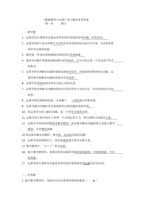
《数据模型与决策》复习题及参考答案第一章绪言一、填空题1.运筹学的主要研究对象是各种有组织系统的管理问题,经营活动。
2.运筹学的核心是运用数学方法研究各种系统的优化途径及方案,为决策者提供科学决策的依据。
3.模型是一件实际事物或现实情况的代表或抽象。
4、通常对问题中变量值的限制称为约束条件,它可以表示成一个等式或不等式的集合。
5.运筹学研究和解决问题的基础是最优化技术,并强调系统整体优化功能。
运筹学研究和解决问题的效果具有连续性。
6.运筹学用系统的观点研究功能之间的关系。
7.运筹学研究和解决问题的优势是应用各学科交叉的方法,具有典型综合应用特性。
8.运筹学的发展趋势是进一步依赖于_计算机的应用和发展。
9.运筹学解决问题时首先要观察待决策问题所处的环境。
10.用运筹学分析与解决问题,是一个科学决策的过程。
11.运筹学的主要目的在于求得一个合理运用人力、物力和财力的最佳方案。
12.运筹学中所使用的模型是数学模型。
用运筹学解决问题的核心是建立数学模型,并对模型求解。
13用运筹学解决问题时,要分析,定议待决策的问题。
14.运筹学的系统特征之一是用系统的观点研究功能关系。
15.数学模型中,“s· t ”表示约束。
16.建立数学模型时,需要回答的问题有性能的客观量度,可控制因素,不可控因素。
17.运筹学的主要研究对象是各种有组织系统的管理问题及经营活动。
二、单选题1. 建立数学模型时,考虑可以由决策者控制的因素是( A )A.销售数量B.销售价格C.顾客的需求D.竞争价格2.我们可以通过(C)来验证模型最优解。
A.观察B.应用C.实验D.调查3.建立运筹学模型的过程不包括( A )阶段。
A.观察环境B.数据分析C.模型设计4. 建立模型的一个基本理由是去揭晓那些重要的或有关的(D.模型实施B)A 数量B变量C约束条件D目标函数5.模型中要求变量取值( D )A可正B可负C非正D非负6. 运筹学研究和解决问题的效果具有(A)A连续性B整体性C阶段性D再生性7.运筹学运用数学方法分析与解决问题,以达到系统的最优目标。
- 1、下载文档前请自行甄别文档内容的完整性,平台不提供额外的编辑、内容补充、找答案等附加服务。
- 2、"仅部分预览"的文档,不可在线预览部分如存在完整性等问题,可反馈申请退款(可完整预览的文档不适用该条件!)。
- 3、如文档侵犯您的权益,请联系客服反馈,我们会尽快为您处理(人工客服工作时间:9:00-18:30)。
CD SUPPLEMENT TO CHAPTER 9
SOME PERSPECTIVES ON SOLVING BINARY INTEGER PROGRAMMING PROBLEMS Review Questions
9s-1 Push the objective function line in the direction of improving values of the objective function. Stop at the last instant when the objective function line passes through a feasible integer point (a binary solution).
9s-2 The exhaustive enumeration method can be used for larger problems while the graphical method is limited to problems with just two variables.
9s-3 The exhaustive enumeration method quickly becomes unwieldy if the number of variable is increased very much.
9s-4 For problems with more than a few variables, it is generally easier to solve linear programming problems than BIP problems of the same size.
9s-5 The LP relaxation of a BIP problem replaces the constraint on each binary variable that the variable is binary by the constraint that it is between 0 and 1.
9s-6 The LP relaxation is relevant for helping to solve a BIP problem because the solution may end up being the solution for the BIP problem, and if not it at least gives a good place to begin the search for an optimal solution.
9s-7 A BIP problem containing mutually exclusive alternative is an example of a problem with special structure.
9s-8 The two primary determinants of computational difficulty for a BIP problem are the number of binary variables and any special structure in the problem.
9s-9 One major pitfall with the rounding procedure is that it may produce a solution that is infeasible for the BIP problem. The other pitfall is that there is no guarantee that a feasible solution will be optimal, or even nearly optimal, for the BIP problem.
Problems
9s-1 a)
b) Optimal solution: (x1, x2) = (0,1).
c) Solving the LP relaxation graphically, the optimal solution is (x1, x2) = (1, 0.667).
This rounds to (1, 1) which is not a feasible solution.
d) Rounding down results in a solution of (1, 0) which is also not a feasible solution. 9s-2 a)
b) Optimal solution: (x1, x2) = (1,1).
c) Solving the LP relaxation graphically, the optimal solution is (x1, x2) = (0, 0.9). This
rounds to (0, 1) which is not a feasible solution.
d) Rounding down results in a solution of (0, 0) which is a feasible solution but yields
Z=0 which in not an optimal solution.
9s-3
9s-4 a) True. The current algorithms for solving BIP problems still are not nearly as efficient as those for solving linear programming problems.
b) True. The two primary determinants of computational difficulty for a BIP problem
are (1) the number of binary variables and (2) any special structure in the problem.
This situation is in contrast to linear programming, where the number of
(functional) constraints is much more important that the number of variables.
c) False. One major pitfall with the rounding procedure is that it may produce a
solution that in infeasible for the BIP problem.。