Flow Simulation New Modules-LAWA
solidworks flow simulation 操作方法

solidworks flow simulation 操作方法【实用版3篇】目录(篇1)一、solidworks flow simulation 操作方法简述1.solidworks flow simulation 简介2.操作方法的主要步骤3.操作方法的优点和局限性二、具体操作步骤1.创建仿真模型2.设定仿真条件3.进行仿真计算4.分析仿真结果5.调整模型参数,重新进行仿真计算三、操作方法的优点和局限性1.优点2.局限性正文(篇1)solidworks flow simulation 是一款广泛应用于流体仿真分析的软件,它的操作方法主要分为以下几个步骤:1.创建仿真模型:首先,我们需要根据实际物理系统,在 solidworks 中建立仿真模型。
这个模型应该尽可能地准确,以便于进行后续的仿真计算。
2.设定仿真条件:接下来,我们需要设定仿真条件,包括流体的物理性质、流速、压力等参数。
这些参数将直接影响仿真的结果。
3.进行仿真计算:在设定好仿真条件后,我们可以开始进行仿真计算。
这个过程需要一定的时间和计算资源,需要耐心等待。
4.分析仿真结果:在仿真计算完成后,我们可以得到仿真结果,包括流体流动的速度、压力、温度等参数。
我们需要对这些参数进行分析,以了解实际物理系统的性能。
5.调整模型参数,重新进行仿真计算:如果分析仿真结果发现模型的参数需要调整,我们可以根据需要进行调整,然后重新进行仿真计算。
solidworks flow simulation 的优点在于它能够快速地进行流体仿真分析,并且能够得到较为准确的结果。
目录(篇2)1.solidworks flow simulation 操作方法介绍2.操作步骤详解3.操作技巧总结正文(篇2)一、solidworks flow simulation 操作方法介绍solidworks flow simulation 是一款专业的流体模拟软件,可应用于机械设计、汽车设计、航空航天等领域。
solidworks_flow_simulation中文教程
目录第一阶段:球阀设计打开模型……………………………………………………………………………1-1创建b 项目…………………………………………………………………1-2边界条件……………………………………………………………………………1-5定义工程目标…………………………………………………………………………1-7求解……………………………………………………………………………………1- 8监测求解过程…………………………………………………………………………1-8调整模型透明度………………………………………………………………………1-10切面云图……………………………………………………………………………1-10表面云图………………………………………………………………………………1-11等值图………………………………………………………………………………1-12流动迹线图…………………………………………………………………………1-13 XY 图………………………………………………………………………………1-15表面参数………………………………………………………………………………1-16分析球形部分中一个设计变化……………………………………………………… 1-16复制项目……………………………………………………………………………1-19分析b 应用中的一个设计变化……………………………………………1-19第一阶段:耦合热交换打开模型………………………………………………………………………………2-1 准备模型……………………………………………………………………………2-2 创建b 项目………………………………………………………………… 2-3 定义风扇………………………………………………………………………………2-6 定义边界条件…………………………………………………………………………2-8 定义热源………………………………………………………………………………2-9 创建新材料…………………………………………………………………………2-10 定义固体材料…………………………………………………………………………2-10 定义工程目标…………………………………………………………………………2-11 定义体积目标…………………………………………………………………… 2-11 定义表面目标…………………………………………………………………… 2-13定义全局目标…………………………………………………………………… 2-14改变几何求解精度…………………………………………………………………2-15 求解…………………………………………………………………………………2-16 观察目标………………………………………………………………………………2-16 流动迹线图…………………………………………………………………………2-17 切面云图……………………………………………………………………………2-19 表面云图……………………………………………………………………………2-22第一阶段:多孔介质打开模型………………………………………………………………………………3-2 创建b 项目…………………………………………………………………3-2 定义边界条件…………………………………………………………………………3-4 创建一个等向性的多孔介质………………………………………………………3-5 定义多孔介质-等向性………………………………………………………3-7 定义表面目标………………………………………………………………………… 3-7 定义方程目标………………………………………………………………………3-8 求解……………………………………………………………………………………3-9 观察目标……………………………………………………………………………… 3-10 流动迹线图…………………………………………………………………………… 3-10 复制项目……………………………………………………………………………… 3-11 创建一个单向性的多孔介质………………………………………………………… 3-12 定义多孔介质-单向性……………………………………………………………… 3-12 比较等向性和单向性多孔介质……………………………………………………… 3-13确定水力损失模型描述……………………………………………………………………………4-2 创建项目……………………………………………………………………………… 4-3 定义边界条件………………………………………………………………………… 4-7 定义表面目标………………………………………………………………………… 4-8 运行计算……………………………………………………………………………… 4-9 监测计算……………………………………………………………………………… 4-10 复制项目……………………………………………………………………………… 4-10 创建切面云图………………………………………………………………………… 4-11创建全局目标………………………………………………………………………… 4-15 计算器使用…………………………………………………………………………… 4-16 改变几何参数………………………………………………………………………… 4-18圆柱体阻力系数创建项目…………………………………………………………………………… 5-2 定义2D 流动平面………………………………………………………………… 5-6 定义全局目标……………………………………………………………………… 5-7 定义方程目标……………………………………………………………………… 5-7 复制项目并且创建一个新例子…………………………………………………… 5-8 改变项目设置………………………………………………………………………5-9 改变方程目标………………………………………………………………………5-10 创建模板…………………………………………………………………………… 5-10 以模板方式创建一个项目………………………………………………………… 5-11 求解一系列项目…………………………………………………………………… 5-12 获取结果…………………………………………………………………………… 5-12 热交换系数打开模型…………………………………………………………………………… 6-2 创建项目…………………………………………………………………………… 6-3 对称边界条件……………………………………………………………………… 6-5 定义流体子区域…………………………………………………………………… 6-6 定义边界条件……………………………………………………………………… 6-7 定义固体材料……………………………………………………………………… 6-10 定义体积目标……………………………………………………………………… 6-11 运行求解…………………………………………………………………………… 6-11 观察目标…………………………………………………………………………… 6-12显示流动迹线图…………………………………………………………………… 6-14 计算表面参数……………………………………………………………………… 6-16 计算热交换系数…………………………………………………………………… 6-18 定义参数显示范围…………………………………………………………………6-18网格优化问题描述…………………………………………………………………………… 7-2 模型定义…………………………………………………………………………… 7-3 定义项目……………………………………………………………………………7-3 边界条件……………………………………………………………………………7-3 手动设置最小网格间隙尺寸……………………………………………………… 7-7 关闭自动网格定义…………………………………………………………………7-9 生成网格如下所示,约75000网格单元使用Local Intial Mesh 选项…………………………………………………7-10 定义控制平面………………………………………………………………………7-12 再创建一个局部初始网格…………………………………………………………7-14EFD Zooming的应用问题描述……………………………………………………………………………8-1 两种使用b 进行求解问题的方式…………………………………………8-3 EFD Zooming 方法步骤……………………………………………………………8-3 EFD Zooming 第一阶段………………………………………………………8-4 EFD Zooming 项目第一阶段…………………………………………………8-4 EFD Zooming 第二阶段………………………………………………………8-8 EFD Zooming 项目第二阶段…………………………………………………8-8 改变散热器……………………………………………………………………8-14 复制项目到存在的模型定义…………………………………………………8-14局部初始化网格方法………………………………………………………………8-15 使用局部初始化网格方法的b 项目(Sink No1) …………………… 8-15 使用局部初始化网格方法的b 项目(Sink No2) …………………… 8-18 结果………………………………………………………………………………… 8-18纺织机械问题描述…………………………………………………………………………… 9-1 模型定义…………………………………………………………………………… 9-2 定义项目…………………………………………………………………………… 9-3 边界条件…………………………………………………………………………… 9-3 定义旋转壁面……………………………………………………………………… 9-4 初始条件-旋转…………………………………………………………………… 9-5 定义目标…………………………………………………………………………… 9-6 结果-光滑表面…………………………………………………………………… 9-7 显示粒子流和流动迹线……………………………………………………………9-8 模拟粗糙旋转壁面………………………………………………………………… 9-10 改变壁面粗糙度…………………………………………………………………… 9-10 结果-粗糙壁面…………………………………………………………………… 9-11圆形通道中的非牛顿流体流动问题描述………………………………………………………………………………10-1 模型定义………………………………………………………………………………10-2 定义非牛顿流体……………………………………………………………………… 10-2 定义项目………………………………………………………………………………10-2 边界条件………………………………………………………………………………10-3 定义目标…………………………………………………………………………10-3 与流体水进行比较…………………………………………………………………… 10-4 改变项目设置……………………………………………………………………10-4具有反射镜和屏幕的加热球问题描述…………………………………………………………………………… 11-1 模型结构…………………………………………………………………………… 11-2 案例 1 ………………………………………………………………………………11-3 定义项目……………………………………………………………………… 11-3 定义计算域……………………………………………………………………11-3 调整自动网格设置……………………………………………………………11-4 定义辐射表面…………………………………………………………………11-4 定义物体对于热辐射的可穿透性…………………………………………… 11-5 热源和目标定义………………………………………………………………11-5 案例 2 ……………………………………………………………………………… 11-6 改变辐射表面状况……………………………………………………………11-6 定义全局目标…………………………………………………………………11-6 定义固体的初始条件…………………………………………………………11-6结果………………………………………………………………………………… 11-7旋转叶轮问题描述………………………………………………………………………………12-1 模型定义………………………………………………………………………………12-2 定义项目………………………………………………………………………………12-2 边界条件………………………………………………………………………………12-3 定义静止壁面……………………………………………………………………12-4 叶轮效率………………………………………………………………………………12-4 定义项目目标…………………………………………………………………………12-5 结果……………………………………………………………………………………12-7CPU 冷却器问题描述………………………………………………………………………………13-1 模型定义………………………………………………………………………………13-2 定义项目………………………………………………………………………………13-2 定义计算域……………………………………………………………………………13-2 旋转区域………………………………………………………………………………13-3 定义静止壁面…………………………………………………………………………13-5 固体材料………………………………………………………………………………13-6 热源……………………………………………………………………………………13-6 初始网格设置…………………………………………………………………………13-7结果……………………………………………………………………………………13-11特性列表下面罗列了出现在教程中的b 相应的物理和界面特性。
solidworks flow simulation 要点 -回复

solidworks flow simulation 要点-回复【Solidworks Flow Simulation 要点】Solidworks Flow Simulation是一款流体力学模拟软件,它可以帮助工程师对流体流动行为进行仿真和分析。
本文将深入探讨Solidworks Flow Simulation的要点,并逐步回答以下问题:它是如何工作的?有哪些应用领域?如何设置流体材料和边界条件?如何进行仿真和分析?以及如何优化设计。
一、Solidworks Flow Simulation是如何工作的?Solidworks Flow Simulation基于有限元和有限体积方法,通过对流场的连续方程进行离散求解,并结合各个特定条件和边界条件,模拟出流体的流动行为。
它采用了计算流体动力学(CFD)技术,可以模拟各种复杂的工程问题,如流体流动、热传导、质量传输等。
二、Solidworks Flow Simulation的应用领域有哪些?Solidworks Flow Simulation广泛应用于多个行业,包括机械、汽车、航空航天、能源等。
其应用领域涵盖了气体和液体的流动模拟,如风扇、泵、管道、喷嘴、飞机机翼等。
此外,它还可以用于热管理和热传导分析,比如散热器、冷却系统等。
三、如何设置流体材料和边界条件?在使用Solidworks Flow Simulation之前,我们需要设置流体的物理特性和边界条件。
首先,我们需要选择合适的流体模型,例如理想气体、液体等,并设置其初始和边界条件。
然后,我们可以定义流体的速度、压力、温度等参数,并设置边界条件,如入口和出口条件、壁面条件等。
四、如何进行仿真和分析?在设置完流体材料和边界条件后,我们可以开始进行仿真和分析。
首先,我们需要创建一个流体域并进行网格划分,以获得更准确的仿真结果。
然后,我们可以选择合适的求解器并设置计算精度。
接下来,我们可以进行初始条件的求解和迭代计算,直到收敛为止。
SOLIDWORKS Flow Simulation 用户手册说明书
SOLIDWORKS SOLIDWORKS Flow SimulationDassault Systèmes SolidWorks Corporation175 Wyman StreetWaltham, MA 02451 U.S.A.© 1995-2021, Dassault Systemes SolidWorks Corporation, a Dassault Systèmes SE company, 175 Wyman Street, Waltham, Mass. 02451 USA. All Rights Reserved.The information and the software discussed in this document are subject to change without notice and are not commitments by Dassault Systemes SolidWorks Corporation (DS SolidWorks).No material may be reproduced or transmitted in any form or by any means, electronically or manually, for any purpose without the express written permission of DS SolidWorks.The software discussed in this document is furnished under a license and may be used or copied only in accordance with the terms of the license. All warranties given by DS SolidWorks as to the software and documentation are set forth in the license agreement, and nothing stated in, or implied by, this document or its contents shall be considered or deemed a modification or amendment of any terms, including warranties, in the license agreement.For a full list of the patents, trademarks, and third-party software contained in this release, please go to the Legal Notices in the SOLIDWORKS documentation.Restricted RightsThis clause applies to all acquisitions of Dassault Systèmes Offerings by or for the United States federal government, or by any prime contractor or subcontractor (at any tier) under any contract, grant, cooperative agreement or other activity with the federal government. The software, documentation and any other technical data provided hereunder is commercial in nature and developed solely at private expense. The Software is delivered as "Commercial Computer Software" as defined in DFARS 252.227-7014 (June 1995) or as a "Commercial Item" as defined in FAR 2.101(a) and as such is provided with only such rights as are provided in Dassault Systèmes standard commercial end user license agreement. Technical data is provided with limited rights only as provided in DFAR 252.227-7015 (Nov. 1995) or FAR 52.227-14 (June 1987), whichever is applicable. The terms and conditions of the Dassault Systèmes standard commercial end user license agreement shall pertain to the United States government's use and disclosure of this software, and shall supersede any conflicting contractual terms and conditions. If the DS standard commercial license fails to meet the United States government's needs or is inconsistent in any respect with United States Federal law, the United States government agrees to return this software, unused, to DS. The following additional statement applies only to acquisitions governed by DFARS Subpart 227.4 (October 1988): "Restricted Rights - use, duplication and disclosure by the Government is subject to restrictions as set forth in subparagraph (c)(l)(ii) of the Rights in Technical Data and Computer Software clause at DFARS 252-227-7013 (Oct. 1988)."In the event that you receive a request from any agency of the U.S. Government to provide Software with rights beyond those set forth above, you will notify DS SolidWorks of the scope of the request and DS SolidWorks will have five (5) business days to, in its sole discretion, accept or reject such request. Contractor/ Manufacturer: Dassault Systemes SolidWorks Corporation, 175 Wyman Street, Waltham, Massachusetts 02451 USA.Document Number: PMT2243-ENGContents IntroductionAbout This Course . . . . . . . . . . . . . . . . . . . . . . . . . . . . . . . . . . . . . . . . 2Prerequisites . . . . . . . . . . . . . . . . . . . . . . . . . . . . . . . . . . . . . . . . . . 2Course Design Philosophy . . . . . . . . . . . . . . . . . . . . . . . . . . . . . . . 2Using this Book . . . . . . . . . . . . . . . . . . . . . . . . . . . . . . . . . . . . . . . 2Lessons . . . . . . . . . . . . . . . . . . . . . . . . . . . . . . . . . . . . . . . . . . . . . . 2About the Training Files. . . . . . . . . . . . . . . . . . . . . . . . . . . . . . . . . 3Windows. . . . . . . . . . . . . . . . . . . . . . . . . . . . . . . . . . . . . . . . . . . . . 3User Interface Appearance . . . . . . . . . . . . . . . . . . . . . . . . . . . . . . . 3Conventions Used in this Book . . . . . . . . . . . . . . . . . . . . . . . . . . . 3Use of Color . . . . . . . . . . . . . . . . . . . . . . . . . . . . . . . . . . . . . . . . . . 4More SOLIDWORKS Training Resources. . . . . . . . . . . . . . . . . . . . . . 4Local User Groups . . . . . . . . . . . . . . . . . . . . . . . . . . . . . . . . . . . . . 4 Lesson 1:Creating a SOLIDWORKS Flow Simulation ProjectObjectives. . . . . . . . . . . . . . . . . . . . . . . . . . . . . . . . . . . . . . . . . . . . . . . 5Case Study: Manifold Assembly. . . . . . . . . . . . . . . . . . . . . . . . . . . . . . 6Problem Description. . . . . . . . . . . . . . . . . . . . . . . . . . . . . . . . . . . . . . . 6Stages in the Process. . . . . . . . . . . . . . . . . . . . . . . . . . . . . . . . . . . . 6Model Preparation. . . . . . . . . . . . . . . . . . . . . . . . . . . . . . . . . . . . . . . . . 7Internal Flow Analysis . . . . . . . . . . . . . . . . . . . . . . . . . . . . . . . . . . 7External Flow Analysis. . . . . . . . . . . . . . . . . . . . . . . . . . . . . . . . . . 7Manifold Analysis. . . . . . . . . . . . . . . . . . . . . . . . . . . . . . . . . . . . . . 8Lids. . . . . . . . . . . . . . . . . . . . . . . . . . . . . . . . . . . . . . . . . . . . . . . . . 8Lid Thickness . . . . . . . . . . . . . . . . . . . . . . . . . . . . . . . . . . . . . . . . . 9Manual Lid Creation. . . . . . . . . . . . . . . . . . . . . . . . . . . . . . . . . . . . 9iContents SOLIDWORKS SimulationiiAdding a Lid to a Part File . . . . . . . . . . . . . . . . . . . . . . . . . . . . . . . 9 Adding a Lid to an Assembly File . . . . . . . . . . . . . . . . . . . . . . . . 10 Checking the Geometry . . . . . . . . . . . . . . . . . . . . . . . . . . . . . . . . 12 Internal Fluid Volume. . . . . . . . . . . . . . . . . . . . . . . . . . . . . . . . . . 13 Invalid Contacts . . . . . . . . . . . . . . . . . . . . . . . . . . . . . . . . . . . . . . 13 Project Wizard . . . . . . . . . . . . . . . . . . . . . . . . . . . . . . . . . . . . . . . 18 Dependency . . . . . . . . . . . . . . . . . . . . . . . . . . . . . . . . . . . . . . . . . 21 Exclude Cavities Without Flow Conditions. . . . . . . . . . . . . . . . . 21 Adiabatic Wall . . . . . . . . . . . . . . . . . . . . . . . . . . . . . . . . . . . . . . . 22 Roughness. . . . . . . . . . . . . . . . . . . . . . . . . . . . . . . . . . . . . . . . . . . 22 Computational Domain. . . . . . . . . . . . . . . . . . . . . . . . . . . . . . . . . 24 Mesh . . . . . . . . . . . . . . . . . . . . . . . . . . . . . . . . . . . . . . . . . . . . . . . 31 Load Results Option. . . . . . . . . . . . . . . . . . . . . . . . . . . . . . . . . . . 31 Monitoring the Solver. . . . . . . . . . . . . . . . . . . . . . . . . . . . . . . . . . 32 Goal Plot Window . . . . . . . . . . . . . . . . . . . . . . . . . . . . . . . . . . . . 33 Warning Messages . . . . . . . . . . . . . . . . . . . . . . . . . . . . . . . . . . . . 33 Post-processing. . . . . . . . . . . . . . . . . . . . . . . . . . . . . . . . . . . . . . . . . . 36 Scaling the Limits of the Legend . . . . . . . . . . . . . . . . . . . . . . . . . 38 Changing Legend Settings . . . . . . . . . . . . . . . . . . . . . . . . . . . . . . 38 Orientation of the Legend, Logarithmic Scale . . . . . . . . . . . . . . . 38 Discussion. . . . . . . . . . . . . . . . . . . . . . . . . . . . . . . . . . . . . . . . . . . . . . 51 Summary. . . . . . . . . . . . . . . . . . . . . . . . . . . . . . . . . . . . . . . . . . . . . . . 51 Exercise 1: Air Conditioning Ducting . . . . . . . . . . . . . . . . . . . . . . . . 52Lesson 2:MeshingObjectives. . . . . . . . . . . . . . . . . . . . . . . . . . . . . . . . . . . . . . . . . . . . . . 59Case Study: Chemistry Hood . . . . . . . . . . . . . . . . . . . . . . . . . . . . . . . 60Project Description. . . . . . . . . . . . . . . . . . . . . . . . . . . . . . . . . . . . . . . 60Computational Mesh. . . . . . . . . . . . . . . . . . . . . . . . . . . . . . . . . . . . . . 64Basic Mesh . . . . . . . . . . . . . . . . . . . . . . . . . . . . . . . . . . . . . . . . . . . . . 64Initial Mesh. . . . . . . . . . . . . . . . . . . . . . . . . . . . . . . . . . . . . . . . . . . . . 64Geometry Resolution . . . . . . . . . . . . . . . . . . . . . . . . . . . . . . . . . . . . . 65Minimum Gap Size. . . . . . . . . . . . . . . . . . . . . . . . . . . . . . . . . . . . 65Minimum Wall Thickness . . . . . . . . . . . . . . . . . . . . . . . . . . . . . . 65Result Resolution/Level of Initial Mesh. . . . . . . . . . . . . . . . . . . . . . . 68Manual Global Mesh Settings. . . . . . . . . . . . . . . . . . . . . . . . . . . . 70Control Planes. . . . . . . . . . . . . . . . . . . . . . . . . . . . . . . . . . . . . . . . . . . 73Summary. . . . . . . . . . . . . . . . . . . . . . . . . . . . . . . . . . . . . . . . . . . . . . . 83Exercise 2: Square Ducting. . . . . . . . . . . . . . . . . . . . . . . . . . . . . . . . . 84Exercise 3: Thin Walled Box . . . . . . . . . . . . . . . . . . . . . . . . . . . . . . . 91Exercise 4: Heat Sink . . . . . . . . . . . . . . . . . . . . . . . . . . . . . . . . . . . . . 97Exercise 5: Meshing Valve Assembly . . . . . . . . . . . . . . . . . . . . . . . 102Boundary Conditions . . . . . . . . . . . . . . . . . . . . . . . . . . . . . . . . . 102SOLIDWORKS Simulation Contents Lesson 3:Thermal AnalysisObjectives. . . . . . . . . . . . . . . . . . . . . . . . . . . . . . . . . . . . . . . . . . . . . 103Case Study: Electronics Enclosure. . . . . . . . . . . . . . . . . . . . . . . . . . 104Project Description. . . . . . . . . . . . . . . . . . . . . . . . . . . . . . . . . . . . . . 104Fans. . . . . . . . . . . . . . . . . . . . . . . . . . . . . . . . . . . . . . . . . . . . . . . . . . 111Fan Curves . . . . . . . . . . . . . . . . . . . . . . . . . . . . . . . . . . . . . . . . . 111Derating . . . . . . . . . . . . . . . . . . . . . . . . . . . . . . . . . . . . . . . . . . . 111Perforated Plates. . . . . . . . . . . . . . . . . . . . . . . . . . . . . . . . . . . . . . . . 113Free Area Ratio. . . . . . . . . . . . . . . . . . . . . . . . . . . . . . . . . . . . . . 115Discussion. . . . . . . . . . . . . . . . . . . . . . . . . . . . . . . . . . . . . . . . . . . . . 119Summary. . . . . . . . . . . . . . . . . . . . . . . . . . . . . . . . . . . . . . . . . . . . . . 119Exercise 6: Materials with Orthotropic Thermal Conductivity . . . . 120Exercise 7: Electric Wire . . . . . . . . . . . . . . . . . . . . . . . . . . . . . . . . . 126Summary. . . . . . . . . . . . . . . . . . . . . . . . . . . . . . . . . . . . . . . . . . . . . . 132 Lesson 4:External Transient AnalysisObjectives. . . . . . . . . . . . . . . . . . . . . . . . . . . . . . . . . . . . . . . . . . . . . 133Case Study: Flow Around a Cylinder. . . . . . . . . . . . . . . . . . . . . . . . 134Problem Description. . . . . . . . . . . . . . . . . . . . . . . . . . . . . . . . . . . . . 134Stages in the Process. . . . . . . . . . . . . . . . . . . . . . . . . . . . . . . . . . 135Reynolds Number. . . . . . . . . . . . . . . . . . . . . . . . . . . . . . . . . . . . . . . 135External Flow . . . . . . . . . . . . . . . . . . . . . . . . . . . . . . . . . . . . . . . . . . 135Transient Analysis. . . . . . . . . . . . . . . . . . . . . . . . . . . . . . . . . . . . . . . 137Turbulence Intensity. . . . . . . . . . . . . . . . . . . . . . . . . . . . . . . . . . . . . 137Solution Adaptive Mesh Refinement . . . . . . . . . . . . . . . . . . . . . . . . 138Two Dimensional Flow. . . . . . . . . . . . . . . . . . . . . . . . . . . . . . . . . . . 138Computational Domain. . . . . . . . . . . . . . . . . . . . . . . . . . . . . . . . . . . 139Calculation Control Options. . . . . . . . . . . . . . . . . . . . . . . . . . . . . . . 139Finishing. . . . . . . . . . . . . . . . . . . . . . . . . . . . . . . . . . . . . . . . . . . 140Refinement . . . . . . . . . . . . . . . . . . . . . . . . . . . . . . . . . . . . . . . . . 140Solving . . . . . . . . . . . . . . . . . . . . . . . . . . . . . . . . . . . . . . . . . . . . 140Saving. . . . . . . . . . . . . . . . . . . . . . . . . . . . . . . . . . . . . . . . . . . . . 140Drag Equation. . . . . . . . . . . . . . . . . . . . . . . . . . . . . . . . . . . . . . . 142Unsteady Vortex Shedding. . . . . . . . . . . . . . . . . . . . . . . . . . . . . 144Time Animation . . . . . . . . . . . . . . . . . . . . . . . . . . . . . . . . . . . . . . . . 145Discussion. . . . . . . . . . . . . . . . . . . . . . . . . . . . . . . . . . . . . . . . . . . . . 149Summary. . . . . . . . . . . . . . . . . . . . . . . . . . . . . . . . . . . . . . . . . . . . . . 149Exercise 8: Electronics Cooling . . . . . . . . . . . . . . . . . . . . . . . . . . . . 150iiiContents SOLIDWORKS Simulation Lesson 5:Conjugate Heat TransferObjectives. . . . . . . . . . . . . . . . . . . . . . . . . . . . . . . . . . . . . . . . . . . . . 161Case Study: Heated Cold Plate. . . . . . . . . . . . . . . . . . . . . . . . . . . . . 162Project Description. . . . . . . . . . . . . . . . . . . . . . . . . . . . . . . . . . . . . . 162Stages in the Process. . . . . . . . . . . . . . . . . . . . . . . . . . . . . . . . . . 162Conjugate Heat Transfer. . . . . . . . . . . . . . . . . . . . . . . . . . . . . . . . . . 163Real Gases. . . . . . . . . . . . . . . . . . . . . . . . . . . . . . . . . . . . . . . . . . . . . 163Goals Plot in the Solver Window. . . . . . . . . . . . . . . . . . . . . . . . 166Summary. . . . . . . . . . . . . . . . . . . . . . . . . . . . . . . . . . . . . . . . . . . . . . 168Exercise 9: Heat Exchanger with Multiple Fluids . . . . . . . . . . . . . . 169 Lesson 6:EFD ZoomingObjectives. . . . . . . . . . . . . . . . . . . . . . . . . . . . . . . . . . . . . . . . . . . . . 173Case Study: Electronics Enclosure. . . . . . . . . . . . . . . . . . . . . . . . . . 174Project Description. . . . . . . . . . . . . . . . . . . . . . . . . . . . . . . . . . . . . . 174EFD Zooming. . . . . . . . . . . . . . . . . . . . . . . . . . . . . . . . . . . . . . . . . . 174EFD Zooming - Computational Domain . . . . . . . . . . . . . . . . . . 177Summary. . . . . . . . . . . . . . . . . . . . . . . . . . . . . . . . . . . . . . . . . . . . . . 184 Lesson 7:Porous MediaObjectives. . . . . . . . . . . . . . . . . . . . . . . . . . . . . . . . . . . . . . . . . . . . . 185Case Study: Catalytic Converter. . . . . . . . . . . . . . . . . . . . . . . . . . . . 186Problem Description. . . . . . . . . . . . . . . . . . . . . . . . . . . . . . . . . . . . . 186Stages in the Process. . . . . . . . . . . . . . . . . . . . . . . . . . . . . . . . . . 186Associated Goal . . . . . . . . . . . . . . . . . . . . . . . . . . . . . . . . . . . . . 187Porous Media . . . . . . . . . . . . . . . . . . . . . . . . . . . . . . . . . . . . . . . . . . 189Porosity. . . . . . . . . . . . . . . . . . . . . . . . . . . . . . . . . . . . . . . . . . . . 189Permeability Type. . . . . . . . . . . . . . . . . . . . . . . . . . . . . . . . . . . . 189Resistance. . . . . . . . . . . . . . . . . . . . . . . . . . . . . . . . . . . . . . . . . . 189Matrix and Fluid Heat Exchange . . . . . . . . . . . . . . . . . . . . . . . . 189Specific area . . . . . . . . . . . . . . . . . . . . . . . . . . . . . . . . . . . . . . . . 189Dummy Bodies. . . . . . . . . . . . . . . . . . . . . . . . . . . . . . . . . . . . . . 192Design Modification. . . . . . . . . . . . . . . . . . . . . . . . . . . . . . . . . . . . . 197Discussion. . . . . . . . . . . . . . . . . . . . . . . . . . . . . . . . . . . . . . . . . . . . . 201Summary. . . . . . . . . . . . . . . . . . . . . . . . . . . . . . . . . . . . . . . . . . . . . . 201Exercise 10: Channel Flow. . . . . . . . . . . . . . . . . . . . . . . . . . . . . . . . 202 Lesson 8:Rotating Reference FramesObjectives. . . . . . . . . . . . . . . . . . . . . . . . . . . . . . . . . . . . . . . . . . . . . 209Rotating Reference Frame . . . . . . . . . . . . . . . . . . . . . . . . . . . . . . . . 210Part 1: Averaging. . . . . . . . . . . . . . . . . . . . . . . . . . . . . . . . . . . . . . . . 210Case Study: Table Fan . . . . . . . . . . . . . . . . . . . . . . . . . . . . . . . . . . . 210Problem Description. . . . . . . . . . . . . . . . . . . . . . . . . . . . . . . . . . . . . 211Stages in the Process. . . . . . . . . . . . . . . . . . . . . . . . . . . . . . . . . . 211 ivSOLIDWORKS Simulation ContentsNoise Prediction . . . . . . . . . . . . . . . . . . . . . . . . . . . . . . . . . . . . . . . . 217Broadband Model. . . . . . . . . . . . . . . . . . . . . . . . . . . . . . . . . . . . 217Part 2: Sliding Mesh. . . . . . . . . . . . . . . . . . . . . . . . . . . . . . . . . . . . . 218Case Study: Blower Fan. . . . . . . . . . . . . . . . . . . . . . . . . . . . . . . . . . 218Problem Description. . . . . . . . . . . . . . . . . . . . . . . . . . . . . . . . . . . . . 218Tangential Faces of Rotors . . . . . . . . . . . . . . . . . . . . . . . . . . . . . . . . 220Time Step . . . . . . . . . . . . . . . . . . . . . . . . . . . . . . . . . . . . . . . . . . . . . 223Part 3: Axial Periodicity . . . . . . . . . . . . . . . . . . . . . . . . . . . . . . . . . . 225Summary. . . . . . . . . . . . . . . . . . . . . . . . . . . . . . . . . . . . . . . . . . . . . . 228Exercise 11: Ceiling Fan. . . . . . . . . . . . . . . . . . . . . . . . . . . . . . . . . . 229Boundary Conditions . . . . . . . . . . . . . . . . . . . . . . . . . . . . . . . . . 229Computational Domain. . . . . . . . . . . . . . . . . . . . . . . . . . . . . . . . 230 Lesson 9:Parametric StudyObjectives. . . . . . . . . . . . . . . . . . . . . . . . . . . . . . . . . . . . . . . . . . . . . 231Case Study: Piston Valve . . . . . . . . . . . . . . . . . . . . . . . . . . . . . . . . . 232Problem Description. . . . . . . . . . . . . . . . . . . . . . . . . . . . . . . . . . . . . 232Stages in the Process. . . . . . . . . . . . . . . . . . . . . . . . . . . . . . . . . . 232Parametric Analysis . . . . . . . . . . . . . . . . . . . . . . . . . . . . . . . . . . . . . 233Steady State Analysis . . . . . . . . . . . . . . . . . . . . . . . . . . . . . . . . . . . . 233Parametric Study. . . . . . . . . . . . . . . . . . . . . . . . . . . . . . . . . . . . . 235Part 1: Goal Optimization. . . . . . . . . . . . . . . . . . . . . . . . . . . . . . . . . 236Input Variable Types . . . . . . . . . . . . . . . . . . . . . . . . . . . . . . . . . 237Target Value Dependence Types . . . . . . . . . . . . . . . . . . . . . . . . 238Output Variable Initial Values . . . . . . . . . . . . . . . . . . . . . . . . . . 239Running Optimization Study . . . . . . . . . . . . . . . . . . . . . . . . . . . 239Part 2: Design Scenario. . . . . . . . . . . . . . . . . . . . . . . . . . . . . . . . . . . 243Part 3: Multi parameter Optimization. . . . . . . . . . . . . . . . . . . . . . . . 246Summary. . . . . . . . . . . . . . . . . . . . . . . . . . . . . . . . . . . . . . . . . . . . . . 250Exercise 12: Variable Geometry Dependent Solution . . . . . . . . . . . 251Boundary Conditions . . . . . . . . . . . . . . . . . . . . . . . . . . . . . . . . . 252 Lesson 10:Free SurfaceObjectives. . . . . . . . . . . . . . . . . . . . . . . . . . . . . . . . . . . . . . . . . . . . . 253Case Study: Water Tank . . . . . . . . . . . . . . . . . . . . . . . . . . . . . . . . . . 254Problem Description. . . . . . . . . . . . . . . . . . . . . . . . . . . . . . . . . . . . . 254Free Surface . . . . . . . . . . . . . . . . . . . . . . . . . . . . . . . . . . . . . . . . . . . 254Volume of Fluid (VOF) . . . . . . . . . . . . . . . . . . . . . . . . . . . . . . . 254Summary. . . . . . . . . . . . . . . . . . . . . . . . . . . . . . . . . . . . . . . . . . . . . . 261Exercise 13: Water Jet . . . . . . . . . . . . . . . . . . . . . . . . . . . . . . . . . . . 262Theoretical Results. . . . . . . . . . . . . . . . . . . . . . . . . . . . . . . . . . . . . . 268Summary. . . . . . . . . . . . . . . . . . . . . . . . . . . . . . . . . . . . . . . . . . . . . . 268Exercise 14: Dam-Break Flow . . . . . . . . . . . . . . . . . . . . . . . . . . . . . 269Experimental Data . . . . . . . . . . . . . . . . . . . . . . . . . . . . . . . . . . . . . . 275Summary. . . . . . . . . . . . . . . . . . . . . . . . . . . . . . . . . . . . . . . . . . . . . . 276References. . . . . . . . . . . . . . . . . . . . . . . . . . . . . . . . . . . . . . . . . . . . . 276vContents SOLIDWORKS Simulation Lesson 11:CavitationObjectives. . . . . . . . . . . . . . . . . . . . . . . . . . . . . . . . . . . . . . . . . . . . . 277Case Study: Cone Valve . . . . . . . . . . . . . . . . . . . . . . . . . . . . . . . . . . 278Problem Description. . . . . . . . . . . . . . . . . . . . . . . . . . . . . . . . . . . . . 278Cavitation . . . . . . . . . . . . . . . . . . . . . . . . . . . . . . . . . . . . . . . . . . . . . 278Discussion. . . . . . . . . . . . . . . . . . . . . . . . . . . . . . . . . . . . . . . . . . . . . 281Summary. . . . . . . . . . . . . . . . . . . . . . . . . . . . . . . . . . . . . . . . . . . . . . 281 Lesson 12:Relative HumidityObjectives. . . . . . . . . . . . . . . . . . . . . . . . . . . . . . . . . . . . . . . . . . . . . 283Relative Humidity. . . . . . . . . . . . . . . . . . . . . . . . . . . . . . . . . . . . . . . 284Case Study: Cook House . . . . . . . . . . . . . . . . . . . . . . . . . . . . . . . . . 284Problem Description. . . . . . . . . . . . . . . . . . . . . . . . . . . . . . . . . . . . . 284Summary. . . . . . . . . . . . . . . . . . . . . . . . . . . . . . . . . . . . . . . . . . . . . . 290 Lesson 13:Particle TrajectoryObjectives. . . . . . . . . . . . . . . . . . . . . . . . . . . . . . . . . . . . . . . . . . . . . 291Case Study: Hurricane Generator. . . . . . . . . . . . . . . . . . . . . . . . . . . 292Problem Description. . . . . . . . . . . . . . . . . . . . . . . . . . . . . . . . . . . . . 292Particle Trajectories - Overview. . . . . . . . . . . . . . . . . . . . . . . . . . . . 292Particle Study - Physical Settings. . . . . . . . . . . . . . . . . . . . . . . . 297Particle Study - Wall Condition . . . . . . . . . . . . . . . . . . . . . . . . . 298Summary. . . . . . . . . . . . . . . . . . . . . . . . . . . . . . . . . . . . . . . . . . . . . . 299Exercise 15: Uniform Flow Stream. . . . . . . . . . . . . . . . . . . . . . . . . 300 Lesson 14:Supersonic FlowObjectives. . . . . . . . . . . . . . . . . . . . . . . . . . . . . . . . . . . . . . . . . . . . . 305Supersonic Flow. . . . . . . . . . . . . . . . . . . . . . . . . . . . . . . . . . . . . . . . 306Case Study: Conical Body . . . . . . . . . . . . . . . . . . . . . . . . . . . . . . . . 306Problem Description. . . . . . . . . . . . . . . . . . . . . . . . . . . . . . . . . . . . . 306Drag Coefficient. . . . . . . . . . . . . . . . . . . . . . . . . . . . . . . . . . . . . 307Shock Waves. . . . . . . . . . . . . . . . . . . . . . . . . . . . . . . . . . . . . . . . 311Discussion. . . . . . . . . . . . . . . . . . . . . . . . . . . . . . . . . . . . . . . . . . . . . 312Summary. . . . . . . . . . . . . . . . . . . . . . . . . . . . . . . . . . . . . . . . . . . . . . 312 Lesson 15:FEA Load TransferObjectives. . . . . . . . . . . . . . . . . . . . . . . . . . . . . . . . . . . . . . . . . . . . . 313Case Study: Billboard. . . . . . . . . . . . . . . . . . . . . . . . . . . . . . . . . . . . 314Problem Description. . . . . . . . . . . . . . . . . . . . . . . . . . . . . . . . . . . . . 314Summary. . . . . . . . . . . . . . . . . . . . . . . . . . . . . . . . . . . . . . . . . . . . . . 318 vi。
Solidworksflowsimulation实例分析演示幻灯片

8、二维流动
定义流动对称条件和域的大小
? 在SolidWorks flow simulation tree中,右击input data下的 computational domain,选择edit definition
式中,??为流体的密度,v为自由流的速度(平均
速度),A为前沿面积,Cd为阻力系数。
2020/4/13
19
? 插入方程式目标---右键单击goal选择insert equation goal,在expression中输入公式:{GG 力 (X) 1}*2*998.19/1.01241e-3^2*0.01/0.001/140^2 , 在dimensionality(量纲)中选择no unit(无 单位)
Solidworks flow simulation 外流瞬态分析示例
2
1
1、实例分析:圆柱绕流
? 使用二维平面流动分析围绕一个圆柱体的流 体流动
? 温度和压力分别为293.1K和 1atm(1atm=101325Pa)的水流过直径为0.01m, 高为0.01m的圆柱体,流动的雷诺数为140, 计算其对应的阻力系数,湍流强度为1%。
Result &geometry resolution(结 设置 geometry resolution为7 果及几何精细度)
2020/4/13
6
2020/4/13
7
2020/4/13
8
2020/4/13
9
2020/4/13
10
2020/4/13
11
流体分析培训(2016)——【有限元分析 精品讲义】

圆柱绕流 二维圆柱低速定常绕流的流型只与Re数有关。在Re≤1时,流场中的惯性 力与粘性力相比居次要地位,圆柱上下游的流线前后对称,阻力系数近 似与Re成反比(阻力系数为10~60),此Re数范围的绕流称为斯托克斯区; 随着Re的增大,圆柱上下游的流线逐渐失去对称性。
流 体 子 域 设 置
Lesson 6 EFD缩放
课程要点:
1. EFD缩放功能介绍 2. EFD缩放思路分析
EFD缩放其实是对结构局部关键位置进行精细计算的方法,比如我们第 三课中的电子散热设备,如何准确考察各种型号散热器在该设备中的散 热效果问题。
分析实例:散热器安装方案确定 问题描述:散热器如图分别按照方案A和方案B进行安装,运用EFD缩放技 术考察两种情况下散热效果。
计算机性能提高 计算力学 工程应用
加权残数法 ……
理论研究
数值方法
成本都是企业和工程师必须考虑的一个主要因素,很多人对分析的认识存在极 大的误区,认为仿真分析的成本就是电脑硬件成本和工程师的成本,其实仿真分析 的成本包含以下几个方面(中国企业的实际情况暂时不考虑软件的成本):
1. 电脑硬件成本; 2. 工程师的工资和培训成本; 3. 工作计算的时间成本; 4. 实验场地和设备的硬件成本; 5. 实验人员的工资和培训成本。
研究方法
理论分析:根据实际问题建立理论模型、涉及微分体积法、速度势法、保角变换法 。 实验研究方法:根据实际问题利用相似理论建立实验模型,选择流动介质,设备包 括风洞、水槽、水洞、激波管、测试管系等。尽管通过实验的结果一般上来说是比 较可靠的,但是会受到模型尺寸以及边界条件等限制。 数值计算方法 :根据理论分析的方法建立数学模型,选择合适的计算方法,包括有 限差分法、有限元法、特征线法、边界元法等,利用商业软件和自编程序计算,得 出结果,用实验方法加以验证,可以解决理论分析解决不了的复杂流动的问题,和 实验相比所需的费用和时间也比较少。
solidworks_flow_simulation中文教程
目录第一阶段:球阀设计打开模型……………………………………………………………………………1-1创建b 项目…………………………………………………………………1-2边界条件……………………………………………………………………………1-5定义工程目标…………………………………………………………………………1-7求解……………………………………………………………………………………1- 8监测求解过程…………………………………………………………………………1-8调整模型透明度………………………………………………………………………1-10切面云图……………………………………………………………………………1-10表面云图………………………………………………………………………………1-11等值图………………………………………………………………………………1-12流动迹线图…………………………………………………………………………1-13 XY 图………………………………………………………………………………1-15表面参数………………………………………………………………………………1-16分析球形部分中一个设计变化……………………………………………………… 1-16复制项目……………………………………………………………………………1-19分析b 应用中的一个设计变化……………………………………………1-19第一阶段:耦合热交换打开模型………………………………………………………………………………2-1 准备模型……………………………………………………………………………2-2 创建b 项目………………………………………………………………… 2-3 定义风扇………………………………………………………………………………2-6 定义边界条件…………………………………………………………………………2-8 定义热源………………………………………………………………………………2-9 创建新材料…………………………………………………………………………2-10 定义固体材料…………………………………………………………………………2-10 定义工程目标…………………………………………………………………………2-11 定义体积目标…………………………………………………………………… 2-11 定义表面目标…………………………………………………………………… 2-13定义全局目标…………………………………………………………………… 2-14改变几何求解精度…………………………………………………………………2-15 求解…………………………………………………………………………………2-16 观察目标………………………………………………………………………………2-16 流动迹线图…………………………………………………………………………2-17 切面云图……………………………………………………………………………2-19 表面云图……………………………………………………………………………2-22第一阶段:多孔介质打开模型………………………………………………………………………………3-2 创建b 项目…………………………………………………………………3-2 定义边界条件…………………………………………………………………………3-4 创建一个等向性的多孔介质………………………………………………………3-5 定义多孔介质-等向性………………………………………………………3-7 定义表面目标………………………………………………………………………… 3-7 定义方程目标………………………………………………………………………3-8 求解……………………………………………………………………………………3-9 观察目标……………………………………………………………………………… 3-10 流动迹线图…………………………………………………………………………… 3-10 复制项目……………………………………………………………………………… 3-11 创建一个单向性的多孔介质………………………………………………………… 3-12 定义多孔介质-单向性……………………………………………………………… 3-12 比较等向性和单向性多孔介质……………………………………………………… 3-13确定水力损失模型描述……………………………………………………………………………4-2 创建项目……………………………………………………………………………… 4-3 定义边界条件………………………………………………………………………… 4-7 定义表面目标………………………………………………………………………… 4-8 运行计算……………………………………………………………………………… 4-9 监测计算……………………………………………………………………………… 4-10 复制项目……………………………………………………………………………… 4-10 创建切面云图………………………………………………………………………… 4-11创建全局目标………………………………………………………………………… 4-15 计算器使用…………………………………………………………………………… 4-16 改变几何参数………………………………………………………………………… 4-18圆柱体阻力系数创建项目…………………………………………………………………………… 5-2 定义2D 流动平面………………………………………………………………… 5-6 定义全局目标……………………………………………………………………… 5-7 定义方程目标……………………………………………………………………… 5-7 复制项目并且创建一个新例子…………………………………………………… 5-8 改变项目设置………………………………………………………………………5-9 改变方程目标………………………………………………………………………5-10 创建模板…………………………………………………………………………… 5-10 以模板方式创建一个项目………………………………………………………… 5-11 求解一系列项目…………………………………………………………………… 5-12 获取结果…………………………………………………………………………… 5-12 热交换系数打开模型…………………………………………………………………………… 6-2 创建项目…………………………………………………………………………… 6-3 对称边界条件……………………………………………………………………… 6-5 定义流体子区域…………………………………………………………………… 6-6 定义边界条件……………………………………………………………………… 6-7 定义固体材料……………………………………………………………………… 6-10 定义体积目标……………………………………………………………………… 6-11 运行求解…………………………………………………………………………… 6-11 观察目标…………………………………………………………………………… 6-12显示流动迹线图…………………………………………………………………… 6-14 计算表面参数……………………………………………………………………… 6-16 计算热交换系数…………………………………………………………………… 6-18 定义参数显示范围…………………………………………………………………6-18网格优化问题描述…………………………………………………………………………… 7-2 模型定义…………………………………………………………………………… 7-3 定义项目……………………………………………………………………………7-3 边界条件……………………………………………………………………………7-3 手动设置最小网格间隙尺寸……………………………………………………… 7-7 关闭自动网格定义…………………………………………………………………7-9 生成网格如下所示,约75000网格单元使用Local Intial Mesh 选项…………………………………………………7-10 定义控制平面………………………………………………………………………7-12 再创建一个局部初始网格…………………………………………………………7-14EFD Zooming的应用问题描述……………………………………………………………………………8-1 两种使用b 进行求解问题的方式…………………………………………8-3 EFD Zooming 方法步骤……………………………………………………………8-3 EFD Zooming 第一阶段………………………………………………………8-4 EFD Zooming 项目第一阶段…………………………………………………8-4 EFD Zooming 第二阶段………………………………………………………8-8 EFD Zooming 项目第二阶段…………………………………………………8-8 改变散热器……………………………………………………………………8-14 复制项目到存在的模型定义…………………………………………………8-14局部初始化网格方法………………………………………………………………8-15 使用局部初始化网格方法的b 项目(Sink No1) …………………… 8-15 使用局部初始化网格方法的b 项目(Sink No2) …………………… 8-18 结果………………………………………………………………………………… 8-18纺织机械问题描述…………………………………………………………………………… 9-1 模型定义…………………………………………………………………………… 9-2 定义项目…………………………………………………………………………… 9-3 边界条件…………………………………………………………………………… 9-3 定义旋转壁面……………………………………………………………………… 9-4 初始条件-旋转…………………………………………………………………… 9-5 定义目标…………………………………………………………………………… 9-6 结果-光滑表面…………………………………………………………………… 9-7 显示粒子流和流动迹线……………………………………………………………9-8 模拟粗糙旋转壁面………………………………………………………………… 9-10 改变壁面粗糙度…………………………………………………………………… 9-10 结果-粗糙壁面…………………………………………………………………… 9-11圆形通道中的非牛顿流体流动问题描述………………………………………………………………………………10-1 模型定义………………………………………………………………………………10-2 定义非牛顿流体……………………………………………………………………… 10-2 定义项目………………………………………………………………………………10-2 边界条件………………………………………………………………………………10-3 定义目标…………………………………………………………………………10-3 与流体水进行比较…………………………………………………………………… 10-4 改变项目设置……………………………………………………………………10-4具有反射镜和屏幕的加热球问题描述…………………………………………………………………………… 11-1 模型结构…………………………………………………………………………… 11-2 案例 1 ………………………………………………………………………………11-3 定义项目……………………………………………………………………… 11-3 定义计算域……………………………………………………………………11-3 调整自动网格设置……………………………………………………………11-4 定义辐射表面…………………………………………………………………11-4 定义物体对于热辐射的可穿透性…………………………………………… 11-5 热源和目标定义………………………………………………………………11-5 案例 2 ……………………………………………………………………………… 11-6 改变辐射表面状况……………………………………………………………11-6 定义全局目标…………………………………………………………………11-6 定义固体的初始条件…………………………………………………………11-6结果………………………………………………………………………………… 11-7旋转叶轮问题描述………………………………………………………………………………12-1 模型定义………………………………………………………………………………12-2 定义项目………………………………………………………………………………12-2 边界条件………………………………………………………………………………12-3 定义静止壁面……………………………………………………………………12-4 叶轮效率………………………………………………………………………………12-4 定义项目目标…………………………………………………………………………12-5 结果……………………………………………………………………………………12-7CPU 冷却器问题描述………………………………………………………………………………13-1 模型定义………………………………………………………………………………13-2 定义项目………………………………………………………………………………13-2 定义计算域……………………………………………………………………………13-2 旋转区域………………………………………………………………………………13-3 定义静止壁面…………………………………………………………………………13-5 固体材料………………………………………………………………………………13-6 热源……………………………………………………………………………………13-6 初始网格设置…………………………………………………………………………13-7结果……………………………………………………………………………………13-11特性列表下面罗列了出现在教程中的b 相应的物理和界面特性。
SOLIDWORKS Flow Simulation 产品说明书
OBJECTIVESOLIDWORKS® Flow Simulation is a powerful Computational Fluid Dynamics (CFD) solution fully embedded within SOLIDWORKS. It enables designers and engineers to quickly and easily simulate the effect of fluid flow, heat transfer and fluid forces that are critical to the success of their designs.OVERVIEWSOLIDWORKS Flow Simulation enables designers to simulate liquid and gas flow in real-world conditions, run “what if” scenarios and efficiently analyze the effects of fluid flow, heat transfer and related forces on or through components. Design variations can quickly be compared to make better decisions, resulting in products with superior performance. SOL IDWORKS Flow Simulation offers two flow modules that encompass industry specific tools, practices and simulation methodologies—a Heating, Ventilation and Air Conditioning (HVAC) module and an Electronic Cooling module. These modules are add-ons to a SOLIDWORKS Flow Simulation license. BENEFITS• Evaluates product performance while changing multiple variables at a rapid pace.• Reduces time-to-market by quickly determining optimal design solutions and reducing physical prototypes.• Enables better cost control through reduced rework and higher quality.• Delivers more accurate proposals.CAPABILITIESSOLIDWORKS Flow SimulationSOLIDWORKS Flow Simulation is a general-purpose fluid flow and heat transfer simulation tool integrated with SOLIDWORKS 3D CAD. Capable of simulating both low-speed and supersonic flows, this powerful 3D design simulation tool enables true concurrent engineering and brings the critical impact of fluid flow analysis and heat transfer into the hands of every designer. In addition to SOL IDWORKS Flow Simulation, designers can simulate the effects of fans and rotating components on the fluid flow and well as component heating and cooling. HVAC ModuleThis module offers dedicated simulation tools for HVAC designers and engineers who need to simulate advanced radiation phenomena. It enables engineers to tackle the tough challenges of designing efficient cooling systems, lighting systems or contaminant dispersion systems. Electronic Cooling ModuleThis module includes dedicated simulation tools for thermal management studies. It is ideal for companies facing thermal challenges with their products and companies that require very accurate thermal analysis of their PCB and enclosure designs.SOLIDWORKS Flow Simulation can be used to:• Dimension air conditioning and heating ducts with confidence, taking into account materials, isolation and thermal comfort.• Investigate and visualize airflow to optimize systems and air distribution.• Test products in an environment that is as realistic as possible.• Produce Predicted Mean Vote (PMV) and Predicted Percent Dissatisfied (PPD) HVAC results for supplying schools and government institutes.• Design better incubators by keeping specific comfort levels for the infant and simulating where support equipment should be placed.• Design better air conditioning installation kits for medical customers.• Simulate electronic cooling for LED lighting.• Validate and optimize designs using a multi-parametric Department of Energy (DOE) method.SOLIDWORKS FLOW SIMULATIONOur 3D EXPERIENCE® platform powers our brand applications, serving 12 industries, and provides a rich portfolio of industry solution experiences.Dassault Syst èmes, t he 3D EXPERIENCE® Company, provides business and people wit h virt ual universes t o imagine sust ainable innovat ions. It s world-leading solutions transform the way products are designed, produced, and supported. Dassault Systèmes’ collaborative solutions foster social innovation, expanding possibilities for the virtual world to improve the real world. The group brings value to over 220,000 customers of all sizes in all industries in more than 140 countries. For more information, visit .Europe/Middle East/Africa Dassault Systèmes10, rue Marcel Dassault CS 4050178946 Vélizy-Villacoublay Cedex France AmericasDassault Systèmes 175 Wyman StreetWaltham, Massachusetts 02451-1223USA Asia-PacificDassault Systèmes K.K.ThinkPark Tower2-1-1 Osaki, Shinagawa-ku,Tokyo 141-6020Japan©2018 D a s s a u l t S y s t èm e s . A l l r i g h t s r e s e r v e d . 3D E X P E R I E N C E ®, t h e C o m p a s s i c o n , t h e 3D S l o g o , C A T I A , S O L I D W O R K S , E N O V I A , D E L M I A , S I M U L I A , G E O V I A , E X A L E A D , 3D V I A , B I O V I A , N E T V I B E S , I F W E a n d 3D E X C I T E a r e c o m m e r c i a l t r a d e m a r k s o r r e g i s t e r e d t r a d e m a r k s o f D a s s a u l t S y s t èm e s , a F r e n c h “s o c i ét é e u r o p ée n n e ” (V e r s a i l l e s C o m m e r c i a l R e g i s t e r # B 322 306 440), o r i t s s u b s i d i a r i e s i n t h e U n i t e d S t a t e s a n d /o r o t h e r c o u n t r i e s . A l l o t h e r t r a d e m a r k s a r e o w n e d b y t h e i r r e s p e c t i v e o w n e r s . U s e o f a n y D a s s a u l t S y s t èm e s o r i t s s u b s i d i a r i e s t r a d e m a r k s i s s u b j e c t t o t h e i r e x p r e s s w r i t t e n a p p r o v a l .• Free, forced and mixed convection• Fluid flows with boundary layers, including wall roughness effects• Laminar and turbulent fluid flows • Laminar only flow• Multi-species fluids and multi-component solids• Fluid flows in models with moving/rotating surfaces and/or parts• Heat conduction in fluid, solid and porous media with/without conjugate heat transfer and/or contact heat resistance between solids• Heat conduction in solids only • Gravitational effectsAdvanced Capabilities• Noise Prediction (Steady State and Transient)• Free Surface• Radiation Heat Transfer Between Solids • Heat sources due to Peltier effect• Radiant flux on surfaces of semi-transparent bodies• Joule heating due to direct electric current in electrically conducting solids• Various types of thermal conductivity in solid medium • Cavitation in incompressible water flows• Equilibrium volume condensation of water from steam and its influence on fluid flow and heat transfer• Relative humidity in gases and mixtures of gases • Two-phase (fluid + particles) flows • Periodic boundary conditions.• Tracer Study• Comfort Parameters • Heat Pipes • Thermal Joints• Two-resistor Components • PCBs•Thermoelectric Coolers• Test the heat exchange on AC and DC power converters.• Simulate internal temperature control to reduce overheating issues.• Better position fans and optimize air flux inside a design.• Predict noise generated by your designed system.Some capabilities above need the HVAC or Electronic Cooling Module.SOLIDWORK Design Support• Fully embedded in SOLIDWORKS 3D CAD• Support SOLIDWORKS configurations and materials • Help Documentation • Knowledge base• Engineering database• eDrawings ® of SOLIDWORKS Simulation results General Fluid Flow Analysis• 2D flow • 3D flow • Symmetry• Sector Periodicity • Internal fluid flows • External fluid flowsAnalysis Types• Steady state and transient fluid flows • Liquids • Gases• Non-Newtonian liquids • Mixed flows• Compressible gas and incompressible fluid flows •Subsonic, transonic and supersonic gas flowsMesher• Global Mesh Automatic and Manual settings • Local mesh refinementGeneral Capabilities• Fluid flows and heat transfer in porous media • Flows of non-Newtonian liquids • Flows of compressible liquids •Real gases。
solidworks flow simulation 要点 -回复
solidworks flow simulation 要点-回复【SolidWorks Flow Simulation要点】SolidWorks Flow Simulation是一种基于计算流体力学(CFD)技术的软件工具,可用于模拟和分析液体和气体流动行为。
它在设计过程中可以提供有关流体流动、传热和压力分布的重要信息,从而帮助工程师优化产品设计并解决与流体相关的问题。
本文将介绍SolidWorks Flow Simulation的一些基本要点,让读者了解如何使用它来进行流体力学仿真和分析。
一、基本概念1.1 计算流体力学(CFD):计算流体力学是一种通过数值方法来模拟和解析流体流动和传热问题的科学和工程领域。
CFD技术可以用于研究各种工程问题,如气流和水流的行为、热传导和对流传热以及流体力学力学等。
1.2 SolidWorks Flow Simulation:SolidWorks Flow Simulation是SolidWorks公司开发的一种CFD软件工具,它可以集成到SolidWorks CAD软件中,为用户提供流体力学仿真和分析功能。
它可以模拟和分析液体和气体在真实环境中的流动行为,并提供有关流速、压力、温度和浓度等参数的详细结果。
二、软件功能2.1 流体域建模:SolidWorks Flow Simulation可以在SolidWorks CAD 环境中创建和编辑流体域模型。
它支持多种复杂流体域的建模,如管道、通道、阀门和风扇等。
用户可以通过绘制几何形状、定义边界条件和材料属性等来进行流体域建模。
2.2 网格生成:在进行流体力学仿真之前,必须对流体域进行网格划分。
SolidWorks Flow Simulation内置了自动网格生成工具,可以根据用户的设置自动生成高质量的网格。
用户可以根据需要调整网格的精度和复杂程度,以获取准确的仿真结果。
2.3 边界条件设置:流体流动仿真需要给定适当的边界条件。
solidworks:hands on,使用Flow Simulation开始您的流体分析
汽车排气管
Click to edit Master text styles
Second level 在这个例子中我们将考察汽车尾气排放管一个截面的流动状态,在这 Third level 个截面上排出的尾气受到两块催化剂的阻碍,这两块催化剂属于多孔 Fourth level 介质,它的作用是将尾气中有害的一氧化碳气体转化为二氧化碳气体
Click to edit Master text styles
Second level
Third level
Fourth level Fifth level
使用Flow Simulation开始您的流体分析
广州宇喜资讯科技有限公司 张小林
日程
介绍 Click to edit Master text styles 实际动手做的例子 Second level 阀流量计算 Third level
阀流量计算
Click to edit Master text styles
Second level 创建一个新项目,并命名为flow rate
Third level
Fourth level Fifth level
阀流量计算
Click to edit Master text styles
Second level 选择单位系统,vel
定义边界条件
Click to edit Master text styles
Second levelopenings(流动入口) 选择 Flow Third level 和 Inlet Velocity(入口速度)
Fourth level Fifth level
定义边界条件
因此在前部催化剂的入口处大约13处流动应该比等向性的非均匀流更加值得关注比较单向性和等向性催化剂clickeditmastertextstylessecondlevelthirdlevelfourthlevelfifthlevel然而由于等向渗透性在等向性催化器内气流膨胀并且比单向性的催化剂在下一部分所占据的体积要大对于单向性的催化器由于它的单向渗透性阻碍了气流的膨胀所以在前部单向性催化器的后23的催化剂的流动比等向性的非均由于安装在管子中的前后两个多孔介质之间的距离相当小虽然在单向性的例子中可以看到一个确定方向流动在这么短的距离内气流没有时间变的更为均匀所以发生在前部催化体的出口处非均匀性流体进入后部催化体之后我们可以看到在后部催化体中非均匀性流体不会改变比较单向性和等向性催化剂clickeditmastertextstylessecondlevelthirdlevelfourthlevelfifthlevel首先对于扇叶的流体分析我们要定义一个内流分析内流分析我们则需要定义一个流体区域在solidworks中我们可以建立一个拉伸壳体厚度为5mm在后面的设定中我们要设定壳体内表面作为流体流动的边界条件风叶流体分析到结构分析方法clickeditmastertextstylessecondlevelthirdlevelfourthlevelfifthlevel风扇是最普遍的旋转流体分析对于旋转的流体分析在flowsimulation中需要定义一个旋转的区域用sw建立一个实体或者特征作为旋转域原则是完全包括扇叶最好大于扇叶风叶流体分析到结构分析方法clickeditmastertextstylessecondlevelthirdlevelfourthlevelfifthlevel开启一个算例风叶流体分析到结构分析方法clickeditmastertextstylessecondlevelthirdlevelfourthlevelfifthlevel输入算例名称风叶流体分析到结构分析方法clickeditmastertextstylessecondlevelthirdlevelfourthlevelfifthlevel选择计算单位选择系统默认风叶流体分析到结构分析方法clickeditmastertextstylessecondlevelthirdlevelfourthlevelfifthlevel理特征旋转分析风叶
solidworks flow simulation 操作方法
solidworks flow simulation 操作方法(最新版4篇)目录(篇1)一、solidworks flow simulation 操作方法简述1.solidworks flow simulation 简介2.操作方法的基本流程3.操作方法的详细步骤二、使用solidworks flow simulation 的注意事项1.软件版本要求2.硬件配置要求3.使用技巧和注意事项正文(篇1)solidworks flow simulation 是一款用于流体模拟的软件,它可以帮助工程师和设计师更好地理解产品在各种环境下的性能。
以下是使用solidworks flow simulation 的操作方法及注意事项:一、solidworks flow simulation 操作方法简述1.打开solidworks软件,选择“flowsimulation”模块。
2.创建新的模拟:在界面左侧的工具栏中选择“新建”,然后按照提示设置模拟的基本参数。
3.导入模型:将需要模拟的模型导入到软件中。
4.添加流体:在界面左侧的工具栏中选择“流体”,然后选择需要模拟的流体类型和材料。
5.定义边界条件:在界面左侧的工具栏中选择“边界条件”,然后设置流体在模型中的流动边界条件,如压力、速度等。
6.运行模拟:点击“运行”按钮,开始模拟。
7.分析结果:在模拟结束后,软件会自动生成模拟结果,包括速度、压力、流量等数据。
工程师可以根据结果进行优化设计。
二、使用solidworks flow simulation 的注意事项1.软件版本要求:solidworks flow simulation 需要在solidworks 2016或更高版本中使用。
2.硬件配置要求:软件对电脑硬件要求较高,建议使用配置较高的电脑运行。
3.使用技巧和注意事项:在使用软件时,需要注意模型的导入和边界条件的设置,以及结果的准确性和可靠性。
目录(篇2)一、solidworks flow simulation 操作方法概述1.solidworks flow simulation 是一款用于模拟流体流动的软件。
solidworks flow simulation工程实例详解 -回复
solidworks flow simulation工程实例详解-回复什么是solidworks flow simulation工程?Solidworks flow simulation是一款CFD(Computational Fluid Dynamics,计算流体力学)软件,可以用于模拟和分析流体流动和热传递问题。
它能够提供详细的流场信息,包括速度、压力、温度等,并为工程师提供可视化和定量分析结果,以辅助设计和优化产品。
Flow simulation主要适用于各种工程领域中的流体流动分析问题,比如空气动力学、航空航天、汽车工程、液压传动、热传导等。
通过对流体流动的模拟,可以提前发现问题,避免实际产品出现不可预料的流动问题,从而节省时间和成本。
在下面的文章中,我们将详细介绍solidworks flow simulation工程实例,并从头到尾回答一些常见的问题。
1. 背景介绍:在实际工程中,流体流动和热传递问题非常常见。
比如,一个汽车发动机冷却系统的设计,需要确保发动机能够正常运行而不过热。
因此,通过solidworks flow simulation可以模拟并分析冷却系统中的流体流动,从而优化散热效果,确保发动机的正常工作。
2. 设置问题:在solidworks中,我们首先需要设置问题的边界条件和材料属性。
对于汽车发动机冷却系统,我们需要设置冷却液的流动速度、入口温度和出口温度等参数。
同时,还需要设置发动机和冷却液的材料属性,比如密度、热导率等。
3. 网格划分:在进行流体流动模拟之前,我们需要将流动区域划分成一个个小的计算单元,即网格。
划分网格的精确度将直接影响模拟结果的准确性。
通常,我们需要在精度和计算时间之间做出权衡。
可以通过solidworks flow simulation的网格生成工具来自动生成网格。
4. 运行模拟:设置好边界条件、材料属性和网格后,我们可以开始运行模拟了。
在solidworks flow simulation中,可以选择不同的求解器和计算方法,根据具体问题的特点来选择合适的设置。
solidworks flow simulation 要点 -回复

solidworks flow simulation 要点-回复Solidworks Flow Simulation(Solidworks流体力学分析)是一款专业的计算流体力学软件,广泛应用于工程设计和分析领域。
本文将一步一步回答您关于Solidworks Flow Simulation的要点问题,并深入探讨其技术原理、应用范围以及使用方法。
第一部分:Solidworks Flow Simulation的介绍1. Solidworks Flow Simulation是什么?Solidworks Flow Simulation是一款基于计算流体力学(CFD)原理的工程设计和分析软件,它能够对流体力学问题进行数值模拟分析,预测物质流动、压力分布和热传导等关键参数。
2. Solidworks Flow Simulation的特点有哪些?Solidworks Flow Simulation具有以下特点:- 界面友好:采用直观的图形用户界面,易于学习和使用;- 强大的建模能力:可以针对不同的流体力学问题进行多种类型的建模,包括流动模拟、流体结构相互作用(FSI)、热传导分析等;- 快速求解:Solidworks Flow Simulation采用了高度优化的求解算法,能够在较短时间内得到准确的结果;- 多种结果分析:可以生成各种流体力学参数的图表和分析报告,帮助用户深入了解流动特性。
第二部分:Solidworks Flow Simulation的工作原理1. Solidworks Flow Simulation的数值模拟基于什么原理?Solidworks Flow Simulation基于计算流体力学原理,通过数值方法对流动介质进行数值模拟。
其基本原理是通过离散化流体域,将流体连续介质的宏观行为转化为计算领域内离散的微观属性。
2. Solidworks Flow Simulation的数值求解方法是什么?Solidworks Flow Simulation采用了有限体积法(FVM)作为数值求解方法,该方法将流体域划分为有限的控制体积,通过对流动方程的离散、逼近和求解,得到流场的数值解。
SolidWorksFlowSimulation模拟管道摩擦阻力
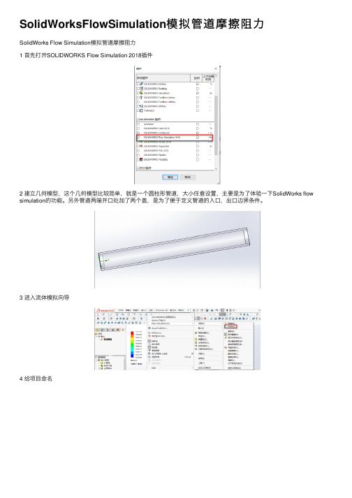
SolidWorksFlowSimulation模拟管道摩擦阻⼒
SolidWorks Flow Simulation模拟管道摩擦阻⼒
1 ⾸先打开SOLIDWORKS Flow Simulation 2018插件
2 建⽴⼏何模型,这个⼏何模型⽐较简单,就是⼀个圆柱形管道,⼤⼩任意设置,主要是为了体验⼀下SolidWorks flow simulation的功能。
另外管道两端开⼝处加了两个盖,是为了便于定义管道的⼊⼝,出⼝边界条件。
3 进⼊流体模拟向导
4 给项⽬命名
5 单位系统选择默认SI单位制
6 因为是内流场分析,这⾥选择内部,物理特征不涉及,不管
7 流体这⾥选择液体⽔,双击,流动类型为仅湍流。
8 这⾥保持默认,光滑壁⾯。
9 这⾥修改湍流强度和湍流长度。
10 完成之后会⾃动⽣成计算域,点击计算域右键选择隐藏
11 点击边界条件,右键插⼊边界条件,选择左边盖⼦的内表⾯,选择⼊⼝速度为10m/s,勾选充分发展流动,表明为完全发展的湍流。
12 再次点击边界条件,右键插⼊边界条件,选择右边盖⼦的内表⾯,选择静压1atm,即101325pa
Ps:假如内表⾯因为遮挡不好选定,可将管⼦和计算域隐藏再选择。
13 然后点击⽬标,右键选择插⼊表⾯⽬标,同样假如有遮挡,可以先把盖⼦隐藏再选定
14 选择⽹格,右键选择全局⽹格,保持默认⽹格划分就⾏,这⾥⼏何不复杂。
最后右键点击管道摩擦项⽬名称,点击运⾏,运⾏,⼀会就可以看到结果
15 切⾯结果(选择结果-切⾯图-右键插⼊)
16 查看⽬标值(选择结果-⽬标图-右键插⼊-显⽰)。
如何使用SolidWorksFlowSimulation进行流体分析
如何使用SolidWorksFlowSimulation进行流体分析如何使用SolidWorks Flow Simulation进行流体分析第一章介绍SolidWorks Flow Simulation软件SolidWorks Flow Simulation是一款功能强大的流体分析软件,可用于研究和模拟各种流体行为,如流动、传热以及过程优化。
本章将介绍SolidWorks Flow Simulation的基本概念和软件界面。
1.1 SolidWorks Flow Simulation概述SolidWorks Flow Simulation是一款基于计算流体力学(CFD)原理的流体分析软件。
它提供了一种直观且易于使用的界面,使用户能够轻松地进行流体分析。
该软件适用于涉及空气、液体和气体等多种流体的工程领域,如航空航天、汽车、建筑、能源等。
1.2 SolidWorks Flow Simulation软件界面SolidWorks Flow Simulation软件的界面分为几个主要的模块,包括模型准备、模拟设定、网格划分、求解器设置和结果分析。
在模型准备模块中,用户可以导入、创建和编辑三维模型。
在模拟设定模块中,用户可以设置流体的边界条件、流体材料属性和求解器选项。
在网格划分模块中,用户可以对模型进行网格划分以提高计算精度。
在求解器设置模块中,用户可以选择不同的求解器和求解算法。
在结果分析模块中,用户可以对流体的流速、压力、温度等进行可视化和分析。
第二章 SolidWorks Flow Simulation基本操作本章将介绍使用SolidWorks Flow Simulation进行流体分析的基本操作,包括创建流体域、设置边界条件、定义流体材料和运行求解器。
2.1 创建流体域在使用SolidWorks Flow Simulation进行流体分析之前,首先需要创建定义流体域的模型。
用户可以使用SolidWorks CAD软件创建三维模型,然后导入到Flow Simulation中。
FlowSimulation网格划分技术简介
FlowSimulation网格划分技术简介Flow Simulation的网格技术Flow Simulation是以SolidWorks作为平台的CFD分析软件,它与其他主流的CFD分析软件一样,采用有限体积法。
即将计算区域划分为一系列不重复的控制体积,并使每个网格点周围有一个控制体积;将待解的建立在流体动力学现象的微分方程对每一个控制体积积分,便得出一组离散方程。
这个控制体积可以简单的理解为网格。
划分网格是CDF分析中比较关键的一步,它关系到分析结果的精度。
这就值得我们去讨论Flow Simulation的网格技术了。
一网格的要求和选择我们在做任何CFD分析,都要对计算区域进行离散,即划分网格。
网格是CFD 模型的几何表达形式,也是模拟与分析的载体。
网格质量对CFD计算精度和计算效率有很大的影响。
因此,我们对网格的划分要有足够的关注。
1 网格排列网格分为结构网格和非结构网格两大类。
结构网格即网格中节点排列有序、邻点间的关系明确,如图1所示。
图1 结构网格与结构网格不同,在非结构网格中,节点的位置无法用一个固定的法则予以有序地命名。
图2是非结构网格示例。
这种网格虽然生成过程比较复杂,但却有着极好的适应性,尤其对具有复杂边界的流场计算问题特别有效。
非结构网格一般通过专门的程序或软件来生成。
另外,在某一区域内结构化网格与其它结构化网格以某种方式结合的网格,这种网格成为部分非结构化网格。
图2 非结构网格2 网格单元的分类单元是构成网格的基本元素。
在结构网格中,常用的2D网格单元是四边形单元,3D网格单元是六面体单元。
而在非结构网格中,常用的2D网格单元还有三角形单元,3D网格单元还有四面体单元和五面体单元,其中五面体单元还可分为棱锥形(或楔形)和金字塔形单元等。
图3和图4分别示出了常用的2D和3D网格单元。
图3 常用的2D网格单元图4常用的3D网格单元另外,立方体形式的六面体网格,其网格面与笛卡儿坐标系中的X、Y、Z 轴相平行。
solidworksflowsimulation操作方法

solidworksflowsimulation操作方法SolidWorks Flow Simulation 是一款流体力学分析软件,它可以帮助用户模拟和优化涉及流体流动、传热和流体力学等方面的工程问题。
以下是 SolidWorks Flow Simulation 的操作方法详解,包括设置分析类型、创建流体域、定义边界条件、运行计算并分析结果等步骤。
1. 启动 SolidWorks,并打开要进行流体力学分析的模型。
2. 在 SolidWorks 菜单栏中选择 "工具"(Tools),再选择 "流体力学"(Flow Simulation)。
3. 在弹出的 "流体力学属性管理器"(Flow Simulation PropertyManager)中,选择 "新建项目"(New Project)。
4. 在 "项目名称"(Project Name)栏中输入项目名称,并选择 "测量单位"(Units)和 "流体"(Fluid)类型。
5. 在 "分析类型"(Analysis Type)中设置要进行的流体力学分析类型,如内部流动(Internal Flow)、外部流动(External Flow)或热传导(Heat Transfer)。
6. 在 "流体域"(Fluid Domain)中设置分析的流体域。
可以直接在三维模型上进行选择,也可以手动定义流体域的形状和尺寸。
7. 在 "材料属性"(Material Properties)中设置流体的物理性质,如密度、粘度和热导率等。
8. 在 "边界条件"(Boundary Conditions)中定义边界条件,包括进口流量、出口压力、壁面温度等。
可以直接在模型上选择相应的面或体进行设置。
sw flow simulation使用简介及流体力学热力学基础

热现象:传导 对流 辐射
SW flow simulation 设计更好的产品
CFD结果导入CAE
非牛顿流体
电子设备热分析 风扇曲线 旋转区域:全体or局部
优化设计-参数分析
SW flow simulation,一款易用但功能强大的CFD仿真软件,包括但不限于上述应用……
2014/12/13 6
SW flow simulation 使用简介
2014/12/13
15Biblioteka SW flow simulation 使用简介
网格划分: sw根据通过使用整个模型的所有尺寸、计算域 及指定了边界条件和目标的面组来计算默认的 minimum gap size 和minimum wall thickness。 如右图这个算例,0.1524m就是出口的宽度。(选 中手动设置,下方会出现数值,可以认为这个数字 是系统的默认值,显然需要修改这个数值,系统不 足以识别小间隙和薄壁) 当添加了另一个边界条件后,可以看出默认的最 小gap size已经变成小圆孔的直径了。总数接近 60w个网格。计算机难以计算。
2014/12/13
19
SW flow simulation 使用简介
网格划分: 在没有实体存在的区域细分网格或者设置目标,需要创建一个包围此区域的零件,以表 明关注的区域。然后再使用“零部件控制”命令将此零件禁用。 使用“局部初始网格”命令时,要在设计树中选中这个零件名称,如果在主窗口中点选 这个零件实体,软件会认为是使用这个零件的外表面来作为细化区域。 “优化薄壁面求解”可以在算法上解析薄壁特征,而不 需要对薄壁周围进行任何形式的网格细化。薄壁的两个面 可能都位于同一个单元内,如果两侧流速不同,或者考虑固 体壁导热,这样粗的网格是不可以接受的。使用了这个选项 则可以正确处理,没必要生成更多网格来解析细小特征。 总结: 1、自动网格适用于绝大多数模型,但是当模型含有多个区域需要不同的网格设置时, 自动划分会数量偏多,当计算变得很慢时,请改为手动设置。 2、一套有质量的网格划分不仅需要对模型几何体正确剖析,也需要对流动特性精确剖 析。 3、有时一套适用的网格是很难得到的,常用方法就是试错法。 4、仿真的结果精度很大程度取决于网格质量,多花点时间放在手动设置网格上,会计 算的又快又准。
solidworks流体分析
solidworks流体分析
学习流体分析——SolidWorks FloXpress
ICT-Lenny
SolidWorks FloXpress 为定性流量分析工具,它的操作简单,并且易学易用。
只要工程师对流体有一点
基础了解,就可以利用SolidWorks FloXpress进行分析,不要求工程师们有很强的专业知识。
它是一款免费挂在SolidWorks上的插件,可以对单个出入口的模型进行流体分析,让您洞察您的SolidWorks 模型中的水或空气流动。
如果要您要做更加复杂的流体分析,则需要利用SolidWorks Flow Simulation 。
SolidWorks Flow Simulation包括有一系列气体、液体、可压缩液体、非牛顿液体、真实气体、蒸汽,以及生成自定义流体的能力。
SolidWorks Flow Simulation还可以轻易地对多个出入口的复杂模型进行流体分析。
下面,我将对SolidWorks FloXpress的使用做一个详细的阐述。
首先打开将要进行分析的模型。
此模型是一个阀体,如下图:拿到模型后,第一步是先将阀体的两个端口封闭。
如果不封闭FloXpress将无法进行运算
接下来,可以进行流体分析了。
floefd flow simulation (7)工具
工具 -概述在 Flow Simulation 中可使用下列工具:相关性用于以合适的方式指定数据: 用作常数,用作表或公式对x 、y 、z 、半径(r ), phi (j )、theta (q ) 坐标和时间t (仅用于分析)。
半径是点到从参考坐标系所选的参考轴的距离。
对于在和中指定的值,应用。
半径、phi 和 theta 坐标形成球形坐标系,其中点到参考坐标系原点的距离(R ) 通过半径(r ) 和 theta (q ) 定义,如下所示: r=R·cos (q )。
有关详细信息,请参阅。
对于表面热源和体积热源,您还可以在项目中指定对任何目标的相关性。
l 常数。
指定的值是常数。
这是所有条目的默认选项,除了切换。
l表。
通过它可以用表指定与坐标相关或随时间变化的参数(风扇和热源仅可随时间变化)。
您可以用以下某种方式指定表相关性:l随一个参数变化的表。
通过它可以指定基于以下某个坐标的表相关性: x 、y 、z 、半径、phi 、theta 或时间t (仅用于分析);l随笛卡尔坐标和时间变化的表。
通过它可以指定或参数基于笛卡尔坐标(x、y、z )和时间t (仅用于分析)的表相关性。
l随目标变化的表。
通过它可以为或参数指定基于目标值的表相关性。
对于所有类型的表相关性,值表中的自变量值必须以升序排列(最小值在顶部,表格越往下值越大)。
指定表相关性后,您可以从Microsoft Excel 导入数据: 在 Excel 工作表中定义一个两列表,将表复制到剪切板,然后在值表中单击任意自变量(左)网格,然后按 Ctrl+V 或右键单击该网格并选择粘贴将数据粘贴到表中。
还可以将值表导出到 Excel 工作表中: 按住 Shift ,然后单击要导出的网格。
按 Ctrl+C 或右键单击选定网格并选择复制,将网格的内容复制到粘贴板,然后打开Excel 文档,将数据粘贴到网格中。
l公式定义。
通过它可以指定公式相关性。
- 1、下载文档前请自行甄别文档内容的完整性,平台不提供额外的编辑、内容补充、找答案等附加服务。
- 2、"仅部分预览"的文档,不可在线预览部分如存在完整性等问题,可反馈申请退款(可完整预览的文档不适用该条件!)。
- 3、如文档侵犯您的权益,请联系客服反馈,我们会尽快为您处理(人工客服工作时间:9:00-18:30)。
EDB: 导热胶材料库 Libraries – Interface Materials (Electronics module)
导热胶材料库:Bergquist, Chomerics, Dow Corning and Thermagon. 通常很难获取,这些数据都比较真实.
Confidential Information
Confidential Information
Libraries – Fans (Electronics module)
Confidential Information
Libraries – 2R Components (Electronics module)
支持标准. 支持封装类型: CBGA, Chip Array, LQFP, MQFP, PBGA, PLCC, QFN, SOP, SSOP, TQFP, TSOP, TSSOP
解决方案:
采用FloFlow Simulation进行分析 通过大量的―what-if‖ 分析将温升降到最低
好处:
建立有记录的优化设计方案
Confidential Information
Electronics Module – Proven in the real world
AP Labs 重新设计(电器或电子设备的 )支架装置及封装
Confidential Information
PMV
PMV值是丹麦的范格尔(P.O.Fange的冷热感觉的平均。PMV = 0时意味着室内热环境 为最佳热舒适状态。ISO7730对PMV的推荐值为PMV 值 在= -0.5~+0.5之间。 PMV指数可通过估算人体活动的代谢率及服装的隔 热值获得,同时还需有以下的环境参数:空气温度、平均 辐射温度、相对空气流速及空气湿度。 PMV指数是根据人体热平衡计算的。当人体内部产 生的热等于在环境中散失的热量时,人处于热平衡状态。
Electronics Module – Proven in the real world
Sharp 试验室采用FloFlow Simulation 进行 LCD优化
优化LCD模块用于不同的应用; 好处:
分析结果轻松生成 在设计团队内进行技术改进沟通
Confidential Information
• 实体的扩展数据库 • 包含以下材料类型的完整的数据库: • 合金、陶瓷、玻璃、矿产品、金属、高 分子材料、半导体
Confidential Information
建筑及土木材料库
Confidential Information
Confidential Information
简介
Electronics cooling模块 是Flow Simuklation针对电子 散热分析领域的“升级”模块. 本次版本引入了针对电子部件和工程库的核心改进.
Confidential Information
Electronics特性列表
2010版本 风扇 散热片 热源 热电致冷器(TEC) 辐射 多孔散热板 工程数据库(数量有限) 2011 焦耳热 2-R模型 热管 PCB生成器(印刷电路板) 完整的数据库
Joule Heating - 2 (Electronics module)
优势:
•在汽车和能源电子许多应用方面提供一个解决方案, 其中焦耳热影响是一关 键的物理过程(如电动马达单元或功率分布架). •容许精确的模拟计算的电损耗热(如电子转换的载荷损失). •为满足模拟PCB走线的焦耳热影响的需求提供了一个解决方案。
•对客户直觉上很吸引 •他们基于JEDEC(固态技术协会) 标准做过测试. •他们提供可以接受的结果精度. •与传统的单热阻处理方法相比,这 种方法是个很大的改进. •Flow Simulation中有丰富的双热阻 模型库支持(JEDEC标准)
Confidential Information
焦耳热
Confidential Information
热管简介
Confidential Information
热管简化模型(Electronics module)
特性:
•代表热管,需要指定热管整体有效热阻,制定热流进出口面. •热管性能取决于许多因素, 如斜度, 方向, 长度等. 用户可以通过指定不同的有效热阻模 型不同的条件.
Confidential Information
预计不满意者的百分数(PPD)
PPD指数为预计处于热环境中的群体对于热环境不满意的 投票平均值。 PPD指数可预计群体中感觉过暖或过凉“根据七级热感觉 投票表示热(+3),温暖(+2),凉(-2)或冷(-3)” 的人的百分数。
Confidential Information
空气分布特性指标ADPI
该指标综合考虑了空气温度、气流速度和人的舒适度三方 面的因素。 如果ADPI=100%,表示全室人员都感到舒适; ADPI达到80%,即可认为是满意的气流组织效果。
Confidential Information
Library - Building Materials (HVAC module)
2—R器件 多孔板 风扇 TEC 电子固体 导热胶 ~
Confidential Information
双热阻部件简化模型(Electronics module) •优势: •特性:
•双热阻部件简化模型针对电子封装 模拟. •需要预定义:结-壳热阻(Rjc)和结 -板热阻(Rjb). •Flow Simulation中封装几何由两个 板型固体组成,分别代表结与壳, 双 热阻模型将热阻数据分别应用上去.
Flow Simulation 2011 新模块 上海雷瓦
Confidential Information
Flow Simulation 2011 新模块
Electronic Cooling 电子冷却
HVAC 设计
Confidential Information
Electronic Cooling module 电子冷却专业模块
挑战:
允许足够的空气流动
– 不够的的空气流动会使昂贵的VME卡不可靠
解决方案:
采用―what-if‖ 的设计分析
好处:
总体上,通过卡的空气流动性能增加27% 最关键的4个插槽流动性能增加40 尽管减少了一半的风扇,但整个系统的平均故 障时间增加 (MTBF
Confidential Information
电子散热实例
Confidential Information
Electronics Module – Proven in the real world
NEC Develops SX Series of Supercomputers超级计算机
挑战:
保证具有非常紧凑结构的新设计具有良好的散 热性能 在此之前使用传统CFD分析,非常不成功(时间 周期很长、需要硕士以上学历的专业分析人员)
特性:
•现在可以计算稳态、导电固体的直流发热. •相关的焦耳热特定影响自动计算包括传热计算. •材料电阻可以是各向同性或者是各向异性的或 者与温度相关的. •电动势和电流计算只在传导固体中计算 •如金属与复合金属材料. –绝缘体, 半导体, 流体以及真空区域不参与计算.
Confidential Information
采暖通风和空调模块(HVAC)
高级辐射模型 舒适度参数 材料库更新
Confidential Information
高级辐射模型
• 半透明实体(实体吸收辐射) • 依赖于光波长度 • 光谱定义 • Specularity of surfaces • 折射率 • 辐射源特征
Confidential Information
• Large database of building materials
Confidential Information
Libraries – Fans (HVAC module)
• Additional database of Fans
Confidential Information
Libraries – Solid Materials (HVAC module)
Confidential Information
Libraries – TECs (Electronics module)
Support for Marlow and Melcor parts.
Confidential Information
EDB: 电子固体材料库(Electronics module)
典型电子系统设计所需材料. 包括的材料有:Alloys, Ceramics, Glasses & Minerals, Laminates, Metals, Polymers and Semiconductors. 为典型的IC封装提供特殊的单热 阻库.
Confidential Information
特性:
•得到两个方向的导热系数、法向和层内 导热系数. •PCB可以是任意方向;如:斜置板.
Confidential Information
PCB Generator - 2 (Electronics module)
优势:
•简单而又标准的方法决定多层PCB板特性. •任意放置的PCB使得简单而准确的模拟以一定角度布置的双列直插式内存(DIMM).
Confidential Information
Libraries (Electronics module)
特性
•加入了大量新的固体材料,风扇,TEC, 双热阻部件库; •增加了导热胶材料库; •增加了代表IC封装的单块库,提供有效 密度,有效导热系数;
优势
•用户可以直接获取预定义的与电子部件 相关的有效特性; •库还可以扩展; •对电子散热分析很有用;