tensorflow用CNN训练和测试mnist手写数字识别程序代码
tensorflow学习笔记——使用TensorFlow操作MNIST数据(1)

tensorflow学习笔记——使⽤TensorFlow操作MNIST数据(1) 续集请点击我: 本节开始学习使⽤tensorflow教程,当然从最简单的MNIST开始。
这怎么说呢,就好⽐编程⼊门有Hello World,机器学习⼊门有MNIST。
在此节,我将训练⼀个机器学习模型⽤于预测图⽚⾥⾯的数字。
开始先普及⼀下基础知识,我们所说的图⽚是通过像素来定义的,即每个像素点的颜⾊不同,其对应的颜⾊值不同,例如⿊⽩图⽚的颜⾊值为0到255,⼿写体字符,⽩⾊的地⽅为0,⿊⾊为1,如下图。
MNIST 是⼀个⾮常有名的⼿写体数字识别数据集,在很多资料中,这个数据集都会被⽤做深度学习的⼊门样例。
⽽Tensorflow的封装让MNIST数据集变得更加⽅便。
MNIST是NIST数据集的⼀个⼦集,它包含了60000张图⽚作为训练数据,10000张图⽚作为测试数据。
在MNIST数据集中的每⼀张图⽚都代表了0~9中的⼀个数字。
图⽚的⼤⼩都为28*28,且数字都会出现在图⽚的正中间,如下图: 在上图中右侧显⽰了⼀张数字1的图⽚,⽽右侧显⽰了这个图⽚所对应的像素矩阵,MNIST数据集提供了四个下载⽂件,在tensorflow中可以将这四个⽂件直接下载放到⼀个⽬录中并加载,如下代码input_data.read_data_sets所⽰,如果指定⽬录中没有数据,那么tensorflow 会⾃动去⽹络上进⾏下载。
下⾯代码介绍了如何使⽤tensorflow操作MNIST数据集。
MNIST数据集的官⽹是。
在这⾥,我们提供了⼀份python源代码⽤于⾃动下载和安装这个数据集。
你可以下载,然后⽤下⾯的代码导⼊到你的项⽬⾥⾯,也可以直接复制粘贴到你的代码⽂件⾥⾯。
注意:MNIST数据集包括训练集的图⽚和标记数据,以及测试集的图⽚和标记数据,在测试集包含的10000个样例中,前5000个样例取⾃原始的NIST训练集,后5000个取⾃原始的NIST测试集,因此前5000个预测起来更容易些。
Tensorflow2.0多层感知机实现mnist手写数字识别
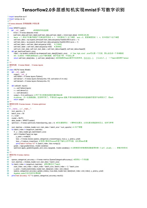
Tensorflow2.0多层感知机实现mnist⼿写数字识别 1import tensorflow as tf2import numpy as np3"""4tf.keras.datasets 获得数据集并预处理5"""6class MNISTLoader():7def__init__(self): #加载类的构造函数8 mnist = tf.keras.datasets.mnist9 (self.train_data,self.train_label),(self.test_data,self.test_label) = mnist.load_data() #(6000,28,28)10#axis = 1 ,相当于在最内层每个元素加括号变成 n, 1 ,在后⾯加个1 这个维度; axis = 0,就是维度变成 1,n,在中间加个1这个维度11 self.train_data = np.expand_dims(self.train_data.astype(np.float32)/255.0,axis = -1)12 self.test_data = np.expand_dims(self.test_data.astype(np.float32)/255.0,axis = -1)13 self.test_label = self.test_label.astype(np.int32) # [10000]14 self.train_label = self.train_label.astype(np.int32) # [60000]15 self.num_train_data, self.num_test_data = self.train_data.shape[0], self.test_data.shape[0]16def get_batch(self,betch_size):17 index = np.random.randint(0,np.shape(self.train_data)[0],batch_size) #(low, high, size),size可以是⼀个元组,那么会⽣成⼀个多维数组18#从(0,6000)中随机抽取batch_size个随机整数,数字包括下界,不包括上界19return self.train_data[index, :], self.train_label[index] #返回抽取的batch数字对应的样本,[[],[],[],[],...], [1,3,4,5,7,...] ⼀个batch返回两个tensor 2021"""22模型构建,tf.keras.Model ,yers23"""24class MLP(tf.keras.Model):25def__init__(self):26 super().__init__()27 self.flatten = yers.Flatten()28 self.dense1 = yers.Dense(units=100, activation=tf.nn.relu)29 self.dense2 = yers.Dense(units=10)3031def call(self, inputs):32 x = self.flatten(inputs)33 x = self.dense1(x)34 x = self.dense2(x)35 output = tf.nn.softmax(x) # ⽤了多分类激活函数在最后输出层36# softmax,归⼀化指数函数。
python,tensorflow,CNN实现mnist数据集的训练与验证正确率

python,tensorflow,CNN实现mnist数据集的训练与验证正确率1.⼯程⽬录2.导⼊data和input_data.pyN.pyimport tensorflow as tfimport matplotlib.pyplot as pltimport input_datamnist = input_data.read_data_sets('data/', one_hot=True)trainimg = mnist.train.imagestrainlabel = belstestimg = mnist.test.imagestestlabel = belsprint('MNIST ready')n_input = 784n_output = 10weights = {'wc1': tf.Variable(tf.truncated_normal([3, 3, 1, 64], stddev=0.1)),'wc2': tf.Variable(tf.truncated_normal([3, 3, 64, 128], stddev=0.1)),'wd1': tf.Variable(tf.truncated_normal([7*7*128, 1024], stddev=0.1)),'wd2': tf.Variable(tf.truncated_normal([1024, n_outpot], stddev=0.1)),}biases = {'bc1': tf.Variable(tf.random_normal([64], stddev=0.1)),'bc2': tf.Variable(tf.random_normal([128], stddev=0.1)),'bd1': tf.Variable(tf.random_normal([1024], stddev=0.1)),'bd2': tf.Variable(tf.random_normal([n_outpot], stddev=0.1)),}def conv_basic(_input, _w, _b, _keepratio):_input_r = tf.reshape(_input, shape=[-1, 28, 28, 1])_conv1 = tf.nn.conv2d(_input_r, _w['wc1'], strides=[1, 1, 1, 1], padding='SAME')_conv1 = tf.nn.relu(tf.nn.bias_add(_conv1, _b['bc1']))_pool1 = tf.nn.max_pool(_conv1, ksize=[1, 2, 2, 1], strides=[1, 2, 2, 1], padding='SAME')_pool_dr1 = tf.nn.dropout(_pool1, _keepratio)_conv2 = tf.nn.conv2d(_pool_dr1, _w['wc2'], strides=[1, 1, 1, 1], padding='SAME')_conv2 = tf.nn.relu(tf.nn.bias_add(_conv2, _b['bc2']))_pool2 = tf.nn.max_pool(_conv2, ksize=[1, 2, 2, 1], strides=[1, 2, 2, 1], padding='SAME')_pool_dr2 = tf.nn.dropout(_pool2, _keepratio)_densel = tf.reshape(_pool_dr2, [-1, _w['wd1'].get_shape().as_list()[0]])_fc1 = tf.nn.relu(tf.add(tf.matmul(_densel, _w['wd1']), _b['bd1']))_fc_dr1 = tf.nn.dropout(_fc1, _keepratio)_out = tf.add(tf.matmul(_fc_dr1, _w['wd2']), _b['bd2'])out = {print('CNN READY')x = tf.placeholder(tf.float32, [None, n_input])y = tf.placeholder(tf.float32, [None, n_output])keepratio = tf.placeholder(tf.float32)_pred = conv_basic(x, weights, biases, keepratio)['out']cost = tf.reduce_mean(tf.nn.softmax_cross_entropy_with_logits(_pred, y))optm = tf.train.AdamOptimizer(learning_rate=0.01).minimize(cost)_corr = tf.equal(tf.argmax(_pred, 1), tf.argmax(y, 1))accr = tf.reduce_mean(tf.cast(_corr, tf.float32))init = tf.global_variables_initializer()print('GRAPH READY')sess = tf.Session()sess.run(init)training_epochs = 15batch_size = 16display_step = 1for epoch in range(training_epochs):avg_cost = 0.total_batch = 10for i in range(total_batch):batch_xs, batch_ys = mnist.train.next_batch(batch_size)sess.run(optm, feed_dict={x: batch_xs, y: batch_ys, keepratio: 0.7})avg_cost += sess.run(cost, feed_dict={x: batch_xs, y: batch_ys, keepratio: 1.0})/total_batch if epoch % display_step == 0:print('Epoch: %03d/%03d cost: %.9f' % (epoch, training_epochs, avg_cost))train_acc = sess.run(accr, feed_dict={x: batch_xs, y: batch_ys, keepratio: 1.})print('Training accuracy: %.3f' % (train_acc))res_dict = {'weight': sess.run(weights), 'biases': sess.run(biases)}import picklewith open('res_dict.pkl', 'wb') as f:pickle.dump(res_dict, f, pickle.HIGHEST_PROTOCOL)4.test.pyimport pickleimport numpy as npdef load_file(path, name):with open(path+''+name+'.pkl', 'rb') as f:return pickle.load(f)res_dict = load_file('', 'res_dict')print(res_dict['weight']['wc1'])index = 0import input_datamnist = input_data.read_data_sets('data/', one_hot=True)test_image = mnist.test.imagestest_label = belsimport tensorflow as tfdef conv_basic(_input, _w, _b, _keepratio):_input_r = tf.reshape(_input, shape=[-1, 28, 28, 1])_conv1 = tf.nn.conv2d(_input_r, _w['wc1'], strides=[1, 1, 1, 1], padding='SAME')_conv1 = tf.nn.relu(tf.nn.bias_add(_conv1, _b['bc1']))_pool1 = tf.nn.max_pool(_conv1, ksize=[1, 2, 2, 1], strides=[1, 2, 2, 1], padding='SAME')_pool_dr1 = tf.nn.dropout(_pool1, _keepratio)_conv2 = tf.nn.conv2d(_pool_dr1, _w['wc2'], strides=[1, 1, 1, 1], padding='SAME')_conv2 = tf.nn.relu(tf.nn.bias_add(_conv2, _b['bc2']))_pool2 = tf.nn.max_pool(_conv2, ksize=[1, 2, 2, 1], strides=[1, 2, 2, 1], padding='SAME')_pool_dr2 = tf.nn.dropout(_pool2, _keepratio)_densel = tf.reshape(_pool_dr2, [-1, _w['wd1'].shape[0]])_fc1 = tf.nn.relu(tf.add(tf.matmul(_densel, _w['wd1']), _b['bd1']))_fc_dr1 = tf.nn.dropout(_fc1, _keepratio)_out = tf.add(tf.matmul(_fc_dr1, _w['wd2']), _b['bd2'])out = {n_input = 784n_output = 10x = tf.placeholder(tf.float32, [None, n_input])y = tf.placeholder(tf.float32, [None, n_output])keepratio = tf.placeholder(tf.float32)_pred = conv_basic(x, res_dict['weight'], res_dict['biases'], keepratio)['out']cost = tf.reduce_mean(tf.nn.softmax_cross_entropy_with_logits(_pred, y))_corr = tf.equal(tf.argmax(_pred, 1), tf.argmax(y, 1))accr = tf.reduce_mean(tf.cast(_corr, tf.float32))init = tf.global_variables_initializer()sess = tf.Session()sess.run(init)training_epochs = 1batch_size = 1display_step = 1for epoch in range(training_epochs):avg_cost = 0.total_batch = 10for i in range(total_batch):batch_xs, batch_ys = mnist.train.next_batch(batch_size)if epoch % display_step == 0:print('_pre:', np.argmax(sess.run(_pred, feed_dict={x: batch_xs, keepratio: 1. }))) print('answer:', np.argmax(batch_ys))。
基于Tensorflow的MNIST手写数字识别分类
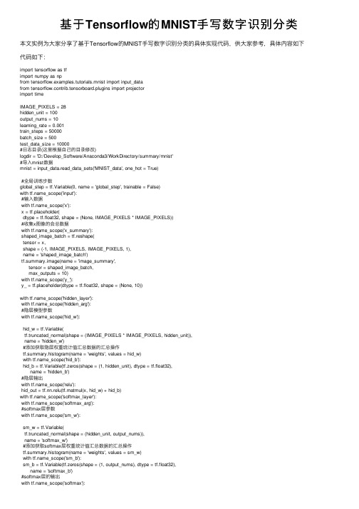
基于Tensorflow的MNIST⼿写数字识别分类本⽂实例为⼤家分享了基于Tensorflow的MNIST⼿写数字识别分类的具体实现代码,供⼤家参考,具体内容如下代码如下:import tensorflow as tfimport numpy as npfrom tensorflow.examples.tutorials.mnist import input_datafrom tensorflow.contrib.tensorboard.plugins import projectorimport timeIMAGE_PIXELS = 28hidden_unit = 100output_nums = 10learning_rate = 0.001train_steps = 50000batch_size = 500test_data_size = 10000#⽇志⽬录(这⾥根据⾃⼰的⽬录修改)logdir = 'D:/Develop_Software/Anaconda3/WorkDirectory/summary/mnist'#导⼊mnist数据mnist = input_data.read_data_sets('MNIST_data', one_hot = True)#全局训练步数global_step = tf.Variable(0, name = 'global_step', trainable = False)with _scope('input'):#输⼊数据with _scope('x'):x = tf.placeholder(dtype = tf.float32, shape = (None, IMAGE_PIXELS * IMAGE_PIXELS))#收集x图像的会总数据with _scope('x_summary'):shaped_image_batch = tf.reshape(tensor = x,shape = (-1, IMAGE_PIXELS, IMAGE_PIXELS, 1),name = 'shaped_image_batch')tf.summary.image(name = 'image_summary',tensor = shaped_image_batch,max_outputs = 10)with _scope('y_'):y_ = tf.placeholder(dtype = tf.float32, shape = (None, 10))with _scope('hidden_layer'):with _scope('hidden_arg'):#隐层模型参数with _scope('hid_w'):hid_w = tf.Variable(tf.truncated_normal(shape = (IMAGE_PIXELS * IMAGE_PIXELS, hidden_unit)),name = 'hidden_w')#添加获取隐层权重统计值汇总数据的汇总操作tf.summary.histogram(name = 'weights', values = hid_w)with _scope('hid_b'):hid_b = tf.Variable(tf.zeros(shape = (1, hidden_unit), dtype = tf.float32),name = 'hidden_b')#隐层输出with _scope('relu'):hid_out = tf.nn.relu(tf.matmul(x, hid_w) + hid_b)with _scope('softmax_layer'):with _scope('softmax_arg'):#softmax层参数with _scope('sm_w'):sm_w = tf.Variable(tf.truncated_normal(shape = (hidden_unit, output_nums)),name = 'softmax_w')#添加获取softmax层权重统计值汇总数据的汇总操作tf.summary.histogram(name = 'weights', values = sm_w)with _scope('sm_b'):sm_b = tf.Variable(tf.zeros(shape = (1, output_nums), dtype = tf.float32),name = 'softmax_b')#softmax层的输出with _scope('softmax'):y = tf.nn.softmax(tf.matmul(hid_out, sm_w) + sm_b)#梯度裁剪,因为概率取值为[0, 1]为避免出现⽆意义的log(0),故将y值裁剪到[1e-10, 1] y_clip = tf.clip_by_value(y, 1.0e-10, 1 - 1.0e-5)with _scope('cross_entropy'):#使⽤交叉熵代价函数cross_entropy = -tf.reduce_sum(y_ * tf.log(y_clip) + (1 - y_) * tf.log(1 - y_clip))#添加获取交叉熵的汇总操作tf.summary.scalar(name = 'cross_entropy', tensor = cross_entropy)with _scope('train'):#若不使⽤同步训练机制,使⽤Adam优化器optimizer = tf.train.AdamOptimizer(learning_rate = learning_rate)#单步训练操作,train_op = optimizer.minimize(cross_entropy, global_step = global_step)#加载测试数据test_image = mnist.test.imagestest_label = belstest_feed = {x:test_image, y_:test_label}with _scope('accuracy'):prediction = tf.equal(tf.argmax(input = y, axis = 1),tf.argmax(input = y_, axis = 1))accuracy = tf.reduce_mean(input_tensor = tf.cast(x = prediction, dtype = tf.float32))#创建嵌⼊变量embedding_var = tf.Variable(test_image, trainable = False, name = 'embedding') saver = tf.train.Saver({'embedding':embedding_var})#创建元数据⽂件,将MNIST图像测试集对应的标签写⼊⽂件def CreateMedaDataFile():with open(logdir + '/metadata.tsv', 'w') as f:label = np.nonzero(test_label)[1]for i in range(test_data_size):f.write('%d\n' % label[i])#创建投影配置参数def CreateProjectorConfig():config = projector.ProjectorConfig()embeddings = config.embeddings.add()embeddings.tensor_name = 'embedding:0'embeddings.metadata_path = logdir + '/metadata.tsv'projector.visualize_embeddings(writer, config)#聚集汇总操作merged = tf.summary.merge_all()#创建会话的配置参数sess_config = tf.ConfigProto(allow_soft_placement = True,log_device_placement = False)#创建会话with tf.Session(config = sess_config) as sess:#创建FileWriter实例writer = tf.summary.FileWriter(logdir = logdir, graph = sess.graph)#初始化全局变量sess.run(tf.global_variables_initializer())time_begin = time.time()print('Training begin time: %f' % time_begin)while True:#加载训练批数据batch_x, batch_y = mnist.train.next_batch(batch_size)train_feed = {x:batch_x, y_:batch_y}loss, _, summary= sess.run([cross_entropy, train_op, merged], feed_dict = train_feed) step = global_step.eval()#如果step为100的整数倍if step % 100 == 0:now = time.time()print('%f: global_step = %d, loss = %f' % (now, step, loss))#向事件⽂件中添加汇总数据writer.add_summary(summary = summary, global_step = step)#若⼤于等于训练总步数,退出训练if step >= train_steps:breaktime_end = time.time()print('Training end time: %f' % time_end)print('Training time: %f' % (time_end - time_begin))#测试模型精度test_accuracy = sess.run(accuracy, feed_dict = test_feed)print('accuracy: %f' % test_accuracy)saver.save(sess = sess, save_path = logdir + '/embedding_var.ckpt')CreateMedaDataFile()CreateProjectorConfig()#关闭FileWriterwriter.close()以上就是本⽂的全部内容,希望对⼤家的学习有所帮助,也希望⼤家多多⽀持。
分类-MNIST(手写数字识别)
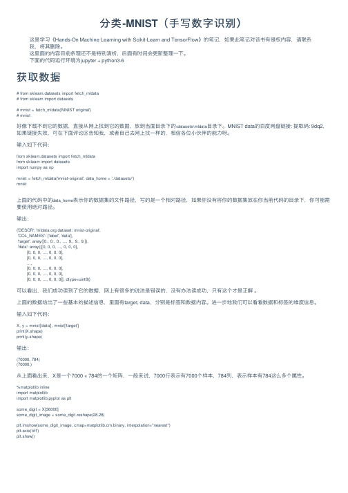
分类-MNIST(⼿写数字识别)这是学习《Hands-On Machine Learning with Scikit-Learn and TensorFlow》的笔记,如果此笔记对该书有侵权内容,请联系我,将其删除。
这⾥⾯的内容⽬前条理还不是特别清析,后⾯有时间会更新整理⼀下。
下⾯的代码运⾏环境为jupyter + python3.6获取数据# from sklearn.datasets import fetch_mldata# from sklearn import datasets# mnist = fetch_mldata('MNIST original')# mnist好像下载不到它的数据,直接从⽹上找到它的数据,放到当⾯⽬录下的\datasets\mldata⽬录下。
MNIST data的百度⽹盘链接: 提取码: 9dq2,如果链接失效,可在下⾯评论区告知我,或者⾃⼰去⽹上找⼀样的,相信各位⼩伙伴的能⼒呀。
输⼊如下代码:from sklearn.datasets import fetch_mldatafrom sklearn import datasetsimport numpy as npmnist = fetch_mldata('mnist-original', data_home = './datasets/')mnist上⾯的代码中的data_home表⽰你的数据集的⽂件路径,写的是⼀个相对路径,如果你没有将你的数据集放在你当前代码的⽬录下,你可能需要使⽤绝对路径。
输出:{'DESCR': ' dataset: mnist-original','COL_NAMES': ['label', 'data'],'target': array([0., 0., 0., ..., 9., 9., 9.]),'data': array([[0, 0, 0, ..., 0, 0, 0],[0, 0, 0, ..., 0, 0, 0],[0, 0, 0, ..., 0, 0, 0],...,[0, 0, 0, ..., 0, 0, 0],[0, 0, 0, ..., 0, 0, 0],[0, 0, 0, ..., 0, 0, 0]], dtype=uint8)}可以看出,我们成功读到了它的数据,⽹上有很多的说法是错误的,没有办法读成功,只有这个才是正解 。
基于TensorFlow框架的手写数字识别
基于TensorFlow框架的手写数字识别摘要:手写识别是一种应用在手机和平板电脑输入中的一种常见输入方式,目前国内已经有很多开源的机器学习平台可以方便的进行构建神经网络对手写数字进行识别。
如Google公司的TensorFlow和百度的PaddlePaddle(飞浆)。
本文通过搭建CNN卷积神经网络,利用python编程技术,使用TensorFlow框架并结合MNIST标准数据集对模型进行训练于评估,从而达到对手写数字的识别关键词:CNN卷积神经网络;TensorFlow;手写数字识别;数据集一.Tensorflow框架与MNIST数据集1.Tensorflow框架Google公司的Tensorflow深度学习框架是目前较为常用的深度学习平台。
Tensorflow框架的推出使人工智能的开发更加便捷。
Tensorflow支持多种CPU和GPU计算,可以很快的将神经网络计算部署到个人计算机和各类服务器上,也可支持多种模型训练。
例如卷积神经网络和递归神经网络。
在机器学习领域中使用的最常见的编程语言是python,python这一编程语言本身就集成了很多跟机器学习相关的第三方库,此外还有很多支持机器学习使用的库也可以很方便的导入到python中。
利用pip install tensorflow命令就可以将Tensorflow集成到python中。
1.MNIST数据集MNIST是一个非常有名的手写体数字识别数据集(手写数字灰度图像数据集),在很多资料中,这个数据集都会被用作深度学习的入门样例。
MNIST数据集是由0-9的数字图像构成的。
训练图像有6万张,测试图像有1万张。
MNIST数据集是MNIST数据集的一个子集,它包含了60000张图片作为训练数据,10000张图片作为测试数据。
由250个不同的人手写而成。
每一张图片都有对应的标签数字,训练图像一共有60000张,供研究人员训练出合适的模型。
测试图像一共有10000张,供研究人员测试训练的模型的性能。
tensorflow 训练 例程
tensorflow 训练例程
TensorFlow是一种强大的开源机器学习框架,提供了许多有用的工具和API来构建和训练深度神经网络。
以下是一些常见的TensorFlow训练例程。
1. MNIST手写数字识别:这是一个基本的图像分类问题,使用MNIST数据集。
该问题的目标是将手写数字图像分类为0到9之间的数字。
这个例子使用TensorFlow的卷积神经网络(CNN)来解决这个问题。
2. CIFAR-10图像分类:这是另一个图像分类问题,使用CIFAR-10数据集。
该问题的目标是将不同的图像分类为10个类别之一。
这个例子也使用了TensorFlow的CNN来解决这个问题。
3. 神经机器翻译:这是一个序列到序列的问题,使用一个神经网络将一种语言的句子翻译成另一种语言的句子。
这个例子使用了TensorFlow的循环神经网络(RNN)来解决这个问题。
4. TensorFlow对象检测API:这个API提供了一种易于使用的方法来训练和部署对象检测模型。
该API支持许多不同的模型架构,并提供了一个方便的图形用户界面来可视化训练过程。
以上是一些常见的TensorFlow训练例程,但还有许多其他的例子可以在TensorFlow官方文档中找到。
无论您是初学者还是有经验的开发人员,这些例子都可以帮助您更好地理解TensorFlow,并且在实践中获得更多的经验。
- 1 -。
tensorflow2 mnist训练代码
tensorflow2 mnist训练代码TensorFlow是一个流行的深度学习框架,广泛应用于机器学习和人工智能领域。
MNIST数据集是一个常用的手写数字识别数据集,本文将介绍如何使用TensorFlow2训练MNIST数据集。
一、准备工作首先,确保已经安装了TensorFlow2和相关依赖库。
可以使用以下命令在终端中安装TensorFlow:```shellpipinstalltensorflow```二、代码实现以下是一个简单的TensorFlow2代码示例,用于训练MNIST数据集:```pythonimporttensorflowastffromtensorflow.keras.datasetsimportmnistfromtensorflow.keras.modelsimportSequentialyersimportDense,Dropout,FlattenyersimportConv2D,MaxPooling2Dfromtensorflow.kerasimportbackendasK#加载MNIST数据集(x_train,y_train),(x_test,y_test)=mnist.load_data()#将像素值标准化为0到1之间的浮点数x_train=x_train/255.0x_test=x_test/255.0#将图像数据格式化为卷积神经网络输入格式img_rows,img_cols=28,28x_train=x_train.reshape(x_train.shape[0],img_rows,img_col s,1)x_test=x_test.reshape(x_test.shape[0],img_rows,img_cols,1) input_shape=(img_rows,img_cols,1)#将数据转换为适合TensorFlow模型的格式x_train=tf.convert_to_tensor(x_train,dtype='float32')y_train=tf.keras.utils.to_categorical(y_train,num_classes =10)x_test=tf.convert_to_tensor(x_test,dtype='float32')y_test=tf.keras.utils.to_categorical(y_test,num_classes=1 0)#创建模型model=Sequential()model.add(Conv2D(32,kernel_size=(3,3),activation='relu',i nput_shape=input_shape))model.add(MaxPooling2D(pool_size=(2,2)))model.add(Dropout(0.25))model.add(Flatten())model.add(Dense(128,activation='relu'))model.add(Dropout(0.5))model.add(Dense(num_classes,activation='softmax'))#编译模型pile(loss=tf.keras.losses.categorical_crossentro py,optimizer=tf.keras.optimizers.Adadelta(),metrics=['accurac y'])#训练模型model.fit(x=x_train,y=y_train,batch_size=128,epochs=10,ve rbose=1,validation_data=(x_test,y_test))```这段代码首先加载了MNIST数据集,并将像素值标准化。
深度学习基础-MNIST实验(tensorflow+CNN)
深度学习基础-MNIST实验(tensorflow+CNN)深度学习基础 - MNIST实验(Tensorflow-CNN)本⽂的完整代码托管在我的Github ,欢迎交流。
1.任务背景这⾥,我们拟通过搭建卷积神经⽹络(CNN)来完成⼿写数字识别任务,关于MNIST任务的相关内容可参考前⽂或。
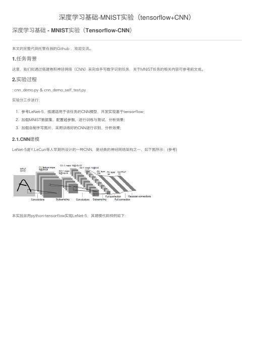
2.实验过程: cnn_demo.py & cnn_demo_self_test.py实验分三步进⾏:1. 参考LeNet-5,搭建适⽤于该任务的CNN模型,开发实现基于tensorflow;2. 加载MNIST数据集,配置超参数,进⾏训练与测试,分析效果;3. 加载⾃制⼿写图⽚,采⽤训练好的CNN进⾏识别,分析效果;N建模LeNet-5是Y.LeCun等⼈早期所设计的⼀种CNN,是经典的神经⽹络架构之⼀,如下图所⽰:(参考)本实验采⽤python-tensorflow实现LeNet-5,其建模代码样例如下:'''construction of leNet-5 model'''def lenet_5_forward_propagation(X):"""@note: construction of leNet-5 forward computation graph:CONV1 -> MAXPOOL1 -> CONV2 -> MAXPOOL2 -> FC3 -> FC4 -> SOFTMAX@param X: input dataset placeholder, of shape (number of examples (m), input size)@return: A_l, the output of the softmax layer, of shape (number of examples, output size)"""# reshape imput as [number of examples (m), weight, height, channel]X_ = tf.reshape(X, [-1, 28, 28, 1]) # num_channel = 1 (gray image)### CONV1 (f = 5*5*1, n_f = 6, s = 1, p = 'same')W_conv1 = weight_variable(shape = [5, 5, 1, 6])b_conv1 = bias_variable(shape = [6])# shape of A_conv1 ~ [m,28,28,6]A_conv1 = tf.nn.relu(tf.nn.conv2d(X_, W_conv1, strides = [1, 1, 1, 1], padding = 'SAME') + b_conv1)### MAXPOOL1 (f = 2*2*1, s = 2, p = 'same')# shape of A_pool1 ~ [m,14,14,6]A_pool1 = tf.nn.max_pool(A_conv1, ksize = [1, 2, 2, 1], strides=[1, 2, 2, 1], padding = 'SAME')### CONV2 (f = 5*5*1, n_f = 16, s = 1, p = 'same')W_conv2 = weight_variable(shape = [5, 5, 6, 16])b_conv2 = bias_variable(shape = [16])# shape of A_conv2 ~ [m,10,10,16]A_conv2 = tf.nn.relu(tf.nn.conv2d(A_pool1, W_conv2, strides = [1, 1, 1, 1], padding = 'VALID') + b_conv2)### MAXPOOL2 (f = 2*2*1, s = 2, p = 'same')# shape of A_pool2~ [m,5,5,16]A_pool2 = tf.nn.max_pool(A_conv2, ksize = [1, 2, 2, 1], strides=[1, 2, 2, 1], padding = 'SAME')### FC3 (n = 120)# flatten the volumn to vectorA_pool2_flat = tf.reshape(A_pool2, [-1, 5*5*16])W_fc3 = weight_variable([5*5*16, 120])b_fc3 = bias_variable([120])# shape of A_fc3 ~ [m,120]A_fc3 = tf.nn.relu(tf.matmul(A_pool2_flat, W_fc3) + b_fc3)### FC4 (n = 84)W_fc4 = weight_variable([120, 84])b_fc4 = bias_variable([84])# shape of A_fc4 ~ [m, 84]A_fc4 = tf.nn.relu(tf.matmul(A_fc3, W_fc4) + b_fc4)# Softmax (n = 10)W_l = weight_variable([84, 10])b_l = bias_variable([10])# shape of A_l ~ [m,10]A_l=tf.nn.softmax(tf.matmul(A_fc4, W_l) + b_l)return A_l2.2.训练与测试设置优化策略及相关超参数(如learning_rate、num_epochs、mini-batch size等),进⾏训练,经过⼀段时间的训练,得出的accuracy结果如下:Train Accuracy: 0.9920Valid Accuracy: 0.9896Test Accuracy: 0.9881同时该训练期间,指标accuracy和cost的变化过程如下图⽰:可以看出,此处CNN(LeNet-5)已经取得了不错的结果(≈99%的测试准确率)。
tensorflow基于CNN实战mnist手写识别(小白必看)
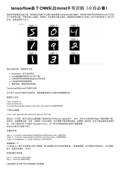
tensorflow基于CNN实战mnist⼿写识别(⼩⽩必看)很荣幸您能看到这篇⽂章,相信通过标题打开这篇⽂章的都是对tensorflow感兴趣的,特别是对卷积神经⽹络在mnist⼿写识别这个实例感兴趣。
不管你是什么基础,我相信,你在看完这篇⽂章后,都能够完全理解这个实例。
这对于神经⽹络⼊门的⼩⽩来说,简直是再好不过了。
通过这篇⽂章,你能够学习到tensorflow⼀些⽅法的⽤法mnist数据集的使⽤⽅法以及下载CNN卷积神经⽹络具体python代码实现CNN卷积神经⽹络原理模型训练、模型的保存和载⼊Tensorflow实战mnist⼿写数字识别关于这个mnist⼿写数字识别实战,我是跟着某课⽹上的教学视频跟着写的需要导⼊的包import numpy as npimport tensorflow as tffrom tensorflow.examples.tutorials.mnist import input_data #mnist数据⽤到的包下载mnist数据mnist = input_data.read_data_sets('mnist_data',one_hot=True)通过这⼀⾏代码,就可以将mnist数据集下载到本地⽂件夹mnist_data⽬录下,当然,你也可以使⽤绝对地址下载你想要下载的地⽅。
这⾥需要注意⼀点是,如果第⼀次运⾏程序,由于需要下载资源的缘故,故需要⼀段时间,并且下载过程是没有提⽰的,之后下载成功时才会提⽰ Success xxxxxx 。
另⼀种⽅式就是直接去官⽹下载数据集进去点击就可以直接下载了。
张量的声明input_x = pat.v1.placeholder(tf.float32,[None,28*28],name='input_x')#图⽚输⼊output_y = pat.v1.placeholder(tf.int32,[None,10],name='output_y')#结果的输出image = tf.reshape(input_x,[-1,28,28,1])#对input_x进⾏改变形状,稍微解释⼀下[-1,28,28,1] -1表⽰不考虑输⼊图⽚的数量,28*28是图⽚的长和宽的像素值,1是通道数量,由于原图⽚是⿊⽩的,所以通道是1,若是彩⾊图⽚,应为3.取测试图⽚和标签test_x = mnist.test.images[:3000]test_y = bels[:3000][:3000]表⽰从列表下标为0到2999 这些数据[1:3] 表⽰列表下标从1到2 这些数据卷积神经⽹络第⼀层卷积层(⽤最通俗的⾔语告诉你什么是卷积神经⽹络)#第⼀层卷积conv1 = yers.conv2d(inputs=image,#输⼊filters=32,#32个过滤器kernel_size=[5,5],#过滤器在⼆维的⼤⼩是5*5strides=1,#步长是1padding='same',#same表⽰输出的⼤⼩不变,因此需要补零activation=tf.nn.relu#激活函数)#形状[28,28,32]第⼆层池化层pool1 = yers.max_pooling2d(inputs=conv1,#第⼀层卷积后的值pool_size=[2,2],#过滤器⼆维⼤⼩2*2strides=2 #步长2)#形状[14,14,32]第三层卷积层2conv2 = yers.conv2d(inputs=pool1,filters=64,kernel_size=[5,5],strides=1,padding='same',activation=tf.nn.relu)#形状[14,14,64]第四层池化层2pool2 = yers.max_pooling2d(inputs=conv2,pool_size=[2,2],strides=2)#形状[7,7,64]平坦化flat = tf.reshape(pool2,[-1,7*7*64])使⽤flat.shape 输出的形状为(?, 3136)1024个神经元的全连接层dense = yers.dense(inputs=flat,units=1024,activation=tf.nn.relu)tf.nn.relu 是⼀种激活函数,⽬前绝⼤多数神经⽹络使⽤的激活函数是relu Droupout 防⽌过拟合dropout = yers.dropout(inputs=dense,rate=0.5)就是为了避免训练数据量过⼤,造成过于模型过于符合数据,泛化能⼒⼤⼤减弱。
tensorflow实现卷积神经网络经典案例--识别手写数字
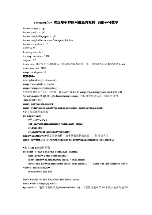
yotensorflow实现卷积神经网络经典案例--识别手写数字import numpy as npimport pandas as pdimport matplotlib.pyplot as pltimport matplotlib.cm as cm %matplotlib inlineimport tensorflow as tf#参数设置learning_rate=1e-4training_iterations=2000dropout=0.5batch_size=50 #所有的训练样本分批训练的效率最高,每一批的训练样本数量就是batch validation_size=2000image_to_display=10数据准备:data=pd.read_csv('.../train.csv')images=data.iloc[:,1:].valuesimages=images.astype(np.float)#对训练数据进行归一化处理,[0:255]=>[0.0:1.0] images=np.multiply(images,1.0/255.0)#print('images({0[0]},{0[1]})'.format(images.shape))可以查看数据格式,输出结果为'data(42000,784)'image_size=images.shape[1]image_width=image_height=np.ceil(np.sqrt(image_size)).astype(np.uint8)#定义显示图片的函数def display(img):#从784=>28*28one_img=img.reshape(image_width,image_height)plt.axis('off')plt.imshow(one_img,cmap=cm.binary)display(images[10]) #显示数据表格中第十条数据代表的数字,结果如下图labels_flat=data.iloc[:,0].values.ravel() labels_count=np.unique(labels_flat).shape[0]#定义one-hot编码函数def dense_to_one_hot(labels_dense, num_classes):num_labels = labels_dense.shape[0]index_offset = np.arange(num_labels) * num_classeslabels_one_hot = np.zeros((num_labels, num_classes)) labels_one_hot.flat[index_offset + labels_dense.ravel()] = 1return labels_one_hotlabels = dense_to_one_hot(labels_flat, labels_count)labels = labels.astype(np.uint8)#print(labels[10])的输出结果为'[0 0 0 0 0 0 0 0 1 0]',代表数据集中第10个数字的实际值为'8'#将数据拆分成用于训练和验证两部分validation_images=images[:validation_size]#将训练的数据分为train和validation,validation的部分是为了对比不同模型参数的训练效果,如:learning_rate, training_iterations, dropout validation_labels=labels[:validation_size]train_images = images[validation_size:]train_labels = labels[validation_size:]定义权重、偏差、卷积图层、池化图层:#定义weightdef weight_variable(shape):initial=tf.truncated_normal(shape,stddev=0.1)return tf.Variable(initial)#定义biasdef bias_variable(shape):initial=tf.constant(0.1,shape=shape)return tf.Variable(initial)#定义二维的卷积图层def conv2d(x,W):return tf.nn.conv2d(x,W,strides=[1,1,1,1],padding='SAME')#定义池化图层def max_pool_2x2(x): returntf.nn.max_pool(x,ksize=[1,2,2,1],strides=[1,2,2,1],padding='SAME')权重weight和偏置bias其实可以写成python的输入量,但是TensorFlow有更好的处理方式,将weight和bias设置成为变量,即计算图中的一个值,这样使得它们能够在计算过程中使用,甚至进行修改。
使用TensorFlow实现MNIST手写数字识别
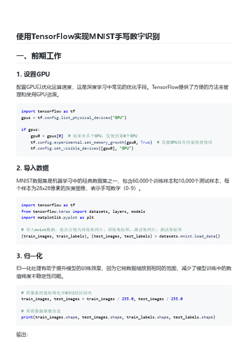
使用TensorFlow实现MNIST手写数字识别一、前期工作1. 设置GPU配置GPU以优化运算速度,这是深度学习中常见的优化手段。
TensorFlow提供了方便的方法来管理和使用GPU资源。
import tensorflow as tfgpus = tf.config.list_physical_devices("GPU")if gpus:gpu0 = gpus[0] # 如果有多个GPU,仅使用第0个GPUtf.config.experimental.set_memory_growth(gpu0, True) # 设置GPU显存用量按需使用tf.config.set_visible_devices([gpu0], "GPU")2. 导入数据MNIST数据集是机器学习中的经典数据集之一,包含60,000个训练样本和10,000个测试样本,每个样本为28x28像素的灰度图像,表示手写数字(0-9)。
import tensorflow as tffrom tensorflow.keras import datasets, layers, modelsimport matplotlib.pyplot as plt# 导入mnist数据,依次分别为训练集图片、训练集标签、测试集图片、测试集标签(train_images, train_labels), (test_images, test_labels) = datasets.mnist.load_data()3. 归一化归一化处理有助于提升模型的训练效果,因为它将数据缩放到相同的范围,减少了模型训练中的数值梯度不稳定性问题。
# 将像素的值标准化至0到1的区间内train_images, test_images = train_images /255.0, test_images /255.0# 查看数据维数信息print(train_images.shape, test_images.shape, train_labels.shape, test_labels.shape)输出:((60000, 28, 28), (10000, 28, 28), (60000,), (10000,))4. 数据可视化数据可视化有助于我们直观地理解数据分布和特征,确保数据加载和预处理过程的正确性。
三种方法实现MNIST手写数字识别

三种⽅法实现MNIST⼿写数字识别MNIST数据集下载:import tensorflow as tffrom tensorflow.examples.tutorials.mnist import input_datamnist = input_data.read_data_sets("MNIST_data/", one_hot=True) #one_hot 独热编码,也叫⼀位有效编码。
在任意时候只有⼀位为1,其他位都是0 1 使⽤逻辑回归:import tensorflow as tf# 导⼊数据集#from tensorflow.examples.tutorials.mnist import input_datamnist = input_data.read_data_sets("MNIST_data/", one_hot=True)# 变量batch_size = 50#训练的x(image),y(label)# x = tf.Variable()# y = tf.Variable()x = tf.placeholder(tf.float32, [None, 784])y = tf.placeholder(tf.float32, [None, 10])# 模型权重#[55000,784] * W = [55000,10]W = tf.Variable(tf.zeros([784, 10]))b = tf.Variable(tf.zeros([10]))# ⽤softmax构建逻辑回归模型pred = tf.nn.softmax(tf.matmul(x, W) + b)# 损失函数(交叉熵)cost = tf.reduce_mean(-tf.reduce_sum(y*tf.log(pred), 1))# 低度下降optimizer = tf.train.GradientDescentOptimizer(0.01).minimize(cost)# 初始化所有变量init = tf.global_variables_initializer()# 加载session图with tf.Session() as sess:sess.run(init)# 开始训练for epoch in range(25):avg_cost = 0.total_batch = int(mnist.train.num_examples/batch_size)for i in range(total_batch):batch_xs, batch_ys = mnist.train.next_batch(batch_size)sess.run(optimizer, {x: batch_xs,y: batch_ys})#计算损失平均值avg_cost += sess.run(cost,{x: batch_xs,y: batch_ys}) / total_batchif (epoch+1) % 5 == 0:print("Epoch:", '%04d' % (epoch+1), "cost=", "{:.9f}".format(avg_cost))print("运⾏完成")# 测试求正确率correct = tf.equal(tf.argmax(pred, 1), tf.argmax(y, 1))accuracy = tf.reduce_mean(tf.cast(correct, tf.float32))print("正确率:", accuracy.eval({x: mnist.test.images, y: bels}))结果:Extracting MNIST_data/train-images-idx3-ubyte.gzExtracting MNIST_data/train-labels-idx1-ubyte.gzExtracting MNIST_data/t10k-images-idx3-ubyte.gzExtracting MNIST_data/t10k-labels-idx1-ubyte.gzEpoch: 0005 cost= 0.394426425Epoch: 0010 cost= 0.344705163Epoch: 0015 cost= 0.323814137Epoch: 0020 cost= 0.311426675Epoch: 0025 cost= 0.302971779运⾏完成正确率: 0.91882 使⽤神经⽹络:import tensorflow as tfimport numpy as npfrom tensorflow.examples.tutorials.mnist import input_datadef init_weights(shape):return tf.Variable(tf.random_normal(shape, stddev=0.01))def model(X, w_h, w_o):h = tf.nn.sigmoid(tf.matmul(X, w_h)) # this is a basic mlp, think 2 stacked logistic regressionsreturn tf.matmul(h, w_o) # note that we dont take the softmax at the end because our cost fn does that for us mnist = input_data.read_data_sets("MNIST_data/", one_hot=True)trX, trY, teX, teY = mnist.train.images, bels, mnist.test.images, belsX = tf.placeholder("float", [None, 784])Y = tf.placeholder("float", [None, 10])w_h = init_weights([784, 625]) # create symbolic variablesw_o = init_weights([625, 10])py_x = model(X, w_h, w_o)cost = tf.reduce_mean(tf.nn.softmax_cross_entropy_with_logits(logits=py_x, labels=Y)) # compute coststrain_op = tf.train.GradientDescentOptimizer(0.05).minimize(cost) # construct an optimizerpredict_op = tf.argmax(py_x, 1)# Launch the graph in a sessionwith tf.Session() as sess:# you need to initialize all variablestf.global_variables_initializer().run()for i in range(100):for start, end in zip(range(0, len(trX), 128), range(128, len(trX)+1, 128)):sess.run(train_op, feed_dict={X: trX[start:end], Y: trY[start:end]})print(i, np.mean(np.argmax(teY, axis=1) ==sess.run(predict_op, feed_dict={X: teX})))结果:0 0.68981 0.82442 0.86353 0.8814 0.88815 0.89316 0.89727 0.90058 0.90429 0.90623 使⽤卷积神经⽹络:import tensorflow as tfimport numpy as npfrom tensorflow.examples.tutorials.mnist import input_databatch_size = 128test_size = 256def init_weights(shape):return tf.Variable(tf.random_normal(shape, stddev=0.01))def model(X, w, w2, w3, w4, w_o, p_keep_conv, p_keep_hidden):l1a = tf.nn.relu(tf.nn.conv2d(X, w, # l1a shape=(?, 28, 28, 32)strides=[1, 1, 1, 1], padding='SAME'))l1 = tf.nn.max_pool(l1a, ksize=[1, 2, 2, 1], # l1 shape=(?, 14, 14, 32)strides=[1, 2, 2, 1], padding='SAME')l1 = tf.nn.dropout(l1, p_keep_conv)l2a = tf.nn.relu(tf.nn.conv2d(l1, w2, # l2a shape=(?, 14, 14, 64)strides=[1, 1, 1, 1], padding='SAME'))l2 = tf.nn.max_pool(l2a, ksize=[1, 2, 2, 1], # l2 shape=(?, 7, 7, 64)strides=[1, 2, 2, 1], padding='SAME')l2 = tf.nn.dropout(l2, p_keep_conv)l3a = tf.nn.relu(tf.nn.conv2d(l2, w3, # l3a shape=(?, 7, 7, 128)strides=[1, 1, 1, 1], padding='SAME'))l3 = tf.nn.max_pool(l3a, ksize=[1, 2, 2, 1], # l3 shape=(?, 4, 4, 128)strides=[1, 2, 2, 1], padding='SAME')l3 = tf.reshape(l3, [-1, w4.get_shape().as_list()[0]]) # reshape to (?, 2048)l3 = tf.nn.dropout(l3, p_keep_conv)l4 = tf.nn.relu(tf.matmul(l3, w4))l4 = tf.nn.dropout(l4, p_keep_hidden)pyx = tf.matmul(l4, w_o)return pyxmnist = input_data.read_data_sets("MNIST_data/", one_hot=True)trX, trY, teX, teY = mnist.train.images, bels, mnist.test.images, bels trX = trX.reshape(-1, 28, 28, 1) # 28x28x1 input imgteX = teX.reshape(-1, 28, 28, 1) # 28x28x1 input imgX = tf.placeholder("float", [None, 28, 28, 1])Y = tf.placeholder("float", [None, 10])w = init_weights([3, 3, 1, 32]) # 3x3x1 conv, 32 outputsw2 = init_weights([3, 3, 32, 64]) # 3x3x32 conv, 64 outputsw3 = init_weights([3, 3, 64, 128]) # 3x3x32 conv, 128 outputsw4 = init_weights([128 * 4 * 4, 625]) # FC 128 * 4 * 4 inputs, 625 outputsw_o = init_weights([625, 10]) # FC 625 inputs, 10 outputs (labels)p_keep_conv = tf.placeholder("float")p_keep_hidden = tf.placeholder("float")py_x = model(X, w, w2, w3, w4, w_o, p_keep_conv, p_keep_hidden)cost = tf.reduce_mean(tf.nn.softmax_cross_entropy_with_logits(logits=py_x, labels=Y)) train_op = tf.train.RMSPropOptimizer(0.001, 0.9).minimize(cost)predict_op = tf.argmax(py_x, 1)# Launch the graph in a sessionwith tf.Session() as sess:# you need to initialize all variablestf.global_variables_initializer().run()for i in range(10):training_batch = zip(range(0, len(trX), batch_size),range(batch_size, len(trX)+1, batch_size))for start, end in training_batch:sess.run(train_op, feed_dict={X: trX[start:end], Y: trY[start:end],p_keep_conv: 0.8, p_keep_hidden: 0.5})test_indices = np.arange(len(teX)) # Get A Test Batchnp.random.shuffle(test_indices)test_indices = test_indices[0:test_size]print(i, np.mean(np.argmax(teY[test_indices], axis=1) ==sess.run(predict_op, feed_dict={X: teX[test_indices],Y: teY[test_indices],p_keep_conv: 1.0,p_keep_hidden: 1.0})))结果:0 0.94531251 0.97656252 0.99218753 0.988281254 0.9843755 0.99218756 0.9843757 0.99218758 0.988281259 0.99609375。
基于 CNN 的手写体数字识别系统的设计与实现代码大全

题目 基于CNN 的手写体数字识别系统的设计与实现(居中,宋体小三号,加粗)1.1 题目的主要研究内容(宋体四号加粗左对齐)(1)实验实验内容是通过CNN 模型实现对MNIST 数据集的手写数字识别,并通过GUI 界面进行演示,通过tensorflow 环境来构建模型并进行训练(2)系统流程图1.2 题目研究的工作基础或实验条件(1)硬件环境开始 获取数据集 构建CNN 模型 训练模型 搭建GUI 界面 测试结果结束Windows10系统(2)软件环境开发工具:python语言开发软件:pycharm开发环境:tensorflow1.3 数据集描述MNIST 是一个大型的、标准易用的、成熟的手写数字体数据集。
该数据集由不同人手写的0 至9 的数字构成,由60000 个训练样本集和10000 个测试样本集成,每个样本的尺寸为28x28x1,以二进制格式存储,如下图所示:1.4 特征提取过程描述CNN 是一种前馈型的神经网络,其在大型图像处理方面有出色的表现。
相比于其他神经网络结构,如多层感知机,卷积神经网络需要的参数相对较少(通过局部感受野和权值共享)。
CNN 的三个思想:局部感知野、权值共享、池化,能够大大简化权重参数的数量,网络的层数更深而参数规模减小,利于模型的训练。
CNN 主要包含三层:卷积层、池化层和全连接层,且在卷积层后应加入非线性函数作为激活函数,提高模型的非线性函数泛化能力,以下是单层CNN 的结构图:特征提取采用CNN模型中的卷积层,具体问为使用卷积核来进行特征提取。
1.5 分类过程描述分类过程采用全连接层和Softmax分类函数实现,通过softmax回归来输结果。
softmax模型可以用来给不同的对象分配概率。
对于输入的x加权求和,再分别i加上一个偏置量,最后再输入到softmax函数中,如下图。
其计算公式为:1.6 主要程序代码(要求必须有注释)import sys, ossys.path.append(os.pardir) # 为了导入父目录的文件而进行的设定import numpy as npimport matplotlib.pyplot as pltfrom dataset.mnist import load_mnistfrom simple_convnet import SimpleConvNetfrom common.trainer import Trainer# 读入数据(x_train, t_train), (x_test, t_test) = load_mnist(flatten=False)# 处理花费时间较长的情况下减少数据#x_train, t_train = x_train[:5000], t_train[:5000]#x_test, t_test = x_test[:1000], t_test[:1000]max_epochs = 20network = SimpleConvNet(input_dim=(1,28,28),conv_param = {'filter_num': 30, 'filter_size': 5, 'pad': 0, 'stride': 1},hidden_size=100, output_size=10, weight_init_std=0.01)trainer = Trainer(network, x_train, t_train, x_test, t_test,epochs=max_epochs, mini_batch_size=100,optimizer='Adam', optimizer_param={'lr': 0.001},evaluate_sample_num_per_epoch=1000)trainer.train()# 保存参数network.save_params("params.pkl")print("Saved Network Parameters!")# 绘制图形markers = {'train': 'o', 'test': 's'}x = np.arange(max_epochs)plt.plot(x, trainer.train_acc_list, marker='o', label='train', markevery=2)plt.plot(x, trainer.test_acc_list, marker='s', label='test', markevery=2)plt.xlabel("epochs")plt.ylabel("accuracy")plt.ylim(0, 1.0)plt.legend(loc='lower right')plt.show()MODE_MNIST = 1 # MNIST随机抽取MODE_WRITE = 2 # 手写输入Thresh = 0.5 # 识别结果置信度阈值# 读取MNIST数据集(_, _), (x_test, _) = load_mnist(normalize=True, flatten=False, one_hot_label=False)# 初始化网络# 网络1:简单CNN"""conv - relu - pool - affine - relu - affine - softmax"""network = SimpleConvNet(input_dim=(1,28,28),conv_param = {'filter_num': 30, 'filter_size': 5, 'pad': 0, 'stride': 1},hidden_size=100, output_size=10, weight_init_std=0.01) network.load_params("params.pkl")# 网络2:深度CNN# network = DeepConvNet()# network.load_params("deep_convnet_params.pkl")class MainWindow(QMainWindow,Ui_MainWindow):def __init__(self):super(MainWindow,self).__init__()# 初始化参数self.mode = MODE_MNISTself.result = [0, 0]# 初始化UIself.setupUi(self)self.center()# 初始化画板self.paintBoard = PaintBoard(self, Size = QSize(224, 224), Fill = QColor(0,0,0,0))self.paintBoard.setPenColor(QColor(0,0,0,0))self.dArea_Layout.addWidget(self.paintBoard)self.clearDataArea()# 窗口居中def center(self):# 获得窗口framePos = self.frameGeometry()# 获得屏幕中心点scPos = QDesktopWidget().availableGeometry().center() # 显示到屏幕中心framePos.moveCenter(scPos)self.move(framePos.topLeft())# 窗口关闭事件def closeEvent(self, event):reply = QMessageBox.question(self, 'Message',"Are you sure to quit?", QMessageBox.Yes |QMessageBox.No, QMessageBox.Y es)if reply == QMessageBox.Y es:event.accept()else:event.ignore()# 清除数据待输入区def clearDataArea(self):self.paintBoard.Clear()self.lbDataArea.clear()self.lbResult.clear()self.lbCofidence.clear()self.result = [0, 0]"""回调函数"""# 模式下拉列表回调def cbBox_Mode_Callback(self, text):if text == '1:MINIST随机抽取':self.mode = MODE_MNISTself.clearDataArea()self.pbtGetMnist.setEnabled(True)self.paintBoard.setBoardFill(QColor(0,0,0,0))self.paintBoard.setPenColor(QColor(0,0,0,0))elif text == '2:鼠标手写输入':self.mode = MODE_WRITEself.clearDataArea()self.pbtGetMnist.setEnabled(False)# 更改背景self.paintBoard.setBoardFill(QColor(0,0,0,255))self.paintBoard.setPenColor(QColor(255,255,255,255))# 数据清除def pbtClear_Callback(self):self.clearDataArea()# 识别def pbtPredict_Callback(self):__img, img_array =[],[] # 将图像统一从qimage->pil image -> np.array [1, 1, 28, 28]# 获取qimage格式图像if self.mode == MODE_MNIST:__img = self.lbDataArea.pixmap() # label内若无图像返回Noneif __img == None: # 无图像则用纯黑代替# __img = QImage(224, 224, QImage.Format_Grayscale8)__img = ImageQt.ImageQt(Image.fromarray(np.uint8(np.zeros([224,224]))))else: __img = __img.toImage()elif self.mode == MODE_WRITE:__img = self.paintBoard.getContentAsQImage()# 转换成pil image类型处理pil_img = ImageQt.fromqimage(__img)pil_img = pil_img.resize((28, 28), Image.ANTIALIAS)# pil_img.save('test.png')img_array = np.array(pil_img.convert('L')).reshape(1,1,28, 28) / 255.0# img_array = np.where(img_array>0.5, 1, 0)# reshape成网络输入类型__result = network.predict(img_array) # shape:[1, 10]# print (__result)# 将预测结果使用softmax输出__result = softmax(__result)self.result[0] = np.argmax(__result) # 预测的数字self.result[1] = __result[0, self.result[0]] # 置信度self.lbResult.setText("%d" % (self.result[0]))self.lbCofidence.setText("%.8f" % (self.result[1]))# 随机抽取def pbtGetMnist_Callback(self):self.clearDataArea()# 随机抽取一张测试img = x_test[np.random.randint(0, 9999)] # shape:[1,28,28]img = img.reshape(28, 28) # shape:[28,28]img = img * 0xff # 恢复灰度值大小pil_img = Image.fromarray(np.uint8(img))pil_img = pil_img.resize((224, 224)) # 图像放大显示# 将pil图像转换成qimage类型qimage = ImageQt.ImageQt(pil_img)# 将qimage类型图像显示在labelpix = QPixmap.fromImage(qimage)self.lbDataArea.setPixmap(pix)if __name__ == "__main__":app = QApplication(sys.argv)Gui = MainWindow()Gui.show()sys.exit(app.exec_())1.7 运行结果及分析对模型进行训练,可以看到准确率可以达到98.8%。
python-卷积神经网络全面理解-tensorflow实现手写数字识别
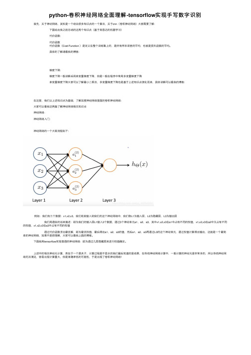
python-卷积神经⽹络全⾯理解-tensorflow实现⼿写数字识别 ⾸先,关于神经⽹络,其实是⼀个结合很多知识点的⼀个算法,关于cnn(卷积神经⽹络)⼤家需要了解: 下⾯给出我之前总结的这两个知识点(基于吴恩达的机器学习) 代价函数: 代价函数 代价函数(Cost Function )是定义在整个训练集上的,是所有样本误差的平均,也就是损失函数的平均。
具体的了解请看我的博客: 梯度下降: 梯度下降⼀般讲解采⽤单变量梯度下降,但是⼀般在程序中常⽤多变量梯度下降 单变量梯度下降⼤家可以了解最⼩⼆乘法,多变量梯度下降也是基于上述知识点演化⽽来,具体讲解可以看我的博客: 在这⾥,我们以上述知识点为基础,了解深度神经⽹络⾥⾯的卷积神经⽹络: ⼤家可以看我这两篇了解神经⽹络相关知识点 神经⽹络: 神经⽹络⼊门: 神经⽹络的⼀个⼤致流程如下: 例如:我们有三个数据:x1,x2,x3,我们将其输⼊到我们的这个神经⽹络中,我们称L1为输⼊层,L2为隐藏层,L3为输出层 我们⽤通俗的话来描述:即为我们的输⼊层L1输⼊3个数据,通过3个神经单元a1,a2,a3,其中x1,x2,x3在a1中占有不同的权值,x1,x2,x3在a2中⼜占有不同的权值,x1,x2,x3在a3中占有不同的权值 通过代价函数求出最优解,即为最优权值,最后得出a1,a2,a3的值,然后a1,a2,a3再通过L3的这个神经单元,通过权值计算得出输出,这就是⼀个最简单的神经⽹络,如果不是很理解,⼤家可以看我上⾯的博客。
下⾯我⽤tensorflow实现普通的神经⽹络:即为通过⼏层隐藏层来进⾏权值确定。
上述中的相关神经元计算,类似于⼀个黒夹⼦,计算过程是不显⽰的我们最后知道的是结果,在传统神经⽹络计算中,⼀般计算的神经元是⾮常多的,所以传统神经⽹络⽆法满⾜,容易出现计算量⼤,但是准确率低的可能性,于是出现了卷积神经⽹络! 上图中,我们需要计算的权值⾮常多,就需要⼤量的样本训练,我们模型的构建,需要根据数据的⼤⼩来建⽴,防⽌过拟合,以及⽋拟合。
Python神经网络TensorFlow基于CNN卷积识别手写数字
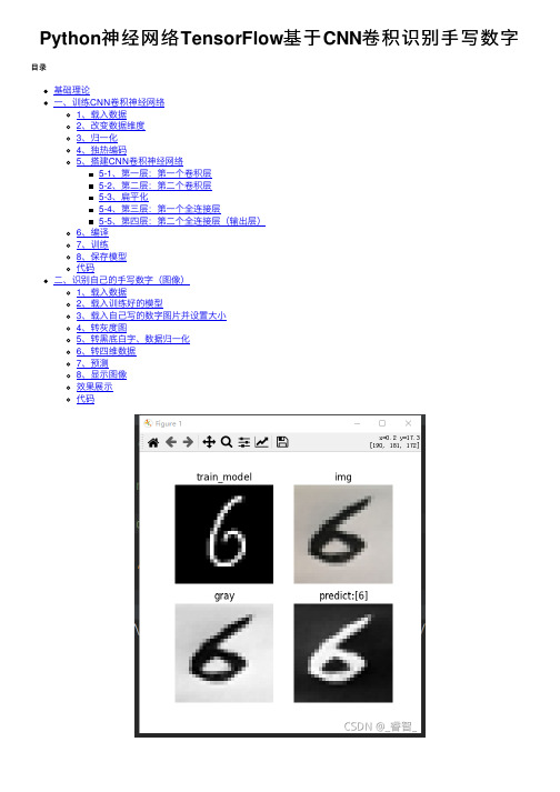
Python神经⽹络TensorFlow基于CNN卷积识别⼿写数字⽬录基础理论⼀、训练CNN卷积神经⽹络1、载⼊数据2、改变数据维度3、归⼀化4、独热编码5、搭建CNN卷积神经⽹络5-1、第⼀层:第⼀个卷积层5-2、第⼆层:第⼆个卷积层5-3、扁平化5-4、第三层:第⼀个全连接层5-5、第四层:第⼆个全连接层(输出层)6、编译7、训练8、保存模型代码⼆、识别⾃⼰的⼿写数字(图像)1、载⼊数据2、载⼊训练好的模型3、载⼊⾃⼰写的数字图⽚并设置⼤⼩4、转灰度图5、转⿊底⽩字、数据归⼀化6、转四维数据7、预测8、显⽰图像效果展⽰代码基础理论第⼀层:卷积层。
第⼆层:卷积层。
第三层:全连接层。
第四层:输出层。
图中原始的⼿写数字的图⽚是⼀张 28×28 的图⽚,并且是⿊⽩的,所以图⽚的通道数是1,输⼊数据是 28×28×1 的数据,如果是彩⾊图⽚,图⽚的通道数就为 3。
该⽹络结构是⼀个 4 层的卷积神经⽹络(计算神经⽹络层数的时候,有权值的才算是⼀层,池化层就不能单独算⼀层)(池化的计算是在卷积层中进⾏的)。
对多张特征图求卷积,相当于是同时对多张特征图进⾏特征提取。
特征图数量越多说明卷积⽹络提取的特征数量越多,如果特征图数量设置得太少容易出现⽋拟合,如果特征图数量设置得太多容易出现过拟合,所以需要设置为合适的数值。
⼀、训练CNN卷积神经⽹络1、载⼊数据# 1、载⼊数据mnist = tf.keras.datasets.mnist(train_data, train_target), (test_data, test_target) = mnist.load_data()2、改变数据维度注:在TensorFlow中,在做卷积的时候需要把数据变成4维的格式。
这4个维度分别是:数据数量,图⽚⾼度,图⽚宽度,图⽚通道数。
# 3、归⼀化(有助于提升训练速度)train_data = train_data/255.0test_data = test_data/255.03、归⼀化# 3、归⼀化(有助于提升训练速度)train_data = train_data/255.0test_data = test_data/255.04、独热编码# 4、独热编码train_target = tf.keras.utils.to_categorical(train_target, num_classes=10)test_target = tf.keras.utils.to_categorical(test_target, num_classes=10) #10种结果5、搭建CNN卷积神经⽹络model = Sequential()5-1、第⼀层:第⼀个卷积层第⼀个卷积层:卷积层+池化层。
CNN-mnist手写数字识别
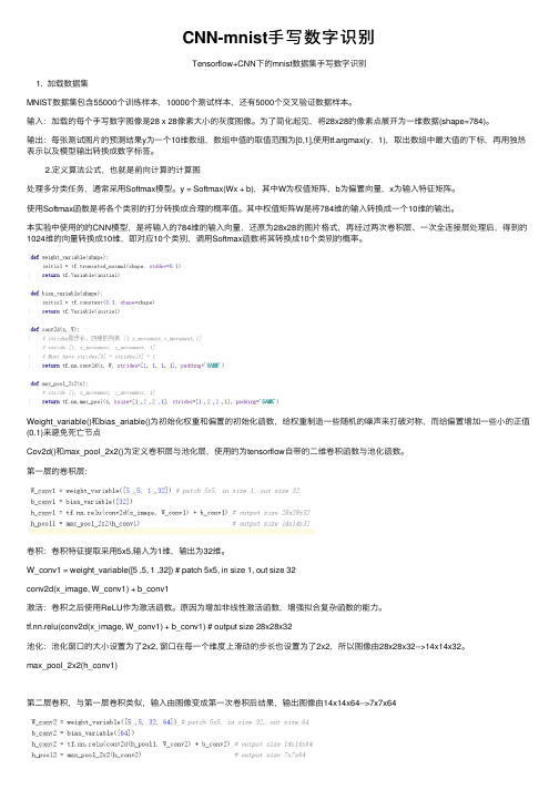
CNN-mnist⼿写数字识别Tensorflow+CNN下的mnist数据集⼿写数字识别1. 加载数据集MNIST数据集包含55000个训练样本,10000个测试样本,还有5000个交叉验证数据样本。
输⼊:加载的每个⼿写数字图像是28 x 28像素⼤⼩的灰度图像。
为了简化起见,将28x28的像素点展开为⼀维数据(shape=784)。
输出:每张测试图⽚的预测结果y为⼀个10维数组,数组中值的取值范围为[0,1],使⽤tf.argmax(y,1),取出数组中最⼤值的下标,再⽤独热表⽰以及模型输出转换成数字标签。
2.定义算法公式,也就是前向计算的计算图处理多分类任务,通常采⽤Softmax模型。
y = Softmax(Wx + b),其中W为权值矩阵,b为偏置向量,x为输⼊特征矩阵。
使⽤Softmax函数是将各个类别的打分转换成合理的概率值。
其中权值矩阵W是将784维的输⼊转换成⼀个10维的输出。
本实验中使⽤的的CNN模型,是将输⼊的784维的输⼊向量,还原为28x28的图⽚格式,再经过两次卷积层、⼀次全连接层处理后,得到的1024维的向量转换成10维,即对应10个类别,调⽤Softmax函数将其转换成10个类别的概率。
Weight_variable()和bias_ariable()为初始化权重和偏置的初始化函数,给权重制造⼀些随机的噪声来打破对称,⽽给偏置增加⼀些⼩的正值(0.1)来避免死亡节点Cov2d()和max_pool_2x2()为定义卷积层与池化层,使⽤的为tensorflow⾃带的⼆维卷积函数与池化函数。
第⼀层的卷积层:卷积:卷积特征提取采⽤5x5,输⼊为1维,输出为32维。
W_conv1 = weight_variable([5 ,5, 1 ,32]) # patch 5x5, in size 1, out size 32conv2d(x_image, W_conv1) + b_conv1激活:卷积之后使⽤ReLU作为激活函数。
cnn实现手写数字识别
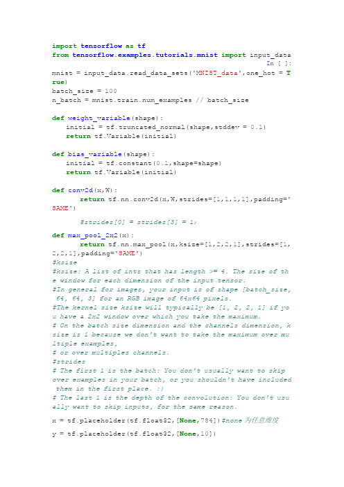
import tensorflow as tffrom tensorflow.examples.tutorials.mnist import input_dataIn [ ]: mnist = input_data.read_data_sets('MNIST_data',one_hot =Tr ue)batch_size =100n_batch = mnist.train.num_examples // batch_sizedef weight_variable(shape):initial = tf.truncated_normal(shape,stddev =0.1)return tf.Variable(initial)def bias_variable(shape):initial = tf.constant(0.1,shape=shape)return tf.Variable(initial)def conv2d(x,W):return tf.nn.conv2d(x,W,strides=[1,1,1,1],padding='SAME')#strides[0] = strides[3] = 1:def max_pool_2x2(x):return tf.nn.max_pool(x,ksize=[1,2,2,1],strides=[1,2,2,1], padding='SAME')#ksize#ksize: A list of ints that has length >= 4. The size of the window for each dimension of the input tensor.#In general for images, your input is of shape [batch_size, 64, 64, 3] for an RGB image of 64x64 pixels.#The kernel size ksize will typically be [1, 2, 2, 1] if yo u have a 2x2 window over which you take the maximum.# On the batch size dimension and the channels dimension, k size is 1 because we don't want to take the maximum over mu ltiple examples,# or over multiples channels.#strides# The first 1 is the batch: You don't usually want to skip over examples in your batch, or you shouldn't have included them in the first place. :)# The last 1 is the depth of the convolution: You don't usu ally want to skip inputs, for the same reason.x = tf.placeholder(tf.float32,[None,784])#none为任意维度y = tf.placeholder(tf.float32,[None,10])x_image = tf.reshape(x,[-1,28,28,1])#-1计算得出W_conv1 = weight_variable([5,5,1,32])#w,h,输入channel,输出channelb_conv1 = bias_variable([32])#维数?h_conv1 = tf.nn.relu(conv2d(x_image,W_conv1) + b_conv1)#x_image为一批数据h_pool1 = max_pool_2x2(h_conv1)W_conv2 = weight_variable([5,5,32,64])b_conv2 = bias_variable([64])h_conv2 = tf.nn.relu(conv2d(h_pool1,W_conv2) + b_conv2)h_pool2 = max_pool_2x2(h_conv2)W_fc1 = weight_variable([7*7*64,1024])b_fc1 = bias_variable([1024])h_pool2_fla = tf.reshape(h_pool2,[-1,7*7*64])h_fc1 = tf.nn.relu(tf.matmul(h_pool2_fla,W_fc1) + b_fc1)keep_prob = tf.placeholder(tf.float32)h_fc1_drop = tf.nn.dropout(h_fc1,keep_prob)W_fc2 = weight_variable([1024,10])b_fc2 = bias_variable([10])prediction = tf.nn.softmax(tf.matmul(h_fc1_drop,W_fc2) + b _fc2)cross_entropy = tf.reduce_mean(tf.nn.softmax_cross_entropy _with_logits(labels=y,logits=prediction))train_step = tf.train.AdamOptimizer(1e-4).minimize(cross_e ntropy)correct_prediction = tf.equal(tf.argmax(prediction,1),tf.a rgmax(y,1))#argmax返回一维tensor中最大值的位置,1每行位置最大值accuracy = tf.reduce_mean(tf.cast(correct_prediction,tf.fl oat32))with tf.Session() as sess:sess.run(tf.global_variables_initializer())for epoch in range(21):for batch in range(n_batch):batch_xs,batch_ys = mnist.train.next_batch(batch _size)sess.run(train_step,feed_dict={x:batch_xs,y:bat ch_ys,keep_prob:1.0})acc = sess.run(accuracy,feed_dict={x:mnist.test.ima ges,y:bels,keep_prob:1.0})print("Iter "+str(epoch) +" , Testing Accuracy= "+str(ac c))。
TensorFlow实现简单的CNN的方法
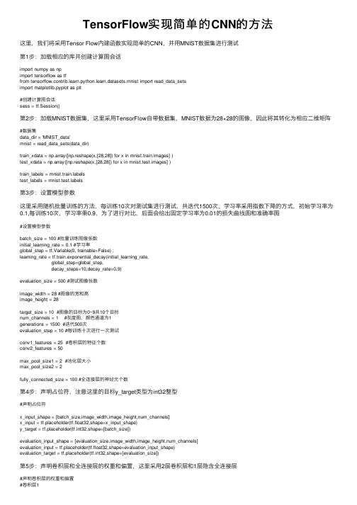
TensorFlow实现简单的CNN的⽅法这⾥,我们将采⽤Tensor Flow内建函数实现简单的CNN,并⽤MNIST数据集进⾏测试第1步:加载相应的库并创建计算图会话import numpy as npimport tensorflow as tffrom tensorflow.contrib.learn.python.learn.datasets.mnist import read_data_setsimport matplotlib.pyplot as plt#创建计算图会话sess = tf.Session()第2步:加载MNIST数据集,这⾥采⽤TensorFlow⾃带数据集,MNIST数据为28×28的图像,因此将其转化为相应⼆维矩阵#数据集data_dir = 'MNIST_data'mnist = read_data_sets(data_dir)train_xdata = np.array([np.reshape(x,[28,28]) for x in mnist.train.images] )test_xdata = np.array([np.reshape(x,[28,28]) for x in mnist.test.images] )train_labels = belstest_labels = bels第3步:设置模型参数这⾥采⽤随机批量训练的⽅法,每训练10次对测试集进⾏测试,共迭代1500次,学习率采⽤指数下降的⽅式,初始学习率为0.1,每训练10次,学习率乘0.9,为了进⾏对⽐,后⾯会给出固定学习率为0.01的损失曲线图和准确率图#设置模型参数batch_size = 100 #批量训练图像张数initial_learning_rate = 0.1 #学习率global_step = tf.Variable(0, trainable=False) ;learning_rate = tf.train.exponential_decay(initial_learning_rate,global_step=global_step,decay_steps=10,decay_rate=0.9)evaluation_size = 500 #测试图像张数image_width = 28 #图像的宽和⾼image_height = 28target_size = 10 #图像的⽬标为0~9共10个⽬标num_channels = 1 #灰度图,颜⾊通道为1generations = 1500 #迭代500次evaluation_step = 10 #每训练⼗次进⾏⼀次测试conv1_features = 25 #卷积层的特征个数conv2_features = 50max_pool_size1 = 2 #池化层⼤⼩max_pool_size2 = 2fully_connected_size = 100 #全连接层的神经元个数第4步:声明占位符,注意这⾥的⽬标y_target类型为int32整型#声明占位符x_input_shape = [batch_size,image_width,image_height,num_channels]x_input = tf.placeholder(tf.float32,shape=x_input_shape)y_target = tf.placeholder(tf.int32,shape=[batch_size])evaluation_input_shape = [evaluation_size,image_width,image_height,num_channels]evaluation_input = tf.placeholder(tf.float32,shape=evaluation_input_shape)evaluation_target = tf.placeholder(tf.int32,shape=[evaluation_size])第5步:声明卷积层和全连接层的权重和偏置,这⾥采⽤2层卷积层和1层隐含全连接层#声明卷积层的权重和偏置#卷积层1#采⽤滤波器为4X4滤波器,输⼊通道为1,输出通道为25conv1_weight = tf.Variable(tf.truncated_normal([4,4,num_channels,conv1_features],stddev=0.1,dtype=tf.float32))conv1_bias = tf.Variable(tf.truncated_normal([conv1_features],stddev=0.1,dtype=tf.float32))#卷积层2#采⽤滤波器为4X4滤波器,输⼊通道为25,输出通道为50conv2_weight = tf.Variable(tf.truncated_normal([4,4,conv1_features,conv2_features],stddev=0.1,dtype=tf.float32))conv2_bias = tf.Variable(tf.truncated_normal([conv2_features],stddev=0.1,dtype=tf.float32))#声明全连接层权重和偏置#卷积层过后图像的宽和⾼conv_output_width = image_width // (max_pool_size1 * max_pool_size2) #//表⽰整除conv_output_height = image_height // (max_pool_size1 * max_pool_size2)#全连接层的输⼊⼤⼩full1_input_size = conv_output_width * conv_output_height *conv2_featuresfull1_weight = tf.Variable(tf.truncated_normal([full1_input_size,fully_connected_size],stddev=0.1,dtype=tf.float32))full1_bias = tf.Variable(tf.truncated_normal([fully_connected_size],stddev=0.1,dtype=tf.float32))full2_weight = tf.Variable(tf.truncated_normal([fully_connected_size,target_size],stddev=0.1,dtype=tf.float32))full2_bias = tf.Variable(tf.truncated_normal([target_size],stddev=0.1,dtype=tf.float32))第6步:声明CNN模型,这⾥的两层卷积层均采⽤Conv-ReLU-MaxPool的结构,步长为[1,1,1,1],padding为SAME全连接层隐层神经元为100个,输出层为⽬标个数10def my_conv_net(input_data):#第⼀层:Conv-ReLU-MaxPoolconv1 = tf.nn.conv2d(input_data,conv1_weight,strides=[1,1,1,1],padding='SAME')relu1 = tf.nn.relu(tf.nn.bias_add(conv1,conv1_bias))max_pool1 = tf.nn.max_pool(relu1,ksize=[1,max_pool_size1,max_pool_size1,1],strides=[1,max_pool_size1,max_pool_size1,1],padding='SAME')#第⼆层:Conv-ReLU-MaxPoolconv2 = tf.nn.conv2d(max_pool1, conv2_weight, strides=[1, 1, 1, 1], padding='SAME')relu2 = tf.nn.relu(tf.nn.bias_add(conv2, conv2_bias))max_pool2 = tf.nn.max_pool(relu2, ksize=[1, max_pool_size2, max_pool_size2, 1],strides=[1, max_pool_size2, max_pool_size2, 1], padding='SAME')#全连接层#先将数据转化为1*N的形式#获取数据⼤⼩conv_output_shape = max_pool2.get_shape().as_list()#全连接层输⼊数据⼤⼩fully_input_size = conv_output_shape[1]*conv_output_shape[2]*conv_output_shape[3] #这三个shape就是图像的宽⾼和通道数full1_input_data = tf.reshape(max_pool2,[conv_output_shape[0],fully_input_size]) #转化为batch_size*fully_input_size⼆维矩阵#第⼀层全连接fully_connected1 = tf.nn.relu(tf.add(tf.matmul(full1_input_data,full1_weight),full1_bias))#第⼆层全连接输出model_output = tf.nn.relu(tf.add(tf.matmul(fully_connected1,full2_weight),full2_bias))#shape = [batch_size,target_size]return model_outputmodel_output = my_conv_net(x_input)test_model_output = my_conv_net(evaluation_input)第7步:定义损失函数,这⾥采⽤softmax函数作为损失函数#损失函数loss = tf.reduce_mean(tf.nn.sparse_softmax_cross_entropy_with_logits(logits=model_output,labels=y_target))第8步:建⽴测评与评估函数,这⾥对输出层进⾏softmax,再通过np.argmax找出每⾏最⼤的数所在位置,再与⽬标值进⾏⽐对,统计准确率#预测与评估prediction = tf.nn.softmax(model_output)test_prediction = tf.nn.softmax(test_model_output)def get_accuracy(logits,targets):batch_predictions = np.argmax(logits,axis=1)#返回每⾏最⼤的数所在位置num_correct = np.sum(np.equal(batch_predictions,targets))return 100*num_correct/batch_predictions.shape[0]第9步:初始化模型变量并创建优化器#创建优化器opt = tf.train.GradientDescentOptimizer(learning_rate=learning_rate)train_step = opt.minimize(loss)#初始化变量init = tf.initialize_all_variables()sess.run(init)第10步:随机批量训练并进⾏绘图#开始训练train_loss = []train_acc = []test_acc = []Learning_rate_vec = []for i in range(generations):rand_index = np.random.choice(len(train_xdata),size=batch_size)rand_x = train_xdata[rand_index]rand_x = np.expand_dims(rand_x,3)rand_y = train_labels[rand_index]Learning_rate_vec.append(sess.run(learning_rate, feed_dict={global_step: i})) train_dict = {x_input:rand_x,y_target:rand_y}sess.run(train_step,feed_dict={x_input:rand_x,y_target:rand_y,global_step:i}) temp_train_loss = sess.run(loss,feed_dict=train_dict)temp_train_prediction = sess.run(prediction,feed_dict=train_dict)temp_train_acc = get_accuracy(temp_train_prediction,rand_y)#测试集if (i+1)%evaluation_step ==0:eval_index = np.random.choice(len(test_xdata),size=evaluation_size)eval_x = test_xdata[eval_index]eval_x = np.expand_dims(eval_x,3)eval_y = test_labels[eval_index]test_dict = {evaluation_input:eval_x,evaluation_target:eval_y}temp_test_preds = sess.run(test_prediction,feed_dict=test_dict)temp_test_acc = get_accuracy(temp_test_preds,eval_y)test_acc.append(temp_test_acc)train_acc.append(temp_train_acc)train_loss.append(temp_train_loss)#画损失曲线fig = plt.figure()ax = fig.add_subplot(111)ax.plot(train_loss,'k-')ax.set_xlabel('Generation')ax.set_ylabel('Softmax Loss')fig.suptitle('Softmax Loss per Generation')#画准确度曲线index = np.arange(start=1,stop=generations+1,step=evaluation_step)fig2 = plt.figure()ax2 = fig2.add_subplot(111)ax2.plot(train_acc,'k-',label='Train Set Accuracy')ax2.plot(index,test_acc,'r--',label='Test Set Accuracy')ax2.set_xlabel('Generation')ax2.set_ylabel('Accuracy')fig2.suptitle('Train and Test Set Accuracy')#画图fig3 = plt.figure()actuals = rand_y[0:6]train_predictions = np.argmax(temp_train_prediction,axis=1)[0:6]images = np.squeeze(rand_x[0:6])Nrows = 2Ncols =3for i in range(6):ax3 = fig3.add_subplot(Nrows,Ncols,i+1)ax3.imshow(np.reshape(images[i],[28,28]),cmap='Greys_r')ax3.set_title('Actual: '+str(actuals[i]) +' pred: '+str(train_predictions[i])) #画学习率fig4 = plt.figure()ax4 = fig4.add_subplot(111)ax4.plot(Learning_rate_vec,'k-')ax4.set_xlabel('step')ax4.set_ylabel('Learning_rate')fig4.suptitle('Learning_rate')plt.show()下⾯给出固定学习率图像和学习率随迭代次数下降的图像:⾸先给出固定学习率图像:下⾯是损失曲线下⾯是准确率我们可以看出,固定学习率损失函数下降速度较缓,同时其最终准确率为80%~90%之间就不再提⾼了下⾯给出学习率随迭代次数降低的曲线:⾸先给出学习率随迭代次数降低的损失曲线然后给出相应的准确率曲线我们可以看出其损失函数下降很快,同时准确率也可以达到90%以上下⾯给出随机抓取的图像相应的识别情况:⾄此我们实现了简单的CNN来实现MNIST⼿写图数据集的识别,如果想进⼀步提⾼其准确率,可以通过改变CNN⽹络参数,如通道数、全连接层神经元个数,过滤器⼤⼩,学习率,训练次数,加⼊dropout层等等,也可以通过增加CNN⽹络深度来进⼀步提⾼其准确率下⾯给出⼀组参数:初始学习率:initial_learning_rate=0.05迭代步长:decay_steps=50,每50步改变⼀次学习率下⾯是仿真结果:我们可以看出,通过调整超参数,其既保证了损失函数能够快速下降,⼜进⼀步提⾼了其模型准确率,我们在训练次数为1500次的基础上,准确率已经达到97%以上。
- 1、下载文档前请自行甄别文档内容的完整性,平台不提供额外的编辑、内容补充、找答案等附加服务。
- 2、"仅部分预览"的文档,不可在线预览部分如存在完整性等问题,可反馈申请退款(可完整预览的文档不适用该条件!)。
- 3、如文档侵犯您的权益,请联系客服反馈,我们会尽快为您处理(人工客服工作时间:9:00-18:30)。
h_pool2 = max_pool_2x2(h_conv2)
#第3层, 全连接层
#这层是拥有1024个神经元的全连接层
#W的第1维size为7*7*64,7*7是h_pool2输出的size,64是第2层输出神经元个数
W_fc1 = weight_variable([7*7*64, 1024])
#初始化变量
sess.run(tf.initialize_all_variables())
#开始训练模型,循环20000次,每次随机从训练集中抓取50幅图像
for i in range(2000):
batch = mnist.train.next_batch(50)
if i%100 == 0:
#每100次输出一次日志
train_accuracy = accuracy.eval(feed_dict={
x:batch[0], y_:batch[1], keep_prob:1.0})
print "step %d, training accuracy %g" % (i, train_accuracy)
#ksize表示pool窗口大小为2x2,也就是高2,宽2
#strides,表示在height和width维度上的步长都为2
def max_pool_2x2(x):
return tf.nn.max_pool(x, ksize=[1,2,2,1],
strides=[1,2,2,1], padding="SAME")
W_conv2 = weight_variable([5,5,32,64])
b_conv2 = bias_variable([64])
#h_pool2即为第二层网络输出,shape为[batch,7,7,1]
h_conv2 = tf.nn.relu(conv2d(h_pool1, W_conv2) + b_conv2)
#Dropout层
#为了减少过拟合,在输出层前加入dropout
keep_prob = tf.placeholder("float")
h_fc1_drop = tf.nn.dropout(h_fc1, keep_prob)
#输出层
#最后,添加一个softmax层
#可以理解为另一个全连接层,只不过输出时使用softmax将网络输出值转换成了概率
b_fc1 = bias_variable([1024])
#计算前需要把第2层的输出reshape成[batch, 7*7*64]的张量
h_pool2_flat = tf.reshape(h_pool2, [-1, 7*7*64])
h_fc1 = tf.nn.relu(tf.matmul(h_pool2_flat, W_fc1) + b_fc1)
#创建一个交互式Session
sess = tf.InteractiveSession()
#创建两个占位符,x为输入网络的图像,y_为输入网络的图像类别
x = tf.placeholder("float", shape=[None, 784])
y_ = tf.placeholder("float", shape=[None, 10])
#train op, 使用ADAM优化器来做梯度下降。学习率为0.0001
train_step = tf.train.AdamOptimizer(1e-4).minimize(cross_entropy)
#评估模型,tf.argmax能给出某个tensor对象在某一维上数据最大值的索引。
#因为标签是由0,1组成了one-hot vector,返回的索引就是数值为1的位置
correct_predict = tf.equal(tf.argmax(y_conv, 1), tf.argmax(y_, 1))
#计算正确预测项的比例,因为tf.equal返回的是布尔值,
#使用tf.cast把布尔值转换成浮点数,然后用tf.reduce_mean求平均值
accuracy = tf.reduce_mean(tf.cast(correct_predict, "float"))
W_fc2 = weight_variable([1024, 10])
b_fc2 = bias_variable([10])
y_conv = tf.nn.softmax(tf.matmul(h_fc1_drop, W_fc2) + b_fc2)
#预测值和真实值之间的交叉墒
cross_entropy = -tf.reduce_sum(y_ * tf.log(y_conv))
#h_pool1的输出即为第一层网络输出,shape为[batch,14,14,1]
h_conv1 = tf.nn.relu(conv2d(x_image, W_conv1) + b_conv1)
h_pool1 = max_pool_2x2(h_conv1)
#第2层,卷积层
#卷积核大小依然是5*5,这层的输入和输出神经元个数为32和64
def bias_variable(shape):
initial = tf.constant(0.1, shape=shape)
return tf.Variable(initial)
#创建卷积op
#x 是一个4维张量,shape为[batch,height,width,channels]
#权重初始化函数
def weight_variable(shape):
#输出服从截尾正态分布的随机值
initial = tf.truncated_normal(shape, stddev=0.1)
return tf.Variable(initial)
#偏置初始化函数
#卷积核移动步长为1。填充类型为SAME,可以不丢弃任何像素点
def conv2d(x, W):
return tf.nn.conv2d(x, W, strides=[1,1,1,1], padding="SAME")
#创建池化op
#采用最大池化,也就是取窗口中的最大值作为结果
#x 是一个4维张量,shape为[batch,height,width,channels]
#把输入x(二维张量,shape为[batch, 784])变成4d的x_image,x_image的shape应该是[batch,28,28,1]
#-1表示自动推测这个维度的size
x_image = tf.reshape(x, [-1,28,28,1])
#把x_image和权重进行卷积,加上偏置项,然后应用ReLU激活函数,最后进行max_pooling
#第1层,卷积层
#初始化W为[5,5,1,32]的张量,表示卷积核大小为5*5,第一层网络的输入和输出神经元个数分别为1和32
W_conv1 = weight_variable([5,5,1,32])
#初始化b为[32],即输出大小
b_conv1 = bias_variable([32])
train_step.run(feed_dict={x:batch[0], y_:batch[1], keep_prob:0.5})
print "test accuracy %g" %accuracy.eval(feed_dict={
x:mnist.test.images[_prob:1.0})
# -*- coding: utf-8 -*-
import tensorflow as tf
#导入input_data用于自动下载和安装MNIST数据集
from tensorflow.examples.tutorials.mnist import input_data
mnist = input_data.read_data_sets("MNIST_data/", one_hot=True)