统计学重点整理CH7 Distributions of the Sample Mean and Sample Proportion and Sampling Techniques
戴维商务统计学第7版英文版教学指南CH07_Levine7e_ISM
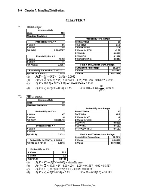
240 Chapter 7: Sampling DistributionsCHAPTER 77.1 PHstat output:Common DataMean 100Standard Deviation 2Probability for a RangeProbability for X <= From X Value 95 X Value 95To X Value 97.5 Z Value -2.5Z Value for 95 -2.5 P(X<=95) 0.0062097Z Value for 97.5 -1.25P(X<=95) 0.0062 Probability for X > P(X<=97.5) 0.1056 X Value 102.2P(95<=X<=97.5) 0.0994 Z Value 1.1P(X>102.2) 0.1357Find X and Z Given Cum. Pctage.Cumulative Percentage 35.00%Z Value -0.38532X Value 99.22936(b) P(95 < X < 97.5) = P(– 2.50 < Z < – 1.25) = 0.1056 – 0.0062 = 0.0994(c) P(X > 102.2) = P(Z > 1.10) = 1.0 – 0.8643 = 0.1357(d) P(X > A) = P(Z > – 0.39) = 0.65X = 100 – 0.39(1025) = 99.227.2 PHStat output:Common DataMean 50Standard Deviation 0.5Probability for a RangeProbability for X <= From X Value 47 X Value 47To X Value 49.5 Z Value -6Z Value for 47 -6 P(X<=47) 9.866E-10Z Value for 49.5 -1P(X<=47) 0.0000 Probability for X > P(X<=49.5) 0.1587 X Value 51.5P(47<=X<=49.5) 0.1587 Z Value 3P(X>51.5) 0.0013Find X and Z Given Cum. Pctage.Cumulative Percentage 65.00% Probability for X<47 or X >51.5 Z Value 0.38532 P(X<47 or X >51.5) 0.0013X Value 50.19266(b) P(47 < X < 49.5) = P(– 6.00 < Z < – 1.00) = 0.1587 – 0.00 = 0.1587(c) P(X > 51.1) = P(Z > 2.20) = 1.0 – 0.9861 = 0.0139(d) P(X > A) = P(Z > 0.39) = 0.35 X = 50 + 0.39(0.5) = 50.195Solutions to End-of-Section and Chapter Review Problems 241 7.3 (a) For samples of 25 customer receipts for a supermarket for a year, the samplingdistribution of sample means is the distribution of means from all possible samples of 25customer receipts for a supermarket for that year.(b) For samples of 25 insurance payouts in a particular geographical area in a year, thesampling distribution of sample means is the distribution of means from all possiblesamples of 25 insurance payouts in that particular geographical area in that year.(c) For samples of 25 Call Center logs of inbound calls tracking handling time for a creditcard company during the year, the sampling distribution of sample means is thedistribution of means from all possible samples of 25 Call Center logs of inbound callstracking handling time for a credit card company during that year.7.4 (a) Sampling Distribution of the Mean for n = 2 (without replacement)iX1 1, 31X = 22 1, 62X = 3.53 1, 73X = 44 1, 94X = 55 1, 105X = 5.56 3, 66X = 4.57 3, 77X = 58 3, 98X = 69 3, 109X = 6.510 6, 710X = 6.511 6, 911X = 7.512 6, 1012X = 813 7, 913X = 814 7, 1014X = 8.515 9, 1015X = 9.5(a) Mean of All Possible Sample Means: Mean of All Population Elements:μX =9015=6136791066μ+++++==Both means are equal to 6. This property is called unbiasedness.242 Chapter 7: Sampling Distributions7.4 (b) Sampling Distribution of the Mean for n = 3 (without replacement) cont.X1 1, 3, 61X = 3 1/32 1, 3, 72X = 3 2/33 1, 3, 93X = 4 1/34 1, 3, 104X = 4 2/35 1, 6, 75X = 4 2/36 1, 6, 96X = 5 1/37 1, 6, 107X = 5 2/38 3, 6, 78X = 5 1/39 3, 6, 99X = 610 3, 6, 1010X = 6 1/311 6, 7, 911X = 7 1/312 6, 7, 1012X = 7 2/313 6, 9, 1013X = 8 1/314 7, 9, 1014X = 8 2/315 1, 7, 915X = 5 2/316 1, 7, 1016X = 617 1, 9, 1017X = 6 2/318 3, 7, 918X = 6 1/319 3, 7, 1019X = 6 2/320 3, 9, 1020X = 7 1/3μX =12020=6This is equal toμ, the population mean.(c) The distribution for n = 3 has less variability. The larger sample size has resulted in samplemeans being closer toμ.(d) (a) Sampling Distribution of the Mean for n = 2 (with replacement)Solutions to End-of-Section and Chapter Review Problems 243 7.4cont.XiX1X = 22 1, 32X = 3.53 1, 63X = 44 1, 74X = 55 1, 95X = 5.56 1, 106X = 27 3, 17X = 38 3, 38X = 4.59 3, 69X = 510 3, 710X = 611 3, 911X = 6.512 3, 1012X = 3.513 6, 113X = 4.514 6, 314X = 615 6, 615X = 6.516 6, 716X = 7.517 6, 917X = 818 6, 1018X= 419 7, 119X = 520 7, 320X = 6.521 7, 621X = 722 7, 722X = 823 7, 923X = 8.524 7, 1024X = 525 9, 125X = 626 9, 326X = 7.527 9, 627X = 828 9, 728X = 929 9, 929X = 9.530 9, 1030X = 5.531 10, 131X = 6.532 10, 332X = 833 10, 633X = 8.534 10, 734X = 9.535 10, 935X = 1036 10, 1036244 Chapter 7: Sampling Distributions 7.4 (d) (a) Mean of All Possible Mean of All cont. Sample Means: Population Elements:216636X μ== μ=1+3+6+7+7+126=6Both means are equal to 6. This property is called unbiasedness. (b) Repeat the same process for the sampling distribution of the mean for n = 3 (withreplacement). There will be 36216= different samples.6X μ= This is equal to μ, the population mean.(c) The distribution for n = 3 has less variability. The larger sample size has resulted inmore sample means being close to μ. 7.5(a)Because the population diameter of tennis balls is approximately normally distributed, the sampling distribution of samples of 9 will also be approximately normal with a mean ofX μμ== 2.63 and X σ== 0.01.(b)X(c)Upper bound: X = 2.6384Solutions to End-of-Section and Chapter Review Problems 2457.6 (a)When n = 4 , the shape of the sampling distribution of X should closely resemble the shape of the distribution of the population from which the sample is selected. Because the mean is larger than the median, the distribution of the sales price of new houses is skewed to the right, and so is the sampling distribution of X although it will be less skewed than the population.(b)If you select samples of n = 100, the shape of the sampling distribution of the sample mean will be very close to a normal distribution with a mean of $322,100 and a standarddeviation of X σ== $9,000.(c) X σ =900010090000==nσ(d)7.7 (a) X σ1==246 Chapter 7: Sampling Distributions 7.7 (b) PHStat output: cont.(c) X σ0.5==(d) With the sample size increasing from n = 25 to n = 100, more sample means will becloser to the distribution mean. The standard error of the sampling distribution of size 100 is much smaller than that of size 25, so the likelihood that the sample mean will fall within ±0.5 minutes of the mean is much higher for samples of size 100 (probability = 0.6827) than for samples of size 25 (probability = 0. 3829).7.8(b) P (X < A ) = P (Z < 1.0364) = 0.85 X = 27 + 1.0364 (1) = 28.0364(c) To be able to use the standard normal distribution as an approximation for the area underthe curve, we must assume that the population is symmetrically distributed such that the central limit theorem will likely hold for samples of n = 16.(d)X = 27 + 1.0364 (0.5) = 27.5182Solutions to End-of-Section and Chapter Review Problems 2477.9 (a)p = 48/64 = 0.75(b)p σ =64)30.0(70.0 = 0.05737.10 (a)p = 20/50 = 0.40(b)p σ= 7.11 (a) p = 14/40 = 0.35(b)p σ =40)70.0(30.0 = 0.07257.12 (a) 0.501p μπ==, 0.05p σ===Partial PHstat output:Probability for X > X Value 0.55Z Value 0.98P(X>0.55) 0.1635P (p > 0.55) = P (Z > 0.98) = 1 – 0.8365 = 0.1635(b) 0.60p μπ==, 0.04899p σ===Partial PHstat output:Probability for X > X Value 0.55Z Value -1.020621P(X>0.55) 0.8463P (p > 0.55) = P (Z > – 1.021) = 1 – 0.1539 = 0.8461(c) 0.49p μπ==, 0.05p σ===Partial PHstat output:Probability for X > X Value 0.55Z Value 1.2002401P(X>0.55) 0.1150P (p > 0.55) = P (Z > 1.20) = 1 – 0.8849 = 0.1151(d) Increasing the sample size by a factor of 4 decreases the standard error by a factor of 2.248 Chapter 7: Sampling Distributions7.12 (d) (a) Partial PHstat output:cont.Probability for X >X Value 0.55Z Value 1.9600039P(X>0.55) 0.0250P(p > 0.55) = P (Z > 1.96) = 1 – 0.9750 = 0.0250(b) Partial PHstat output:Probability for X >X Value 0.55Z Value -2.041241P(X>0.55) 0.9794P(p > 0.55) = P (Z > – 2.04) = 1 – 0.0207 = 0.9793(c) Partial PHstat output:Probability for X >X Value 0.55Z Value 2.4004801P(X>0.55) 0.0082P(p > 0.55) = P (Z > 2.40) = 1 – 0.9918 = 0.0082If the sample size is increased to 400, the probably in (a), (b) and (c) is smaller,larger, and smaller, respectively because the standard error of the samplingdistribution of the sample proportion becomes smaller and, hence, the samplingdistribution is more concentrated around the true population proportion.7.13 (a) Partial PHstat output:Probability for a RangeFrom X Value 0.5To X Value 0.6Z Value for 0.5 0Z Value for 0.6 2.828427P(X<=0.5) 0.5000P(X<=0.6) 0.9977P(0.5<=X<=0.6) 0.4977P(0.50 < p < 0.60) = P(0 < Z < 2.83) = 0.4977(b) Partial PHstat output:Find X and Z Given Cum. Pctage.Cumulative Percentage 95.00%Z Value 1.644854X Value 0.558154P(– 1.645 < Z < 1.645) = 0.90p = .50 – 1.645(0.0354) = 0.4418 p = .50 + 1.645(0.0354) = 0.5582(c) Partial PHstat output:Probability for X >X Value 0.65Z Value 4.2426407P(X>0.65) 0.0000P(p > 0.65) = P (Z > 4.24) = virtually zeroSolutions to End-of-Section and Chapter Review Problems 2497.13 (d)Partial PHstat output:cont.Probability for X > X Value 0.6Z Value 2.8284271P(X>0.6) 0.0023If n = 200, P (p > 0.60) = P (Z > 2.83) = 1.0 – 0.9977 = 0.0023Probability for X > X Value 0.55Z Value 3.1622777P(X>0.55) 0.00078If n = 1000, P (p > 0.55) = P (Z > 3.16) = 1.0 – 0.99921 = 0.00079More than 60% correct in a sample of 200 is more likely than more than 55% correct in asample of 1000.7.14 (a) ==πμp 0.80, ()np ππσ−=1(b)(c)250 Chapter 7: Sampling Distributions 7.14 (d) ==πμp 0.80, ()n p ππσ−=1cont.(b)(c)7.15 (a) ==πμp 0.57, ()np ππσ−=1 = 0.0495(b)Solutions to End-of-Section and Chapter Review Problems 2517.15 (c)(d) ==πμp 0.57, ()np ππσ−=1 = 0.0248(a)(b)(c)7.16 (a)population proportion and, hence,π=0.15. Also the sampling distribution of the sample proportion will be close to a normal distribution according to the central limit theorem.252 Chapter 7: Sampling Distributions7.16p μπ==0.15,p σ=== 0.0252cont. P (0.12 < p < 0.18) = P (-1.1882< Z < 1.1882) = 0.7652A = 0.1085B = 0.1915A = 0.1005B = 0.1995 7.17 (a) p μπ==0.49, p σ=== 0.0500A = 0.4078B = 0.5722Solutions to End-of-Section and Chapter Review Problems 2537.17 (c)Partial PHStat output:cont.A = 0.3920B = 0.5880(d) (a) p μπ==0.49, p σ=== 0.02500.6007A = 0.4489B = 0.5311 (c)A = 0.4410B = 0.5390254 Chapter 7: Sampling Distributions 7.18 (a) ==πμp 0.36, ()n p ππσ−=1= 0.0480(b)= 0.0240(c)Increasing the sample size by a factor of 4 decreases the standard error by a factor of . The sampling distribution of the proportion becomes more concentrated around the true proportion of 0.36 and, hence, the probability in (b) becomes smaller than that in (a).7.19 Because the average of all the possible sample means of size n is equal to the population mean.7.20 The variation of the sample means becomes smaller as larger sample sizes are taken. This is dueto the fact that an extreme observation will have a smaller effect on the mean in a larger sample than in a small sample. Thus, the sample means will tend to be closer to the population mean as the sample size increases.7.21 As larger sample sizes are taken, the effect of extreme values on the sample mean becomessmaller and smaller. With large enough samples, even though the population is not normally distributed, the sampling distribution of the mean will be approximately normally distributed.7.22 The population distribution is the distribution of a particular variable of interest, while thesampling distribution represents the distribution of a statistic.7.23 When the items of interest and the items not of interest are at least 5, the normal distribution canbe used to approximate the binomial distribution.Solutions to End-of-Section and Chapter Review Problems 2557.24 0.753X μ=5004.0==nX σσ = 0.0008PHStat output:Common DataMean 0.753 Standard Deviation 0.0008Probability for a RangeProbability for X <=From X Value 0.75 X Value 0.74 To X Value 0.753 Z Value -16.25 Z Value for 0.75 -3.75 P(X<=0.74) 1.117E-59 Z Value for 0.753 0P(X<=0.75) 0.0001 Probability for X >P(X<=0.753) 0.5000 X Value 0.76 P(0.75<=X<=0.753) 0.4999 Z Value 8.75P(X>0.76) 0.0000 Find X and Z Given Cum. Pctage.Cumulative Percentage 7.00% Probability for X<0.74 or X >0.76 Z Value -1.475791 P(X<0.74 or X >0.76) 0.0000X Value 0.751819Probability for a Range From X Value 0.74 To X Value 0.75 Z Value for 0.74 -16.25 Z Value for 0.75 -3.75 P(X<=0.74) 0.0000 P(X<=0.75) 0.0001 P(0.74<=X<=0.75) 0.00009(a) P (0.75 < X < 0.753) = P (– 3.75 < Z < 0) = 0.5 – 0.00009 = 0.4999 (b) P (0.74 < X < 0.75) = P (– 16.25 < Z < – 3.75) = 0.00009 (c) P (X > 0.76) = P (Z > 8.75) = virtually zero (d) P (X < 0.74) = P (Z < – 16.25) = virtually zero (e) P (X < A ) = P (Z < – 1.48) = 0.07 X = 0.753 – 1.48(0.0008) = 0.7518256 Chapter 7: Sampling Distributions 7.25 2.0X μ=505.0==nX σσ = 0.01PHStat output:Common DataMean 2 Standard Deviation 0.01Probability for a RangeProbability for X <= From X Value 1.99X Value 1.98 To X Value 2Z Value -2 Z Value for 1.99 -1P(X<=1.98) 0.0227501 Z Value for 2 0P(X<=1.99) 0.1587Probability for X >P(X<=2) 0.5000X Value 2.01 P(1.99<=X<=2) 0.3413Z Value 1P(X>2.01) 0.1587 Find X and Z Given Cum. Pctage.Cumulative Percentage 1.00%Probability for X<1.98 or X>2.01Z Value-2.326348P(X<1.98 or X >2.01) 0.1814 X Value 1.976737Find X and Z Given Cum. Pctage.Cumulative Percentage 99.50% Z Value 2.575829X Value2.025758(a) P (1.99 < X < 2.00) = P (– 1.00 < Z < 0) = 0.5 – 0.1587 = 0.3413 (b) P (X < 1.98) = P (Z < – 2.00) = 0.0228(c) P (X > 2.01) = P (Z > 1.00) = 1.0 – 0.8413 = 0.1587(d) P (X > A ) = P ( Z > – 2.33) = 0.99 A= 2.00 – 2.33(0.01) = 1.9767 (e) P (A < X < B ) = P (– 2.58 < Z < 2.58) = 0.99A = 2.00 – 2.58(0.01) = 1.9742B = 2.00 + 2.58(0.01) = 2.0258Solutions to End-of-Section and Chapter Review Problems 2577.26 4.7X μ=0.400.085X σ===PHstat output:Common DataMean 4.7 Standard Deviation 0.08Probability for X >Find X and Z Given Cum. Pctage. X Value 4.6 Cumulative Percentage 23.00% Z Value -1.25 Z Value -0.738847 P(X>4.6) 0.8944 X Value 4.640892Find X and Z Given Cum. Pctage. Find X and Z Given Cum. Pctage. Cumulative Percentage 15.00% Cumulative Percentage 85.00% Z Value -1.036433 Z Value 1.036433 X Value 4.6170853X Value 4.782915(a) P (4.60 < X ) = P (– 1.25 < Z ) = 1 – 0.1056 = 0.8944 (b) P (A < X < B ) = P (– 1.04 < Z < 1.04) = 0.70A = 4.70 – 1.04(0.08) = 4.6168 ounces X = 4.70 + 1.04(0.08) = 4.7832 ounces(c) P (X > A ) = P (Z > – 0.74) = 0.77A = 4.70 – 0.74(0.08) = 4.6408 7.27X μ=5.00.400.085X σ===(a)Partial PHStat output:Probability for X > X Value 4.6 Z Value -5 P(X>4.6)1.0000P (4.60 < X ) = P (– 5 < Z ) = essentially 1.0 (b) Partial PHStat output:Find X and Z Given Cum. Pctage. Cumulative Percentage 15.00% Z Value -1.036433 X Value 4.917085A = 5.0 – 1.0364(0.08) = 4.9171 ounces X = 5.0 + 1.0364(0.08) = 5.0829 ounces258 Chapter 7: Sampling Distributions7.27 (c) Partial PHStat output: cont.Find X and Z Given Cum. Pctage. Cumulative Percentage 23.00% Z Value -0.738847 X Value4.940892P (X > A ) = P (Z > – 0.7388) = 0.77 A = 5.0 – 0.7388(0.08) = 4.94097.28 μμ=X = 15.23, X σ=(a)(b)(c)7.29 (a) μ=3.17 σ = 10Solutions to End-of-Section and Chapter Review Problems 2597.29 (b)Partial PHStat output:cont.(c)(d) μμ=X= 3.17, X σ== 5(e)(f)(g)Since the sample mean of returns of a sample of stocks is distributed closer to the population mean than the return of a single stock, the probabilities in (a) and (b) are higher than those in (d) and (e) while the probability in (c) is lower than that in (f).。
Chapter 7 Distribution of Sample Means

Chapter 8 & (part) Chapter 12: Distribution of SampleMeansWe’ve been examining Z-scores & the probability of obtaining individual scores within a normal distributionBut inferential statistics involve samples of more than 1To transition into inferential statistics, it is important that we understand how probability relates to sample means, not just individual scores Inferential statistics: sample infer something about populationOften not possible to measure everyone in a populationSamples are convenient representations of themIf you take multiple samples of the same size from a population, they are likely to give different resultsSamples vary!Quite likely that a particular sample won’t reflect the population exactly Discrepancy b/n sample & population = sampling errorThe term “sampling error” does not mean a sampling mistake – rather it indicates that means drawn from multiple samples taken from apopulation will vary from each other due to random chance andtherefore may deviate from the population meanWhat is a distribution of Sample Means (Sampling Distribution of the Mean)?A distribution of sample means (X); a “distribution of a statistic [in this casea sample mean] over repeated sampling from a specified population”Based on all possible random samples of size n, from a populationCan inform us of the degree of sample-to-sample variability we should expect due to chanceSuppose we have a population: 6 7 8 9 μ = 7.5 Let’s take all possible samples of size n = 2 from this population:1. 6 6 X= 6.0 7. 7 8 X= 7.513. 9 6 X= 7.52. 6 7 = 6.5 8. 7 9 = 8.0 14. 9 7 = 8.03. 6 8 X= 7.0 9. 8 6 X= 7.0 15. 9 8 X= 8.54. 6 9 X= 7.510. 8 7 X= 7.516. 9 9 X= 9.05. 7 6 X=6.5 11. 8 8 X= 8.06. 7 7 X=7.0 12. 8 9 X=8.5What do you notice?X is rarely exactly μBut, most X are close to (or cluster around) μExtreme values of X are rareYou can determine the exact probability of obtaining a particular X p( < 7)? = 3 / 16Important properties of the sampling distribution of means:1.Mean2.Standard Deviation3.Shape1. The MeanThe mean of the distribution of sample means is the mean of the populationThe mean of the distribution of sample means is called expected value of XX is an unbiased estimate of : on average, the sample mean produces a value that exactly matches the population mean2. The Standard Deviation of the Distribution of Sample MeansσX=Standard Error of the MeanσX = σnVariability of X around μSpecial type of standard deviation, type of “error”Average amount by which X deviates from μLess error = better, more reliable estimate of population parameterσX influenced by two things:(1) Sample size (n)Larger n = smaller standard errorsNote: when n = 1 σX= σσas “starting point” for σX,σX gets smaller as n increases(2) Variability in population (σ)Larger σ = larger standard errors3. The ShapeCentral Limit Theorem = Distribution of sample means will approach a normal distribution as n approaches infinityVery important!True even when raw scores NOT normal!What about sample size?(1) If raw scores ARE normal, any n will do(2) If raw scores are not normal but are symmetrically distributed, a smalln will usually suffice(3) If the raw scores are severely skewed, n must be “sufficiently large”For most distributions n 30Why are Sampling Distributions Important?∙Tell us the probability of getting a particular X, given μ & σ∙Critical for inferential statistics!∙Allow us to estimate population parameters∙Allow us to determine if a sample mean differs from a known population mean just because of chance∙Allow us to compare differences between sample means – due to chance or to experimental treatment?S ampling distribution is the most fundamental concept underlying all statisticaltestsWorking with the Distribution of Sample MeansIf we assume DSM is normal (again, we can do this if raw scores are normallydistributed or n is at least 30)ANDIf we know μ & σWe can use the Normal Curve & Table E.10!x x z σμ-=where: σX = σnExample: Suppose you take a sample of 25 high-school students, and measure their IQ. Assuming that IQ is normally distributed with μ = 100 and σ = 15, what is the probability that your sample’s IQ will be 105 or greater?Step 1: Convert to Z-score:x x z σμ-=σX = 35152515==67.13100105=-=zStep 2: See Table E. 10The probability of the sample having a mean of 105 or greater is: 0.0475Example: Repeat the same problem in the previous example, but assume your sample size is 64Step 1: Convert to Z-score:x x z σμ-=σX = 875.18156415==67.2875.1100105=-=zStep 2: See Table E. 10The probability of the sample having a mean of 105 or greater is: 0.0038Example: What X marks the point above which sample means are likely to occur only 15% of the time, if n = 36?Step 1:Find σX = σnσX = 5.26153615==Step 2:See Table E. 10 : Z = ?Step 3: Solve for X : X = μ + Z σX X = 100 + (?)(2.5) = 102.6。
统计学初步知识点归纳总结

统计学初步知识点归纳总结一、概率1.1 概率的定义概率是描述事件发生可能性的数值,通常表示为介于0和1之间的一个数。
概率越大,表示事件发生的可能性越大;概率越小,表示事件发生的可能性越小。
1.2 概率的计算概率的计算可以通过经典概率、几何概率和统计概率等方法来实现。
其中,经典概率是指基于事件出现的可能性来计算概率;几何概率是指基于事件的空间形状和大小来计算概率;统计概率是指基于样本观察得出的事件发生频率来估计概率。
二、随机变量和概率分布2.1 随机变量随机变量是指在一次实验中可能取得一系列数值的变量,其取值是由随机性决定的。
随机变量可以分为离散随机变量和连续随机变量两种类型。
2.2 概率分布概率分布是描述随机变量在取值范围内各个取值的概率的分布规律。
常见的概率分布包括离散型概率分布(如二项分布、泊松分布)和连续型概率分布(如正态分布、指数分布)等。
三、统计量3.1 样本均值和总体均值样本均值是指从一个样本中计算得到的平均值,用来估计总体的平均值。
总体均值是指对整个总体的平均值进行估计。
3.2 方差和标准差方差是一组数据与其均值之间的离差的平方和的平均值,用来衡量数据的离散程度。
标准差是方差的平方根,用来度量数据的波动程度。
3.3 相关系数相关系数是用来衡量两个变量之间关联程度的指标,取值范围为-1到1。
当相关系数接近1时,表示两个变量呈正相关关系;当相关系数接近-1时,表示两个变量呈负相关关系;当相关系数接近0时,表示两个变量之间没有线性相关关系。
四、抽样与估计4.1 简单随机抽样简单随机抽样是指从总体中以相同的概率随机选择样本的方法,从而确保样本的代表性和可比性。
4.2 抽样分布抽样分布是指在随机抽样下统计量的分布。
当样本量足够大时,抽样分布可以近似服从正态分布。
4.3 参数估计参数估计是指利用抽样数据估计总体参数的方法。
常见的参数估计方法包括点估计和区间估计。
五、假设检验5.1 假设检验的基本步骤假设检验是指通过统计推断的方法,对总体参数提出假设并进行检验的过程。
统计学CH07

Interval Estimate of 1 - 2: Small-Sample Case (n1 < 30 and/or n2 < 30)
Interval Estimate with 2 Known
x1 x2 z / 2 x2 (
Slide 3
Sampling Distribution ofx1 x2
Properties of the Sampling Distribution of x1 x2 • Expected Value
E ( x1 x2 ) 1 2
• Standard Deviation
Sample Size Mean Standard Dev.
Slide 7
Example: Par, Inc.
Point Estimate of the Difference Between Two Population Means 1 = mean distance for the population of Par, Inc. golf balls 2 = mean distance for the population of Rap, Ltd. golf balls Point estimate of 1 - 2 = x1 x2 = 235 - 218 = 17 yards.
Slide 6
Example: Par, Inc.
Interval Estimate of 1 - 2: Large-Sample Case • Sample Statistics Sample #1 Par, Inc. n1 = 120 balls x1 = 235 yards s1 = 15 yards Sample #2 Rap, Ltd. n2 = 80 balls x2 = 218 yards s2 = 20 yards
商务统计学Ch07

概率样本: 群样本
总体分为若干个 “群样本,”每个群代表整个总体。 随机选择群样本 使用选中的群里的所有项目或者从群里面选取基于概率的样本。 群样本的通常应用是选举,其中选择特定选区并抽样。
总体分成16 个群样本。
随机选择群样本抽样
Basic Business Statistics, 11e © 2009 Prentice-Hall, Inc..
Basic Business Statistics, 11e © 2009 Prentice-Hall, Inc..
抽样分布
抽样分布就是选出所有可能的样本情况下结果的分布 例如, 假设根据那么学院学生的平均成绩选择50个学生。 如果得到很多不同的50个学生的样本,将计算每个样本不 同平均数。我们可以计算对于任意给定的50个学生的样本, 我们对所有潜在的平均成绩感兴趣。
建立抽样分布
( 续)
所有样本平均数的抽样分布
16个样本平均数
第一个 观测值
样本平均数的分布
24
第二个 观测值 18 20 22
_
P(X) .3 .2 .1 0
18 19 20 21 22 23 24
18 20 22 24
18 19 20 21 19 20 21 22 20 21 22 23 21 22 23 24
_
X
(不再是均匀分布)
Basic Business Statistics, 11e © 2009 Prentice-Hall, Inc.. Chap 7-22
建立抽样分布
( 续)
该抽样分布的概括度量:
μX
Xi 18 19 19 24 21
N 16
统计学原理(第七版)第三章统计整理

比重(%) 6
10 17 28 22 17 100
二 变量数列的种类
(二)组距变量数列
当变量值较多,变量值变动的范围也比较大时,编制单项变量数列会使 分组数过多,总体单位过于分散,不便于分析问题,这时应当采用组距 变量数列。
组距变量数列是按照数量标志分组后,用变量值变动的一定范围(即组 距)代表一个组所形成的数列(见表3-4)。
审核
(四) 编制统计表或绘
制统计图
(一) 设计和编制统计
资料整理方案
(三) 对原始资料进行统 计分组和统计汇总
02 PART TWO
第二节
统计分组
一 统计分组的概念
统计分组是根据所研究事物的特点和统计研究的目的,按照某一标志将统计 总体划分为若干个组成部分的一种统计方法。统计总体的这些组成部分称为 “组”。通过统计分组,使同一组内的各单位性质更加相同,不同组的各单 位性质更加相异。能够对统计总体进行分组,是由总体单位所具有的“差异 性”特点决定的。统计总体中的各个单位,一方面在某一个或某一些标志上 具有相同的性质,可以结合在同一性质的总体中;另一方面,又在其他一些 标志上具有彼此相异的性质,从而又可以被区分为性质不同的若干个组成部 分。例如,在工业企业这个总体中,我们可以按照企业的生产规模将工业企 业划分为大型企业、中型企业、小型企业和小微型企业四个组。每一组内各 企业的生产规模相近,组与组之间的企业的生产规模差异较大。
统计学 原理
(第七版)
01 第一章 总论
02 第二章 统计设计和统计调查
03 第三章 统计整理
04
第四章 总量指标和相对指标
05
第五章 平均指标和变异指标
06
第六章 动态数列
数理统计CH7回归分析ppt课件

6/3/2019
王玉顺:数理统计07_回归分析
7
7.1 变量间的关系
(5)为什么称作“回归分析”
生物学家F·Galton和统计学家K·Pearson 的种族身高研究(1889)。
高个父亲群体的平均身高
高个父亲群体儿子们的平均身高
整个种族的平均身高
低个父亲群体儿子们的平均身高 低个父亲群体的平均身高
11 12
Cov
e
21
22
n,1 n,2
n阶协差阵
1,n
1 0
2,n
In
0
1
n,n
0
0
0
0
1
nn
n阶单位阵
6/3/2019
王玉顺:数理统计07_回归分析
16
7.2 一元线性回归
(4)回归分析内容
7.1 变量间的关系
Correlation between Variables
6/3/2019
王玉顺:数理统计07_回归分析
3
7.1 变量间的关系
(1)函数关系
Pstress 100 sint
6/3/2019
王玉顺:数理统计07_回归分析
4
7.1 变量间的关系
(2)随机关系
Pstress
27
7.2.1 回归最小二乘估计
(3)回归最小二乘估计
克莱姆法则
1y
bˆ nx xy xy nxy
x2 nx 2
x2 nx 2
统计学ch7

不同平均數µ 和σ決定不同 的常態分配。 右圖表示兩個 具有相同變異 但平均數不同 的常態分配 。 圖7-13描述兩個具有相同平均數卻有不同變異數 的常態分配。 常態分配的變 異數愈大,常 態曲線形狀會 變矮且分散。 變異數愈小時 常態曲線形狀 會變的高且集中。 統計學 10
7.3 常態分配的機率
統計學
26
7.6 Excel應用範例 Excel應用範例
步驟三:
輸入x值(a),指數分配之參數 (Lambda=λ )和邏輯值(cumulative-表 示是否計算累積機率),若輸入1=true 代表是求P(0<X<a),若輸入0=false代表 求的機率密度函數值f(a),按確定。 例如求λ=2求P(0<X<1)=0.8647
統計學
18
7.6 Excel應用範例 Excel應用範例
步驟三: 輸入x值(a),常態分配之平均數 (mean)、標準差(standard-dev) 和邏輯值(cumulative-表示是否計算 累積機率),若輸入1=true代表是求 P(-∞ <X<a),若輸入0=false代表求a的 機率密度函值f(a),按確定。
λ為指數分配的參數(λ>0),代表單位事件 平均等待時間。
統計學 15
隨著λ不同也會有不同指數分配圖形,指數分配圖 形是一個遞減的上凹圖形。 (圖7-38)為不同的指數分 配圖,對於任何指數分配 的機率密度函數f(x), f(0)=λ,且當x趨近於無窮大時,f(x)趨近於0。 指數分配的機率:因為指數分配為連續型分配,若 要計算指數分配的機率值,只需求曲線下的面積。
統計學
13
(X0 -µ)代表X0與平均數的距離,其所對應的 Z0值。 此Z0值代表X0距離平均數有多少個標準差。
统计学各章节期末复习知识点

统计学各章节期末复习知识点统计学是一门研究数据收集、分析和解释的学科。
作为一门广泛应用于各个领域的学科,统计学的知识点非常丰富。
以下是统计学各章节的期末复习知识点汇总:1.数据收集与描述-数据类型:定量数据和定性数据-数据收集方式:问卷调查、观察、实验-描述统计:中心趋势(均值、中位数、众数)、离散程度(范围、方差、标准差)、数据分布(直方图、条形图、饼图)2.概率论基础-随机试验与样本空间-事件与事件概率-古典概型、几何概型和统计概型-条件概率与独立性-伯努利试验与二项分布3.随机变量及其分布-随机变量与分布函数-离散型随机变量与其分布律-连续型随机变量与其概率密度函数-均匀分布、正态分布、指数分布等常见分布4.多个随机变量的分布-边缘分布与条件分布-两个离散型随机变量的联合分布律-两个连续型随机变量的联合概率密度函数-相互独立的随机变量的分布5.随机变量的数字特征-数学期望与其性质-方差与标准差-协方差与相关系数-矩、协方差矩阵与相关系数矩阵6.大数定律与中心极限定理-辛钦大数定律-中心极限定理-切比雪夫不等式与伯努利不等式7.统计推断基础-参数估计:点估计、区间估计-置信区间与置信水平-假设检验:原假设与备择假设、显著性水平、拒绝域-类型Ⅰ错误和类型Ⅱ错误-样本容量与统计检验的效应大小8.单样本与双样本推断-单个总体均值的推断:正态总体与非正态总体-单个总体比例的推断-两个总体均值的推断:独立样本与配对样本-两个总体比例的推断9.方差分析与回归分析-单因素方差分析-两因素方差分析-简单线性回归分析:最小二乘法-多元线性回归分析:拟合优度、剩余平方和、变量选择10.非参数统计方法-指标:秩和检验、秩和相关检验、符号检验- 分布:符号检验、秩和检验、秩和相关检验、Kolmogorov-Smirnov检验这些是统计学各个章节的期末复习知识点的一个概述。
每个章节都拥有更加详细和复杂的内容,需要学生在复习中深入理解并进行练习。
数理统计CH抽样分布00002

10
2.3.1 Z统计量分位数
(1)Z统计量分位数zα
PZz 1z
zα蕴含 统计量观察值zα 事件Z>zα 概率α
事件Z≤zα 分布函数F(zα)
五方面的信息
2019/9/19
王玉顺:数理统计02_抽样分布
11
2.3.1 Z统计量分位数
(3)分位数zα的对称性 z1 z 1 z 1 1
(a)
n1S2
2
~2n1
(b) X 与S2独立
其中:X1 ni n1Xi
S21 n n1i1
2
XiX
定理二的证明详见教材P172的附录
2019/9/19
王玉顺:数理统计02_抽样分布
34
2.4 抽样分布定理
(3)正态总体样本方差及分布
2019/9/19
2019/9/19
王玉顺:数理统计02_抽样分布
15
2.3.2 χ2统计量分位数
(1)χ2统计量分位数χα2(n) P2 2 n 1 F2 n
χα2(n)蕴含 观察值χα2(n) 事件χ2>χα2(n) 概率α
事件χ2≤χα2(n) 分布函数F(χα2(n))
n1S2 1 n
2
2
2 i1 Xi X
王玉顺:数理统计02_抽样分布
14
2.3.2 χ2统计量分位数
(1)χ2统计量分位数χα2(n)
设χ2~χ2(n),并χ2统计量分位数记作χα2(n) 则分位数χα2(n)、事件χ2>χα2(n)、尾概率α、 事件χ2≤χα2(n)、分布函数F{χα2(n)}五者满足下 面的关系:
P2 2n 1F2n
统计学专业英语词汇汇总

统计学专业英语词汇汇总统计学复试专业词汇汇总population 总体sampling unit 抽样单元sample 样本observed value 观测值descriptive statistics 描述性统计量random sample 随机样本simple random sample 简单随机样本statistics 统计量order statistic 次序统计量sample range 样本极差mid-range 中程数estimator 估计量sample median 样本中位数sample moment of order k k阶样本矩sample mean 样本均值average 平均数arithmetic mean 算数平均值sample variance 样本方差sample standard deviation 样本标准差sample coefficient of variation 样本变异系数standardized sample random variable 标准化样本随机变量sample coefficient of skewness (歪斜)样本偏度系数sample coefficient of kurtosis (峰态) 样本峰度系数sample covariance 样本协方差sample correclation coefficient 样本相关系数standard error 标准误差interval estimator 区间估计statistical tolerance interval 统计容忍区间statistical tolerance limit 统计容忍限confidence interval 置信区间one-sided confidence interval 单侧置信区间prediction interval 预测区间estimate 估计值error of estimation 估计误差bias 偏倚unbiased estimator 无偏估计量maximum likelihood estimator 极大似然估计量estimation 估计maximum likelihood estimation 极大似然估计likelihood function 似然函数profile likelihood funtion 剖面函数hypothesis 假设null hypothesis 原假设alternative hypothesis 备择假设simple hypothesis 简单假设composite hypothesis 复合假设significance level 显著性水平type I error 第一类错误type II error 第二类错误statistical test 统计检验significance test 显著性检验p-value p值power of a test 检验功效power curve 功效曲线test statistic 检验统计量graphical descriptive statistics 图形描述性统计量numerical descriptive statistics 数值描述性统计量classes 类(组)class 类class 组class limits; class boundaries 组限mid-point of class 组中值class width 组距frequency 频数frequency distribution 频数分布histogram 直方图bar chart 条形图cumulative frequency 累积频数relative frequency 频率cumulative relative frequency 累积频率sample space 样本空间event 事件complementary event 对立事件independent events 独立事件probability [of an event A] [事件A的]概率conditional probability 条件概率distribution function [of a random variable X] [随机变量X的]分布函数family of distributions 分布族parameter 参数random variable 随机变量probability distribution 概率分布distribution 分布expectation 期望p-quantile; p-fractile p分位数median 中位数quartile 四分位数univariate probability distribution 一维概率分布univariatedistribution 一维分布multivariate probability distribution 多维概率分布multivariate distribution 多维分布marginal probability distrubition 边缘概率分布marginal distribution 边缘分布conditional probability distribution 条件概率分布conditional distribution 条件分布regression curve 回归曲线regression surface 回归曲面discrete probability distribution 离散概率分布discrete distribution 离散分布continuous probability distribution 连续概率分布continuous distribution 连续分布probability [mass] function 概率函数mode of probability [mass] function 概率函数的众数probability density function 概率密度函数mode of probability density function 概率密度函数的众数discrete random variable 离散随机变量continuous random variable 连续随机变量centred probability distribution 中心化概率分布centred random variable 中心化随机变量standardized probability distribution 标准化概率分布standardized random variable 标准化随机变量moment of order r r阶[原点]矩means 均值moment of order r = 1 一阶矩mean 均值variance 方差standard deviation 标准差coefficient of variation 变异系数coefficient of skewness 偏度系数coefficient of kurtosis 峰度系数joint moment of order r and s (r,s)阶联合[原点]矩joint central moment of order r and s (r,s)阶联合中心矩covariance 协方差correlation coefficient 相关系数multinomial distribution 多项分布binomial distribution 二项分布Poisson distribution 泊松分布hypergeometric distibution 超几何分布negative binomial distribution 负二项分布normal distribution, Gaussian distribution 正态分布standard normal distribution, standard Gaussian distribution 标准正态分布lognormal distribution 对数正态分布t distribution; Student's distribution t分布degrees of freedom 自由度F distribution F分布gamma distribution 伽玛分布, Γ分布chi-squared distribution 卡方分布,χ2分布exponential distribution 指数分布beta distribution 贝塔分布,β分布uniform distribution, rectangular distribution 均匀分布type I value distribution; Gumbel distribution I型极值分布type II value distribution; Gumbel distribution II型极值分布Weibull distribution 威布尔分布type III value distribution; Gumbel distribution III型极值分布multivariate normal distribution 多维正态分布bivariate normal distribution 二维正态分布standard bivariate normal distribution 标准二维正态分布sampling distribution 抽样分布probability space 概率空间。
完整版)统计学知识点总结

完整版)统计学知识点总结统计学知识点总结统计学是研究数据收集、分析和解释的学科。
以下是一些统计学的知识点总结:1.数据类型:统计学中有两种数据类型,即定量数据和定性数据。
定量数据可以用数字表示,如年龄、身高等;定性数据则描述了某些特征,如性别、颜色等。
2.数据收集:统计学使用多种方法收集数据,包括调查问卷、实验设计和观察等。
在数据收集过程中,要注意样本的代表性和随机性,以获得可靠的结果。
3.描述统计学:描述统计学用于总结和描述数据。
常用的描述统计学方法包括平均数、中位数、众数和标准差等。
这些统计量可以帮助我们理解数据的分布和变异程度。
4.推论统计学:推论统计学用于从样本数据推断总体特征。
常用的推论统计学方法包括假设检验和置信区间。
通过这些方法,我们可以根据样本数据对总体进行推断。
5.概率:概率是统计学的基础概念,用于描述事件发生的可能性。
统计学中的概率可以分为经典概率和统计概率两种类型。
6.线性回归:线性回归是一种常见的统计学方法,用于建立自变量与因变量之间的关系模型。
通过最小二乘法,可以找到最佳拟合线,从而预测因变量的取值。
7.假设检验:假设检验用于对统计推断进行验证。
通过比较观察到的样本数据与假设的总体参数,可以判断假设是否成立。
8.方差分析:方差分析用于比较多个样本之间的差异。
通过分析组间方差和组内方差之间的关系,可以得出是否存在显著差异。
9.抽样方法:抽样方法用于从总体中选择样本。
常用的抽样方法有简单随机抽样、分层抽样和系统抽样等。
总结以上可以看出,统计学是一门重要的学科,对数据分析和决策具有重要意义。
掌握统计学的基本知识和方法可以帮助我们更好地理解数据,并做出可靠的推断和预测。
参考资料:1] ___。
陳黎明。
& 陳應洪。
(2015)。
統計學。
___.2] Moore。
D。
S。
& McCabe。
G。
P。
(2005)。
___。
英文商务统计学ppt_第七章Ch07
Learning Objectives
In this chapter, you learn:
To distinguish between different sampling methods The concept of the sampling distribution To compute probabilities related to the sample mean and the sample proportion The importance of the Central Limit Theorem
Business Statistics: A First Course
5th Edition
Chapter 7 Sampling and Sampling Distributions
Basic Business Statistics, 11e © 2009 Prentice-Hall, Inc.
Chap 7-1
In convenience sampling, items are selected based only on the fact that they are easy, inexpensive, or convenient to sample. In a judgment sample, you get the opinions of preselected experts in the subject matter.
Simple Random
Stratified Cluster
Systematic
Basic Business Statistics, 11e © 2009 Prentice-Hall, Inc..
统计学重点整理

SSR SST
yˆ i
i 1 n
yi
y2 y2
1
yi
i 1 n
yˆ i
yˆ 2 y2
(5)判定系数
i 1
i 1
,SST= SSR+SSE。所以 R2=85.43%,表明在产量的变差中,有 85.43%是由于生产
费用的变动引起的。(注:判定系数等于相关系数的平方,即 R2=r2)
se 估计标准误差
2 4 7 10
10 分享
WORD 格式可编辑 (1)计算汽车销售量的众数、中位数和平均数。 (2)根据定义公式计算四分位数。 (3)计算销售量的标准差。 (4)说明汽车销售量分布的特征。
详细答案: 将汽车销售数量按升序排序: 2 4 7 10 10 10 12 12 14 15 (1)汽车销售数量出现频数最多的是 10,所以众数 Mo=10(辆)
1 case(s)
A、B 两个班学生的数学考试成绩分布的茎叶图
(2)A
班的考试成绩的离散系数 vs
S (标准差)
==1.97/7.2=0.2736
x
Frequency 2 4 12 9 8 6 6 3
S (标准差)
B 班的考试成绩的离散系数 vs
x
=0.74/6.93=0.1068
(3)选择第二种。因为第二种方式平均等待时间为 6.96,比第一种方式平均等待时间短,而且第二种排队方式的标准差离散系数 V2=0.1068,小于第一种排队方式的标准差离散系数 V1=0.2736,说明第二种方式的等待时间离散程度也小于第一种。 (4)比较可知:A 班考试成绩的分布比较集中,且平均分数较高;B 班考试成绩的分布比 A 班分散,且平均成绩较 A 班低。
莱文《商务统计学(第7版)》完整学习笔记
《商务统计学(第7版)》笔记⾸先要学的重要内容1 统计学是⼀种思维⽅式统计学是关于有效处理数据的⽅法,这些⽅法代表了⼀种可以帮助你更好地做出决策的思维⽅式。
想要最好地理解统计学是⼀种思维⽅式,你需要⼀个框架把统计学的各项任务组织起来。
DCOVA框架(DCOVA framework)就是这样的思维框架。
DCOVA框架包括以下任务:定义(define)为解决某个问题或者实现某个⽬标⽽要研究的数据。
从适当的来源收集(collect)数据。
通过创建表格对收集的数据进⾏整理(organize)。
通过创建图形使收集到的数据更加可视化(visualize)。
分析(analyze)收集到的数据以便得出结论并演示结果。
借助DCOVA框架有利于在商务活动的以下四个领域中应⽤统计学⽅法:概括商务数据并使其可视化;从数据分析中得出结论;对商务活动做出可靠的预测;改进商务管理的运营过程。
2 数据:应该如何定义数据(data)是“有助于辨认事物发⽣的某个特质或者属性的值”。
变量(variable)⽤来表示与数据数值相关的事物特质或属性。
变量就是物体或个⼈的特征。
数据就是与变量相关的各个值的集合。
统计学统计学(statistics),定义为将数据转化为对决策有⽤的信息的⽅法。
在统计学中,统计描述(descriptive statistics)主要⽤来概括和展示数据。
统计推断(inferential statistics)则利⽤从⼩群体收集的数据来得出有关⼤群体的结论。
3 统计学正在改变⾯貌商务分析学商务分析学(business analytics)将传统的统计⽅法与管理科学和信息科学⽅法结合在⼀起,形成了⼀套跨学科的分析⼯具,⽤来⽀持以事实为依据的管理决策。
商务分析学能够帮助你:应⽤统计⽅法分析和探讨数据,找出此前⼈们⽆法预料的事物间的关联关系。
应⽤管理科学的⽅法开发优化模型,改进从战略制定到各个层⾯的⽇常运营管理。
使⽤信息系统的⽅法来收集和处理不同容量的数据集,包括那些原本难以开展有效研究的容量巨⼤的收据集。
《行为科学统计精要,8e》 PPT gwE8Ch07
7.1 Samples and Population
• The location of a score in a sample or in a population can be represented with a z-score
• Researchers typically want to study entire samples rather than single scores
Chapter 7 Probability and Samples: The Distribution of Sample Means
PowerPoint Lecture Slides
Essentials of Statistics for the Behavioral Sciences
Eighth Edition by Frederick J. Gravetter and Larry B. Wallnau
Chapter 7 Learning Outcomes
1 • Define distribution of sampling means 2 • Describe distribution by shape, expected value,
and standard error
3 • Describe location of sample mean M by z-score 4 • Determine probabilities corresponding to sample
• Distribution of sample means approaches a normal distribution as n approaches infinity
• Distribution of sample means for samples of size n will have a mean of μM
《统计学》 各章关键术语(中英文对照)

第二部分 各章关键术语(中英文对照)第1章统计学(statistics)随机性(randomness)描述统计学(descriptive statistics)推断统计学(inferential statistics)总体(population)母体(parent)(parent population)样本、子样(sample)调查对象总体(respondents population)有限总体(finite population)调查的理论总体(survey’s heoretical population)超总体(super population)变量(variable)数据(data)原始数据(original data)派生数据(derived data)定类尺度(nominal scale)定类尺度变量(nominal scale level variable)定类尺度数据(nominal scale level data)定序尺度(ordinal scale)定序尺度变量(ordinal scale level variable)定序尺度数据(ordinal scale level data)定距尺度(interval scale)定距尺度变量(interval scale level variable)定距尺度数据(interval scale level data)定比尺度(ratio scale)定比尺度变量(ratio scale level variable)定比尺度数据(ratio scale level data)分类变量(categorical variable)定性变量、属性变量(qualitative variable)数值变量(numerical variable)定量变量、数量变量(quantitative variable)绝对数变量(absolute number level variable)绝对数数据(absolute number level data)比率变量(ratio level variable)比率数据(ratio level data)实验数据(experimental data)调查数据(survey data)观察数据(observed data)第2章随机性(randomness)随机现象(random phenomenon)随机试验(random experiment)事件(event)基本事件(elementary event)复合事件(union of event)必然事件(certain event)不可能事件(impossible event)基本事件空间(elementary event space)互不相容事件(mutually exclusive events)统计独立(statistical independent)统计相依(statistical dependence)概率(probability)古典方法概率(classical method probability)相对频数方法概率(relative frequency method probability)主观方法概率(subjective method probability)几何概率(geometric probability)条件概率(conditional probability)全概率公式(formula of total probability)贝叶斯公式(Bayes’ formula)先验概率(prior probability)后验概率(posterior probability)随机变量(random variable)离散型随机变量(discrete type random variable)连续型随机变量(continuous type random variable)概率分布(probability distribution)特征数(characteristic number)位置特征数(location characteristic number)数学期望(mathematical expectation)散布特征数(scatter characteristic number)方差(variance)标准差(standard deviation)变异系数(variable coefficient)贝努里分布(Bernoulli distribution)二点分布(two-point distribution)0-1分布(zero-one distribution)贝努里试验(Bernoulli trials)二项分布(binomial distribution)超几何分布(hyper-geometric distribution)正态分布(normal distribution)正态概率密度函数(normal probability density function)正态概率密度曲线(normal probability density curve)正态随机变量(normal random variable)卡方分布(chi-square distribution)F_分布(F-distribution)t_分布(t-distribution)“学生”氏t_分布(Student’s t-distribution)列联表(contingency table)联合概率分布(joint probability distribution)边缘概率分布(marginal probability distribution)条件分布(conditional distribution)协方差(covariance)相关系数(correlation coefficient)第3章统计调查(statistical survey)数据收集(collection of data)统计单位(statistical unit)统计个体(statistical individual)社会经济总体(socioeconomic population)调查对象总体(respondents population)有限总体(finite population)标志(character)标志值(character value)属性标志(attributive character )品质标志(qualitative character )数量标志(numerical indication)不变标志(invariant indication)变异(variation)调查条目(item of survey)指标(indicator)统计指标(statistical indicator)总量指标(total amount indicator)绝对数(absolute number)统计单位总量(total amount of statistical unit )标志值总量(total amount of indication value)(total amount of character value)时期性总量指标(time period total amount indicator)流量指标(flow indicator)时点性总量指标(time point total amount indicator)存量指标(stock indicator)平均指标(average indicator)平均数(average number)相对指标(relative indicator)相对数(relative number)动态相对指标(dynamic relative indicator)发展速度(speed of development)增长速度(speed of growth)增长量(growth amount)百分点(percentage point)计划完成相对指标(relative indicator of fulfilling plan)比较相对指标(comparison relative indicator)结构相对指标(structural relative indicator)强度相对指标(intensity relative indicator)基期(base period)报告期(given period)分组(classification)(grouping)统计分组(statistical classification)(statistical grouping)组(class)(group)分组设计(class divisible design)(group divisible design)互斥性(mutually exclusive)包容性(hold)分组标志(classification character)(grouping character)按品质标志分组(classification by qualitative character)(grouping by qualitative character)按数量标志分组(classification by numerical indication)(grouping by numerical indication)离散型分组标志(discrete classification character)(discrete grouping character)连续型分组标志(continuous classification character)(continuous grouping character)单项式分组设计(single-valued class divisible design)(single-valued group divisible design)组距式分组设计(class interval divisible design)(group interval divisible design)组界(class boundary)(group boundary)频数(frequency)(frequency number)频率(frequency)组距(class interval)(group interval)组限(class limit)(group limit)下限(lower limit)上限(upper limit)组中值(class mid-value)(group mid-value)开口组(open class)(open-end class)(open-end group)开口式分组(open-end grouping)等距式分组设计(equal class interval divisible design)(equal group interval divisible design)不等距分组设计(unequal class interval divisible design)(unequal group interval divisible design)调查方案(survey plan)抽样调查(sample survey)有限总体概率抽样(probability sampling in finite populations)抽样单位(sampling unit)个体抽样(elements sampling)等距抽样(systematic sampling)整群抽样(cluster sampling)放回抽样(sampling with replacement)不放回抽样(sampling without replacement)分层抽样(stratified sampling)概率样本(probability sample)样本统计量(sample statistic)估计量(estimator)估计值(estimate)无偏估计量(unbiased estimator)有偏估计量(biased estimator)偏差(bias)精度(degree of precision)估计量的方差(variance of estimates)标准误(standard error)准确度(degree of accuracy)均方误差(mean square error)估计(estimation)点估计(point estimation)区间估计(interval estimate)置信区间(confidence interval)置信下限(confidence lower limit)置信上限(confidence upper limit)置信概率(confidence probability)总体均值(population mean)总体总值(population total)总体比例(population proportion)总体比率(population ratio)简单随机抽样(simple random sampling)简单随机样本(simple random sample)研究域(domains of study)子总体(subpopulations)抽样框(frame)估计量的估计方差(estimated variance of estimates)第4章频数(frequency)(frequency number)频率(frequency)分布列(distribution series)经验分布(empirical distribution)理论分布(theoretical distribution)品质型数据分布列(qualitative data distribution series)数量型数据分布列(quantitative data distribution series)单项式数列(single-valued distribution series)组距式数列(class interval distribution series)频率密度(frequency density)分布棒图(bar graph of distribution)分布直方图(histogram of distribution)分布折线图(polygon of distribution)累积分布数列(cumulative distribution series)累积分布图(polygon of cumulative distribution)位置特征(location characteristic)位置特征数(location characteristic number)平均值、均值(mean)平均数(average number)权数(weight number)加权算术平均数(weighted arithmetic average)加权算术平均值(weighted arithmetic mean)简单算术平均数(simple arithmetic average)简单算术平均值(simple arithmetic mean)加权调和平均数(weighted harmonic average)加权调和平均值(weighted harmonic mean)简单调和平均数(simple harmonic average)简单调和平均值(simple harmonic mean)加权几何平均数(weighted geometric average)加权几何平均值(weighted geometric mean)简单几何平均数(simple geometric average)简单几何平均值(simple geometric mean)绝对数数据(absolute number data)比率类型数据(ratio level data)中位数(median)众数(mode)耐抗性(resistance)散布特征(scatter characteristic)散布特征数(scatter characteristic number)极差、全距(range)四分位差(quartile deviation)四分间距(inter-quartile range)上四分位数(upper quartile)下四分位数(lower quartile)在外截断点(outside cutoffs)平均差(mean deviation)方差(variance)标准差(standard deviation)变异系数(variable coefficient)第5章随机样本(random sample)简单随机样本(simple random sample)参数估计(parameter estimation)矩(moment)矩估计(moment estimation)修正样本方差(modified sample variance)极大似然估计(maximum likelihood estimate)参数空间(space of paramete)似然函数(likelihood function)似然方程(likelihood equation)点估计(point estimation)区间估计(interval estimation)假设检验(test of hypothesis)原假设(null hypothesis)备择假设(alternative hypothesis)检验统计量(statistic for test)观察到的显著水平(observed significance level)显著性检验(test of significance)显著水平标准(critical of significance level)临界值(critical value)拒绝域(rejection region)接受域(acceptance region)临界值检验规则(test regulation by critical value)双尾检验(two-tailed tests)显著水平(significance level)单尾检验(one-tailed tests)第一类错误(first-kind error)第一类错误概率(probability of first-kind error)第二类错误(second-kind error)第二类错误概率(probability of second-kind error)P_值(P_value)P_值检验规则(test regulation by P_value)经典统计学(classical statistics)贝叶斯统计学(Bayesian statistics)第6章方差分析(analysis of variance,ANOV A)方差分析恒等式(analysis of variance identity equation)单因子方差分析(one-factor analysis of variance)双因子方差分析(two-factor analysis of variance)总变差平方和(total variation sum of squares)总平方和SST(total sum of squares)组间变差平方和(among class(group) variation sum of squares),回归平方和SSR (regression sum of squares)组内变差平方和(within variation sum of squares)误差平方和SSE(error sum of squares)皮尔逊χ2统计量(Pearson’s chi-statistic)分布拟合(fitting of distrbution)分布拟合检验(test of fitting of distrbution)皮尔逊χ2检验(Pearson’s chi-square test)列联表(contingency table)独立性检验(test of independence)数量变量(quantitative variable)属性变量(qualitative variable)对数线性模型(loglinear model)回归分析(regression analysis)随机项(random term)随机扰动项(random disturbance term)回归系数(regression coefficient)总体一元线性回归模型(population linear regression model with a single regressor)总体多元线性回归模型(population multiple regression model with a single regressor)完全多重共线性(perfect multicollinearity)遗漏变量(omitted variable)遗漏变量偏差(omitted variable bias)面板数据(panel data)面板数据回归(panel data regressions)工具变量(instrumental variable)工具变量回归(instrumental variable regressions)两阶段最小平方估计量(two stage least squares estimator)随机化实验(randomized experiment)准实验(quasi-experiment)自然实验(natural experiment)普通最小平方准则(ordinary least squares criterion)最小平方准则(least squares criterion)普通最小平方(ordinary least squares,OLS)最小平方(least squares)最小平方法(least squares method)第7章简单总体(simple population)复合总体(combined population)个体指数:价比(price relative),量比(quantity relative)总指数(general index)(combined index)统计指数(statistical indices)类指数、组指数(class index)动态指数(dynamic index)比较指数(comparison index)计划完成指数(index of fulfilling plan)数量指标指数(quantitative indicator index)物量指数(quantitative index)(quantity index)(quantum index)质量指标指数(qualitative indicator index)价格指数、物价指数(price index)综合指数(aggregative index)(composite index)拉斯贝尔指数(Laspeyres’ index)派许指数(Paasche’s index)阿斯·杨指数(Arthur Young’s index)马歇尔—埃奇沃斯指数(Marshall-Edgeworth’s index)理想指数(ideal index)加权综合指数(weighted aggregate index)平均指数(average index)加权算术平均指数(weighted arithmetic average index)加权调和平均指数(weighted harmonic average index)因子互换(factor-reversal)购买力平价(purchasing power parity,PPP)环比指数(chain index)定基指数(fixed base index)连环替代因素分析法(factor analysis by chain substitution method)不变结构指数、固定构成指数(index of invariable construction)结构指数、结构影响指数(structural index)第8章截面数据(cross-section data)时序数据(time series data)动态数据(dynamic data)时间数列(time series)发展水平(level of development)基期水平(level of base period)报告期水平(level of given period)平均发展水平(average level of development)序时平均数(chronological average)增长量(growth quantity)平均增长量(average growth amount)发展速度(speed of development)增长速度(speed of growth)增长率(growth rate)环比发展速度(chained speed of development)定基发展速度(fixed base speed of development)环比增长速度(chained growth speed)定基增长速度(fixed base growth speed)平均发展速度(average speed of development)平均增长速度(average speed of growth)平均增长率(average growth rate)算术图(arithmetic chart)半对数图(semilog graph)时间数列散点图(scatter diagram of time series)时间数列折线图(broken line graph of time series)水平型时间数列(horizontal patterns in time series data)趋势型时间数列(trend patterns in time series data)季节型时间数列(season patterns in time series data)趋势—季节型时间数列(trend-season patterns in time series data)一次指数平滑平均数(simple exponential smoothing mean)一次指数平滑法(simple exponential smoothing method)最小平方法(leas square method)最小平方准则(least squares criterion)原资料平均法(average of original data method)季节模型(seasonal model)(seasonal pattern)长期趋势(secular trends)季节变动(变差)(seasonal variation)季节波动(seasonal fluctuations)不规则变动(变差)(erratic variation)不规则波动(random fluctuations)时间数列加法模型(additive model of time series)时间数列乘法模型(multiplicative model of time series)11。
数理统计CH抽样分布0000
特殊Γ函数值:
1 2
1 1
正整数Γ函数值: 1, 2 , 1 !
2
X
2 1
X
2 2
X
2 n
1 n
(X1
X
2
Xn)
2019/9/19
王玉顺:数理统计02_抽样分布
18
2.1 总体和样本
(8)统计量(Statistic)
几个常用的统计量:
样本均值
X
1 n
n
Xi
i1
样本方差
S2
1 n 1
n
(X i
i1
X
)2
样本变异系数 C v S 1 0 0 X
2019/9/19
王玉顺:数理统计02_抽样分布
23
2.2 抽样分布
正态总体抽样的四大分布
为什么研究抽样分布?
对于非正态总体抽样获得的样本统计量, 当n充分大时,某些统计量的分布趋近正态 分布(极限分布为正态分布),可由四大分布 构造出近似的大样本统计方法。
所谓大样本统计方法,是指样本容量n 需要足够大,由正态总体抽样的四大分布近 似计算抽样观测事件的概率;
2.1 总体和样本
样本是总体的一个子集
(4)样本(Sample)
对总体X实施n次随机抽样,可视作对1个随机 变量X做n次独立重复试验。 试验序号做下标,随机变量X的n次试验或抽 样记作X1,X2,···,Xn或(X1,X2,···,Xn),即随机变量 系或随机向量,称该随机变量系或随机向量为
样本(sample),称n为样本容量(sample size)。
- 1、下载文档前请自行甄别文档内容的完整性,平台不提供额外的编辑、内容补充、找答案等附加服务。
- 2、"仅部分预览"的文档,不可在线预览部分如存在完整性等问题,可反馈申请退款(可完整预览的文档不适用该条件!)。
- 3、如文档侵犯您的权益,请联系客服反馈,我们会尽快为您处理(人工客服工作时间:9:00-18:30)。
CH7
Nonrandom Sampling - Every unit of the population does not have the same probability of being included in the sample
Random sampling - Every unit of the population has the same probability of being included in the sample.
Random Sampling Techniques
Simple Random Sample – basis for other random sampling techniques Stratified Random Sample
Proportionate -- the percentage of the sample taken from each stratum is proportionate to the percentage that each stratum(層) is within the population
Disproportionate -- proportions of the strata within the sample are different than the proportions of the strata within the population
Population is divided into non-overlapping subpopulations called strata Researcher extracts a simple random sample from each subpopulation Stratified random sampling has the potential for reducing error Sampling error – a sample does not represent the population
Stratified random sampling has the potential to match the sample closely to the population Stratified sampling is more costly
Stratum should be relatively homogeneous, i.e. race, gender, religion Systematic Random Sample
Population elements are an ordered sequence.
With systematic sampling, every k th item is selected to produce a sample of size n from a population of size N
Systematic sampling is evenly distributed across the frame Sample elements are selected at a constant interval, k, from the ordered sequence frame.
Systematic sampling is based on the assumption that the source of the population is random Cluster (or Area) Sampling
Cluster sampling – involves dividing the population into non-overlapping areas Identifies the clusters that tend to be internally homogeneous Each cluster is a microcosm(縮圖) of the population
If the cluster is too large, a second set of clusters is taken from each original cluster This is two stage sampling
Advantages
More convenient for geographically dispersed populations Simplified administration of the survey
Unavailability of sampling frame prohibits using other random sampling methods
n =sample size N=population size k =size of selection interval
k =N n
Disadvantages
Statistically less efficient when the cluster elements are similar
Costs and problems of statistical analysis are greater than for simple random sampling
Non-Random sampling – sampling techniques used to select elements from the population by any mechanism that does not involve a random selection process
Errors:
Data from nonrandom samples are not appropriate for analysis by inferential statistical methods.
Sampling Error occurs when the sample is not representative of the population
Non-sampling Errors – all errors other than sampling errors
Missing Data, Recording, Data Entry, and Analysis Errors
Poorly conceived concepts , unclear definitions, and defective questionnaires
Response errors occur when people do not know, will not say, or overstate in their answers
Central Limit Theorem(中央極限定理)
Central limits theorem allows one to study populations with differently shaped distributions
Central limits theorem creates the potential for applying the normal distribution to many problems when sample size is sufficiently large
Advantage of Central Limits theorem is when sample data is drawn from populations not normally distributed or populations of unknown shape can also be analyzed because the sample means are normally distributed due to large sample sizes
As sample size increases, the distribution narrows
Due to the Std Dev of the mean
Std Dev of mean decreases as sample size increases
Z Formula for Sample Means
Sampling Distribution of P
Sample Proportion
Sampling Distribution
nQ > 5 (P is the population proportion and Q = 1 - P
.)
The mean of the distribution is P.
The standard deviation of the distribution is Z Formula for Sample Proportions
.
deviation
standard
and
mean
on with
distributi
normal
a
is
x
of
on
distributi
the
,
of
deviation
standard
and
of
mean
with
population
normal
a
from
n
size
of
sample
random
a
of
mean
the
is
x
If
x
x
n
σ
μ
σ
μ
σ
μ
=
= n
X
X
Z
X X
σ
μ
σμ-
=
-=
P = X
n
√(p∗q)/n。