Agilent 8753D网络分析仪操作指导书
S11-HP8753D-网络分析仪简单用法

第一:接线方式像您现在用的谐振器一样预测测试结果类似此图 S[1,1]|S |(d B )43.spvFreq(MHZ)-17.31-15.56-13.82-12.07-10.33-8.58-6.84-5.09-3.35-1.600.13422.00425.00428.00431.00434.00437.00440.00443.00446.00449.00452.00第二、测试方法 测试S11(或者S22) (单端对器件,只需要存盘接数据的那一边) 具体测试用HP8753D 如下1、首先明确待测器件的工作中心频率(central frequency)和带宽(bandwidth),以及扫描的点数(例如输入1601)。
按激励类键CENTER ,数据录入类键输入中心频率数值和单位(例如433MHz ),SPAN 通过类似的方法输入测试带宽(例如30MHz )。
因为基片不同,这个器件频率可能不在433,请查询2、在这些参数设定完后,开始开路校验校准。
(单端对只用开路校准)开路:断开刚才连接的电缆,通道选取CH1(如果用1通道测试的话,即S11),FORMAT 键查看SMITH 图,软键查看S11,在键盘上按CAL(Calibration),用屏幕右侧软键选择RESPONSE ,然后软键选择OPEN ,等待一会儿软键按DONE 完成开路校验。
如果有管座且不带匹配器件,请带管座一起开路校准。
第三、保存数据:---请最好是存盘数据A 存数据:开路校准S11,存盘S11。
或者开路校准S22,存盘S22。
(1)功能类SA VE/RECALL 如果想保存在网络分析仪里面,软键选择Internal Disk (软盘);(2 ) 软键Define-Save—> 设定ASCII ON,设定Data Only;(3) SA VEB 存图像Copy –> plot 到软盘下面附录供参考附录:HP8753D 入门操作手册键盘介绍:键分为操作键和屏幕旁软键操作键分为以下五类:A 数据录入类(右上Data Entry)B 功能类(右下Instrument State)SYSTEM LOCAL PRESET COPY SA VE/RECALL SEQC 通道类(左上Active Channel)CH1 CH2D 响应类(左中Response)MEAS FORMA T SCALE-REF DISPLAY A VG CAL MKR MKR-FCTNE 激励类(左下Stimulus)MENU START STOP CENTER SPAN屏幕旁软键一共八个,分析仪工作时按屏幕上对应的软键即可。
Agilent_8753D网络分析仪操作指导书
1.按面板上的[MENU]键、按屏幕上的软按键[POWER],再按数字键和单位键[x1],键入设定值。通常下POWER Level设为10 dBm,
2.按面板上的[CAL]键、依次按屏幕上的软按键[CALIBRATEMENU]、[S111-PORT]
3.电源线必须使用带有保护地线的三芯电源线。电源插头座必须是带有保护地线的三芯电源插头座。确保仪器设备接地良好,不会造成人身伤害。
1.按电源POWER键。当电源开关接通时,电源指示灯LED(绿灯)亮。
2.在进行测量之前,让射频网络分析仪预热5分钟。
这组测量键为每一测量通道选择测量。分析仪的测量能力包括传输、反射、功率、变频损耗和多端口选择等。
这组信号源键可选择所希望送到被测件上的源输出信号。这组信号源键还控制扫描时间、点数及扫描触发。
这组配置键控制接收机和显示器的参数,包括接收机带宽和平均,显示刻度和格式、标记功能以及仪器校准等。
电源电压选择开关应在230V电压档位
电源保险丝应为5A250V
电源插头,插座必须是带有保护地线的三芯插头座,
按面板上的Marker键,按屏幕上的软按键1~4,分别输入数值及单位,设置频率标记。
按面板上的Format键,可选择改变参考方式:
1)LOG MAG(对数幅度)
2)PHASE(相位)
3)SWR(驻波比)
4)DELAY(延时)
5)SMITH(史密斯圆图)
6)POLAR(极坐标)
7)LIN MAG(线性幅度)
最大输入电平:+10dBm
损坏电平:±26dBm或35Vdc
阻抗:50Ω(用选件075时为75Ω)
安捷伦网络分析仪使用手册

网络分析仪使用手册目录ACTIVE CH/TRACE Block:Channel Prev:选择上一个通道 Channel Next:选择下一个通道Trace Prev:选择上一个轨迹 Trace Next:选择下一个轨迹RESPONSE Block:Channel Max: 通道最大化Trace Max: 轨迹最大化Meas: 设置S参数Format: 设置格式Scale: 设置比例尺Display: 设置显示参数Avg: 波形平整Cal: 校准STIMULUS Block:Start: 设置频段起始位置Stop: 设置频段截止位置Center: 设置频段中心位置Span: 设置频段范围Sweep Setup: 扫描设置Trigger: 触发NAVIGATION Block: Enter: 确定ENTRY Block:Entry off: 取消当前窗口Back space: 退格键Focus: 窗口切换键+/-: 正负切换键G/n, M/,k/m: 单位输入INSTR STATE Block:Macro Setup:Macro Run:Macro Break:Save/Recall: 程序载入载出键 System: 系统功能键Preset: 预设置键MKR/ANALYSIS Block:Marker: 标记键Marker Search: 标记设置键Marker Fctn: 标记功能Analysis: 分析部分按键详细功能:------------------------------------------------------------ System: (系统功能设定)Print: 将显示屏画面打印出来Abort printing: 终止打印Printer setup: 配置打印机Invert image: 颠倒图象颜色Dump screen image: 将显示屏画面保存到硬盘中E5091A setup: 略Misc setup: 混杂功能Beeper: 发声控制Beeper complete: 开/关提示音Test beeper complete: 测试开/关提示音Beep warning: 开/关警告音Test beep warning: 测试开/关警告音Return: 返回GPIB setup: 略Network setup: 略Clock setup: 时钟设定Set date and time: 设置日期和时间Show clock: 开/关时间显示Return: 返回Key lock: 锁定功能Front panel & keyboard lock: 锁定前端面板和键盘Touch screen & mouse lock: 锁定触摸屏和鼠标Return: 返回Color setup: 颜色设定Normal: 设置普通模式下的颜色设定Data trace1: 对数据轨迹1进行颜色设定Red: 调整数据轨迹1红色分量的大小Green: 调整数据轨迹1绿色分量的大小Blue: 调整数据轨迹1蓝色分量的大小Return: 返回Data trace2—Data trace 9: 数据轨迹2到数据轨迹9的颜色设定方法同数据轨迹1Mem trace1—Mem trace 9: 记忆轨迹1到记忆轨迹9的颜色设定方法同数据轨迹1Graticule main: 调整方格标签和外部筐架的颜色设定(设定方法同前)Graticule sub: 调整方格线的颜色设定(设定方法同前)Limit fail: 调整限制测试中失败标签的颜色设定(设定方法同前)Limit line: 调整限制线的颜色(设定方法同前)Background: 调整背景颜色(设定方法同前)Reset color: 使用默认颜色设置Return: 返回Invert: 设置颠倒颜色后的颜色设置-----------------------------------------------Trigger: (触发设定)Hold: 当前通道停止扫描Single: 进行一次扫描后停止Continuous: 连续扫描Hold all channels: 所有通道停止扫描Continuous disp channels: 对所有通道进行连续扫描Trigger source: 略Restart: 终止一次扫描Trigger: 略Return: 返回-----------------------------------------------Marker: (标记设定)Maker 1:激活标记1,并出现窗口设置其值Maker 2:激活标记2,并出现窗口设置其值Maker 3:激活标记3,并出现窗口设置其值Maker 4:激活标记4,并出现窗口设置其值More markers: 更多的标记Maker 5-9: 用法同前Return: 返回Ref marker: 激活参考标记,并出现窗口设置其激励值Clear marker menu: 清除标记菜单All off: 全部清除Maker 1: 清除标记1Maker 2-9: 同上Ref marker: 清除参考标记Return: 返回Maker → Ref marker: 将激活标记设置成参考标记Ref marker mode: 设置为参考标记模式Return: 返回-----------------------------------------------Marker Fctn: (标记功能设定)Marker → start: 设定标记的起始激励值Marker → stop: 设定标记的截止激励值Marker → center: 设定标记的中心激励值Marker → reference:略Marker → delay: 略Discrete: 略Couple: 略Marker table: 调出标记列表Statistics: 显示三项统计数据Return: 返回-----------------------------------------------Marker search: (标记搜索设定)Max: 将标记移到其轨迹上的最大点Min: 将标记移到其轨迹上的最小点Peak: 峰值功能Search peak: 寻找顶峰Search left: 在左侧寻找顶峰Search right: 在右侧寻找顶峰Peak excursion: 设置顶峰偏移Peak polarity: 极性设置Positive: 正极性Negative: 负极性Both: 双极性Cancel: 取消Return: 返回Target: 目标搜索功能Search target: 寻找目标Search left: 向左寻找目标Search right: 向右寻找目标Target value: 设定目标值Target transition: 根据变化趋势寻找目标Positive: 正向搜索Negative: 负项搜索Both: 双向搜索Cancel: 取消Return: 返回Tracking: 跟踪Search range: 搜索范围菜单Search range: 关闭或开启局部搜索功能Start: 设定搜索范围起始频率Stop: 设定搜索范围截至频率Couple: 略Return: 返回Bandwidth: 关闭或开启带宽搜索功能Bandwidth value: 设定带宽值Return: 返回-----------------------------------------------Meas: (s参数的设定)S11: 1端口发1端口收S12: 1端口发2端口收S21: 2端口发1端口收S22: 2端口发2端口收Return: 返回注:以上收发均针对网络测试仪而言,对被测产品来说刚好相反-----------------------------------------------Scale: ( 刻度标尺的设定)Auto scale: 自动调整刻度标尺Auto scale all: 对所有自动调整标尺Divisions: 设定格子的个数 (必须为偶数个)Scale/Div: 设定每格所代表的值Reference position: 确定参考线位置Reference value: 设定参考线值Marker → reference: 将当前激活标记的响应值设为参考线Electrical delay: 对激活的轨迹设置一个延迟Phase offset: 测试相位时添加相位偏移Return: 返回-----------------------------------------------Save/Recall: (保存,装载设定)Save state: 存储当前状态State01—state08: 将当前状态存于状态01到状态08Autorec: 以Autorec为文件名将当前状态储存于硬盘中File dialog: 以任意文件名将当前状态保存于硬盘中Return: 返回Recall state: 装载已保存状态State01-state08: 装载状态01到状态08Autorec: 装载以文件名Autorec保存的状态File dialog: 装载以其它文件名保存的状态Return: 返回Save channel:State A – State D: 将当前所有通道设定保存到状态A到D中Clear states: 清除所有通道设定记录Ok: 确定Cancel: 取消Return: 返回Recall channel: 装载通道设定State A – State D: 将状态A到D中保存的通道设定装载出来Return: 返回Save type: 设定存储类型State only: 只保存设定数据State & Cal: 保存设定和校验数据State & Trace: 保存设定和轨迹数据All: 保存所有数据Cancel: 取消Channel/Trace: 略Save trace data: 保存轨迹数据Explore...: 略Cancel: 取消-----------------------------------------------Display:(显示设定)Allocate Channels: 设置屏幕显示通道方式Numbers of traces: 设置轨迹数目Allocate traces: 设置显示轨迹方式Display: 即时波形与记忆波形的显示设置Data: 只显示即时波形Mem: 只显示记忆波形Data&Mem: 同时显示两种波形Off: 两种波形都不显示Cancel: 取消Data→Mem: 记忆波形Data Math: 选择数据处理的类型Off: 关闭数据处理功能Data/Mem: 即时波形除以记忆波形Data*Mem: 即时波形乘以记忆波形Data-Mem: 即时波形减去记忆波形Data+Mem: 即时波形加上记忆波形Cancel: 取消Edit Title Label: 编辑标题标签Title Label: 显示/不显示标题Graticule Label: 略Invert Color: 反转颜色,以白色为背景色Frequency: 显示/不显示频率Update: 略Return: 返回----------------------------------------------- Format: (格式设定)Log Mag: Y轴以对数形式显示振幅,X轴显示频率Phase: Y轴以对数形式显示相位,X轴显示频率Group Delay: Y轴以对数形式显示群时延,X轴显示频率Smith: 史密斯圆图的格式设置Polar: 极性图的格式设置Lin Mag: Y轴以线性形式显示振幅,X轴显示频率SWR: Y轴显示驻波比,X轴显示频率Real: : Y轴显示实部,X轴显示频率Imaginary: : Y轴显示虚部,X轴显示频率Expand Phase: Y轴显示扩展相位,X轴显示频率Positive Phase: Y轴显示正相位,X轴显示频率Return: 返回----------------------------------------------- Sweep Setup: (扫描设定)Power: 打开激励信号输出设置菜单Power: 设置网络分析仪内部信号源的输出电平Power Ranges: 选择电平范围Port Couple: 在现有电平上打开/关闭端口耦合Port Power: 当端口耦合关闭时设置端口功率Slope [xx dB/Hz]: 略Slope [ON/OFF]: 略CW Freq: 设置功率扫描的固定频率RF Out: 开/关激励源的输出Return: 返回Sweep Time: 设置端口扫描时间Sweep Delay: 设置扫描延时Sweep Mode: 选择扫描模式Points: 设置每次扫描的扫描点数Sweep Type: 选择扫描类型Edit Segment Table: 编辑段扫描设置表Freq Mode: 切换频率设置模式List IFBW: 在分段表中显示/不显示中频带宽List Power: 在分段表中显示/不显示功率List Delay: 在分段表中显示/不显示延时List Sweep Mode: 在分段表中显示/不显示扫描模式List Time: 在分段表中显示/不显示扫描时间Delete: 删除表项Add: 增加表项Clear Segment Table: 清除分段表Export to CSV File: 将限制表格输出以CSV文件格式保存Import from CSV File: 从CSV格式文件中输入限制表格Return: 返回Segment Display: 略Return: 返回-----------------------------------------------Avg:(平滑设定)Averaging Restart: 复位计数器从1开始Avg Factor: 设置均衡因子Averaging: 开启/关闭平滑功能Smo Aperture: 略Smoothing: 开启/关闭平整功能IF Bandwidth: 设置中频带宽Return: 返回-----------------------------------------------Cal: (校验设定)Correction: 开启/关闭错误修正Calibrate: 校验菜单Response (Open): 开路响应校验选择菜单Select Port: 选择端口Open: 对选定端口进行开路条件下的响应校验(用于消除响应跟踪误差)Load (Optional): 对选定端口进行负载条件下的隔离度校验(用于消除方向性误差)Done: 终止校验进程并计算校验系数Cancel: 取消Return: 返回Response (Short): 短路响应校验选择菜单Select Port: 选择端口Short: 对选定端口进行短路校验(用于消除反射跟踪误差)Load (Optional): 对选定端口进行负载条件下的隔离度校验(用于消除方向性误差)Done: 终止校验进程并计算校验系数Cancel: 取消Return: 返回Response (Thru): 传输响应校验选择菜单Select Port: 选择端口Thru: 对选定端口进行传输响应校验(用于消除传输跟踪误差)Isolation (Optional): 对选定端口进行隔离度校验(用于消除隔离度误差)Done: 终止校验进程并计算校验系数Cancel: 取消Return: 返回1-Port Cal: 单个端口校验菜单Select Port: 选择端口Open: 对选定端口进行开路校验Short: 对选定端口进行短路校验Load: 对选定端口进行负载校验Done: 终止校验进程并计算校验系数Cancel: 取消Return: 返回2-Port Cal: 双端口校验菜单Select Ports: 选择端口Reflection: 反射校验菜单Transmission: 传输校验菜单Isolation (Optional): 隔离度校验菜单Done: 终止校验进程并计算校验系数Cancel: 取消Return: 返回ECal: 电子校验菜单1—Port ECal: 单端口电子校验2—Port ECal: 双端口电子校验Thru ECal: 传输电子校验Isolation: 开启/关闭隔离度校验功能Characterization: 电子校验特性选择菜单Characterization Info: 相应电子校验特性信息Confidence Check: 略Return: 返回Property: 显示/不显示校验属性Cal Kit: 选择校验组件Modify Cal Kit: 改变校验组件定义菜单Defines STDs: 定义校验组件的标准Specify CLSs: 指定标准种类Label Kit: 用户自定义组件Restore Cal Kit: 保存校验组件定义Return: 返回Port Extensions: 扩展端口菜单Velocity Factor: 设定速率因子Power Calibration: 功率校验菜单Select Port: 选择端口Correction: 开/关电平误差修正Take Cal Sweep: 进行功率校验数据的测量Abort: 终止功率校验数据的测量Use Sensor: 选择功率校验数据测量的功率传感器通道Num of Readings: 设定每个测量点的电平数目(平滑因子)Loss Compen: 损耗修正设定菜单Sensor A Settings: 设定通道A的功率传感器校验系数Sensor B Settings: 设定通道B的功率传感器校验系数Return: 返回Return: 返回-----------------------------------------------Analysis:Fixture Simulator: 略Gating: 略Transform: 略Conversion: 略Limit test: 测试限制菜单Limit test: 开启/关闭测试限制功能Limit line: 开启/关闭限制线功能Edit limit line: 编辑限制线Delete: 删除限制线Add: 添加限制线Clear Limit Table: 清除限制表格Export to CSV File: 将限制表格输出以CSV文件格式保存Import from CSV File: 从CSV格式文件中输入限制表格Return: 返回Fail Sign: 显示/不显示测试失败标记Return: 返回Return: 返回。
e8753es8753d说明书
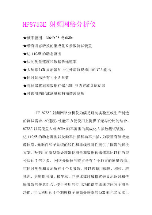
E8753E S8753D说明书(总11页)-CAL-FENGHAI.-(YICAI)-Company One1-CAL-本页仅作为文档封面,使用请直接删除HP8753E 射频网络分析仪★频率范围:30kHz~3或6GHz★带有固态转换的集成化S参数测试装置★达110dB的动态范围★快的测量速度和数据传递速率★大屏幕LCD显示器加上供外部监视器用的VGA输出★同时显示所有4个S参数★将仪器状态和数据存储/调用到内置软盘驱动器★可选用的时域测量和扫描谐波测量HP 8753E射频网络分析仪为满足研制实验室或生产制造的测试需求,在速度、性能和方便使用上提供了无与伦比的结合。
8753E以其覆盖3或6GHz频率范围的集成化S参数测试装置、达110dB的动态范围以及频率扫描和功率扫描,为表征有源或无源网络、元器件和子系统的线性和非线性特性提供了圆满的解决方案。
所使用的新型微处理器使测量和数据传递速率比以往的型号快达7倍之多。
网络分析仪的特点是有2个独立的测量通道,可同时测量和显示所有4个S参数。
可以选择用幅度、相位、群延迟、史密斯圆图、极坐标、驻波比或时域格式来显示反射和传输参数的任意组合。
便于使用的专用功能键能迅速访问各个测量功能。
可以利用达4个刻度格子在高分辩率的LCD彩色显示器上以重叠或分离屏面的形式来观察测量结果。
为了驱动更大的外部监视器,以便于观察,增加了与VGA兼容的输出。
较好的通用性和性能一个集成化的合成源提供了达10mW的输出功率(用选件011可达100mW),1Hz的频率分辩率和线性频率,对数频率,列表频率,CW和功率扫描功能。
三个调谐接收机可以在6GHz(带有选件006频率扩展)处105dB或3GHz(标准)110dB的宽动态范围内进行独立的功率测量或同时比值测量。
集成化的测试装置可以在不使用倍频器的情况下,测量达6GHz装置的传输和反射特性。
为了在非同轴系统中进行方便而精确的测量,特提供了TRL*/LRM*1校准。
8753D网络分析仪学习教材
网络分析仪操作规范
SH875D仪器的操作步聚:
1.开机前接好地线与稳压器。
2.打开电源开关(OPEN)
3.设置测试天线所需要的频率FORQ→设置开始频率(START)→设置终
止频率(STOP)
4.校准(CAL)→选择Carlibrate Menu→选择Reflection 1-Port
联接开路器按Open,取下开路键
联接短路器按Shopts,取下短路键
联接50Ω负载按Load→ Done,等仪器自动校准完毕。
5.取所须Marker(点)→看SMITH CHART ,正常的为50欧,不超过正负
0.1。
如果超过正负0.1,则仪器必须重新校准到准确为止,如一直校不
准,则按复位键(Preset)重新校正.
6.显示选择(DISPLAY)→记忆当前数据和记忆显示当前数据(DATA→
MEMORY)[第7个键] →显示记忆数据和当前数据(DATA and MEMORY)[第4个键]或只显示当前记忆(MEMORY)[第3个键],如不显示记忆图→按不显示图形(DISPLAY:DATA)[第2个键。
尤勇
2010年5月31。
agilent信号分析仪操作步骤.doc
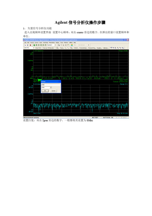
Agilent信号分析仪操作步骤1,矢量信号分析仪功能进入出现频率设置界面设置中心频率:双击center旁边的数字,在弹出的窗口设置频率和单位。
设置扫宽:双击Span旁边的数字,一般都将其设置为8Mhz设置range 单击range旁边的数字按向下键将波形图调至中心位置。
(-20dbm左右)选择菜单中的MeasSetup——Demodulator——Digital Demod。
进入数字信号分析功能。
选择图形个数查看星座图(双击左侧绿色方框,在弹出的对话框中选择constellation)查看I眼图(双击左侧绿色方框,在弹出的对话框中选择I-Eye)查看Q眼图(双击左侧绿色方框,在弹出的对话框中选择Q-Eye)进入扫频仪后界面如下设置起始频率,选择功能键Stop Freq设置终止频率,选择Center Freq设置中心频率。
按控制面板上的SPAN x Scale键出现如下界面,选择功能键Span设置扫宽按控制面板上的AMPTD y Scale键出现如下界面,选择功能键More 1of2选择Y Axis Unit 设置电平的单位。
按控制面板上的Trace Delecter键,选择功能键盘Trace Average后出现平滑的曲线。
按控制面板上的Input/Output键,选择功能键RF Input [AC,50欧],选择75欧。
按控制面板上的BW键,出现如下界面。
分别对RBW和VBW进行设置使曲线接近平滑,建议RBW设置为500-600khz左右,VBW设置为20khz左右,这样兼顾了曲线的平滑与扫频的速度。
按控制面板上的Maker 键后输入频率与单位,设置游标。
按控制面板上的Maker Function后可以选择有一定带宽范围的游标,出现如下界面。
选择功能键Band/Interval Density。
选择功能键Band Adjust调整宽度,如需关闭选择Maker Function Off。
安捷伦网络分析报告仪使用手册簿
标准文档网络分析仪使用手册目录ACTIVE CH/TRACE Block:Channel Prev:选择上一个通道 Channel Next:选择下一个通道Trace Prev:选择上一个轨迹 Trace Next:选择下一个轨迹RESPONSE Block:Channel Max: 通道最大化Trace Max: 轨迹最大化Meas: 设置S参数Format: 设置格式Scale: 设置比例尺Display: 设置显示参数Avg: 波形平整Cal: 校准STIMULUS Block:Start: 设置频段起始位置Stop: 设置频段截止位置Center: 设置频段中心位置Span: 设置频段范围Sweep Setup: 扫描设置Trigger: 触发NAVIGATION Block: Enter: 确定ENTRY Block:Entry off: 取消当前窗口Back space: 退格键Focus: 窗口切换键+/-: 正负切换键G/n, M/,k/m: 单位输入INSTR STATE Block:Macro Setup:Macro Run:Macro Break:Save/Recall: 程序载入载出键 System: 系统功能键Preset: 预设置键MKR/ANALYSIS Block:Marker: 标记键Marker Search: 标记设置键Marker Fctn: 标记功能Analysis: 分析部分按键详细功能:------------------------------------------------------------ System: (系统功能设定)Print: 将显示屏画面打印出来Abort printing: 终止打印Printer setup: 配置打印机Invert image: 颠倒图象颜色Dump screen image: 将显示屏画面保存到硬盘中E5091A setup: 略Misc setup: 混杂功能Beeper: 发声控制Beeper complete: 开/关提示音Test beeper complete: 测试开/关提示音Beep warning: 开/关警告音Test beep warning: 测试开/关警告音Return: 返回GPIB setup: 略Network setup: 略Clock setup: 时钟设定Set date and time: 设置日期和时间Show clock: 开/关时间显示Return: 返回Key lock: 锁定功能Front panel & keyboard lock: 锁定前端面板和键盘Touch screen & mouse lock: 锁定触摸屏和鼠标Return: 返回Color setup: 颜色设定Normal: 设置普通模式下的颜色设定Data trace1: 对数据轨迹1进行颜色设定Red: 调整数据轨迹1红色分量的大小Green: 调整数据轨迹1绿色分量的大小Blue: 调整数据轨迹1蓝色分量的大小Return: 返回Data trace2—Data trace 9: 数据轨迹2到数据轨迹9的颜色设定方法同数据轨迹1Mem trace1—Mem trace 9: 记忆轨迹1到记忆轨迹9的颜色设定方法同数据轨迹1Graticule main: 调整方格标签和外部筐架的颜色设定(设定方法同前)Graticule sub: 调整方格线的颜色设定(设定方法同前)Limit fail: 调整限制测试中失败标签的颜色设定(设定方法同前)Limit line: 调整限制线的颜色(设定方法同前)Background: 调整背景颜色(设定方法同前)Reset color: 使用默认颜色设置Return: 返回Invert: 设置颠倒颜色后的颜色设置Return: 返回Channel trace setup: 略Control panel: 略Return: 返回Backlight: 略Firmware revision: 略Service menu: 略Return: 返回-----------------------------------------------Trigger: (触发设定)Hold: 当前通道停止扫描Single: 进行一次扫描后停止Continuous: 连续扫描Hold all channels: 所有通道停止扫描Continuous disp channels: 对所有通道进行连续扫描Trigger source: 略Restart: 终止一次扫描Trigger: 略Return: 返回-----------------------------------------------Marker: (标记设定)Maker 1:激活标记1,并出现窗口设置其值Maker 2:激活标记2,并出现窗口设置其值Maker 3:激活标记3,并出现窗口设置其值Maker 4:激活标记4,并出现窗口设置其值More markers: 更多的标记Maker 5-9: 用法同前Return: 返回Ref marker: 激活参考标记,并出现窗口设置其激励值Clear marker menu: 清除标记菜单All off: 全部清除Maker 1: 清除标记1Maker 2-9: 同上Ref marker: 清除参考标记Return: 返回Maker → Ref marker: 将激活标记设置成参考标记Ref marker mode: 设置为参考标记模式Return: 返回----------------------------------------------- Marker Fctn: (标记功能设定)Marker → start: 设定标记的起始激励值Marker → stop: 设定标记的截止激励值Marker → center: 设定标记的中心激励值Marker → reference:略Marker → delay: 略Discrete: 略Couple: 略Marker table: 调出标记列表Statistics: 显示三项统计数据Return: 返回----------------------------------------------- Marker search: (标记搜索设定)Max: 将标记移到其轨迹上的最大点Min: 将标记移到其轨迹上的最小点Peak: 峰值功能Search peak: 寻找顶峰Search left: 在左侧寻找顶峰Search right: 在右侧寻找顶峰Peak excursion: 设置顶峰偏移Peak polarity: 极性设置Positive: 正极性Negative: 负极性Both: 双极性Cancel: 取消Return: 返回Target: 目标搜索功能Search target: 寻找目标Search left: 向左寻找目标Search right: 向右寻找目标Target value: 设定目标值Target transition: 根据变化趋势寻找目标Positive: 正向搜索Negative: 负项搜索Both: 双向搜索Cancel: 取消Return: 返回Tracking: 跟踪Search range: 搜索范围菜单Search range: 关闭或开启局部搜索功能Start: 设定搜索范围起始频率Stop: 设定搜索范围截至频率Couple: 略Return: 返回Bandwidth: 关闭或开启带宽搜索功能Bandwidth value: 设定带宽值Return: 返回-----------------------------------------------Meas: (s参数的设定)S11: 1端口发1端口收S12: 1端口发2端口收S21: 2端口发1端口收S22: 2端口发2端口收Return: 返回注:以上收发均针对网络测试仪而言,对被测产品来说刚好相反-----------------------------------------------Scale: ( 刻度标尺的设定)Auto scale: 自动调整刻度标尺Auto scale all: 对所有自动调整标尺Divisions: 设定格子的个数 (必须为偶数个)Scale/Div: 设定每格所代表的值Reference position: 确定参考线位置Reference value: 设定参考线值Marker reference: 将当前激活标记的响应值设为参考线Electrical delay: 对激活的轨迹设置一个延迟Phase offset: 测试相位时添加相位偏移Return: 返回-----------------------------------------------Save/Recall: (保存,装载设定)Save state: 存储当前状态State01—state08: 将当前状态存于状态01到状态08Autorec: 以Autorec为文件名将当前状态储存于硬盘中File dialog: 以任意文件名将当前状态保存于硬盘中Return: 返回Recall state: 装载已保存状态State01-state08: 装载状态01到状态08Autorec: 装载以文件名Autorec保存的状态File dialog: 装载以其它文件名保存的状态Return: 返回Save channel:State A – State D: 将当前所有通道设定保存到状态A到D中Clear states: 清除所有通道设定记录Ok: 确定Cancel: 取消Return: 返回Recall channel: 装载通道设定State A – State D: 将状态A到D中保存的通道设定装载出来Return: 返回Save type: 设定存储类型State only: 只保存设定数据State & Cal: 保存设定和校验数据State & Trace: 保存设定和轨迹数据All: 保存所有数据Cancel: 取消Channel/Trace: 略Save trace data: 保存轨迹数据Explore...: 略Cancel: 取消----------------------------------------------- Display:(显示设定)Allocate Channels: 设置屏幕显示通道方式Numbers of traces: 设置轨迹数目Allocate traces: 设置显示轨迹方式Display: 即时波形与记忆波形的显示设置Data: 只显示即时波形Mem: 只显示记忆波形Data&Mem: 同时显示两种波形Off: 两种波形都不显示Cancel: 取消Data Mem: 记忆波形Data Math: 选择数据处理的类型Off: 关闭数据处理功能Data/Mem: 即时波形除以记忆波形Data*Mem: 即时波形乘以记忆波形Data-Mem: 即时波形减去记忆波形Data+Mem: 即时波形加上记忆波形Cancel: 取消Edit Title Label: 编辑标题标签Title Label: 显示/不显示标题Graticule Label: 略Invert Color: 反转颜色,以白色为背景色Frequency: 显示/不显示频率Update: 略Return: 返回----------------------------------------------- Format: (格式设定)Log Mag: Y轴以对数形式显示振幅,X轴显示频率Phase: Y轴以对数形式显示相位,X轴显示频率Group Delay: Y轴以对数形式显示群时延,X轴显示频率Smith: 史密斯圆图的格式设置Polar: 极性图的格式设置Lin Mag: Y轴以线性形式显示振幅,X轴显示频率SWR: Y轴显示驻波比,X轴显示频率Real: : Y轴显示实部,X轴显示频率Imaginary: : Y轴显示虚部,X轴显示频率Expand Phase: Y轴显示扩展相位,X轴显示频率Positive Phase: Y轴显示正相位,X轴显示频率Return: 返回----------------------------------------------- Sweep Setup: (扫描设定)Power: 打开激励信号输出设置菜单Power: 设置网络分析仪内部信号源的输出电平Power Ranges: 选择电平范围Port Couple: 在现有电平上打开/关闭端口耦合Port Power: 当端口耦合关闭时设置端口功率Slope [xx dB/Hz]: 略Slope [ON/OFF]: 略CW Freq: 设置功率扫描的固定频率RF Out: 开/关激励源的输出Return: 返回Sweep Time: 设置端口扫描时间Sweep Delay: 设置扫描延时Sweep Mode: 选择扫描模式Points: 设置每次扫描的扫描点数Sweep Type: 选择扫描类型Edit Segment Table: 编辑段扫描设置表Freq Mode: 切换频率设置模式List IFBW: 在分段表中显示/不显示中频带宽List Power: 在分段表中显示/不显示功率List Delay: 在分段表中显示/不显示延时List Sweep Mode: 在分段表中显示/不显示扫描模式List Time: 在分段表中显示/不显示扫描时间Delete: 删除表项Add: 增加表项Clear Segment Table: 清除分段表Export to CSV File: 将限制表格输出以CSV文件格式保存Import from CSV File: 从CSV格式文件中输入限制表格Return: 返回Segment Display: 略Return: 返回-----------------------------------------------Avg:(平滑设定)Averaging Restart: 复位计数器从1开始Avg Factor: 设置均衡因子Averaging: 开启/关闭平滑功能Smo Aperture: 略Smoothing: 开启/关闭平整功能IF Bandwidth: 设置中频带宽Return: 返回-----------------------------------------------Cal: (校验设定)Correction: 开启/关闭错误修正Calibrate: 校验菜单Response (Open): 开路响应校验选择菜单Select Port: 选择端口Open: 对选定端口进行开路条件下的响应校验(用于消除响应跟踪误差)Load (Optional): 对选定端口进行负载条件下的隔离度校验(用于消除方向性误差)Done: 终止校验进程并计算校验系数Cancel: 取消Return: 返回Response (Short): 短路响应校验选择菜单Select Port: 选择端口Short: 对选定端口进行短路校验(用于消除反射跟踪误差)Load (Optional): 对选定端口进行负载条件下的隔离度校验(用于消除方向性误差)Done: 终止校验进程并计算校验系数Cancel: 取消Return: 返回Response (Thru): 传输响应校验选择菜单Select Port: 选择端口Thru: 对选定端口进行传输响应校验(用于消除传输跟踪误差)Isolation (Optional): 对选定端口进行隔离度校验(用于消除隔离度误差)Done: 终止校验进程并计算校验系数Cancel: 取消Return: 返回1-Port Cal: 单个端口校验菜单Select Port: 选择端口Open: 对选定端口进行开路校验Short: 对选定端口进行短路校验Load: 对选定端口进行负载校验Done: 终止校验进程并计算校验系数Cancel: 取消Return: 返回2-Port Cal: 双端口校验菜单Select Ports: 选择端口Reflection: 反射校验菜单Transmission: 传输校验菜单Isolation (Optional): 隔离度校验菜单Done: 终止校验进程并计算校验系数Cancel: 取消Return: 返回ECal: 电子校验菜单1—Port ECal: 单端口电子校验2—Port ECal: 双端口电子校验Thru ECal: 传输电子校验Isolation: 开启/关闭隔离度校验功能Characterization: 电子校验特性选择菜单Characterization Info: 相应电子校验特性信息Confidence Check: 略Return: 返回Property: 显示/不显示校验属性Cal Kit: 选择校验组件Modify Cal Kit: 改变校验组件定义菜单Defines STDs: 定义校验组件的标准Specify CLSs: 指定标准种类Label Kit: 用户自定义组件Restore Cal Kit: 保存校验组件定义Return: 返回Port Extensions: 扩展端口菜单Velocity Factor: 设定速率因子Power Calibration: 功率校验菜单Select Port: 选择端口Correction: 开/关电平误差修正Take Cal Sweep: 进行功率校验数据的测量Abort: 终止功率校验数据的测量Use Sensor: 选择功率校验数据测量的功率传感器通道Num of Readings: 设定每个测量点的电平数目(平滑因子)Loss Compen: 损耗修正设定菜单Sensor A Settings: 设定通道A的功率传感器校验系数Sensor B Settings: 设定通道B的功率传感器校验系数Return: 返回Return: 返回-----------------------------------------------Analysis:Fixture Simulator: 略Gating: 略Transform: 略Conversion: 略Limit test: 测试限制菜单Limit test: 开启/关闭测试限制功能Limit line: 开启/关闭限制线功能Edit limit line: 编辑限制线Delete: 删除限制线Add: 添加限制线Clear Limit Table: 清除限制表格Export to CSV File: 将限制表格输出以CSV文件格式保存Import from CSV File: 从CSV格式文件中输入限制表格Return: 返回Fail Sign: 显示/不显示测试失败标记Return: 返回Return: 返回。
8753E 8753ES 8753D说明书
HP8753E 射频网络分析仪★频率范围:30kHz~3或6GHz★带有固态转换的集成化S参数测试装置★达110dB的动态范围★快的测量速度和数据传递速率★大屏幕LCD显示器加上供外部监视器用的VGA输出★同时显示所有4个S参数★将仪器状态和数据存储/调用到内置软盘驱动器★可选用的时域测量和扫描谐波测量HP 8753E射频网络分析仪为满足研制实验室或生产制造的测试需求,在速度、性能和方便使用上提供了无与伦比的结合。
8753E以其覆盖3或6GHz频率范围的集成化S参数测试装置、达110dB的动态范围以及频率扫描和功率扫描,为表征有源或无源网络、元器件和子系统的线性和非线性特性提供了圆满的解决方案。
所使用的新型微处理器使测量和数据传递速率比以往的型号快达7倍之多。
网络分析仪的特点是有2个独立的测量通道,可同时测量和显示所有4个S参数。
可以选择用幅度、相位、群延迟、史密斯圆图、极坐标、驻波比或时域格式来显示反射和传输参数的任意组合。
便于使用的专用功能键能迅速访问各个测量功能。
可以利用达4个刻度格子在高分辩率的LCD彩色显示器上以重叠或分离屏面的形式来观察测量结果。
为了驱动更大的外部监视器,以便于观察,增加了与VGA兼容的输出。
较好的通用性和性能一个集成化的合成源提供了达10mW的输出功率(用选件011可达100mW),1Hz的频率分辩率和线性频率,对数频率,列表频率,CW和功率扫描功能。
三个调谐接收机可以在6GHz(带有选件006频率扩展)处105dB或3GHz(标准)110dB的宽动态范围内进行独立的功率测量或同时比值测量。
集成化的测试装置可以在不使用倍频器的情况下,测量达6GHz装置的传输和反射特性。
为了在非同轴系统中进行方便而精确的测量,特提供了TRL*/LRM*1校准。
利用内置适配器移去校准技术,还能实现对非插入式器件的高精度测量。
高稳定度的频率基准(选件1D5)提高了对高Q器件,如表面声波(SAW)器件、晶体谐振器或介质谐振滤波器的频率测量精度。
8753ES网络分析仪使用手册--final

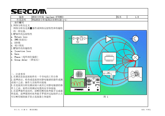
8753ES⽹络分析仪使⽤⼿册--final儀器網絡分析儀(Agilent 8753ES)版本 1.0作業說明VNA網絡分析儀測試基礎知識<1-1>⼀.操作說明1.⽹络分析仪定义⽹络分析仪是测量器件或⽹络反射特性和传输特的⼀种仪器。
2.RF器件的反射特性a. Return lossb. SWR(驻波⽐)c. S参数d. 端⼝阻抗2.RF器件的传输特性a. Issertion lossb. Gainc. Phase(线性相位偏移)d. Group delay (群延迟)⼆.注意事项1.在测试设备前⾯始终有⼀个导电的⼯作台垫2.进⾏清洁、检查或连接到对静电敏感的器件或测试端⼝之前,操作⼈员始终应接地3.在连接到分析仪测试端⼝或其它对静电敏感的器件上之前,始终应将测试电缆的内导体接地4.在进⾏器件连结时,请利⽤利⽤扭⼒扳⼿完成最终连接,进⾏紧固时扭⼒扳⼿不要冲过起始停⽌点可以利⽤辅助扳⼿防⽌连接器主体旋转图 1儀器網絡分析儀(Agilent 8753ES)儀器網絡分析儀(Agilent 8753ES)儀器網絡分析儀(Agilent 8753ES)⼆.注意事项儀器網絡分析儀(Agilent 8753ES)儀器網絡分析儀(Agilent 8753ES)4132儀器網絡分析儀(Agilent 8753ES)2134儀器網絡分析儀(Agilent 8753ES)点击右⾯板图 9儀器版本網絡分析儀(Agilent 8753ES) 1.0作業說明VNA網絡分析儀操作步骤<3-2>⼀.操作說明2.校准a.⽬的:消除仪器及连接电缆等带来的系统误差b.校准器件:如图9c.校准类型:1-port校准:测量反射特性时必须校准2-port校准:消除全部误差,是最完整,最精确的校准。
测量反射特性和传输特性时必须校准d.校准项⽬:开路校准,短路校准:只适于反射特性直通校准:只适于传输特性⼆.注意事项1.在测试设备前⾯始终有⼀个导电的⼯作台垫2.进⾏清洁、检查或连接到对静电敏感的器件或测试端⼝之前,操作⼈员始终应接地3.在连接到分析仪测试端⼝或其它对静电敏感的器件上之前,始终应将测试电缆的内导体接地4.在进⾏器件连结时,请利⽤利⽤扭⼒扳⼿完成最终连接,进⾏紧固时扭⼒扳⼿不要冲过起始停⽌点可以利⽤辅助扳⼿防⽌连接器主体旋转图 10儀器版本網絡分析儀(Agilent 8753ES) 1.0作業說明VNA網絡分析儀操作步骤<3-3>⼀.操作說明e.校准步骤:1.打开Measurement Correction菜单按下2.选择校准组件类型 SELECT CAL KITCAL KIT 3.5mmD3.选择校准类型 CALIBRATE MENU FULL 2-PORT(全⼆端⼝误差修正)4.选择修正类型,按下 REFLECTION 把开路器连接到端⼝1上,待显⽰出来的记录线稳定后按下FORWARD:OPEN5.把短路器连接到端⼝1上,待显⽰出来的记录线稳定后按下FORWARD:SHORT6.把阻抗匹配负载连接到端⼝1上,待显⽰出来的记录线稳定后按下FORWARD:LOAD7.重复item4~6,但把校准组件连接到端⼝2上并按对应软键。
AgilentD网络分析仪操作指导书

2.按BEGIN键,屏幕出现子菜单,选择要测量的器件类型(放大器、滤波器、宽带无源器件、混频器或电缆—只适于选件100)。
3.将被测器件接至网络分析仪。
如果使用非默认标准(N型阴性)的校准标准,则必须选择连接器的类型,为此,按CAL,再按Cal Kit,然后选择适当的类型。
按PRESET键。当分析仪用PRESET键预置时,它将返回到一已知的工作状态。
1.按FREQ键,显示屏出现频率菜单。
2.设置频率低端,按Start,再按数字键和单位键,键入设定值。
3.设置频率高端,按Stop,再按数字键和单位键,键入设定值。
还可用Center和Span软键来设置频率范围。
1.按面板上的MENU键平菜单。
备注事项
10.使用放大的情况
11.改变系统阻抗
12.用BEGIN键配置测量
为了精确测量,在分析仪的RF OUT端口可能需要放大。当被测器件要求的输入功率超过了分析仪规定的最大输出功率时,应使用放大。
分析仪具有50Ω或75Ω的特性阻抗,也可以改变为其它阻抗。为改变系统的阻抗,按CAL,More Cal,System Z0,50Ω或75Ω或其它。
2.按Level,再按数字键和单位键,键入功率电平设定值。
当电源关断时,输入的测量参数将保存在分析仪的存储器中,当电源重新接通时,这些参数将被恢复。
项目
操作步骤
操作方法
操作要求
备注事项
7.定度测量示迹
8.输入有效测量通道和测量类型
9.显示设定:
10.频率标记
11.参考方式
9.使用衰减的情况
SCALE键
利用数字键可为某一选定的参数输入特定的数值。用ENTER键或软件以适当的单位来终止数值输入。还可用面板旋钮实现对参数值的连续调节,还可用步进键改变数值。
Agilent软件操作说明书1.1
Agilent软件操作说明书Agilent软件操作说明书 (1)1 概述 (2)更新时间 (2)版本 (2)更新内容 (2)2008.9.15 (2)V1.1 (2)1.添加License申请 (2)2.添加软件存在问题总结 (2)3.添加前台reporter应用功能 (2)2 功能介绍 (2)2.1 License的安装 (2)2.2 运行软件 (5)2.3 创建工程 (6)2.4 设备添加..................................................................................... 错误!未定义书签。
2.5 导入基站数据 (16)2.6 测试过程中的界面试图 (22)2.7 测试脚本的配置 (28)2.7.1 Call_Control (29)2.7.2 FTP下载 (30)2.8 Report的分析 (35)2.9 数据卡的使用 (40)3 附件 (44)1概述通过Agilent软件能够对该地区的3G网络的进行测试,包括语音电话,视屏电话,FTP下载等,结合测试结果发现3G网络中存在的问题,为3G的网络优化提供必要的依据。
2功能介绍2.1 License的安装在运行软件之前需要安装license得到软件的使用权。
如何获取Agilent E6474 License1.若无License,则MapX不能正确显示2.选择Programe File/Agilent Wireless Solution/E6474-X/Utilities/License Manager3.选择Commuter License中的Remote Commuter License,得到Current Computer 的MachineCode,发送给相关人员获取License.中Load并安装,即OK2.2 运行软件如上图所示,打开软件后出现上图所示的界面,点击红色区域中的Collect data now按钮进入软件。
8753网络分析仪使用讲解书 繁体版
8753網絡分析儀使用講解一、儀器簡介8753為美國安捷掄科技公司生產用於高頻測試的射頻網絡分析儀,最低分辨頻率可達到1Hz,最大測試頻率達6G,掃描時間不超過40ms,最大輸出功率達13dB.它有8753ES和8753ET兩種型號,常用來測試的參數有插入損耗(Insertion Loss),回波損耗(Return Loss),駐波比(VSWR),目前在NBC的天線測試中主要測試駐波比(VSWR).二、高頻理論簡介目前主要測試的為插入損耗和回波損耗插入損耗公式如下圖回波損耗隻要由反射系數決定,公式如下三、儀器面板上常用控制鍵說明1 preset 使儀器處在預設狀態2 meas 設置傳輸方式3 start 設置儀器的起點頻率4format 設置儀器的反射參數,如回損,駐波比等5save/ recall 存儲和調用測試程序6display 屏幕的參數設置7scale 設置刻度8marker 顯示相應頻率的測試值9 cal 校正四、測試程序的調用和校正調用操作步驟如下(preset)----------(save recall) ----------選擇相應的程序----------recall state調用完後需進行校正,校正操作步驟如下(cal ) ----------calibrate menu-----------s11 1-port---------接入open 校正器後按open---------接入short校正器後按short-------------接入load校正器後按load----------done 1-port cal五、測試程序的新增若儀器無所需要的測試程序,則必須按以下操作步驟新增程序(以測試條件2.4G到2.5G, VSWR<2為例)打上括號的表示為儀器面板上的硬鍵,否則為儀器屏幕旁的8個軟鍵中的其中一個1 進入儀器預設狀態( preset)----------2 設定起點頻率(start)----------2.4----------GHz3 設定終點頻率----------(stop)----------2.5----------GHz4選擇1通道測試5----------(chan1)-6 設定測量參數為駐波比---------(meas)----------ref1:fwd s11(A/R)------(format)----------swr 7 設置駐波比刻度----------(scale)----------0.4----------enter8 進入判定線編輯菜單(system)----------limit menu------limit line--------limit line _On off---------limit test _On off---------beep fail _On off---------edit limit line刪除原有的判定線(若原來無判定線可省略此步驟)----------delete ---------delete9 增加新的判定線----------add11 設置判定線的起點頻率--------stimulus value--------2.4G--------12 設置判定線的起始駐波比值upper limit ----------2----------*1----------13設置起點的類型(return) --------limit type------flat line------ (return)-------14 設置判定線的終點頻率add---------- stimulus value---------2.5------GHz----------15 設置判定線的終止駐波比值upper limit ----------2 ----------*1----------16 設置線的終點(return)------limit type-------single point------17 儲存成相應的料號文件(marker)---------- (save recall)----------save state ---------file utilities---------------rename file-------輸入相應的料號名----------done備注:1:此為8753ES 普通測試程序的編輯,,若為雙頻天線則需在16步後重復9到16的步驟2:2,3步驟中的頻率可隨意設置,如可設置start 2G,Hz,stop 3G,但此范圍一定要把判定線的頻率范圍.包括在內.3對於需測試用兩種規格的天線,還需要在第12步後按如下操作(display) ----------dual chan seup----------dual chan Onoff---------chan2---------ref1:fwd s11(A/R)----------format----------swr後重復6到16的步驟即可.六、常用注意事項1儀器電源需使用有接地保護的電源.2使用校正器使請注意動作要輕,請勿擰校正器後端.3測試時請注意要將轉接頭擰到位,轉接線固定好,校正完後請先用防呆用品進行防呆測試.,。
网络分析仪操作指导课件演示文稿【共24张PPT】

2024/3/26
b 2 = S 21 a 1 + S 22 a 2
4
➢ S11 = forward reflection coefficient (input match)
➢ S22 = reverse reflection coefficient (output match)
➢ S21 = forward transmission coefficient (gain or loss)
12
传输系数
传输电压与入射电平之比
2024/3/26
13
插入损耗与增益
➢ 增益:传输电压的绝对值大于入射电压的绝对值 ➢ 插入损耗:传输电压的绝对值小于入射电压的绝对值
➢ 传输系数的相位部分称为插入相位
2024/3/26
14
群延时
➢ 是相位失真的一个有用的度量。是信号通过被测器件的传 输时间随频率变化的量度。群时延可以由对被测器件的相 位响应随时间的变化取微分进行计算
2024/3/26
11
2.纯驻波状态
➢ 短路:负载阻抗ZL=0时,Γ=-1, RL=0,SWR →∞ 。 开路:负载阻抗ZL=∞, Γ=1, RL=0 ,SWR →∞
➢3.行驻波状态
当ZL≠Z0时,Γ<1,传输线上为“部分 行波”状态,“部分
反射”状态,此时负 载失配,导致传输线上出现部分驻波
2024/3/26
Incident
S 21
Transmitted
下面这a 1个图很直观的描述了S-parameter之间的关系,以及传输的形式。
S 11
b
2
Reflected
DUT
S 22
b1
Port 1
Agilent_8753D网络分析仪操作指导书
当电源关断时,输入的测量参数将保存在分析仪的存储器中,当电源重新接通时,这些参数将被恢复。
项目
操作步骤
操作方法
操作要求
备注事项
7.定度测量示迹
8.输入有效测量通道和测量类型
9.显示设定:
10.频率标记
11.参考方式
9.使用衰减的情况
SCALE键
1.选中刚才建立的目录名“×××”;
2. 依次按下屏幕上的软按键Save State(根据文件数目的需要,可以建立多个,但最多可建7个,如按一下为创建一个文件),File Utilities,Rename File,将刚才创建的文件取文件名为“★★★”(可以自己取名,比如LPA0800-035)。
3.按下Enter,文件即可建立完成。
最大输入电平:+10dBm
损坏电平:±26dBm或35Vdc
阻抗:50Ω(用选件075时为75Ω)
在PORT2联接50DB高功率衰减器的情况下
针对目前的线性功放
备注事项
10.使用放大的情况
11.改变系统阻抗
12.用BEGIN键配置测量
为了精确测量,在分析仪的RF OUT端口可能需要放大。当被测器件要求的输入功率超过了分析仪规定的最大输出功率时,应使用放大。
分析仪具有50Ω或75Ω的特性阻抗,也可以改变为其它阻抗。为改变系统的阻抗,按CAL,More Cal,System Z0,50Ω或75Ω或其它。
这组信号源键可选择所希望送到被测件上的源输出信号。这组信号源键还控制扫描时间、点数及扫描触发。
这组配置键控制接收机和显示器的参数,包括接收机带宽和平均,显示刻度和格式、标记功能以及仪器校准等。
安捷伦8753网络分析仪操作指导
8753网络分析仪表培训资料
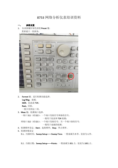
一、参数设置
1、仪表按键区绿色按钮Preset键,
重新建立一张新表;
2、Format键,进行检测功能选择。
Log Mag:衰减;
SWR:驻波或TDR;
Real:回损。
一般只用到这三项。
3、Meas键:检测端口选择。
一端口S11(或S22):一个端口发射信号和接收信号,
一般用于驻波和TDR检测;
两端口S12(或S21):一个端口发射信号,另一个端口接收信号,
一般用于衰减的检测。
4、检测频率设定:Start:起始频率;Stop:终止频率。
5、检测参数设定
5.1、扫描时间:Sweep Setup——Sweep Time:一般衰减为5秒,驻波为1秒。
5.2、扫描点数:Sweep Setup——Points:一般衰减为801点,驻波为1601点。
扫描时间,修改为1s
扫描点数,修改为1601
5.3、带宽:Avg——IF Bandwidth:一般为3KHz。
带宽,修改为3000Hz
5.4显示比例:Scale——Scale/Div,一般驻波最高为1.5时设置为50m/div;衰减可根据实际
情况进行调整。
修改为50m/div
二、校表Cal键
1、Cal Kit:校准组件选择。
N型校准件一般选85032F或85032B/E。
2、Calibrate:1-Port Cal:单端口校准;2-Port Ca l:双端口校准,Respinse(Thru):衰减校准。
安捷伦网络分析仪使用教程

Q
AM (dB)
Mag(AM out)
AM - PM Conversion =
Mag(PMout) Mag(AMin)
(deg/dB)
PM (deg)
Mag(PM out)
I
Output Response
Time
AM to PM conversion can cause bit errors
page 20
page 17
器件的功率动态范围:
输入1dB 输入1dB压缩点 1dB压缩点
CH1 S21 C2 1og MAG 1 dB/ REF 32 dB 30.991 dB 12.3 dBm
0 1dB
point: 1 dB compression point 输入功率增加导致器件增益下降1dB 输入功率增加导致器件增益下降1dB 相对测试 输出1dB压缩点(绝对测试) 1dB压缩点 输出1dB压缩点(绝对测试)
Load Power (normalized)
1 0.8 0.6 0.4 0.2 0 0 1 2 3 4 5 6 7 8 9 10
Zs = R + jX
RL / RS
ZL = Zs* = R - jX
RL = RS: 负载上最大功率传输
page 8
传输特性
V
输入
V
DUT
传输
传输系数 =
Τ
=
VTransmitted VIncident V V
Agilent 系列 网络分析仪
page 1
网络分析仪
网络分析仪测试基本概念 网络分析仪 工作原理 误差和校准 ENA PNA
page 2
系统组成及器件功能
LNA SAW 滤波器 平衡/非平衡转换 天线 双功器 功分器 射频前端模块 混频器 LO LC 滤波器
8753E8753ES8753D说明书
HP8753E 射频网络分析仪★频率范围:30kHz~3或6GHz★带有固态转换的集成化S参数测试装置★达110dB的动态范围★快的测量速度和数据传递速率★大屏幕LCD显示器加上供外部监视器用的VGA输出★同时显示所有4个S参数★将仪器状态和数据存储/调用到内置软盘驱动器★可选用的时域测量和扫描谐波测量HP 8753E射频网络分析仪为满足研制实验室或生产制造的测试需求,在速度、性能和方便使用上提供了无与伦比的结合。
8753E以其覆盖3或6GHz频率范围的集成化S参数测试装置、达110dB的动态范围以及频率扫描和功率扫描,为表征有源或无源网络、元器件和子系统的线性和非线性特性提供了圆满的解决方案。
所使用的新型微处理器使测量和数据传递速率比以往的型号快达7倍之多。
网络分析仪的特点是有2个独立的测量通道,可同时测量和显示所有4个S参数。
可以选择用幅度、相位、群延迟、史密斯圆图、极坐标、驻波比或时域格式来显示反射和传输参数的任意组合。
便于使用的专用功能键能迅速访问各个测量功能。
可以利用达4个刻度格子在高分辩率的LCD彩色显示器上以重叠或分离屏面的形式来观察测量结果。
为了驱动更大的外部监视器,以便于观察,增加了与VGA兼容的输出。
较好的通用性和性能一个集成化的合成源提供了达10mW的输出功率(用选件011可达100mW),1Hz的频率分辩率和线性频率,对数频率,列表频率,CW和功率扫描功能。
三个调谐接收机可以在6GHz(带有选件006频率扩展)处105dB或3GHz(标准)110dB的宽动态范围内进行独立的功率测量或同时比值测量。
集成化的测试装置可以在不使用倍频器的情况下,测量达6GHz装置的传输和反射特性。
为了在非同轴系统中进行方便而精确的测量,特提供了TRL*/LRM*1校准。
利用内置适配器移去校准技术,还能实现对非插入式器件的高精度测量。
高稳定度的频率基准(选件1D5)提高了对高Q器件,如表面声波(SAW)器件、晶体谐振器或介质谐振滤波器的频率测量精度。
8753ES网络分析仪使用手册--final
儀器網絡分析儀(Agilent 8753ES)版本 1.0作業說明VNA網絡分析儀測試基礎知識<1-1>一.操作說明1.网络分析仪定义网络分析仪是测量器件或网络反射特性和传输特的一种仪器。
2.RF器件的反射特性a. Return lossb. SWR(驻波比)c. S参数d. 端口阻抗2.RF器件的传输特性a. Issertion lossb. Gainc. Phase(线性相位偏移)d. Group delay (群延迟)二.注意事项1.在测试设备前面始终有一个导电的工作台垫2.进行清洁、检查或连接到对静电敏感的器件或测试端口之前,操作人员始终应接地3.在连接到分析仪测试端口或其它对静电敏感的器件上之前,始终应将测试电缆的内导体接地4.在进行器件连结时,请利用利用扭力扳手完成最终连接,进行紧固时扭力扳手不要冲过起始停止点可以利用辅助扳手防止连接器主体旋转图 1儀器網絡分析儀(Agilent 8753ES)儀器網絡分析儀(Agilent 8753ES)儀器網絡分析儀(Agilent 8753ES)二.注意事项儀器網絡分析儀(Agilent 8753ES)儀器網絡分析儀(Agilent 8753ES)4132儀器網絡分析儀(Agilent 8753ES)2134儀器網絡分析儀(Agilent 8753ES)点击右面板图 9儀器版本網絡分析儀(Agilent 8753ES) 1.0作業說明VNA網絡分析儀操作步骤<3-2>一.操作說明2.校准a.目的:消除仪器及连接电缆等带来的系统误差b.校准器件:如图9c.校准类型:1-port校准:测量反射特性时必须校准2-port校准:消除全部误差,是最完整,最精确的校准。
测量反射特性和传输特性时必须校准d.校准项目:开路校准,短路校准:只适于反射特性直通校准:只适于传输特性二.注意事项1.在测试设备前面始终有一个导电的工作台垫2.进行清洁、检查或连接到对静电敏感的器件或测试端口之前,操作人员始终应接地3.在连接到分析仪测试端口或其它对静电敏感的器件上之前,始终应将测试电缆的内导体接地4.在进行器件连结时,请利用利用扭力扳手完成最终连接,进行紧固时扭力扳手不要冲过起始停止点可以利用辅助扳手防止连接器主体旋转图 10儀器版本網絡分析儀(Agilent 8753ES) 1.0作業說明VNA網絡分析儀操作步骤<3-3>一.操作說明e.校准步骤:1.打开Measurement Correction菜单按下2.选择校准组件类型 SELECT CAL KITCAL KIT 3.5mmD3.选择校准类型 CALIBRATE MENU FULL 2-PORT(全二端口误差修正)4.选择修正类型,按下 REFLECTION 把开路器连接到端口1上,待显示出来的记录线稳定后按下FORWARD:OPEN5.把短路器连接到端口1上,待显示出来的记录线稳定后按下FORWARD:SHORT6.把阻抗匹配负载连接到端口1上,待显示出来的记录线稳定后按下FORWARD:LOAD7.重复item4~6,但把校准组件连接到端口2上并按对应软键。
双工器的网络分析仪测试指导

Product Note8753ES Vector Network Analyzer AgilentTesting Duplexers Using an Agilent 8753ESOption H39 Three-port Network AnalyzerTable of ContentsIntroduction . . . . . . . . . . . . . . . . . . . . . . . . . . . . . . . . . . . . . . . . . . . . .3Equipment required . . . . . . . . . . . . . . . . . . . . . . . . . . . . . . . . . . . . . . . .4Duplexer connection diagram . . . . . . . . . . . . . . . . . . . . . . . . . . . . . . .5Section A.Measure antenna-to-receiver and transmitter-to-antennainsertion loss . . . . . . . . . . . . . . . . . . . . . . . . . . . . . . . . . . . . . . . . . . .6Section B.Measure antenna match . . . . . . . . . . . . . . . . . . . . . . . . . . . . . . . . .11Section C.Measure receiver-to-transmitter isolation and receiverand transmitter match . . . . . . . . . . . . . . . . . . . . . . . . . . . . . . . . . . .16Accuracy considerations of a three-port measurement . . . . . . .18Example: Receiver-to-transmitter isolation . . . . . . . . . . . . . . . .19Example: Coupler isolation . . . . . . . . . . . . . . . . . . . . . . . . . . . . .218753ES Option H39 specifications . . . . . . . . . . . . . . . . . . . . . . . . . . . .22Questions and answers . . . . . . . . . . . . . . . . . . . . . . . . . . . . . . . . . . . .23Duplexers are three-port filters that are used in many communication sys-Introductiontems. They allow a single antenna to be shared between separate transmitand receive signal paths. Since duplexers are three-port devices, theyprovide measurement challenges to traditional network analyzers with onlytwo ports. During alignment, it is essential to see both the transmitter-to-antenna (Tx–Ant) and antenna-to-receiver (Ant–Rx) paths, since tuningthe response of one path can affect the response of the other path.Option H39 adds a third test port to a standard 8753ES network analyzerto allow for single-connection measurements of duplexers. With OptionH39, you can simultaneously measure the insertion loss from Tx–Ant andfrom Ant–Rx. Simultaneous measurement of the insertion loss allowsobservation of path interactions. This eliminates retest and rework thatoccurs when only measuring one path at a time. In addition, isolationbetween the transmitter port and receiver port (Tx–Rx) and match of allthree ports can be measured.This product note describes the measurement process and accuracy con-siderations of testing a duplexer with high dynamic range using an 8753ESwith Option H39. The product note examines Ant–Rx, Tx–Ant and Tx–Rxinsertion loss and Ant, Rx, and Tx match measurements. Since the duplex-er has high dynamic range, swept-list frequency mode is used to optimizemeasurement speed. In addition, the challenges of testing three-portdevices such as couplers are discussed.The information in this product note is tailored to an 8753ES networkanalyzer with Option H39. However, most of the information is applicableto 8753ES with Z5621A H39 external three-port test set. To a lesserextent, the information is applicable to 8753ES with Z5621A H36 externalduplexer test set. For further differentiation of these options, refer to thequestions and answers section of this document.Figure 1. 8753ES Option H39 block diagram.Measurement paths Port 1 to port 2S 11, S 21, S 12, S 22Port 1 to port 3S 11, S 31, S 13, S 33Port 2 to port 3S 22, S 32, S 23, S 33The following equipment is required for the measurements described inthis note.•8753ES Option H39 (or 8753ES with Z5621A H39)•85033D calibration kit or appropriate calibration kit•Cables•Duplexer or three-port device under testAll measurements described in this note use the 8753ES Option H39 net-work analyzer. The reader should be familiar with general network analyzer operation. Refer to the 8753ES User’s Guide (part number 08753-90007)for a complete description of instrument operation.In the following measurement procedures, the 8753 front panel hard keys appear in brackets with bold type (for example [Display]). The “softkeys,”displayed on the screen, appear in italic type (for example, LOG MAG ).Block DiagramEquipment requiredConnect the network analyzer’s port 1 to the duplexer receiver port (Rx),the analyzer’s port 2 to the antenna port (Ant), and the analyzer’s port 3 to the transmitter port (Tx).Figure 2. Duplexer connection diagram.During the following sections, this product note provides detailed instruc-tions for testing an 800 MHz duplexer. Section A covers antenna-to-receiv-er and transmitter-to-antenna insertion loss measurements. Section B describes antenna match measurement. Section C covers receiver-to-transmitter isolation, and receiver and transmitter match measurements. In each section, the network analyzer stimulus is initially setup and then a calibration is performed. The product note provides the step-by-step list of keystrokes required for configuring the stimulus.Duplexer connection diagramConfigure the network analyzer to measure S 12and S 23on channels 1 and 2 respectively, as shown in Table 2. Channels 1 and 2 must be uncoupled,because each path requires a different calibration. In dual- or quad-channel mode, uncoupling the channels uncouples channels 1 and 3 from channels2 and 4.Table 2. Duplexer configuration for insertion loss measurement.Channel 1Channel 2S 12S 23Path 1–2 (Ant–Rx)Path 2–3 (Tx–Ant)Two-port calibration Two-port calibrationThe following keystrokes provide instructions for setting up themeasurements shown in Table 2. for a duplexer in the frequency range of 700–1000 MHz.[Preset]If you are using the Z5621A H39external test set, configure the net-work analyzer initially using [System], CONFIGURE MENU, USER SETTINGS, K39 MODE ON off . With an Option H39, the analyzer is auto-matically configured as a three-port test set.[Start][700 M/µ][Stop][1000 M/µ][Sweep Setup]COUPLED CH on OFF[Display]DUAL|QUAD SETUPDUAL CHAN ON offSPLIT DISPLAY 1X[Meas][Chan 1]SELECT PORTS [1-2]Trans: REV S 12(A/R) {Ant–Rx insertion loss}[Chan 2]SELECT PORTS [2-3]Trans: REV S 23(A/R) {Tx–Ant insertion loss}Title the channels. [Chan 1][Display]MORETITLEERASE TITLE“Ant –Rx insertion loss”[Chan 2]TITLEERASE TITLE“Tx –Ant insertion loss”Section A.Measure antenna-to-receiver and transmitter-to-antenna insertion lossAuto scale all channels. At this point, you should see the common duplexer response shown in Figure 3.Figure 3. Measurement of Ant–Rx and Tx–Ant insertion loss.Next set up the power level and IF bandwidth and number of points.The default power level, IF bandwidth, and number of points are 0 dBm, 3700 Hz, and 201 points.In this example, the duplexer has over 100 dB of dynamic range, so you need to use a narrow IF bandwidth in the stopband for accurate transmis-sion measurements. If you use a narrow IF bandwidth (for example 30 Hz) during the entire frequency sweep, the measurement time will be very long. Instead, use swept-list frequency mode to optimize speed and accura-cy. With swept-list mode, you divide the frequency span into multiple seg-ments. You can independently set the IF bandwidth in each segment. So in the stopband, use narrow bandwidths (slow sweep), and in the passband, use wide bandwidths (fast sweep). The swept-list mode setup for this measurement is shown in Table 3.If you are testing a combination of an amplifier and filter, you can also set the power level in each frequency segment independently to maximize dynamic range. For example, in the passband you can set the power level low (for example –30 dBm), and in the stopband, use maximum power (for example +10 dBm).[Chan 1][Sweep Setup]SWEEP TYPE MENUEDIT LISTADDSEGMENT: START[700 M/µ]SEGMENT: STOP[850 M/µ]STEP SIZE[2 M/µ] #You can either configurethe step size or thenumber of points. MORELIST IF BW ON offSEGMENT IF BW[30 x 1]RETURNDONEADDSEGMENT: START[850 M/µ]SEGMENT: STOP[910 M/µ]STEP SIZE[0.5 M/µ]MORESEGMENT IF BW[3700 x 1]RETURNDONEADDSEGMENT: START[910 M/µ]SEGMENT: STOP[1000 M/µ]STEP SIZE[2 M/µ]MORESEGMENT IF BW[30 x 1]RETURNDONEDONELIST FREQ [SWEPT]RETURN [Chan 2][Sweep Setup] SWEEP TYPE MENU EDIT LISTADDSEGMENT: START [700 M/µ] SEGMENT: STOP [770 M/µ]STEP SIZE[2 M/µ]MORELIST IF BW ON off SEGMENT IF BW [30 x 1]RETURNDONEADDSEGMENT: START [770 M/µ] SEGMENT: STOP [910 M/µ]STEP SIZE[0.5 M/µ]MORESEGMENT IF BW [3700 x 1] RETURNDONEADDSEGMENT: START [910 M/µ] SEGMENT: STOP [1000 M/µ]STEP SIZE[2 M/µ]SEGMENT IF BW [30 x 1]RETURNDONEDONELIST FREQ [SWEPT] RETURNTable 3. Swept-list frequency mode setup for duplexerSegment Frequency range IF bandwidth Number Step size(MHz)(Hz)of points(MHz) Port 1-2, 1700–850 30 76 2Ant–Rx,2850–910 3700 121 0.5 Channel 13910–100030 462Port 2-3,1700–770 30 36 2Ant–Tx, 2770–910 3700 281 0.5 Channel 23910–100020 46 2Figure 4. Network analyzer set up for swept-list frequency mode (notice the underlined softkey).Now the stimulus setup is complete. Make any other stimulus changes, such as power level or number of points before performing the calibration.Calibrate the port 1 to port 2 and port 2 to port 3 paths. Perform a two-port calibration on each path for maximum accuracy and flexibility. Refer to the 8753ES User’s Guide for calibration procedures.You can choose to use enhanced response calibration for faster measurement speed during tuning. If you choose to use enhanced response calibration, pay special attention to the port selection during the calibration process. The submenus under calibration display forward and reverse terminology instead of port 1, 2, or 3. Therefore, it is easy to con-nect the standards to the wrong port. You can reduce the chance of error by looking at the active channel on the analyzer screen and noting which parameter is actually measured. If you have made a mistake, simply re-measure that calibration standard.After you have completed the calibration of your choice, save the instrument state to internal memory.[Save/Recall]SAVE STATEThe network analyzer display will show you the following information regarding your instrument state.register name ch 1 cal, ch 2 cal ch 1 points, ch 2 points date time register REG1FULL/FULL243/36320-OCT-9910:01:341At this point, your measurement setup is complete. Optionally, you can add markers, limit lines, or other functions to your measurement.Figure 5. Duplexer setup with calibration completed. Notice the “Cor” annunciators on the left side of the screen, indicating that both channels have error correction turned on.This section first explains the steps necessary in measuring antenna match (S 22) and then discusses some of the difficulties of measuring S 22with the8753ES Option H39.Start by configuring the network analyzer to measure S 22on both channels 1 and 2. Channels 1 and 2 must be uncoupled, because each path requires a different calibration. Calibrate channel 1 for the Ant–Rx path (port 2 to port 1), and channel 2 for the Tx–Ant path (port 3 to port 2).If you just completed Section A , you may notice that the channel configu-ration for measuring S 22is similar to the configuration for measuring S 21and S 32. The difference is that the S 22measurement does not require a nar-row IF bandwidth so there is no advantage to using swept-list frequency mode. Instead, use the default linear frequency sweep. Table 4. Duplexer configuration for antenna match measurementChannel 1Channel 2S 22S 22Path 1–2 (Ant–Rx)Path 2–3 (Ant–Tx)Two-port calibration Two-port calibration[Preset]If you are using the Z5621A H39external test set, configure the network analyzer initially using [System], CONFIGURE MENU, USER SETTINGS,K39 MODE ON off . When configured with Option H39, the analyzer is auto-matically configured as a three-port test set.Section B. Measure the antenna matchPerform a two-port calibration for each channel and save the instrument state. Scale all channels. At this point, you should see a reflection response similar to Figure 6. The next paragraphs discuss the problem with the reflection response in Figure 6 and the issue related to measuring S22.Figure 6. Antenna port-match measurement.Examine the marker values on Figure 6. Even though both channels (upper and lower graticules) are measuring S22, the response is not exactly the same. Channel 1 marker reads –17.8 dB, while channel 2 marker reads –19.5 dB. The problem with measuring S22or antenna match is that two ports can be considered load ports. One is the network analyzer port connected to the Rx port of the duplexer (port 1), and the second one is the network ana-lyzer port connected to the Tx port of the duplexer (port 3). During a reflection measurement, the reflection from the uncorrected load port will cause errors in the measurement of antenna match, as shown in Figure 7.Figure 7. Each load port causes an error signal that interferes with the desired reflection signal from the antenna port. Using two-port calibration, one of these error signals can be significantly reduced. However, the other error signal remains present.When sweeping the antenna port with frequencies covering both the Tx and Rx bands, the antenna port will first see the load on the Tx port (824 to 849 MHz) and then the load on the Rx port (849 to 869 MHz). See Figure 8.Since the analyzer can only correct for two ports at a time, only one of the load ports can be corrected. The other load port will present its uncorrect-ed value to the measurement. Consequently, one half of the trace of the antenna match will be accurate (due to the error-corrected load match), and one half of the trace will be inaccurate (due to the uncorrected load match).In this case, you have performed a two-port calibration on the Ant–Rx path (channel 1) so the portion of the trace corresponding to the Ant–Rx path (higher frequency) will be accurate, and the Tx–Ant path (lower frequency) will be inaccurate (upper graticule of Figure 8).Similarly on channel 2, you have performed a two-port calibration on the Tx–Ant path so the portion of the trace corresponding to the Ant–Rx path (higher frequency) will be inaccurate, and the Tx–Ant path (lower frequency) will be accurate (lower graticule of Figure 8).Figure 8. Duplexer antenna match measurements.Since we can sweep both paths and display the data in one window, we have information that is accurate across the full frequency sweep. However, if we superimpose the two traces, you cannot easily distinguish between the accurate and inaccurate data for each path, as shown in Figure 9.[Display]DUAL|QUAD SETUP1XFigure 9. Without masking, the accurate and inaccurate portions of each trace cannot be distinguished.By using the “memory” channel as a “mask” to remove the unwanted half of each trace, we can superimpose the two traces and see error-corrected accuracy across the full sweep. Note that we must display data divided by memory for the mask to have effect (Figure 10).Figure 10. With masking, only accurate data is display. Notice that you are viewing DATA/MEM. The memory trace used to “mask” half the trace was created in Agilent VEE. The program creates a memory trace with half 1, and half 100,000s. As a result if you are looking data divided by memory, the portion of the trace that is divided by 1 remains the same and the portion that is divided by 100,000 is essentially zero.Figure 11. Agilent VEE program.The Agilent VEE program is available via the web at:/find/8753_demoIf you do not have Agilent VEE or a measurement automation program, an assortment of masks has been supplied as instrument states on the web. You can download them from: /find/8753_demo Figure 12 shows an example of the masks available on the web.101 points, 20% overlap between201 points, 50% overlap betweenFigure 12. Example of masks available as memory traces.If you decide to use the masks available on the web, first recall the instru-ment state that has the desired mask. The masks vary based on number of points and percentage of overlap between the two traces. You would recall the instrument state at the same location (time) as the [Preset] key in the instructions in this product note. You cannot change the number of points once you have recalled the mask. The memory trace will be erased if you change the number of points. However, you can set the other stimulus parameters such as frequency and power level, and the memory trace will not be affected. If you are using swept-list frequency mode and your total number of points is different from the standard 101, 201, etc., you must use a program to generate the memory trace.Configure the network analyzer to measure S 11and S 33on channels 1 and 3, and S 31on channel 2. Calibrate the channels for port 1-3 path (Rx–Tx).Table 5. Duplexer configuration for receiver and transmitter measurements.Channel 1Channel 3Channel 2S 11S 33S 31Path 1–3 (Rx–Tx)Two-port calibration[Preset]If you are using the Z5621A H39 external test set, configure the network analyzer initially using [System], CONFIGURE MENU, USER SETTINGS,K39 MODE ON off . With Option H39 installed, the analyzer is automatically configured as a three-port test set.Section C.Measure receiver-to-transmitter isolation, receivermatch, and transmitter matchPerform a two-port calibration on the port 1 to 3 path. If necessary, reduce the IF bandwidth on channel 2 for an accurate Rx–Tx isolation measurement.Figure 13. Receiver and transmitter match, and Rx–Tx isolation.The accuracy of measuring a three-port device while applying a two-portcalibration is dependent on the uncorrected match and isolation of the third port. The following graphs show typical measurement uncertainties of a three-port device after two-port error correction. The curves utilize a root-sum-square model for the contribution of residual systematic errors,dynamic accuracy, and switch repeatability. The isolation values on the curves represent the isolation that the device presents to the uncorrected port outside of the measurement path.Figure 14. S 11measurement uncertainty.Figure 15. S21measurement uncertainty.Accuracy considerations of a three-port measurementThis section describes the measurement uncertainty associated with theuncorrected port mismatch. This section does not discuss the common sys-tematic errors that are removed with a two-port calibration. The common systematic errors are documented in the 8753ES User’s Guide. Figure 16. Flow diagram of a duplexer.The flow diagram above represents a duplexer, with port 1 connected to the receiver, port 2 connected to the antenna, and port 3 connected to the transmitter.The dark trace shows the Rx–Tx isolation (S 31) measurement. This signal starts at port 1 (Rx) and travels the dark path to port 3 (Tx). A closer look at the flow graph shows us another possible signal path from port 1 to port3. The second (error) path is shown in a lighter color. The signal flows from the port 1 to port 2, is reflected off the network analyzer port 2, and flows from port 2 to port 3, where it is received.The mismatch error vector is S 21x Γ2x S 32. The unwanted signal from the light colored path adds to the signal from the dark path, resulting in measurement error. In order to determine the maximum uncertainty,determine the worst case (maximum) value of the mismatch error term:S 21x Γ2x S 32.For Γ2, use the uncorrected port match value given in the specifications,which is 18 dB. For S 21and S 32, you have to determine the maximum of S 21x S 32. Using the maximum value of S 21and S 32individually is not appropriate since it is not possible for both traces to have their maximum values at the same frequency. So you have to determine the maximum value of S 21x S 32(see Figure 7).Intuitively you would expect the maximum to occur at the crossover point (~28 dB loss on each trace). However, actual multiplication of the traces shows the maximum of 49 dB. The linear data for both S 21and S 31 were read into Excel 97 and multiplied. Figure 7 shows the results. The maximum value of S 21x S 32occurs at the 866 MHz where S 21and S 32are 4 and 45 dB.Example:Receiver-to-transmitter isolationFigure 17. The maximum mismatch uncertainty occurs at 866 MHz. This is the maximum point for the S21x S32trace.Table 6 shows the uncertainties associated with the isolation measurement that are due to the uncorrected port match. The nominal or worst case values are given in parentheses. The mismatch error calculation for theRx–Tx isolation is shown below.A note on usage of linear versus logarithmic values:By definition, S-parameters are linear terms, and linear terms are often used in uncertainty calculations. However, most users view the logarithmic equivalent of S-parameters on network analyzers (insertion loss and return loss). During calculations, using either linear or logarithmic values is cor-rect. Just make sure you multiply linear S-parameters or add the logarith-mic values. In this section, logarithmic S-parameters are shown in Italics. Mismatch error using linear values = [S21x Γ2x S32]Mismatch error using log values = 20 x log {1 ±10 ^ [S21+ Γ2+ S32– S31] / 20} Using log values:Mismatch error = 20 x log {1 ±10 ^[–4 + –18 + –45 – (–49)] / 20}= 20 x log {1 ±10 ^ [–18/20]} = 1.03 / 1.17 dBTable 6. Duplexer measurement uncertainty due to uncorrected port match.Measure S-parameter Mismatch error terms (log values) Mismatch error Rx–Tx S31(–49 dB)S21 + Γ2+ S32(–4 dB + –18 dB + –45 dB) 1.17 dBTable 7 shows the uncertainties associated with measuring Ant–Rx andTx–Ant insertion loss. As you can see, the uncertainty due to the uncor-rected port match is minimal.Table 7. Duplexer measurement uncertainty due to uncorrected port match.Measure S-parameter Mismatch error terms Mismatch error Ant–Rx S12 (–3 dB)S32+ Γ3+ S13(–47 dB + –18 dB + –49 dB)0.00002 dBTx–Ant S23(–2 dB)S13 + Γ1 + S21(–60 dB + –18 dB + –57 dB)0.000002 dBYou can easily measure a coupler’s insertion loss and coupling factor using an 8753ES with Option H39. However, measuring the isolation is more challenging. The difficulty of measuring isolation can be traced to the mis-match effects of the third uncalibrated load port. Figure 18 shows the setup for measuring the isolation of a coupler.Figure 18. Coupler connection diagram for measuring isolation.Table 8. Coupler isolation measurement uncertainty.Measure S-parameter Mismatch error termsMismatch error Isolation S 32(–56 dB)S 12+ Γ1+ S 31(–1 dB + –15 dB+ –20 dB)21 dBTable 8 shows the isolation measurement error due to port 1 uncorrected mismatch. The uncertainty of this measurement is so high (+21 dB) that it is simply not adequate for today’s test requirements. With 21 dB of mis-match error, the coupler isolation can be as high as –35 dB (–56 + 21 dB.)Fortunately, the addition of a good load or attenuator to the third port can significantly reduce the mismatch uncertainty. Figure 19 shows the isola-tion of a 20-dB coupler. The trace with the mismatch ripple pattern shows the measurement with the third port (coupler input port) connected directly to the network analyzer third port. The dark and light smooth traces shows the measurement with the third coupler port connected to a 50-ohm load and 20-dB attenuator, respectively.Figure 19. Isolation measurement uncertainty can be significantly improved by adding a well-matched load to the third port.Example: Coupler isolation2122Table 1. Uncorrected performance characteristics 1Terms 30 kHz to 300 kHz 2300 kHz to 1.3 GHz1.3 GHz to 3 GHz3 GHz to 6 GHzDirectivity (dB)203353020Source match (dB)104161612Load match (dB)518181614Reflection tracking ±3.5±1.5±1.5±2.5(dB)Transmission ±3.5±1.5±1.5±2.5tracking (dB)Crosstalk (dB)90610010090The corrected specifications depend on the calibration kit that is used.Refer to the 8753ES Option H39 User’s Guide (part number 08753-90009)for the corrected specifications.Output power Port 1–85 to +10 dBm Port 2 and port 3–85 to +7 dBm Average noise level 300 kHz to 3 GHz –81 dBm (3 kHz BW)300 kHz to 3 GHz –102 dBm (10 Hz BW)3 GHz to 6 GHz –76 dBm (3 kHz BW)3 GHz to 6 GHz –97 dBm (10 Hz BW)Maximum input power+10 dBm8753ES Option H39Specifications1.Applies at 25 ±5 ˚C2.Typical3.15 dB, 30 kHz to 50 kHz4.10 dB, 30 kHz to 50 kHz5.Off-state load match typically ≥18 dB for 100 kHz to 3 GHz, ≥16 dB for 3 GHz to 6 GHz6.60 dB for 30 kHz to 100 MHz23How can I speed up the measurement?Two-port calibration provides the best measurement accuracy. However, it also requires two sweeps per path, one forward and one reverse sweep.Response and enhanced response calibrations are less accurate than two-port. However, they only require one sweep per trace update. The accuracy difference between response, enhanced response, and two-port calibration depends on the device. Thus, you should determine whether your accuracy constraints require a two-port calibration. For further infor-mation on this topic, please refer to the 8753ES User’s Guide.What is the optimum way to measure a high dynamic range filter (>90 dB)?Accurate measurement of duplexers with high dynamic range (90 dB)require sweeping using narrow IF bandwidths. Narrow IF bandwidthssignificantly increase measurement time. The 8573ES swept-list-frequency mode allows optimization of speed, dynamic range and accuracy of duplex-er measurements.What are the differences between an 8753ES Option H39, 8753ES with Z5621A H36 or 8753ES with Z5621A H39?The Z5621A H39 is a three-port external test set that connects to port 1 and port 2 of a standard 8753 network analyzer, and it can measure all the same parameters as 8753ES H39. Z5621A H36 is a three-port external test that can be used to measure Tx–Ant and Ant–Rx paths, but not the Tx–Rx path.With Z5621A H39, measurement accuracy is slightly degraded relative to 8753ES H39. With 8753ES H39, the switches are behind the coupler, as opposed to Z5621A H39, where the switches are in front of the coupler. The loss of the switches after the coupler reduces the uncorrected directivity of the coupler, and the reduced uncorrected directivity degrades measurement accuracy. The article “Effects of Uncorrected RF Performance in a Vector Network Analyzer”1describes the accuracy considerations in detail.Figure 20. Block diagram of 8753ES Option H39, 8753ES with Z5621A H39, 8753ES with Z5621A H36.Questions and answers1.“Effects of Uncorrected RF Performance in a Vector Network Analyzer,” Doug Rytting, Microwave Journal, April 1991By internet, phone, or fax, get assistance with all your test and measurement needs.Online assistance/find/tmdir Phone or FaxUnited States:(tel) 1 800 452 4844 Canada:(tel) 1 877 894 4414 (fax) (905) 206 4120 Europe:(tel) (31 20) 547 2323(fax) (31 20) 547 2390 Japan:(tel) (81) 426 56 7832(fax) (81) 426 56 7840 Latin America:(tel) (305) 269 7500(fax) (305) 269 7599 Australia:(tel) 1 800 629 485 (fax) (61 3) 9210 5947New Zealand:(tel) 0 800 738 378(fax) 64 4 495 8950Asia Pacific:(tel) (852) 3197 7777(fax) (852) 2506 9284Product specifications and descriptions in this document subject to change without notice Copyright © 2000Agilent Technologies Printed in U.S.A. 10/005968-8987E24What is the recommended solution for measuring couplers?The ATN-4000 series of multiport test systems from ATN Microwave com-bines a 8753ES with a four-port test set and Windows® based software.The test systems incorporate full four-port error correction to provide exceptional measurement accuracy.ATN Microwave, Inc.85 Rangeway RoadN. Billerica, MA 01862-2105Telephone: (978) 667-4200Fax: (978) 667-8548Web site:Windows® and MS Windows® are U.S. registered trademarks of Microsoft Corporation.。
E 8753ES 8753D说明书

HP8753E 射频网络分析仪★频率范围:30kHz~3或6GHz★带有固态转换的集成化S参数测试装置★达110dB的动态范围★快的测量速度和数据传递速率★大屏幕LCD显示器加上供外部监视器用的VGA输出★同时显示所有4个S参数★将仪器状态和数据存储/调用到内置软盘驱动器★可选用的时域测量和扫描谐波测量HP 8753E射频网络分析仪为满足研制实验室或生产制造的测试需求,在速度、性能和方便使用上提供了无与伦比的结合。
8753E以其覆盖3或6GHz频率范围的集成化S参数测试装置、达110dB的动态范围以及频率扫描和功率扫描,为表征有源或无源网络、元器件和子系统的线性和非线性特性提供了圆满的解决方案。
所使用的新型微处理器使测量和数据传递速率比以往的型号快达7倍之多。
网络分析仪的特点是有2个独立的测量通道,可同时测量和显示所有4个S参数。
可以选择用幅度、相位、群延迟、史密斯圆图、极坐标、驻波比或时域格式来显示反射和传输参数的任意组合。
便于使用的专用功能键能迅速访问各个测量功能。
可以利用达4个刻度格子在高分辩率的LCD彩色显示器上以重叠或分离屏面的形式来观察测量结果。
为了驱动更大的外部监视器,以便于观察,增加了与VGA兼容的输出。
较好的通用性和性能一个集成化的合成源提供了达10mW的输出功率(用选件011可达100mW),1Hz的频率分辩率和线性频率,对数频率,列表频率,CW和功率扫描功能。
三个调谐接收机可以在6GHz(带有选件006频率扩展)处105dB或3GHz(标准)110dB的宽动态范围内进行独立的功率测量或同时比值测量。
集成化的测试装置可以在不使用倍频器的情况下,测量达6GHz装置的传输和反射特性。
为了在非同轴系统中进行方便而精确的测量,特提供了TRL*/LRM*1校准。
利用内置适配器移去校准技术,还能实现对非插入式器件的高精度测量。
高稳定度的频率基准(选件1D5)提高了对高Q器件,如表面声波(SAW)器件、晶体谐振器或介质谐振滤波器的频率测量精度。
- 1、下载文档前请自行甄别文档内容的完整性,平台不提供额外的编辑、内容补充、找答案等附加服务。
- 2、"仅部分预览"的文档,不可在线预览部分如存在完整性等问题,可反馈申请退款(可完整预览的文档不适用该条件!)。
- 3、如文档侵犯您的权益,请联系客服反馈,我们会尽快为您处理(人工客服工作时间:9:00-18:30)。
按面板上的CHAN1键、MEAS键,可选择此通道的反向或传输方式。
按面板上的CHAN2键、MEAS键,可选择此通道的反向或传输方式。
为了在分开的屏幕上同时观察两个测量通道,按DISPLAY,More Display,Split Disp FULL split。
1.选中刚才建立的目录名“×××”;
2.依次按下屏幕上的软按键Save State(根据文件数目的需要,可以建立多个,但最多可建7个,如按一下为创建一个文件),File Utilities,Rename File,将刚才创建的文件取文件名为“★★★”(可以自己取名,比如LPA0800-035)。
3.按下Enter,文件即可建立完成。
这组信号源键可选择所希望送到被测件上的源输出信号。这组信号源键还控制扫描时间、点数及扫描触发。
这组配置键控制接收机和显示器的参数,包括接收机带宽和平均,显示刻度和格式、标记功能以及仪器校准等。
电源电压选择开关应在230V电压档位
电源保险丝应为5A250V
电源插头,插座必须是带有保护地线的三芯插头座,
1.按面板上的[CHAN2]键,按屏幕上的软按键[RESPONSE],把测试电缆输入与输出连接按下[THRU],检验数据示迹应归复零位。
2. [MENU]、[POWER]键,将Level设置为–15 [x1] (dBm)
3.SAVERECALL——选择被校文件,按下[DONE] [DISPLAY]返回。
按面板上的SAVERECALL键,选定文件(模板),按屏幕上的软按键StateRecall.
依顺序按面板上的[PRESET]、[CENTER](中心频率)键,再按数字键和单位键,键入设定值。
按面板上的[SPAN](带宽)键,再按数字键和单位键,键入设定值。
按面板上的[DISPLAY](显示)、[DUL CHANONOFF]、[MORE]、[SPLIT DISPLAY ONOFF]键
3.电源线必须使用带有保护地线的三芯电源线。电源插头座必须是带有保护地线的三芯电源插头座。确保仪器设备接地良好,不会造成人身伤害。
1.按电源POWER键。当电源开关接通时,电源指示灯LED(绿灯)亮。
2.在进行测量之前,让射频网络分析仪预热5分钟。
这组测量键为每一测量通道选择测量。分析仪的测量能力包括传输、反射、功率、变频损耗和多端口选择等。
为了精确测量,利用外部衰减限制输入端口的功率到+10dBm(当窄带测量时)或+16dBm(当宽带测量时)。
有效测量通道的测量示迹比另一测量通道的示迹更明亮。
目前我们常用的参考方式有
LOGMAG、PHASE、
SWR、
DELAY
如果被测器件输出功率超过了接收机损坏电平+26dBm
项目
操作步骤
操作方法
操作要求
2.按Level,再按数字键和单位键,键入功率电平设定值。
当电源关断时,输入的测量参数将保存在分析仪的存储器中,当电源重新接通时,这些参数将被恢复。
项目
操作步骤
操作方法
操作要求
备注事项
7.定度测量示迹
8.输入有效测量通道和测量类型
9.显示设定:
10.频率标记
11.参考方式
9.使用衰减的情况
SCALE键
将默认的文件名称改为自己需要的文件名称
项目
操作步骤
操作方法
操作要求
备注事项
19.频率范围:
20.端口幅度:
6.校准S21
3.输入(PORT 1)测试电缆接上(开路)端口后按[OPEN]换接(短路)端口后按[SHORT]再换接(50Ω负载)再按[ LOAD][DONE]
数字键和单位键,键入设定值,设Reference Level=0dB。
备注事项
10.使用放大的情况
11.改变系统阻抗
12.用BEGIN键配置测量
为了精确测量,在分析仪的RF OUT端口可能需要放大。当被测器件要求的输入功率超过了分析仪规定的最大输出功率时,应使用放大。
分析仪具有50Ω或75Ω的特性阻抗,也可以改变为其它阻抗。为改变系统的阻抗,按CAL,More Cal,System Z0,50Ω或75Ω或其它。
30KHz ~ 3000MHz
最大输入电平:+10dBm
损坏电平:±26dBm或35Vdc
阻抗:50Ω(用选件075时为75Ω)
在PORT2联接50DB高功率衰减器的情况下
针对目前的线性功放
1.按PRESET键。预置仪器,是其进入预定义参数的已知状态。
2.按BEGIN键,屏幕出现子菜单,选择要测量的器件类型(放大器、滤波器、宽带无源器件、混频器或电缆—只适于选件100)。
3.将被测器件接至网络分析仪。
如果使用非默认标准(N型阴性)的校准标准,则必须选择连接器的类型,为此,按CAL,再按Cal Kit,然后选择适当的类型。
利用数字键可为某一选定的参数输入特定的数值。用ENTER键或软键改变数值。
硬键是实际存在于仪器面板上的各面板按键。
软键是其标识名由分析仪的固件来决定的键,标识名显示在靠近8个空白键的屏上,这些空白键位于分析仪显示器的右侧。
1.选择文件
2.设定频率
3.带宽设定
4.显示设定
4.频率标记设定
5.校准S11:
1.按面板上的Save Recall键。
2.依次按下屏幕上的软按键File Utilities,Directory Utilities,Make Directory,取目录名为“×××”(可以自己取名,比如LPA0800)。按下Enter,目录即可建立完成。
或±30Vdc,则在输入端口总要使用衰减(如目前每个工位都增加50dB衰减)。
如果所用放大器处于分析仪输出端口和被测器件之间,则不能测量该被测器件的输入端匹配(S11)。
改变扫描频率(以及其它的源参数)可能会影响校准
项目
操作步骤
操作方法
操作要求
备注事项
13.建立目录
14.建立文件(模板)
15.文件设置、校准
按PRESET键。当分析仪用PRESET键预置时,它将返回到一已知的工作状态。
1.按FREQ键,显示屏出现频率菜单。
2.设置频率低端,按Start,再按数字键和单位键,键入设定值。
3.设置频率高端,按Stop,再按数字键和单位键,键入设定值。
还可用Center和Span软键来设置频率范围。
1.按面板上的MENU键,再按屏幕上的软按键POWER,屏幕出现功率电平菜单。
1.Agilent8753D射频网络分析仪在通电前应检查背面板上的电源电压选择开关是否调在正确的电压上。我国标准民用交流(AC)电源为220V/50Hz,因此,电源电压选择开关应调在这一档上,然后最好用胶纸封上,以免误拨,确保电源电压正确。
2.将电源保险丝换成相应电压档的5A保险丝。对应我国民用交流(AC)220V电源标准相应电源保险丝应为5A250V。
电源地线,接地一定要良好
通电后,射频网络分析仪应预热5分钟。
项目
操作步骤
操作方法
操作要求
备注事项
4.预置分析仪
5.输入频率范围
6.输入源功率电平
4.SYSTEM(系统)
5.数字键
6.HARDKEYS(硬件)
7.Softkeys(软键)
FREQ键
Center键
Span键
MENU键
这组系统键控制各种系统级功能,包括仪器预置、存储/调用以及硬拷贝输出等。
项目
操作步骤
操作方法
操作要求
备注事项
1.射频网络分析仪第一次通电前的检查
2.上电,预热
3.面板概览
1.检查背面板上的电源电压选择开关
2.检查背面板上的电源保险丝
3.检查电源插头,插座和地线
1.使射频网络分析仪通电
2.使射频网络分析仪预热
1.MEAS(测量)
2.SOURCE(源)
3.CONFIGURE(配置)
按面板上的Marker键,按屏幕上的软按键1~4,分别输入数值及单位,设置频率标记。
1.按面板上的[MENU]键、按屏幕上的软按键[POWER],再按数字键和单位键[x1],键入设定值。通常下POWER Level设为10 dBm,
2.按面板上的[CAL]键、依次按屏幕上的软按键[CALIBRATE MENU]、[S11 1-PORT]
1.CHAN1键、MEAS键
2.CHAN2键、MEAS键
DISPLAY键
Marker键
Format键
1.按面板上的SCALE键,屏幕出现定度菜单。
2.为改变每分度刻度,按Scale/Div,再按数字键和单位键,键入设定值。
3.为将参考位置(由显示屏左方的符号指示)移到显示屏顶部往下第一分度处,按Reference Position,再按数字键和Enter键。
按面板上的Marker键,按屏幕上的软按键1~4,分别输入数值及单位,设置频率标记。
按面板上的Format键,可选择改变参考方式:
1)LOG MAG(对数幅度)
2)PHASE(相位)
3)SWR(驻波比)
4)DELAY(延时)
5)SMITH(史密斯圆图)
6)POLAR(极坐标)
7)LIN MAG(线性幅度)