MATLAB与控制系统仿真及实验 2016(五)
MATLAB语言与控制系统仿真实验

MATLAB语言与控制系统仿真实验报告册姓名:班级:学号:日期:实验一 MATLAB/Simulink 仿真基础一、 实验目的1、 掌握MATLAB/Simulink 仿真的基本知识;2、能在Simulink 中实现简单模型的搭建。
二、 实验工具电脑、MATLAB 软件三、 实验内容1、绘制衰减曲线)3sin(.3t e y t -=及其包络30t e y -±=,其中]4,0[π∈t 。
2、用MATLAB 实现运算5ln 573sin 3+++=e y3、用simulink 建立subsystem 并封装,内容为正弦波发生器)sin(ϕω+=t A y ,要求幅值、频率和初相任意可调。
4、用simulink 实现下列程序语句: Int C=0;If 0≥-B A ; C++; Else C--。
四、实验过程1t=0:pi/50:4*pi;y=exp(-t/3).*sin(3*t); y0=exp(-t/3);plot(t,y,'c',t,y0,'b:',t,-y0,'b:'); axis([0 4*pi -1 1]); title('函数图形'); xlabel('时间/t') ylabel('幅值');legend('衰减曲线','包络线');2 y=sin(3)+sqrt(7)+5*exp(3)+log(5)y =104.82403五、实验结论1衰减曲线包络线值幅时间/t2 y = 104.824034实验二控制系统模型的MATLAB实现四、实验目的3、掌握MATLAB/Simulink仿真的基本知识;4、熟练应用MATLAB软件建立控制系统模型。
五、实验工具电脑、MATLAB软件六、实验内容已知单位负反馈控制系统开环传递函数为)1)(5()(++=As s s Bs G ,其中,A表示自己学号最后一位数(可以是零),B 表示自己学号的最后两位数。
《MATLAB仿真技术》实验指导书2016附答案分析

实验项目及学时安排实验一 MATLAB环境的熟悉与基本运算 2学时实验二 MATLAB数值计算实验 2学时实验三 MATLAB数组应用实验 2学时实验四 MATLAB符号计算实验 2学时实验五 MATLAB的图形绘制实验 2学时实验六 MATLAB的程序设计实验 2学时实验七 MATLAB工具箱Simulink的应用实验 2学时实验八 MATLAB图形用户接口GUI的应用实验 2学时实验一 MATLAB环境的熟悉与基本运算一、实验目的1.熟悉MATLAB开发环境2.掌握矩阵、变量、表达式的各种基本运算二、实验基本知识1.熟悉MATLAB环境:MATLAB桌面和命令窗口、命令历史窗口、帮助信息浏览器、工作空间浏览器、文件和搜索路径浏览器。
2.掌握MATLAB常用命令3.MATLAB变量与运算符变量命名规则如下:(1)变量名可以由英语字母、数字和下划线组成(2)变量名应以英文字母开头(3)长度不大于31个(4)区分大小写MATLAB中设置了一些特殊的变量与常量,列于下表。
MATLAB运算符,通过下面几个表来说明MATLAB的各种常用运算符4.MATLAB的一维、二维数组的寻访表6 子数组访问与赋值常用的相关指令格式5.MATLAB的基本运算表7 两种运算指令形式和实质内涵的异同表6.MATLAB的常用函数表8 标准数组生成函数表9 数组操作函数三、实验内容1、学习使用help命令,例如在命令窗口输入help eye,然后根据帮助说明,学习使用指令eye(其它不会用的指令,依照此方法类推)2、学习使用clc、clear,观察command window、command history和workspace等窗口的变化结果。
3、初步程序的编写练习,新建M-file,保存(自己设定文件名,例如exerc1、exerc2、exerc3……),学习使用MA TLAB的基本运算符、数组寻访指令、标准数组生成函数和数组操作函数。
MATLAB与控制系统仿真实验书

实验总要求1、封面必须注明实验名称、实验时间和实验地点,实验人员班级、学号(全号)和姓名等。
2、内容方面:注明实验所用设备、仪器及实验步骤方法;记录清楚实验所得的原始数据和图像,并按实验要求绘制相关图表、曲线或计算相关数据;认真分析所得实验结果,得出明确实验结论。
3、图形可以打印出来并剪贴上去,文字必须用标准试验纸手写。
实验一MATLAB绘图基础一、实验目的了解MATLAB常用命令和常见的内建函数使用。
熟悉矩阵基本运算以及点运算。
掌握MATLAB绘图的基本操作:向量初始化、向量基本运算、绘图命令plot,plot3,mesh,surf 使用、绘制多个图形的方法。
二、实验内容建立并执行M文件multi_plot.m,使之画出如图的曲线。
三、实验方法(参考程序)024681012Plot of y=sin(2x) and its derivative四、实验要求1. 分析给出的MA TLAB 参考程序,理解MA TLAB 程序设计的思维方法及其结构。
2. 添加或更改程序中的指令和参数,预想其效果并验证,并对各语句做出详细注释。
对不熟悉的指令可通过HELP 查看帮助文件了解其使用方法。
达到熟悉MA TLAB 画图操作的目的。
3. 总结MATLAB 中常用指令的作用及其调用格式。
五、实验思考1、实现同时画出多图还有其它方法,请思考怎样实现,并给出一种实现方法。
(参考程序如下)t=0:pi/100:4*pi;y1=sin(2*t);y2=2*cos(2*t);plot(t,y1,'-b');hold on; %保持原图plot(t,y2,'-g');grid onaxis([0 4*pi -2 2])title('Plot of y=sin(2x) and its derivative')Plot of y=sin(2x) and its deriv ativ e024681012024681012-2-1012xyPlot of y=sin(2x)024681012-2-1012xyPlot derivative of y=sin(2x);y=2cos(2x)t=0:pi/100:4*pi; y1=sin(2*t); y2=2*cos(2*t);024681012-2-1.5-1-0.500.511.52Plot of y=sin(2x) and its deriv ativ et=0:pi/100:4*pi; y1=sin(2*t); y2=2*cos(2*t); plot(t,y1,'r--'); hold on ;plot(t,y2,'-b'); grid onaxis([0 4*pi -2 2])title('Plot of y=sin(2x) and its derivative')2468101214Plot of y=sin(2x)xyPlot of y=sin(2x) and its deriv ativ exyt=0:pi/100:4*pi; y1=sin(2*t); y2=2*cos(2*t); plot(t,y1,'r--');title('Plot of y=sin(2x)'); xlabel('x'),ylabel('y'); figure(2) plot(t,y2,'-b');title('Plot of y=sin(2x) and its derivative') xlabel('x'),ylabel('y'); grid onaxis([0 4*pi -2 2])2、思考三维曲线(plot3)与曲面(mesh, surf)的用法,(1)绘制参数方程233,)3cos(,)3sin()(t z e t t y e t t t x t t ===--的三维曲线;t=0:pi/30:10*pi;plot3(t.^3.*sin(3.*t).*exp(-t),t.^3.*cos(3.*t).*exp(-t),t.^2);2(2)绘制二元函数xyy xe x x y xf z ----==22)2(),(2,在XOY 平面内选择一个区域(-3:0.1:3,-2:0.1:2),然后绘制出其三维表面图形。
控制系统matlab仿真实验报告5

控制系统matlab仿真实验报告5实验内容:本实验主要学习控制系统中PI控制器的设计和仿真。
实验目的:1. 了解PI控制器的基本原理和控制算法;2. 学习控制系统建模的基本思路和方法;3. 通过matlab仿真实验掌握PI控制器的实现方法和调节技巧。
实验原理:PI控制器是一种比比例控制器更加完善的控制器,它是由比例控制器和积分控制器组成的复合控制器。
在控制器设计中,通常情况下采用PI控制器进行设计,因为PI控制器的设计参数比其他控制器更加简单,调整起来也更加方便。
PI控制器的输出信号u(t)可以表示为:u(t) = kP(e(t) + 1/Ti ∫e(τ)dτ)其中,kP是比例系数;Ti是积分时间常数;e(t)是控制系统的误差信号,表示偏差;∫e(τ)dτ是误差信号的积分项。
上式中,第一项kPe(t)是比例控制器的输出信号,它与偏差信号e(t)成比例关系,当偏差信号e(t)越大,则输出信号u(t)也越大;PI控制器的设计步骤如下:1. 根据控制系统的特性和要求,选择合适的控制对象,并进行建模;2. 选择比例系数kP和积分时间常数Ti,使系统具有良好的动态响应和稳态响应;3. 利用matlab仿真实验验证控制系统的性能,并进行参数调节和改进。
实验步骤:1. 控制对象的建模a. 选择一个适当的控制对象,例如在本实验中选择一个RC电路。
b. 根据控制对象的特性和运行原理,建立控制对象的数学模型,例如在本实验中建立RC电路的微分方程模型。
a. 根据控制对象的特性和要求,选择合适的比例系数kP和积分时间常数Ti,例如在本实验中选择kP=1和Ti=0.1。
b. 根据PI控制器的输出信号,设计控制系统的反馈环路,例如在本实验中选择负反馈控制系统。
a. 在matlab环境下,利用matlab的控制系统工具箱,建立控制系统的仿真模型。
b. 运行仿真程序,并观察控制系统的时间响应和频率响应特性。
实验结果:本实验利用matlab环境下的控制系统工具箱,建立了RC电路的PI控制系统,并进行了仿真实验。
MATLAB实验报告3-控制系统仿真
MATLAB 实验报告3 控制系统仿真1、一个传递函数模型: )6()13()5(6)(22++++=s s s s s G 将该传递函数模型输入到MATLAB 工作空间。
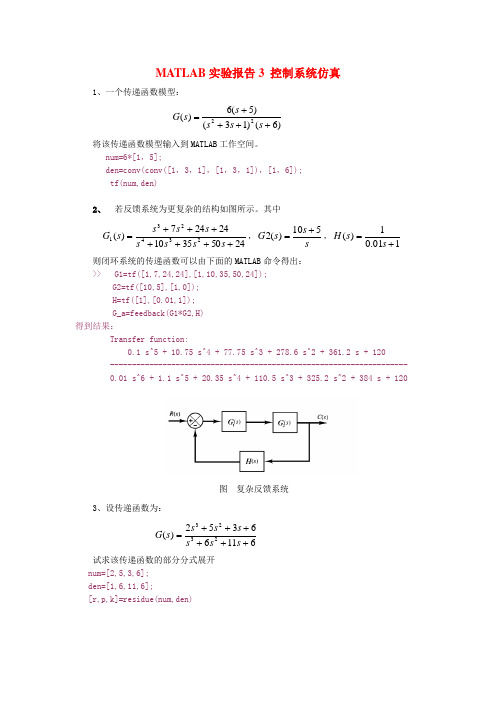
num=6*[1,5];den=conv(conv([1,3,1],[1,3,1]),[1,6]);tf(num,den)2、 若反馈系统为更复杂的结构如图所示。
其中2450351024247)(234231+++++++=s s s s s s s s G ,s s s G 510)(2+=,101.01)(+=s s H 则闭环系统的传递函数可以由下面的MATLAB 命令得出:>> G1=tf([1,7,24,24],[1,10,35,50,24]);G2=tf([10,5],[1,0]);H=tf([1],[0.01,1]);G_a=feedback(G1*G2,H)得到结果:Transfer function:0.1 s^5 + 10.75 s^4 + 77.75 s^3 + 278.6 s^2 + 361.2 s + 120 -------------------------------------------------------------------- 0.01 s^6 + 1.1 s^5 + 20.35 s^4 + 110.5 s^3 + 325.2 s^2 + 384 s + 1203、设传递函数为:61166352)(2323++++++=s s s s s s s G 试求该传递函数的部分分式展开num=[2,5,3,6];den=[1,6,11,6];[r,p,k]=residue(num,den)图 复杂反馈系统4、给定单位负反馈系统的开环传递函数为:)7()1(10)(++=s s s s G 试画出伯德图。
利用以下MATLAB 程序,可以直接在屏幕上绘出伯德图如图20。
>> num=10*[1,1];den=[1,7,0];bode(num,den)5、已知三阶系统开环传递函数为:)232(27)(23+++=s s s s G画出系统的奈氏图,求出相应的幅值裕量和相位裕量,并求出闭环单位阶跃响应曲线。
MATLAB与控制系统仿真及实验 2016 (五)
MATLAB与控制系统仿真及实验实验报告(五)2015- 2016 学年第 2 学期专业:班级:学号:姓名:20 年月日实验五 SIMULINK系统仿真设计一、实验目的1、掌握SIMULINK工作环境及特点2、掌握线性系统仿真常用的基本模块的用法3、掌握SIMULINK的建模与仿真方法4、子系统的创建和封装设计二、实验设备及条件计算机一台(包含MATLAB 软件环境)。
三、实验原理四、实验内容1. 建立单位负反馈二阶系统的SIMULINK仿真模型,当输入信号源分别为阶跃信号、斜坡信号、正弦信号时,给出系统输出的波形图。
开环传递函数如下所示2. 利用SIMULINK 仿真下列曲线并给出结果,取πω2=,tt t t t t x ωωωωωω9sin 917sin 715sin 513sin 31sin )(++++=3. 先建立一个子系统,再利用该子系统产生曲线2sin(2)xy e x -=π。
4. 建立一个PID 控制器的SIMULINK 模型,将其封装。
已知单位负反馈控制系统的传递函数为错误!未找到引用源。
要求在单位阶跃信号作用下绘制其相应曲线,并使用P ,PI ,PD 和PID 控制器分别改善其性能。
Kp=0.5Kp=0.5 Ki=1/60Kp=0.5 Kd=0.3Kp=1 Ki=1/60 Kd=0.3五、心得体会通过这次实验掌握了SIMULINK工作环境及特点,掌握了线性系统仿真常用的基本模块的用法,掌握了SIMULINK的建模与仿真方法,学会了子系统的创建和封装设计。
实验开始是对于PID控制器的使用好不够熟练,实验做完后已经可以熟练使用。
《MATLAB与控制系统仿真》实验报告

《MATLAB与控制系统仿真》实验报告一、实验目的本实验旨在通过MATLAB软件进行控制系统的仿真,并通过仿真结果分析控制系统的性能。
二、实验器材1.计算机2.MATLAB软件三、实验内容1.搭建控制系统模型在MATLAB软件中,通过使用控制系统工具箱,我们可以搭建不同类型的控制系统模型。
本实验中我们选择了一个简单的比例控制系统模型。
2.设定输入信号我们需要为控制系统提供输入信号进行仿真。
在MATLAB中,我们可以使用信号工具箱来产生不同类型的信号。
本实验中,我们选择了一个阶跃信号作为输入信号。
3.运行仿真通过设置模型参数、输入信号以及仿真时间等相关参数后,我们可以运行仿真。
MATLAB会根据系统模型和输入信号产生输出信号,并显示在仿真界面上。
4.分析控制系统性能根据仿真结果,我们可以对控制系统的性能进行分析。
常见的性能指标包括系统的稳态误差、超调量、响应时间等。
四、实验步骤1. 打开MATLAB软件,并在命令窗口中输入“controlSystemDesigner”命令,打开控制系统工具箱。
2.在控制系统工具箱中选择比例控制器模型,并设置相应的增益参数。
3.在信号工具箱中选择阶跃信号,并设置相应的幅值和起始时间。
4.在仿真界面中设置仿真时间,并点击运行按钮,开始仿真。
5.根据仿真结果,分析控制系统的性能指标,并记录下相应的数值,并根据数值进行分析和讨论。
五、实验结果与分析根据运行仿真获得的结果,我们可以得到控制系统的输出信号曲线。
通过观察输出信号的稳态值、超调量、响应时间等性能指标,我们可以对控制系统的性能进行分析和评价。
六、实验总结通过本次实验,我们学习了如何使用MATLAB软件进行控制系统仿真,并提取控制系统的性能指标。
通过实验,我们可以更加直观地理解控制系统的工作原理,为控制系统设计和分析提供了重要的工具和思路。
七、实验心得通过本次实验,我深刻理解了控制系统仿真的重要性和必要性。
MATLAB软件提供了强大的仿真工具和功能,能够帮助我们更好地理解和分析控制系统的性能。
MATLAB仿真实验实验内容(2016)_32457
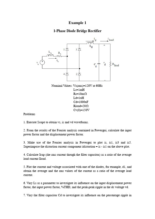
Example 11-Phase Diode Bridge RectifierNominal Values: Vs(rms)=120V at 60HzLs=1mHRs=10mΩLd=1uHCd=1000uFRload=20ΩCv(0)=150VProblems1. Execute Scope to obtain vs, is and vd waveforms.2. From the results of the Fourier analysis contained in Powergui, calculate the input power factor and the displacement power factor.3. Make use of the Fourier analysis in Powergui to plot is, is1, is3 and is5. Superimpose the distortion current component idistortion = is - is1 on the above plot.4. Calculate Icap (the rms current though the filter capacitor) as a ratio of the average load current Iload.5. Plot the current and voltage associated with one of the diodes, for example, d1, and obtain the average and the rms values of the current as a ratio of the average load current.6. Vary Ls as a parameter to investigate its influence on the input displacement power factor, the input power factor, %THD, and the peak-peak ripple in the dc voltage vd.7. Vary the filter capacitor Cd to investigate its influence on the percentage ripple invd, input displacement power factor and %THD. Plot the percentage ΔVd (peak-to-peak) / Vd (average) as a function of Cd.8. Vary the load power to investigate its influence on the average dc voltage.9. Obtain the vs, is and vd waveforms during the startup transient when the filter capacitor is initially not charged. Obtain the peak inrush current as a ratio of the peak current in steady state. Vary the switching instant by simply varying the phase angle θof the source vs. (Hint: change Cv(0)=150V to Cv(0)=0V)10. Replace the dc side of the diode bridge by a current source I d=10A, corresponding to a very large Ld . Make Ls almost equal to zero. Obtain Vd(average).11.Make Ls=3 mH in Problem 9 and obtain Vd (average), displacement power factor, power factor, %THD.Example 23-Phase Diode Bridge RectifierNominal Values: V LL(rms)=208V at 60HzLs=0.1mHRs=1mΩLd=0.5mHRd=5mΩCd=500uFRload=16.5ΩProblems:1. (a)Obtain v ab, v d and i d waveforms.(b)Obtain v a and i a waveforms2. By means of Fourier analysis of ia, calculate its harmonic components as a ratio of Ia1.3. Calculate Ia, Ia1, Idis, %THD in the input current, input displacement power factor and the input power factor. How do the results compare with the 1-phase diode-bridge rectifier of Example 1.4. Calculate Icap(the rms current through the filter capacitor) as a ratio of the average load current Iload. Compare the results with that in Example 1.5. Investigate the influence of Ld on the input displacement power factor, the input power factor and the average dc voltage Vd. Suggested range of Ld: 0.1 mH to 10 mH.6. Investigate the influence of Cd on the percent ripple in vd. Plot the percentage ΔVd(peak-to-peak)/Vd(average) as a function of Cd. Suggested range of Cd: 100uF and 2,000uF.7. Investigate the influence of Cd on the input displacement power factor and the input power factor. Suggested range of Cd: 100μF to 2,000μF.8. Plot the average dc voltage as a function of load. Suggested range of R load: 50Ω to 8Ω.Example 53-Phase Thyristor Rectifier BridgeNominal Values: V LL (rms)=208V at 60HzLs1=0.2mHLs2=1mHLd=16mHRload=16.5Ωdelay angle=45°Problems1. (a) Obtain va, vd and id waveforms using Scope.(b) Obtain va and ia waveforms.(c) Obtain (va)pcc, (vab)pcc and ia waveforms.2. From the plots, obtain the commutation interval u and id at the start of the commutation. Verify the following commutation equation:2cos()cos 2s d LL L u I V ωαα+=−where Ls = Ls1 + Ls2. For Id, use the average value of id or its value at the start of the commutation.3. By means of Fourier analysis of is, calculate its harmonic components as a ratio of Is1.4. Calculate Is, %THD in the input current, the input displacement power factor and the input power factor.5. Verify the following equation:Displacement power factor cos cos()cos()22uu ααα++≅+≅6. At the point of common coupling, obtain the following from the voltage v pccwaveform:(a) Line-notch depth ρ(%)(b) Line-notch area and,(c) voltage THD%.7. Obtain the average dc voltage Vd. Verify that31.35cos sd LL d L V V I ωαπ=−For Id, use the average value of id or its value at the start of the commutation.3-Phase Thyristor InverterNominal Values: V LL(rms)=480V at 60HzLs=0.1mHLd=16mHRd=1ΩE=480Vdelay angle α=160°Problems:1. (a) Obtain va , vd and id waveforms using scope.(b) Obtain va and ia waveforms2. Calculate Is, %THD in the input current, the input displacement power factor and the input power factor.3. Study the startup of the inverter operation. Increase the delay angle to a value close to 180° and look at the va, vd and id waveforms. Repeat the above procedure by reducing αslowly to its nominal value of 160°. Plot the average dc current Id versus α.Step-down (BUCK) dc-dc ConverterNominal Values: V d =8V(dc)L=5uHrL=10m ΩC=100uFRload=0.5Ωfs=100kHzswitch duty ratio D=0.75Problems1. In steady state, obtain the following waveforms using Scope:(a) vL and iL waveforms.(b) vo, iL and ic waveforms2. Obtain voi waveform and by means of Fourier analysis, obtain its harmonic components as a ratio of its average value V o.3. Increase the load resistance to 10Ω. Obtain vL and iL waveforms in the discontinuous conduction mode [Hint: use V(0)=5.8V and I L (0)=0]. Check if the results agree with the following equation:22,max 1()4o o d LB V D I V D I =+ Where ,max 8d LB sV I Lf = . 4. Obtain the peak-to-peak ripple in the output voltage and check to see if the results agree with the analytical calculations.5. Calculate the rms value of the current through the output capacitor as a ratio of theaverage load current Io.6. Calculate the peak-to-peak ripple in the output voltage in the presence of the output capacitor Equivalent Series Resistance (ESR)[Suggested ESR=100mΩ]. Plot the ripple across C, ESR and the total ripple in vo.Example 10Full-Bridge, Bipolar-Switching dc-dc ConverterNominal Values: V d=200VV EMF=79.5VRa=0.37ΩLa=1.5mHIo(avg)=10Afs=20kHzswitch duty ratio D1 of T A1 and T B2=0.708(so v control=0.416V with Vtri=1.0V)Problems:1. Obtain the following waveforms using Scope:(a) vo, io and po(t) = vo*io(b) vo and id2. Calculate peak-to-peak ripple in io.3. By means of Fourier analysis, calculate the average value and the harmonic components in vo. Obtain the rms value of the ripple in vo and check it with theanalytical calculations.4. By means of Fourier analysis, calculate the average value of id and the rms value ofthe ripple.5. With V EMF=0 and Ia(avg)=0, V o(avg)=0V. Therefore, Vcontrol=0. Calculate thefollowing [Hint: use Io(0)=-1.67A]:(a) vo, ioand po(t) waveforms.(b) peak-to-peak ripple in io. Compare it with its analytical value, and that in Problem 2.(c) In part (a), label the intervals during which various devices are conducting.6. In the regenerative mode, the power flows from the load to the dc-bus at Vd. Let V EMF =79.5V , Ia(avg)=10A in the reverse direction, and V o(avg)=79.5-0.37×10=75.8V . Therefore,75.8 1.00.379200control V =×= Calculate parts (a) through (c) of Problem 5 [Hint: use Io(0)=-11.67 A].Example 121-Phase, Bipolar-Voltage Switching InverterNominal Values: Frequency f1=40Hz, V o1(rms)=153.33V, V o1(peak)=216.8V.R TH=2Ω, L TH=10mH. Io1(rms)=10A at a 0.866 pf (lagging)Therefore, V TH(rms)=124.1 5.39∠−°Vand v TH=175.5sin(2π*40t-5.39°).Inverter and Controller for Sinusoidal PWM:Switching frequency fs=1kHz,Frequency modulation ratio m f=1000/40=25;Amplitude modulation ratio m a=0.8.Therefore, Vd=Vo1, peak/m a=271 V and,v control=0.8sin(2π*40t).Problems:1. Obtain the following waveforms using Scope:(a) vo and io.(b) vo and id.(c) vo, io and po.2. Obtain vo1 by means of Fourier analysis of the vo waveform. Compare vo1 with its precalculated nominal value.3. Using the results of Problem 2, obtain the ripple component v,ripple waveform in the output voltage.4. Obtain io1 by means of Fourier analysis of the io waveform. Compare io1 with its precalculated nominal value.5. Using the results of Problem 4, obtain the ripple component i,ripple in the output current.6. Obtain Id(avg) and id2 (the component at the 2nd harmonic frequency) by means of the Fourier analysis of the id waveform. Compare them with their precalculated nominal values.ing the results of Problem 6, obtain the high frequency ripple componentid,ripple in the input dc current. Calculate its rms value.Based on Io1(rms)=1030∠o A, the initial value Io(0)=-7A.-Example 16Three-Phase PWM InverterNominal Values:Load: A 230V ,60Hz, 3-phase motor is operating at a frequency f 1=47.619Hz. Therefore,147.619230182.54V 60rms LL V =×= 11105.39V=105.3903rms LL rmsAn V V ==∠°110A rms A I =at a lagging power factor of 0.8661030A =∠−° Rs=2Ω, Ls=10mH,Xs=3247.61910103π−×××=Ω(V TH ,A )1=74.7612.36V(rms)∠−°Inverter and Controller for Sinusoidal PWM:Switching frequency fs=1kHz,Amplitude modulation ratio m a =0.95. 1313.97V 0.612rms LL d aV V m ==.With Vtri=1.0V v control, A =0.95cos(2πf 1t-90°)V .Problems :1. Obtain the following waveforms using :(a) v AN and i A .(b) v an and i A .(c) v AN and id.2. Obtain vAn1 by means of Fourier analysis of the vAn waveform. Compare vAn1 with its precalculated nominal value.3. Using the results of Problem 2, obtain the ripple component v,ripple waveform in the output voltage.4. Obtain iA1 by means of Fourier analysis of iA waveform. Compare iA1 with its precalculated nominal value.5. Using the results of Problem 4, obtain the ripple component i,ripple in the output current.6. Obtain Id(avg) by means of Fourier analysis and obtain the high frequency ripple id,ripple = id - Id(avg) in the input current.7. Obtain the load neutral voltage with respect to the mid-point of the dc input voltage.Based on IA1(rms)=1030-∠o A, the initial value IA1(0)=-7.07A.。
matlab的控制系统仿真与应用 第五章

[ n a n , n1 a n1 ,,1 a1 ] T 1
a n 2 a1 a n 3 1 0 1 0 0
a n 1 a n2 T b A b A n 1 b a1 1 函数bass_pp( ) 调用格式为:
1
2 n K v1 v2 vn
n v1 v2 vn
1
i K ,于是 vi
vi V,对于给定 i ,可以求出 i i
vi
一般说来
v1
v2 v n 可逆,否则重新选择 1 2 n 。
n V1 1 V2 2 Vn n
ai
(i=1,2,…,n - 1)为特征多项式系数,即
sI a s n a1 s n 1 an 1 s an 0
定义新的状态
ˆ x
x=T
ˆ x
1.变换法
由于系统可控,因此T可逆,系统变换成
1 1 ˆ T aTx ˆ T bu x
其中
0 0 1 T aT 0 an 1 0 0 an 1 0 1 0 a n 2 0 0 0 0 1 T b 1 0 a1 1
若假定 i 与A的特征值有相同的,或 i 中有重根时, i 1,2,, n 则可以对特征值相同的一个或几个加上一定的微小偏量,使之满足上面第一种 情形的条件。然后,再重新进行极点配置。如果效果不够理想,那么还可重新选择 1 2 n 阵来进行配置。 控制系统工具箱中place( )函数是基于鲁棒极点配置的算法,用来求取状态反馈 阵K,使得多输入系统具有指定的闭环极点P,即 p eig( A B * K ) 。 place( )函数调用格式为:
实验五 控制系统CAD综合实验 控制系统的matlab仿真与设计 王海英 高等教育出版社

实验五 控制系统CAD 综合实验实验题目1. (1)试编写m 文件,绘制零初始条件下下列系统的单位阶跃响应曲线。
具体要求。
a) K=1,T=[0.001:0.1:4]秒;b) T=0.5秒,K=[0.5:1:20]。
(2) 构建下列系统的simulink 模型,并对虚线内的子系统进行封装,讨论采样周期和开环增益对系统稳定性的影响。
(1)m 文件如下:%5-1-1 K=1;hold onfor T=0.001:0.1:4G0=tf(K,conv([1,0],[1,1])); G0=c2d(G0,T); G1=feedback(G0,1); step(G1); end hold off figure hold on T=0.5;for K=0.5:1:20G0=tf(K,conv([1,0],[1,1])); G0=c2d(G0,T);G1=feedback(G0,1); step(G1); endR(s)C(s)执行结果:(2)simulink模型:执行结果:2.已知含有非线性环节的控制系统如图所示。
完成下列仿真。
a b c(1)非线性环节特性如图a所示。
通过编写m文件,仿真对比非线性环节对系统特性的影响(稳定性,暂态以及稳态三方面),绘制有无非线性环节两种条件下系统单位阶跃响应曲线。
参考教材p285。
(2)非线性环节特性如图b所示。
通过仿真对比非线性环节参数m与h对系统特性的影响(稳定性,暂态以及稳态三方面)。
当m=1,h=0.5时,绘制零初始条件下,该系统单位阶跃响应的相轨迹图。
(3)非线性环节特性如图c所示。
通过仿真对比非线性环节参数h对系统特性的影响(稳定性,暂态以及稳态三方面)。
当h=0.5时,绘制系统初始条件)0(c,3)0(c== 时该系统的相轨迹图。
(1)m文件:G0=tf(conv(20,[1,0.5]),conv([1,0],conv([1,0.1],conv([1,2],[1,10]))));Gb1=feedback(G0,1);[y1,t1]=step(Gb1);e2(2)=1;y(1)=0;t(1)=0;uc(1)=1;s1=0.6;for n=3:300if e2(n-1)<=-s1uc(n-1)=e2(n-1)+s1;elseif e2(n-1)>=s1uc(n-1)=e2(n-1)-s1;elseuc(n-1)=0;endt(n-1)=0.1*(n-2);[y,nu]=lsim(G0,uc,t);e2(n)=1.-y(n-1); endplot(t,y);Simulink仿真:有无非线性环节两种条件下系统单位阶跃响应曲线(2)Simulink仿真:5-2-2.mdlMatlab命令:[t,x,y]=sim('5-2-2',10,[],[]);plot(y(:,1),y(:,2));5相轨迹图(3)Simulink仿真:仿真对比非线性环节参数h对系统特性的影响:Matlab命令:[t,x,y]=sim('T5_2_c2',100,[],[]);plot(y(:,1),y(:,2));初始条件0= 时该系统的相轨迹图)0(c,3)0(c=。
《MATLAB与控制系统仿真》实验报告
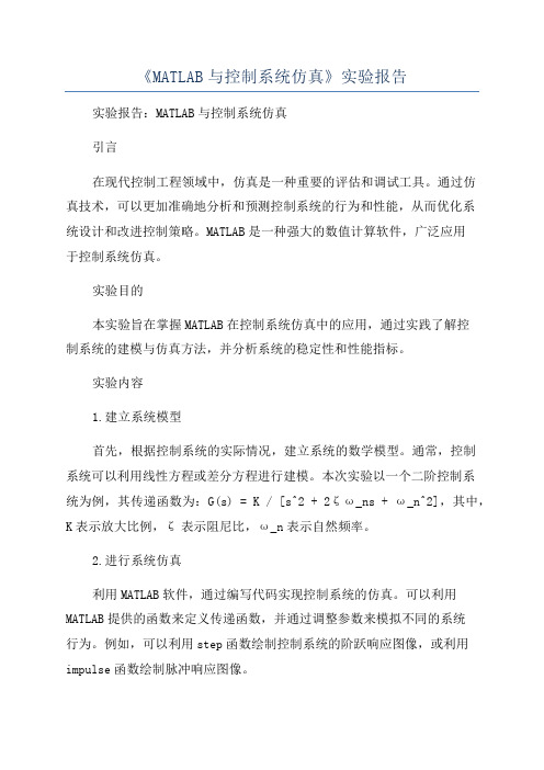
《MATLAB与控制系统仿真》实验报告实验报告:MATLAB与控制系统仿真引言在现代控制工程领域中,仿真是一种重要的评估和调试工具。
通过仿真技术,可以更加准确地分析和预测控制系统的行为和性能,从而优化系统设计和改进控制策略。
MATLAB是一种强大的数值计算软件,广泛应用于控制系统仿真。
实验目的本实验旨在掌握MATLAB在控制系统仿真中的应用,通过实践了解控制系统的建模与仿真方法,并分析系统的稳定性和性能指标。
实验内容1.建立系统模型首先,根据控制系统的实际情况,建立系统的数学模型。
通常,控制系统可以利用线性方程或差分方程进行建模。
本次实验以一个二阶控制系统为例,其传递函数为:G(s) = K / [s^2 + 2ζω_ns + ω_n^2],其中,K表示放大比例,ζ表示阻尼比,ω_n表示自然频率。
2.进行系统仿真利用MATLAB软件,通过编写代码实现控制系统的仿真。
可以利用MATLAB提供的函数来定义传递函数,并通过调整参数来模拟不同的系统行为。
例如,可以利用step函数绘制控制系统的阶跃响应图像,或利用impulse函数绘制脉冲响应图像。
3.分析系统的稳定性与性能在仿真过程中,可以通过调整控制系统的参数来分析系统的稳定性和性能。
例如,可以改变放大比例K来观察系统的超调量和调整时间的变化。
通过观察控制系统的响应曲线,可以判断系统的稳定性,并计算出性能指标,如超调量、调整时间和稳态误差等。
实验结果与分析通过MATLAB的仿真,我们得到了控制系统的阶跃响应图像和脉冲响应图像。
通过观察阶跃响应曲线,我们可以得到控制系统的超调量和调整时间。
通过改变放大比例K的值,我们可以观察到超调量的变化趋势。
同时,通过观察脉冲响应曲线,我们还可以得到控制系统的稳态误差,并判断系统的稳定性。
根据实验结果分析,我们可以得出以下结论:1.控制系统的超调量随着放大比例K的增大而增大,但当K超过一定值后,超调量开始减小。
2.控制系统的调整时间随着放大比例K的增大而减小,即系统的响应速度加快。
MATLAB仿真实验实验内容(2016)_32457

Example 11-Phase Diode Bridge RectifierNominal Values: Vs(rms)=120V at 60HzLs=1mHRs=10mΩLd=1uHCd=1000uFRload=20ΩCv(0)=150VProblems1. Execute Scope to obtain vs, is and vd waveforms.2. From the results of the Fourier analysis contained in Powergui, calculate the input power factor and the displacement power factor.3. Make use of the Fourier analysis in Powergui to plot is, is1, is3 and is5. Superimpose the distortion current component idistortion = is - is1 on the above plot.4. Calculate Icap (the rms current though the filter capacitor) as a ratio of the average load current Iload.5. Plot the current and voltage associated with one of the diodes, for example, d1, and obtain the average and the rms values of the current as a ratio of the average load current.6. Vary Ls as a parameter to investigate its influence on the input displacement power factor, the input power factor, %THD, and the peak-peak ripple in the dc voltage vd.7. Vary the filter capacitor Cd to investigate its influence on the percentage ripple invd, input displacement power factor and %THD. Plot the percentage ΔVd (peak-to-peak) / Vd (average) as a function of Cd.8. Vary the load power to investigate its influence on the average dc voltage.9. Obtain the vs, is and vd waveforms during the startup transient when the filter capacitor is initially not charged. Obtain the peak inrush current as a ratio of the peak current in steady state. Vary the switching instant by simply varying the phase angle θof the source vs. (Hint: change Cv(0)=150V to Cv(0)=0V)10. Replace the dc side of the diode bridge by a current source I d=10A, corresponding to a very large Ld . Make Ls almost equal to zero. Obtain Vd(average).11.Make Ls=3 mH in Problem 9 and obtain Vd (average), displacement power factor, power factor, %THD.Example 23-Phase Diode Bridge RectifierNominal Values: V LL(rms)=208V at 60HzLs=0.1mHRs=1mΩLd=0.5mHRd=5mΩCd=500uFRload=16.5ΩProblems:1. (a)Obtain v ab, v d and i d waveforms.(b)Obtain v a and i a waveforms2. By means of Fourier analysis of ia, calculate its harmonic components as a ratio of Ia1.3. Calculate Ia, Ia1, Idis, %THD in the input current, input displacement power factor and the input power factor. How do the results compare with the 1-phase diode-bridge rectifier of Example 1.4. Calculate Icap(the rms current through the filter capacitor) as a ratio of the average load current Iload. Compare the results with that in Example 1.5. Investigate the influence of Ld on the input displacement power factor, the input power factor and the average dc voltage Vd. Suggested range of Ld: 0.1 mH to 10 mH.6. Investigate the influence of Cd on the percent ripple in vd. Plot the percentage ΔVd(peak-to-peak)/Vd(average) as a function of Cd. Suggested range of Cd: 100uF and 2,000uF.7. Investigate the influence of Cd on the input displacement power factor and the input power factor. Suggested range of Cd: 100μF to 2,000μF.8. Plot the average dc voltage as a function of load. Suggested range of R load: 50Ω to 8Ω.Example 53-Phase Thyristor Rectifier BridgeNominal Values: V LL (rms)=208V at 60HzLs1=0.2mHLs2=1mHLd=16mHRload=16.5Ωdelay angle=45°Problems1. (a) Obtain va, vd and id waveforms using Scope.(b) Obtain va and ia waveforms.(c) Obtain (va)pcc, (vab)pcc and ia waveforms.2. From the plots, obtain the commutation interval u and id at the start of the commutation. Verify the following commutation equation:2cos()cos 2s d LL L u I V ωαα+=−where Ls = Ls1 + Ls2. For Id, use the average value of id or its value at the start of the commutation.3. By means of Fourier analysis of is, calculate its harmonic components as a ratio of Is1.4. Calculate Is, %THD in the input current, the input displacement power factor and the input power factor.5. Verify the following equation:Displacement power factor cos cos()cos()22uu ααα++≅+≅6. At the point of common coupling, obtain the following from the voltage v pccwaveform:(a) Line-notch depth ρ(%)(b) Line-notch area and,(c) voltage THD%.7. Obtain the average dc voltage Vd. Verify that31.35cos sd LL d L V V I ωαπ=−For Id, use the average value of id or its value at the start of the commutation.3-Phase Thyristor InverterNominal Values: V LL(rms)=480V at 60HzLs=0.1mHLd=16mHRd=1ΩE=480Vdelay angle α=160°Problems:1. (a) Obtain va , vd and id waveforms using scope.(b) Obtain va and ia waveforms2. Calculate Is, %THD in the input current, the input displacement power factor and the input power factor.3. Study the startup of the inverter operation. Increase the delay angle to a value close to 180° and look at the va, vd and id waveforms. Repeat the above procedure by reducing αslowly to its nominal value of 160°. Plot the average dc current Id versus α.Step-down (BUCK) dc-dc ConverterNominal Values: V d =8V(dc)L=5uHrL=10m ΩC=100uFRload=0.5Ωfs=100kHzswitch duty ratio D=0.75Problems1. In steady state, obtain the following waveforms using Scope:(a) vL and iL waveforms.(b) vo, iL and ic waveforms2. Obtain voi waveform and by means of Fourier analysis, obtain its harmonic components as a ratio of its average value V o.3. Increase the load resistance to 10Ω. Obtain vL and iL waveforms in the discontinuous conduction mode [Hint: use V(0)=5.8V and I L (0)=0]. Check if the results agree with the following equation:22,max 1()4o o d LB V D I V D I =+ Where ,max 8d LB sV I Lf = . 4. Obtain the peak-to-peak ripple in the output voltage and check to see if the results agree with the analytical calculations.5. Calculate the rms value of the current through the output capacitor as a ratio of theaverage load current Io.6. Calculate the peak-to-peak ripple in the output voltage in the presence of the output capacitor Equivalent Series Resistance (ESR)[Suggested ESR=100mΩ]. Plot the ripple across C, ESR and the total ripple in vo.Example 10Full-Bridge, Bipolar-Switching dc-dc ConverterNominal Values: V d=200VV EMF=79.5VRa=0.37ΩLa=1.5mHIo(avg)=10Afs=20kHzswitch duty ratio D1 of T A1 and T B2=0.708(so v control=0.416V with Vtri=1.0V)Problems:1. Obtain the following waveforms using Scope:(a) vo, io and po(t) = vo*io(b) vo and id2. Calculate peak-to-peak ripple in io.3. By means of Fourier analysis, calculate the average value and the harmonic components in vo. Obtain the rms value of the ripple in vo and check it with theanalytical calculations.4. By means of Fourier analysis, calculate the average value of id and the rms value ofthe ripple.5. With V EMF=0 and Ia(avg)=0, V o(avg)=0V. Therefore, Vcontrol=0. Calculate thefollowing [Hint: use Io(0)=-1.67A]:(a) vo, ioand po(t) waveforms.(b) peak-to-peak ripple in io. Compare it with its analytical value, and that in Problem 2.(c) In part (a), label the intervals during which various devices are conducting.6. In the regenerative mode, the power flows from the load to the dc-bus at Vd. Let V EMF =79.5V , Ia(avg)=10A in the reverse direction, and V o(avg)=79.5-0.37×10=75.8V . Therefore,75.8 1.00.379200control V =×= Calculate parts (a) through (c) of Problem 5 [Hint: use Io(0)=-11.67 A].Example 121-Phase, Bipolar-Voltage Switching InverterNominal Values: Frequency f1=40Hz, V o1(rms)=153.33V, V o1(peak)=216.8V.R TH=2Ω, L TH=10mH. Io1(rms)=10A at a 0.866 pf (lagging)Therefore, V TH(rms)=124.1 5.39∠−°Vand v TH=175.5sin(2π*40t-5.39°).Inverter and Controller for Sinusoidal PWM:Switching frequency fs=1kHz,Frequency modulation ratio m f=1000/40=25;Amplitude modulation ratio m a=0.8.Therefore, Vd=Vo1, peak/m a=271 V and,v control=0.8sin(2π*40t).Problems:1. Obtain the following waveforms using Scope:(a) vo and io.(b) vo and id.(c) vo, io and po.2. Obtain vo1 by means of Fourier analysis of the vo waveform. Compare vo1 with its precalculated nominal value.3. Using the results of Problem 2, obtain the ripple component v,ripple waveform in the output voltage.4. Obtain io1 by means of Fourier analysis of the io waveform. Compare io1 with its precalculated nominal value.5. Using the results of Problem 4, obtain the ripple component i,ripple in the output current.6. Obtain Id(avg) and id2 (the component at the 2nd harmonic frequency) by means of the Fourier analysis of the id waveform. Compare them with their precalculated nominal values.ing the results of Problem 6, obtain the high frequency ripple componentid,ripple in the input dc current. Calculate its rms value.Based on Io1(rms)=1030∠o A, the initial value Io(0)=-7A.-Example 16Three-Phase PWM InverterNominal Values:Load: A 230V ,60Hz, 3-phase motor is operating at a frequency f 1=47.619Hz. Therefore,147.619230182.54V 60rms LL V =×= 11105.39V=105.3903rms LL rmsAn V V ==∠°110A rms A I =at a lagging power factor of 0.8661030A =∠−° Rs=2Ω, Ls=10mH,Xs=3247.61910103π−×××=Ω(V TH ,A )1=74.7612.36V(rms)∠−°Inverter and Controller for Sinusoidal PWM:Switching frequency fs=1kHz,Amplitude modulation ratio m a =0.95. 1313.97V 0.612rms LL d aV V m ==.With Vtri=1.0V v control, A =0.95cos(2πf 1t-90°)V .Problems :1. Obtain the following waveforms using :(a) v AN and i A .(b) v an and i A .(c) v AN and id.2. Obtain vAn1 by means of Fourier analysis of the vAn waveform. Compare vAn1 with its precalculated nominal value.3. Using the results of Problem 2, obtain the ripple component v,ripple waveform in the output voltage.4. Obtain iA1 by means of Fourier analysis of iA waveform. Compare iA1 with its precalculated nominal value.5. Using the results of Problem 4, obtain the ripple component i,ripple in the output current.6. Obtain Id(avg) by means of Fourier analysis and obtain the high frequency ripple id,ripple = id - Id(avg) in the input current.7. Obtain the load neutral voltage with respect to the mid-point of the dc input voltage.Based on IA1(rms)=1030-∠o A, the initial value IA1(0)=-7.07A.。
《MATLAB仿真技术》实验指导书2016附问题详解
实验项目及学时安排实验一 MATLAB环境的熟悉与基本运算 2学时实验二 MATLAB数值计算实验 2学时实验三 MATLAB数组应用实验 2学时实验四 MATLAB符号计算实验 2学时实验五 MATLAB的图形绘制实验 2学时实验六 MATLAB的程序设计实验 2学时实验七 MATLAB工具箱Simulink的应用实验 2学时实验八 MATLAB图形用户接口GUI的应用实验 2学时实验一 MATLAB环境的熟悉与基本运算一、实验目的1.熟悉MATLAB开发环境2.掌握矩阵、变量、表达式的各种基本运算二、实验基本知识1.熟悉MATLAB环境:MATLAB桌面和命令窗口、命令历史窗口、帮助信息浏览器、工作空间浏览器、文件和搜索路径浏览器。
2.掌握MATLAB常用命令3.MATLAB变量与运算符变量命名规则如下:(1)变量名可以由英语字母、数字和下划线组成(2)变量名应以英文字母开头(3)长度不大于31个(4)区分大小写MATLAB中设置了一些特殊的变量与常量,列于下表。
MATLAB运算符,通过下面几个表来说明MATLAB的各种常用运算符4.MATLAB的一维、二维数组的寻访表6 子数组访问与赋值常用的相关指令格式5.MATLAB的基本运算表7 两种运算指令形式和实质涵的异同表6.MATLAB的常用函数表8 标准数组生成函数表9 数组操作函数三、实验容1、学习使用help命令,例如在命令窗口输入help eye,然后根据帮助说明,学习使用指令eye(其它不会用的指令,依照此方法类推)2、学习使用clc、clear,观察command window、command history和workspace等窗口的变化结果。
3、初步程序的编写练习,新建M-file,保存(自己设定文件名,例如exerc1、exerc2、 exerc3……),学习使用MATLAB的基本运算符、数组寻访指令、标准数组生成函数和数组操作函数。
控制系统计算机仿真(matlab)实验五实验报告
实验五 控制系统计算机辅助设计一、实验目的学习借助MATLAB 软件进行控制系统计算机辅助设计的基本方法,具体包括超前校正器的设计,滞后校正器的设计、滞后-超前校正器的设计方法。
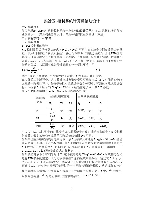
二、实验学时:4 学时 三、实验原理1、PID 控制器的设计PID 控制器的数学模型如公式(5-1)、(5-2)所示,它的三个特征参数是比例系数、积分时间常数(或积分系数)、微分时间常数(或微分系数),因此PID 控制器的设计就是确定PID 控制器的三个参数:比例系数、积分时间常数、微分时间常数。
Ziegler (齐格勒)和Nichols (尼克尔斯)于1942提出了PID 参数的经验整定公式。
其适用对象为带纯延迟的一节惯性环节,即:s e Ts Ks G τ-+=1)( 5-1式中,K 为比例系数、T 为惯性时间常数、τ为纯延迟时间常数。
在实际的工业过程中,大多数被控对象数学模型可近似为式(5-1)所示的带纯延迟的一阶惯性环节。
在获得被控对象的近似数学模型后,可通过时域或频域数据,根据表5-1所示的Ziegler-Nichols 经验整定公式计算PID 参数。
表控制器的参数。
假定某被控对象的单位阶跃响应如图5-4所示。
如果单位阶跃响应曲线看起来近似一条S 形曲线,则可用Ziegler-Nichols 经验整定公式,否则,该公式不适用。
由S 形曲线可获取被控对象数学模型(如公式5-1所示)的比例系数K 、时间常数T 、纯延迟时间τ。
通过表5-1所示的Ziegler-Nichols 经验整定公式进行整定。
如果被控对象不含有纯延迟环节,就不能够通过Ziegler-Nichols 时域整定公式进行PID 参数的整定,此时可求取被控对象的频域响应数据,通过表5-1 所示的Ziegler-Nichols 频域整定公式设计PID 参数。
如果被控对象含有纯延迟环节,可通过pade 命令将纯延迟环节近似为一个四阶传递函数模型,然后求取被控对象的频域响应数据,应用表5-1求取PID 控制器的参数。
控制系统仿真与工具(matlab)实验指导书精选全文

可编辑修改精选全文完整版控制系统仿真与工具实验指导书目录实验一熟悉MATLAB语言工作环境和特点 (1)实验二图形绘制与修饰 (4)实验三系统的时间响应分析 (8)实验四系统的时间响应分析 (12)实验五SIMULINK仿真基础 (14)实验一熟悉MATLAB语言工作环境和特点一、实验目的通过实验使学生熟悉MA TLAB语言的工作环境,并了解MATLAB语言的特点,掌握其基本语法。
二、实验设备PC机MATLAB应用软件三、实验内容本实验从入门开始,使学生熟悉MA TLAB的工作环境,包括命令窗、图形窗和文字编辑器、工作空间的使用等。
1、命令窗(1)数据的输入打开MATLAB后进入的是MA TLAB的命令窗,命令窗是用户与MATLAB做人机对话的主要环境。
其操作提示符为“》”。
在此提示下可输入各种命令并显示出相应的结果,如键入:x1=sqrt(5),x2=1.35,y=3/x2显示结果为:x1=2.2361x2=1.3500y=2.2222上命令行中两式之间用逗号表示显示结果,若用分号,则只运行而不用显示运行结果。
如键入A=[1,2,3;4,5,6;7,8,9],则显示为说明:●直接输入矩阵时,矩阵元素用空格或逗号分隔,矩阵行用分号相隔,整个矩阵放在方括号中。
注意:标点符号一定要在英文状态下输入。
●在MA TLAB中,不必事先对矩阵维数做任何说明,存储时自动配置。
●指令执行后,A被保存在工作空间中,以备后用。
除非用户用clear指令清除它,或对它重新赋值。
●MATLAB对大小写敏感。
(2)数据的显示在MA TLAB工作空间中显示数值结果时,遵循一定的规则,在缺省的情况下,当结果是整数,MATLAB将它作为整数显示;当结果是实数,MATLAB以小数点后4位的精度近似显示。
如果结果中的有效数字超出了这一范围,MATLAB以类似于计算器的计算方法来显示结果。
也可通过键入适当的MA TLAB命令来选择数值格式来取代缺省格式。
本部《Matlab与控制系统仿真》实验报告

(1)画出调试好的数控机床进给系统的PI速度控制和PID位置控制的Simulink模块图。
(2)比较分析仿真结果。
实验编号:
实验七MATLAB数字控制器设计初步
姓名
指导教师
时间
地点
一、实验目的和要求
二、实验设备及材料
三、实验记录
(1)序列 ,的z变换结果。
(2)离散系统的系统函数 ,求其冲激响应h(k)
clear%清除变量
t =0:0.001:2*pi;
subplot(2,2,1);
polar(t, 1+cos(t))
subplot(2,2,2);
plot(cos(t).^3,sin(t).^3)
subplot(2,2,3);
polar(t,abs(sin(t).*cos(t)))
subplot(2,2,4);
实验编号:
实验五MATLAB控制系统工具箱使用
姓名
指导教师
时间
地点
一、实验目的和要求
二、实验设备及材料
三、实验记录
(1)写出传递函数 的部分展开式
(2)编程构建系统
(3)编程绘制单位负反馈的开环传递函数 的伯德图。
实验编号:
实验六数控机床SIMULINK仿真
姓名
指导教师
时间
地点
一、实验目的和要求
二、实验设备及材料
(3)画出离散系统的系统函数 ,的零极点图
(4)若描述离散系统的差分方程为 ,已知激励 ,初始状态y(-1)=1,y(-2)=0,求系统的零输入响应,零状态响应。
(5)已知 ,通过部分分式展开法求F(z)。
实验编号:
实验八MATLAB数字控制器设计
MATLAB与控制系统仿真及实验 2016(五)
一个 Simulink 仿真模型的基本模块包括信源、信宿以及系统三个部分。其中,信源 可以是常数、正弦波、阶梯波等信号源,信宿可以是示波器、图形记录仪等,系统则 是被研究系统的 SIMULINK 方框图。系统、信源、信宿,可以从 SIMULINK 模块库中 直接获得,也可以根据用户意愿用库中的模块构建而成。
2
2、 连续系统的建模与仿真 连续系统指的是可以用微分方程来描述的系统。用于建模连续系统的模块:
Simulink 模块组中的 Continous、Math 以及 Nonlinear 模块库中。 利用 Simulink 进行系统仿真的步骤如下: (1) 建立系统仿真模型,这包括添加模块、设置模块参数以及进行模块连接等操
作。 (2) 设置仿真参数。 (3) 启动仿真并分析仿真结果。
四、实验内容
1. 建立单位负反馈二阶系统的 SIMULINK 仿真模型,当输入信号源分别为阶跃信号、 斜坡信号、正弦信号时,给出系统输出的波形图。开环传递函数如下所示
3
2. 利用 SIMULINK 仿真下列曲线并给出结果,取 2 ,
MATLAB 与控制系统仿真及实验 实验报告
(五) 2015- 2016 学年第 2 学期
专业: 班级: 学号: 姓名:
2016 年 5 月 18 日
实验五 SIMULINK 系统仿真设计 一、实验目的
MATLAB实验2016

实验一 MATLAB基本运算(五)矩阵的运算运算符:+(加)、-(减)、*(乘)、/(右除)、\(左除)、^(乘方)、’(转置)等;常用函数:det(行列式)、inv(逆矩阵)、rank(秩)、eig(特征值、特征向量)、rref (化矩阵为行最简形)例5:>> A=[2 0 –1;1 3 2]; B=[1 7 –1;4 2 3;2 0 1];>> M = A*B % 矩阵A与B按矩阵运算相乘>> det_B = det(B) % 矩阵A的行列式>> rank_A = rank(A)% 矩阵A的秩>> inv_B = inv(B)% 矩阵B的逆矩阵>> [V,D] = eig(B) % 矩阵B的特征值矩阵V与特征向量构成的矩阵D>> X = A/B % A/B = A*B-1,即XB=A,求X>> Y = B\A % B\A = B-1*A,即BY=A,求Y(六)上机练习1.练习数据和符号的输入方式,将前面的命令在命令窗口中执行通过;2.输入A=[7 1 5;2 5 6;3 1 5],B=[1 1 1; 2 2 2; 3 3 3],在命令窗口中执行下列表达式,掌握其含义:A(2, 3) A(:,2) A(3,:) A(:,1:2:3) A(:,3).*B(:,2) A(:,3)*B(2,:) A*B A.*B A^2 A.^2 B/A B./A 3.输入C=1:2:20,则C(i)表示什么?其中i=1,2,3, (10)>> c=1:2:20>> i=1:10>> c(i)4.查找已创建变量的信息,删除无用的变量;5.创建如下变量:在0-3 均匀的产生10个点值,形成10维向量>> A=linspace(0,3,10))3*3阶单位距阵>> B=eye(3),随机距阵: >> randn(3,3),魔方距阵>> magic(3),全0距阵>> zeros(3,3),全1距阵>> E=ones(3,3),6 求方程组的解⎪⎩⎪⎨⎧=++=++=++6543522222321321321x x x x x x x x x>> A=[1 2 2;2 1 2;3 4 5]; B=[2 5 6]; x=A/B x = 0.3692 0.3231 0.8615实验二 MATLAB 程序设计三、实验内容:1、熟悉MATLAB 程序编辑与设计环境2、用for 循环语句实现求1~100的和。
- 1、下载文档前请自行甄别文档内容的完整性,平台不提供额外的编辑、内容补充、找答案等附加服务。
- 2、"仅部分预览"的文档,不可在线预览部分如存在完整性等问题,可反馈申请退款(可完整预览的文档不适用该条件!)。
- 3、如文档侵犯您的权益,请联系客服反馈,我们会尽快为您处理(人工客服工作时间:9:00-18:30)。
MATLAB与控制系统仿真及实验
实验报告
(五)
2015- 2016 学年第 2 学期
专业:
班级:
学号:
姓名:
2016 年 5 月18日
实验五 SIMULINK系统仿真设计
一、实验目的
1、掌握SIMULINK工作环境及特点
2、掌握线性系统仿真常用的基本模块的用法
3、掌握SIMULINK的建模与仿真方法
4、子系统的创建和封装设计
二、实验设备及条件
计算机一台(包含MATLAB 软件环境)。
三、实验原理
Simulink是MATLAB的重要组成部分,提供建立系统模型、选择仿真参数和数值算法、启动仿真程序对该系统进行仿真、设置不同的输出方式来观察仿真结果等功能。
1、 Simulink的基本模块
Simulink的模块库提供了大量模块。
单击模块库浏览器中Simulink前面的“+”号,将看到Simulink模块库中包含的子模块库,单击所需要的子模块库,在右边的窗口中将看到相应的基本模块,选择所需基本模块,可用鼠标将其拖到模型编辑窗口。
同样,在模块库浏览器左侧的Simulink栏上单击鼠标右键,在弹出的快捷菜单中单击Open the ‘Simulink’ Libray 命令,将打开Simulink基本模块库窗口。
单击其中的子模块库图标,打开子模块库,找到仿真所需要的基本模块。
Simulink中几乎所有模块的参数都允许用户进行设置,只要双击要设置的模块或在模块上按鼠标右键并在弹出的快捷菜单中选择相应模块的参数设置命令就会弹出模块参数对话框。
该对话框分为两部分,上面一部分是模块功能说明,下面一部分用来进行模块参数设置。
同样,先选择要设置的模块,再在模型编辑窗口Edit菜单下选择相应模块的参数设置命令也可以打开模块参数对话框。
一个Simulink仿真模型的基本模块包括信源、信宿以及系统三个部分。
其中,信源可以是常数、正弦波、阶梯波等信号源,信宿可以是示波器、图形记录仪等,系统则是被研究系统的SIMULINK方框图。
系统、信源、信宿,可以从SIMULINK模块库中直接获得,也可以根据用户意愿用库中的模块构建而成。
2、连续系统的建模与仿真
连续系统指的是可以用微分方程来描述的系统。
用于建模连续系统的模块:Simulink模块组中的Continous、Math以及Nonlinear模块库中。
利用Simulink进行系统仿真的步骤如下:
(1) 建立系统仿真模型,这包括添加模块、设置模块参数以及进行模块连接等操作。
(2) 设置仿真参数。
(3) 启动仿真并分析仿真结果。
四、实验内容
1. 建立单位负反馈二阶系统的SIMULINK仿真模型,当输入信号源分别为阶跃信号、
斜坡信号、正弦信号时,给出系统输出的波形图。
开环传递函数如下所示
2. 利用SIMULINK 仿真下列曲线并给出结果,取πω2=,
t
t t t t t x ωωωωωω9sin 91
7sin 715sin 513sin 31sin )(++++=
3. 先建立一个子系统,再利用该子系统产生曲线
2sin(2)x
y e x -=π。
4. 建立一个PID控制器的SIMULINK模型,将其封装。
已知单位负反馈控制系统的传递函数为
要求在单位阶跃信号作用下绘制其相应曲线,并使用P,PI,PD和PID控制器分别改善其性能。
控制器模型如下:
P控制器:
PI: PD:
PID:
5. (附加题) 控制对象为:G
s s s =
++
32
523500
87.3510470
采样时间为1ms,取指令信号
30
d
y=,控制信号界限为[-6,6],分别采用普通PI控制算
法和抗积分饱和算法进行系统的阶跃响应,比较测试结果。
提示:1、积分分离;2、实现积分饱和算法
五、心得体会
这次仿真实验与自控原理相关,让我们实践与理论相结合,深入的实践了控制原理的许多理论,加深了对课程的理解。