Matlab第二、三次上机作业
Matlab编程与应用习题和一些参考答案

Matlab编程与应用习题和一些参考答案Matlab 上机实验一、二3.求下列联立方程的解⎪⎪⎩⎪⎪⎨⎧=+-+-=-+=++-=--+41025695842475412743w z y x w z x w z y x w z y x >> a=[3 4 -7 -12;5 -7 4 2;1 0 8 -5;-6 5 -2 10];>> b=[4;4;9;4];>> c=a\b4.设⎥⎥⎥⎦⎤⎢⎢⎢⎣⎡------=81272956313841A ,⎥⎥⎥⎦⎤⎢⎢⎢⎣⎡-----=793183262345B ,求C1=A*B’;C2=A’*B;C3=A.*B,并求上述所有方阵的逆阵。
>> A=[1 4 8 13;-3 6 -5 -9;2 -7 -12 -8];>> B=[5 4 3 -2;6 -2 3 -8;-1 3 -9 7];>> C1=A*B'>> C2=A'*B>> C3=A.*B>> inv(C1)>> inv(C2)>> inv(C3)5.设 ⎥⎦⎤⎢⎣⎡++=)1(sin 35.0cos 2x x x y ,把x=0~2π间分为101点,画出以x 为横坐标,y 为纵坐标的曲线。
>> x=linspace(0,2*pi,101);>> y=cos(x)*(0.5+(1+x.^2)\3*sin(x));>> plot(x,y,'r')6.产生8×6阶的正态分布随机数矩阵R1, 求其各列的平均值和均方差。
并求该矩阵全体数的平均值和均方差。
(mean var )a=randn(8,6)mean(a)var(a)k=mean(a)k1=mean(k)i=ones(8,6)i1=i*k1i2=a-i1i3=i2.*i2g=mean(i3)g2=mean(g)10.利用帮助查找limit 函数的用法,并自己编写,验证几个函数极限的例子。
Matlab上机作业部分参考答案.ppt

[rank(A), rank([A B])]
ans =
34 由得出的结果看,A, [A;B] 两个矩阵的秩不同,故方程是
矛盾方程,没有解。
5. 试求下面齐次方程的基础解系
7. 建立如下一个元胞数组,现在要求计算第一个元胞第4行第 2列加上第二个元胞+第三个元胞里的第二个元素+最后一个元 胞的第二个元素。
a={pascal(4),'hello';17.3500,7:2:100}
解: >> a={pascal(4),'hello';17.3500,7:2:100} a=
[ 173/34, 151/34]
6. 求解方程组的通解
x1 2x2 4x3 6x4 3x5 2x6 4 2x1 4x2 4x3 5x4 x5 5x6 3
3x1 6x2 2x3 5x5 9x6 1 2x1 3x2 4x4 x6 8
4x2
5x3
2x4
x5
参考答案: (1) >> limit(sym('(tan(x) - sin(x))/(1cos(2*x))')) ans = 0 (2) >> y = sym('x^3 - 2*x^2 + sin(x)'); >> diff(y) ans = 3*x^2-4*x+cos(x) (3) >> f = x*y*log(x+y); >> fx = diff(f,x) fx = y*log(x+y)+x*y/(x+y)
MATLAB上机内容及作业
MATLAB上机内容及作业无约束优化求解函数fminsearch和fminunc求解无约束非线性优化问题的函数有fminsearch 函数、fminunc 函数。
函数fminsearch和fminunc功能相同,但fminunc函数可以得到目标函数在最优解处的梯度和Hessian矩阵值。
无约束优化数学模型为:min f(X) X∈R n求解无约束非线性优化问题的步骤为:第一步:先编写目标函数的M文件;第二步:再在命令窗口中调用相应的优化函数。
1、fminsearch函数调用格式为[x, fval]=fminsearch(@myfun, x0)输出参数的含义:x:返回最优解的设计变量的值;fval:在最优设计变量值时,目标函数的最小值;exitflag:返回算法终止的标志,有以下几种情况,>0 表示算法收敛于最优解处;=0 表示算法已经达到迭代的最大次数;<0 表示算法不收敛。
output:返回优化算法信息的一个数据结构,有以下信息:output.iteration 表示迭代次数output.algorithm 表示所采用的算法output.funcCount 表示函数评价次数输入参数的含义:@myfun:目标函数的M文件,在其前要加“@”,或表示为'myfun' ,myfun自己可以任意命名;x0:在调用该优化函数时,需要先对设计变量赋一个初始值;2、fminunc函数的调用格式[x, fval]=fminunc (@myfun, x0)grad:返回目标函数在最优解处的梯度信息;hessian:返回目标函数在最优解处的hessian矩阵信息。
其余含义同上。
3、实例已知某一优化问题的数学模型为:min f(X)=3x12+2x1x2+x22X∈R n用MA TLAB程序编写的代码为:第一步:首先编写目标函数的.m文件,并保存为examplefsearch.m文件(先单击file菜单,后点击New 命令中的M—file,即可打开M文件编辑窗口进行代码的编辑,在英文状态下输入程序代码),代码为:function f=examplefsearch(x)f=3*x(1)^ 2+2*x(1)*x(2)+x(2)^2;第二步:在Command窗口中调用fminsearch函数,代码为:x0=[1;1]; %赋初值[x,fval]=fminsearch(@examplefsearch,x0) %回车即可调用fminsearch函数,得到结果输出最优解结果为:x=1.0e-0.08* -0.7914 0.2260 %分别为x1和x2的最优点的值(近似为0)fval=1.5722e-016 %对应最优点的最优目标函数值(近似为0)4、作业已知几个优化问题的数学模型分别为:(1)min f(X)=0.1935x1 x22 x32(4+6x4) X∈R4(2)min f(X)= (x13+cos x2+log x3)/ e x1 X∈R3(3)min f(X)=2x13+4x1x23 -10x1x2+x33X∈R3试用MATLAB编程分别求解上述优化问题的最优解。
东南大学matlab第三次大作业
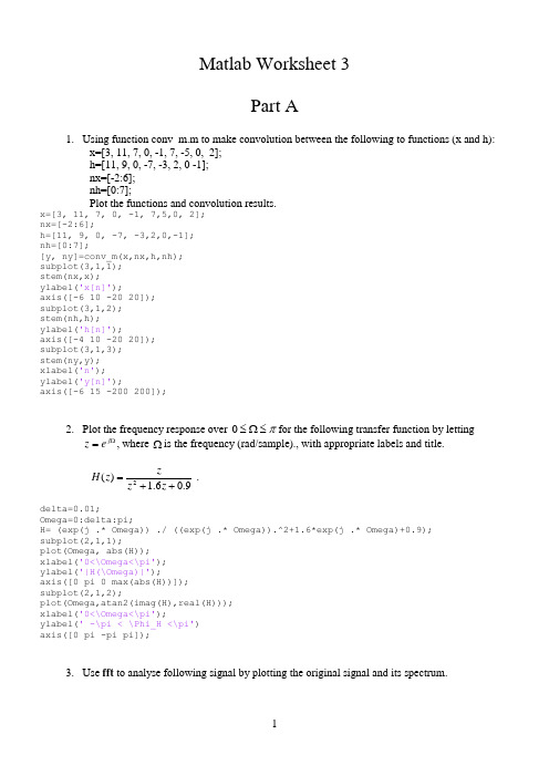
Matlab Worksheet 3Part A1. Using function conv_m.m to make convolution between the following to functions (x and h):x=[3, 11, 7, 0, -1, 7, -5, 0, 2]; h=[11, 9, 0, -7, -3, 2, 0 -1]; nx=[-2:6]; nh=[0:7];Plot the functions and convolution results.x=[3, 11, 7, 0, -1, 7,5,0, 2]; nx=[-2:6];h=[11, 9, 0, -7, -3,2,0,-1]; nh=[0:7];[y, ny]=conv_m(x,nx,h,nh); subplot(3,1,1); stem(nx,x); ylabel('x[n]');axis([-6 10 -20 20]); subplot(3,1,2); stem(nh,h); ylabel('h[n]');axis([-4 10 -20 20]); subplot(3,1,3); stem(ny,y); xlabel('n'); ylabel('y[n]');axis([-6 15 -200 200]);2. Plot the frequency response over π≤Ω≤0for the following transfer function by lettingΩ=j e z , where Ωis the frequency (rad/sample)., with appropriate labels and title.9.06.1)(2++=z z zz H .delta=0.01;Omega=0:delta:pi;H= (exp(j .* Omega)) ./ ((exp(j .* Omega)).^2+1.6*exp(j .* Omega)+0.9); subplot(2,1,1);plot(Omega, abs(H)); xlabel('0<\Omega<\pi'); ylabel('|H(\Omega)|');axis([0 pi 0 max(abs(H))]); subplot(2,1,2);plot(Omega,atan2(imag(H),real(H))); xlabel('0<\Omega<\pi');ylabel(' -\pi < \Phi_H <\pi') axis([0 pi -pi pi]);3. Use fft to analyse following signal by plotting the original signal and its spectrum.⎪⎭⎫ ⎝⎛+⎪⎭⎫ ⎝⎛+⎪⎭⎫ ⎝⎛=10244672sin 10241372sin 1024322sin ][n n n n x πππ.% fft N=1024; dt=1/N;t=0:dt:1-dt;x=sin(2*pi*32 .*t) +sin(2*pi*137 .*t)+sin(2*pi*467 .*t) ; subplot(2,1,1);plot(t,x), xlabel('t sec'),ylabel('x'); title('Signal and its Fourier Transform'); axis([min(t) max(t) 1.5*min(x) 1.5*max(x)]); X=fft(x); f=0:N-1;subplot(2,1,2);stem(f,abs(X)), xlabel('Hz'), ylabel('|X|'); axis([ 0 N/2 0 1.5*max(abs(X))]);4. Use the fast Fourier transform function fft to analyse following signal. Plot the original signal,and the magnitude of its spectrum linearly and logarithmically. Apply Hamming window to reduce the leakage.⎪⎭⎫ ⎝⎛+⎪⎭⎫ ⎝⎛+⎪⎭⎫ ⎝⎛=10247.4672sin 10244.1372sin 10245.322sin ][n n n n x πππ.The hamming window can be coded in Matlab asfor n=1:Nhamming(n)=0.54+0.46*cos((2*n-N+1)*pi/N); end;where N is the data length in the FFT.%Examine signal components %sampling rate 1024Hz N=1024; dt=1/N;t=0:dt:1-dt;%****define the signal**x=0.1*sin(2*pi*32.5 .*t ) + ... 0.2*sin(2*pi*137.4 .*t )+ ... 0.15*sin(2*pi* 467.7 .*t ) ; %*********************** subplot(3,1,1); plot(t,x);axis([0 1 -1 1]);xlabel('nT (seconds)'); ylabel('x[n]');%hamming window for n=1:Nw(n)=0.54+0.46*cos((2*n-N+1)*pi/N); end ;x1=x .*w;subplot(3,1,2); plot(t,x1);axis([0 1 -5 5]);xlabel('nT (seconds)'); ylabel('x[n] Hamming win'); X=fft(x1);df=1;f=0:df:N-1;subplot(3,1,3);plot(f,20*log10(abs(X))); axis([0 N/2 -60 60]);xlabel('k (Hz)');ylabel('|X[k]| (db)');Part BSimulation Using SIMULINKINTRODUCTIONThe objective of this laboratory is to learn about various properties of signals and systems by doing simulations in SIMULINK.PART 1. BASICS OF SIMULINK1.1 UNDERSTANDING SIMPLE WAVEFORMS AND INTEGRATIONCreate a pulse of height 2 units from time 0 to 4 seconds by subtracting two unit steps and adding a gain. Connect this pulse to an integrator with a gain of 0.5 and a zero initial condition. Connect oscilloscopes to show the pulse and the output of the integrator. You may wish to name your simulation (block) diagram; to do so use the save as feature under edit. Your block diagram should be similar as below.Before simulating you need to pull down the simulation header and double click on parameters. Unless told otherwise always assume that you can use the ode 45 integration algorithm shown in this window and the other default parameters. Typically you will only alter the start and stop times but for this first simulation you can use the default values of 0 and 10 seconds. Double click on the oscilloscopes to get the windows in which the traces will appear, pull down the simulate menu and click on run. Plot below the integrator input and output waveforms.Repeat the experiment but with an initial condition of –2 on the integrator. Again draw the results.Repeat the experiment but with an initial condition of –2 on the integrator. Again draw the results.1.2 FIRST ORDER SYSTEMA single time constant may be simulated using the transfer function block in which you enter the coefficients of the numerator and denominator polynomials. Set up the configuration in a new SIMULINK window to realise the transfer function 1/(s+2) with the input unit step and an oscilloscope connected to the output of the transfer function block. Plot the block diagram in the space below. Simulate the system for 5 seconds and plot the response.1.3 SECOND ORDER SYSTEMFor the second order all pole transfer function )2/(200220ωωζω++s s you will recall that if a time scale of ω0t is used for plotting the step response, the response shape will only be affected by changes in the damping ratio ζ. This can also be shown if we normalise the transfer function by replacing (s/ω0) by s n togive )12/(12++n n s s ζ. To study the effect of varying ζ on the step response we will therefore use the transfer function 1/(s 2+2ζs+1). Set up the following configuration for a simulation study.i) A unit step input. ii) Connect the unit step to a transfer function of 1/(s 2+2ζs+1) with ζ = 1.0. iii) Take a summing block and connect the input step to a +ve input and the transfer functionoutput to a –ve input.iv) Connect the output of this summer to a square function. This is obtained by using f(u) in thenonlinear blocks.v)Connect the output of this squarer to an integrator.vi)Connect two oscilloscopes to the circuit, one to the transfer function output and the other to the output of the integrator.vii)Also connect simout blocks to the same signals as the oscilloscopes. Rename the one connected to the integrator output simout1.Simulate the system with the values of ζ listed in the table below and fill in the other figures from the simulation results. To get an accurate value at the end of each run you can type simout1 in the MATLAB window. You can also measure the overshoot by making use of the maximum command: simply type max(simout) in the MATLAB window.% overshoot 2.1076 1.2500 1.1778 1.0571 1.0000 1.1285 2.1431PART 2. SIMULATION OF AIRCRAFT PITCH ANGLE AND ALTITUTEThe purpose IS to use "SIMULINK" to simulate a (much simplified) model of the longitudinal motion of a fighter aircraft.The "angle of attack", is the angle between the direction a plane is pointing, and the direction in which it actually moves through the air. For a plane flying at approximately constant altitude, this is equivalent to the "pitch angle", φ, as illustrated in Fig.2.1. This angle is important because it produces a lift force perpendicular to the axis of the plane, and hence a "normal acceleration", a n , (also shown in the figure).vThe pilot wants to be able to control the pitch angle (倾斜角度), and does so ultimately by rotating the front fins, and tail elevators of the aircraft, shown in Fig. 2.2. The first task is therefore to model theeffect of these movements on the "pitch rate" q ()=φ, and "normal acceleration" a n .Fig. 2.2 Illustration of control surfaces2.1: MODELLING THE AIRCRAFT AND ACTUATOR DYNAMICSi) Normal Acceleration, a nThe acceleration of the aircraft in a direction perpendicular to its axis, (the "normal accel.", a n ), is determined mainly by the angle θ1 of the tail elevators of the aircraft shown in Fig. 2.2. Indeed aerodynamic modelling shows that this relationship can be described by the differential equation,11116342.364.1982.81.3θθθ++=-+ n n n a a aConvert this relationship into a transfer function form:-ii) Pitch Rate, qThe rate at which the pitch angle changes, (the "pitch rate", q ), is determined mainly by the angle θ2 of the front fins of the aircraft shown in Fig. 2.2. Indeed aerodynamic modelling shows that this relationship can be described by the differential equation,2227.1125.782.81.3θθ++=-+ q q qConvert this relationship into a transfer function form:-iii) Actuator Dynamics + GearsThe tail elevators of the aircraft are driven directly by a hydraulic actuator which has a transfer function,G s s ()()=-+1414/ (3)To a unit step input U(s)=1/s , the response R(s) = G(s)⋅U(s)= 1411)14(14++-=+-s s s s . What form ofstep response r(t) would you expect from this actuator, and what is its time constant?The front fins and the tail elevators are both driven from the actuator by the same drive shaft through a gear box. The same gear on this drive shaft connects to the tail elevator gear wheel, which has 500 teeth, and the front fin gear wheel, which has 100 teeth, the relationship between θ1 and θ2 is52112==t t θθ(4) 2.2: SIMULATING THE AIRCRAFT AND ACTUATOR DYNAMICSi) F or the aircraft model you will need from the Continuous or Maths Library:-∙a Transfer Fcn block to represent the "tail elevator angle → normal accel" relationship (eqn (1))∙ a Transfer Fcn block to represent "front fin angle → pitch rate" relationship, (see eqn (2)) ∙ a Transfer Fcn block to represent the hydraulic "actuator dynamics", (see eqn (3)) ∙ a Gain block to represent the "gears", (see eqn (4))from the Sources Library:-∙ a Step Input block to act as a test input - (set Step time = 5sec, and Final value = 0.01 rad)from the Sinks Library:- ∙a ‘Scope block to monitor the pitch rate output - (set Horizontal Range = 20sec).ii) Now connect the blocks together, using the step input to drive the actuator, and the actuator to drive the tail elevators. The actuator is also used to drive the front fins via the gearbox. The 'Scope should be connected to the output of the "front fin angle → pitch rate" block. Note: you can take a branch from a signal line by dragging with the right mouse button from the point on the line at which you want the branch to start.Plot the block diagram you have created in the box below:-iii) From the pull-down menus of your simulation window, select Simulation/Parameters , in order to define how the simulation is to be performed. Set:-Stop Time = 20 sec; Initial Step Size = 0.001; Max Step Size = 0.01;iv) Finally double click on your ‘scope, so that you can watch the progress of the simulation, and then select Simulation/Start from the pull-down menu of your simulation window. You may want to adjustthe Vertical Range of your 'Scope, and re-run the simulation to get a good picture. Plot the response of the aircraft pitch rate below, and comment on these results. Note that it can be shown that if a transfer function has a denominator polynomial with a zero or negative coefficient then it must have a root with a zero or positive real part.2.3: SIMULATING THE PITCH RATE CONTROL SYSTEMThe designers are quite glad they simulated the response of the aircraft, before trying it for real. They now decide to improve the response by measuring the output (ie. what is actually happening to the pitch rate), and subtracting this from the input (ie. what they would like to happen), to produce an error signal. The error signal will be amplified, and then used to drive the actuator (see Fig. 2.3). In this way the actuator will automatically act so as to reduce any differences between the input demand, and the output response.Fig. 2.3 Feedback control of pitch ratei) Before you simulate the control system described above, you will probably find that you are short of space in your simulation window. Besides it would be nice to package the aircraft + actuator dynamics as a single block, so that they are distinct from anything added later as shown in Fig. 2.3.If you press the left mouse button in an empty space of the window, you get a "rubber band" box which you can drag to surround a group of elements. When you release the button, all elements inside are "selected". Use this technique to select all the aircraft + actuator dynamics, (but leave out the step input and ‘scope monitor). From the pull-down menu under Edit select Create a Subsystem, and your diagram will suddenly look as shown in Fig. 2.4.Fig. 2.4 New diagramii) Rename the "Subsystem" as "Actuator + Aircraft Dynamics" as shown in Fig. 2.3 by editing the text below the block. You can see what is inside by double clicking on the block itself, - try it! Notice that the input and output connections are labelled "in_1", "out_1" etc. Edit these to give them more meaningful names.iii) Now construct the planned control system, as illustrated in Fig. 2.3. Notice the pilot is now represented by a Signal Generator (from the Sources library), which should be set to produce a Square Wave, of frequency 0.1 Hz and peak amplitude 0.5.iv) The designers are unsure what value to use for the Gain. Open the Pitch Rate 'Scope, and run the simulation first for the Gain = -0.5 (as shown above), and then for the Gain = -5. Plot the two responses you obtain, and comment on the relative advantages and disadvantages of each:-Comments on responses (in terms of overshot and response time etc):PART 3: SIMILATION OF NONLINEAR SHIP ROLL DYNAMICSThe rolling motion of ships is of considerable interest to naval architects because even today around 50% of ships lost at sea, sink as a result of a capsize. The aim of this laboratory is to study such behaviour by:-∙constructing a nonlinear differential equation model for the system∙converting this model into a phase variable block diagram form suitable for simulation∙simulating the (nonlinear) response to sinusoidal excitation∙calculating the steady state response for a ship whose cargo has shifted dangerously to one sideFig. 3.1 Ship schematic3.1: MODELLING AND SIMULATION OF SHIP DYNAMICSi) Consider the ship sketch shown in Fig. 3.1. Given that:-∙ The effective inertia of the ship about its roll axis = J (1) ∙ The damping moment / torque due to friction between the body of the ship and the water, and due to turbulence round the "bilge keels" = c c 123 θθ+ (2) ∙ The restoring moment / torque due to the buoyancy and shape of the ship, as it is pushed to oneside = k k k 12335θθθ++ (3) ∙ The input / forcing moment due to the wave forces acting on the ship = u t ()- Using Newton’s second law of motion ∑=Torque Moment J / θ , the nonlinear differential equation which describes the rolling motion of the ship can be written as:-()()53321321)(θθθθθθk k k c c t u J ++-+-= (4)(ii) Re-arrange equation (4) to obtain an expression for the highest derivative of the output signal θ:-()()()53321321)(1θθθθθθk k k c c t u J++-+-= (5)iii) Hence complete the drawing of the SIMULINK block diagram for the ship roll system:-3.2: SIMULATING THE SHIP DYNAMICSi) For the ship model you will need:-from the Continuous and Maths Library:-∙ a few Integrator blocks - (assume zero initial conditions for now)∙ a few Gain blocks (not absolutely necessary)from the Nonlinear Library:-∙ a couple of Fcn blocks to implement the damping and stiffness terms (eqns (2), and (3)) from the Sources Library:- ∙ a Sine Wave block to simulate the sea waves u(t) - (set Ampl = 0.3 , and Freq = 0.6 rad/s)from the Sinks Library:-∙ a To Workspace block for the output ship roll angle, θ, of the simulation. This stores the results in a MATLAB variable which we can plot later, -(set the Variable name = theta, and the Maximum number of timesteps (ie points stored) = 5000)∙ an oscilloscope if you wish to see a waveform whilst the simulation is taking placeii) Drag the appropriate blocks over into your simulation window using the mouse, and double click on them to enter the appropriate parameter values. The numerical values for the coefficients of eqn (4) are:-;150;20;8.0;8.0;02.0;132121======k k k c c J(6)Note these values are given in consistent units so that θ is in radians. Finally by clicking on the text under each block, you can also enter a suitable description for each.iii) Now connect the blocks together, according to the phase variable block diagram you have plotted in section A. Note that some blocks will need changing so they "face the other way"; you can do this by selecting the block and "Flipping Horizontally " using the Options pulldown menu. Remember too that you can take a branch from a signal line by dragging with the right mouse button from the point on the line at which you want the branch to start.iv) From the pull-down menus of your simulation window, select Simulation/Parameters , in order to define how the simulation is to be performed. Set:-Stop Time = 10*pi (sec); Initial Step Size = 0.001; Max Step Size = 0.1;v) Now run the simulation by selecting Simulation/Start from the pull-down menu of your simulation window. If you do not use an oscilloscope you probably won't see much happening because the results are being stored in the MATLAB variable called 'theta', instead of being displayed immediately. After a few seconds however, you should hear a slight beep indicating the simulation is complete. Use of an oscilloscope is, however, recommended so that you can see if things ‘look all right’.vi)Now plot your results by typing plot(theta)at the MATLAB prompt in the MATLAB command window. Plot the response below, and comment on how it differs from what you would expect from a linear system if this were also excited with a sine wave input.。
matlab上机作业

第二次 上机作业1、 求下列矩阵的主对角线元素、上三角阵、下三角阵、秩、范数、条件数和迹。
(1)⎥⎥⎥⎥⎦⎤⎢⎢⎢⎢⎣⎡--=901511250324153211A (2)⎥⎦⎤⎢⎣⎡-=2149.824343.0B 1.A=[1,-1,2,3;5,1,-4,2;3,0,5,2;11,15,0,9]D=diag(A)C=triu(A)B=tril(A)E=rank(A)F=trace(A)a1=norm(A,1)a2=norm(A,inf)a3=norm(A,inf)c1=cond(A)c1=cond(A,1)c2=cond(A,2)c3=cond(A,inf)2.B=[0.43,43,2;-8.9,4,21]D=diag(B)C=triu(B)B=tril(B)E=rank(B)F=trace(B)a1=norm(B,1)a2=norm(B,inf)a3=norm(B,inf)c1=cond(B)c1=cond(B,1)c2=cond(B,2)c3=cond(B,inf)2、 求矩阵A 的特征值和相应的特征向量。
⎥⎥⎥⎦⎤⎢⎢⎢⎣⎡=225.05.025.0115.011AA=[1,1,0.5;1,1,0.25;0.5,0.25,2][V ,D]=eig(A)3、 下面是一个线性方程组:⎥⎥⎥⎦⎤⎢⎢⎢⎣⎡=⎥⎥⎥⎦⎤⎢⎢⎢⎣⎡⎥⎥⎥⎦⎤⎢⎢⎢⎣⎡52.067.095.06/15/14/15/14/13/14/13/12/1321x x x (1) 求方程的解。
(2) 将方程右边向量元素3b 改为0.53,再求解,并比较3b 的变化和解的相对变化。
(3) 计算系数矩阵A 的条件数并分析结论。
A=[1/2,1/3,1/4;1/3,1/4,1/5;1/4,1/5,1/6]B=[0.95,0.67,0.52]X=inv(A)*bc1=cond(A,1)c2=cond(A,2)c3=cond(A,inf)4、 利用Matlab 提供的randn 函数生成符合正态分布的10×5随机矩阵A,进行如下操作:(1)A 各列元素的均值和标准方差(2)A 的最大元素和最小元素(3)求A 每行元素的和以及全部元素之和(4)分别对A 的每列元素按升序、每行按降序排列X=randn(10,5)M=mean(X)D=std(X)m=max(X)n=min(X)P=sum(X,2)sum(p)Ans5、按要求对指定函数进行插值(1)按下表用三次样条方法插值计算0~900范围内整数点的正弦值和0~750范围内整数点的正切值。
实验二matlab矩阵分析与处理

《MATLAB及应用A》第二次上机作业一、一球从100米高度自由落下,每次落地后反弹回原高度的一半,再落下。
求它在第10次落下时共经过多少米?第10次反弹多高?MATLAB源程序:MATLAB运行结果:二、有如下一段MATLAB程序,请解释说明每个语句的功能,必要时用数学表达式(不是在MATLAB中的输入形式);并给出y1、y2、y3的值(可从MATLAB中复制)。
MATLAB源程序:x=linspace(0,6);y1=sin(2*x);y2=sin(x.^2);y3=(sin(x)).^2;各条命令语句的功能如下:y1、y2、y3的值分别为:三、教材第55页习题三,第3题。
MATLAB源程序:MATLAB运行结果:四、选择题(1) i=2; a=2i; b=2*i; c=2*sqrt(-1); 程序执行后,a, b, c的值分别是多少?()(A) a=4, b=4, c=2.0000i(B) a=4, b=2.0000i, c=2.0000i(C) a=2.0000i, b=4, c=2.0000i(D) a=2.0000i, b=2.0000i, c=2.0000i(2) 求解方程x4-4x3+12x-9 = 0 的所有解,其结果为()(A) 1.0000, 3.0000, 1.7321, -1.7321(B) 1.0000, 3.0000, 1.7321i, -1.7321i(C) 1.0000i, 3.0000i, 1.7321, -1.7321(D) -3.000-0i, 3.0000i, 1.7321, -1.7321五、求[100,1000]之间的全部素数(选做)。
MATLAB源程序: MATLAB运行结果:一、一球从100米高度自由落下,每次落地后反弹回原高度的一半,再落下。
求它在第10次落下时共经过多少米?第10次反弹多高?MATLAB源程序:>> a=(0:-1:-9) %产生一个行向量aa =0 -1 -2 -3 -4 -5 -6 -7 -8 -9>> b=pow2(a) %对行向量a中的每一个元素分别求幂函数b =1.0000 0.5000 0.2500 0.1250 0.0625 0.0313 0.0156 0.007 8 0.0039 0.0020>> h=100*b %对行向量b中的每一个元素分别乘以100h =100.0000 50.0000 25.0000 12.5000 6.2500 3.1250 1.5625 0. 7813 0.3906 0.1953>> s1=sum(h) %对行向量h中的元素求和s1 =199.8047>> s=s1*2-100 %求出第10次落下时经过的高度s =299.6094>> h10=h(10)/2 %求出第10次反弹的高度h10 =0.0977二、有如下一段MATLAB程序,请解释说明每个语句的功能,必要时用数学表达式(不是在MATLAB中的输入形式);并给出y1、y2、y3的值(可从MATLAB 中复制)。
Matlab上机练习二答案
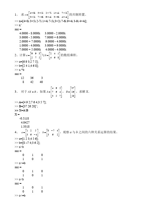
1、 求⎥⎦⎤⎢⎣⎡+-+-+-+-++=i 44i 93i 49i 67i 23i 57i 41i 72i 53i 84x 的共轭转置。
>> x=[4+8i 3+5i 2-7i 1+4i 7-5i;3+2i 7-6i 9+4i 3-9i 4+4i];>> x’ans =4.0000 - 8.0000i 3.0000 - 2.0000i3.0000 - 5.0000i 7.0000 + 6.0000i2.0000 + 7.0000i 9.0000 - 4.0000i1.0000 - 4.0000i 3.0000 + 9.0000i7.0000 + 5.0000i 4.0000 - 4.0000i2、计算⎥⎦⎤⎢⎣⎡=572396a 与⎥⎦⎤⎢⎣⎡=864142b 的数组乘积。
>> a=[6 9 3;2 7 5];>> b=[2 4 1;4 6 8];>> a.*bans =12 36 38 42 403、 对于B AX =,如果⎥⎥⎥⎦⎤⎢⎢⎢⎣⎡=753467294A ,⎥⎥⎥⎦⎤⎢⎢⎢⎣⎡=282637B ,求解X 。
>> A=[4 9 2;7 6 4;3 5 7];>> B=[37 26 28]’;>> X=A\BX =-0.51184.04271.33184、 ⎥⎦⎤⎢⎣⎡-=463521a ,⎥⎦⎤⎢⎣⎡-=263478b ,观察a 与b 之间的六种关系运算的结果。
>> a=[1 2 3;4 5 6];>> b=[8 –7 4;3 6 2];>> a>bans =0 1 01 0 1>> a>=bans =0 1 01 0 1>> a<bans =1 0 10 1 0>> a<=bans =1 0 10 1 0>> a==bans =0 0 00 0 0>> a~=bans =1 1 11 1 15、[]7.0802.05--=a ,在进行逻辑运算时,a 相当于什么样的逻辑量。
matlab实验报告2

第二次上机作业准备&要求:1、 运行课件第三章(课本第四章)讲过的例子,掌握Matlab 的流程控制语句、函数及脚本文件的编程、调试方法。
2、 本次作业(4~12题)要求全部写M 文件;3、 题目要求未明确要求写脚本文件还是函数文件的,学生自己决定是写脚本文件还是函数文件。
只要能够实现要求。
4、 列出第二章课堂上出现过的所有函数,知道它们的作用并试着调用这些函数。
作业:1. 继续完成第一次上机实验未完成的作业。
2. 分析脚本M 文件及函数M 文件的区别。
(1)脚本文件没有输入参数,也不返回输出参数,而函数文件可以带输入参数,也可以返回输出参数。
(2)脚本文件对MATLAB 工作空间中的变量进行操作,文件中所有命令的执行结果也完全返回到工作空间中,而函数文件中定义的变量为局部变量,当函数文件执行完毕时。
这些变量被清除。
(3)脚本文件可以直接运行。
在MATLAB 命令行窗口输入脚本文件的名字,就会顺序执行脚本文件中的命令。
而函数文件不能直接运行,要以函数调用的方式来调用。
3. 已知⎥⎥⎥⎦⎤⎢⎢⎢⎣⎡--=7613870451A ,⎥⎥⎥⎦⎤⎢⎢⎢⎣⎡--=023352138B ,求下列表达式的值,并注意第(2)(3)小题表达式的结果有何特点:(1)B A 6+ 、I B A +-2(其中I 为单位阵);>> A+6*Bans =47 23 -1012 37 26-15 73 7>> A^2-B+Ians =-18 -217 1722 533 10921 867 526(2)A*B、A.*B、B*A、B.*A;>> A*Bans =14 14 16-10 51 21125 328 180>> A.*Bans =-8 15 40 35 24-9 122 0>> B*Aans =-11 0 -157 228 533 -1 28>> B.*Aans =-8 15 40 35 24-9 122 0(3)A/B、B\A、A./B、B.\A;A/Bans =1.2234 -0.92552.9787-0.9468 2.3511 -0.95744.6170 3.8723 13.8936>> B\Aans =-0.5106 -8.6170 -1.12770.7340 17.5745 1.8085-0.8830 -21.2128 0.4043>> A./Bans =-0.1250 1.6667 4.00000 1.4000 2.6667-1.0000 30.5000 Inf>> B.\Aans =-0.1250 1.6667 4.00000 1.4000 2.6667-1.0000 30.5000 Inf(4)[A, B]、[A([1 3],:);B^2]。
Matlab第二、三次上机作业-推荐下载

第二次上机作业一. 任务: 用MATLAB 语言编写连续函数最佳平方逼近的算法程序(函数式M 文件)。
并用此程序进行数值试验,写出计算实习报告。
二. 程序功能要求:1.用Lengendre 多项式做基,并适合于构造任意次数的最佳平方逼近多项式。
可利用递推关系0112()1,()()(21)()(1)()/2,3,.....n n n P x P x x P x n xP x n P x nn --===---⎡⎤⎣⎦=2.程序输入:(1)待求的被逼近函数值的数据点(可以是一个数值或向量)0x (2)区间端点:a,b 。
3. 程序输出:(1)拟合系数:012,,,...,nc c c c (2)待求的被逼近函数值00001102200()()()()()n n s x c P x c P x c P x c P x =++++ 三:数值试验要求:1.试验函数:;也可自选其它的试验函数。
()cos ,[0,4]f x x x x =∈+2.用所编程序直接进行计算,检测程序的正确性,并理解算法。
3.分别求二次、三次、。
最佳平方逼近函数。
)x s (4.分别作出逼近函数和被逼近函数的曲线图进行比较。
)x s ()(x f (分别用绘图函数plot(,s())和fplot(‘x cos x ’,[x 1 x 2,y 1,y 2]))0x 0x 解题思路:参照应用数值分析书P259“算法7-1”,利用Legendre 多项式对f(x)∈C(a,b)的最佳平方逼近写出以下算法:M 文件1:%文件名:GLAppro.mfunction[poly,yy,delta]=GLAppro(f,n,a,b,xx)%功能:利用Gauss Legendre 多项式求函数的最佳平方逼近%输入:f ——被逼近函数;a,b ——逼近区间;xx ——欲求的逼近点%n ——逼近的L 多项式的次数(标量时为最高次数,向量时为其所选择的的逼近次数)%输出:poly ——所求的逼近多项式系数(降序);yy ——逼近店的值;delta ——逼近误差N=numel(n);if N>1id=n+1;elseN=n+1;enddelta=quad(@myfun,-1,1,[],[],f,a,b);c=zeros(1,N);poly=zeros(1,id(N)); for k=1:Nc(k)=(2*id(k)-1)*quad(@fLegPoly,-1,1,[],[],f,id(k)-1,a,b)/2;delta=delta-c(k)^2*2/(2*id(k)-1);endif nargin==5t0=(2*xx-a-b)/(b-a);yy=zeros(size(xx));for k=1:Np=LegPoly(id(k)-1);yy=yy+c(k)*polyval(p,t0);poly(id(N)-id(k)+1:(id(N)))=poly(id(N)-id(k)+1:(id(N)))+c(k)*p;endelsefor k=1:Np=LegPoly(k-1);poly(N-k+1:N)=poly(N-k+1:N)+c(k)*p;endendM文件2:function y=myfun(t,f,a,b)%功能:GLAppro子函数,变换到区间[-1,1]x=(b-a)*t/2+(b+a)/2;y=f(x).*f(x);M文件3:function f=fLegPoly(t,f1,n,a,b)%功能:GLAppro子函数,求变换后的积分函数p=LegPoly(n);x=(b-a)*t/2+(b+a)/2;f=f1(x).*polyval(p,t);M文件4:function p=LegPoly(n)%功能:递归法求n次Gauss Legendre多项式%输入:n——多项式次数%输出:p——降幂排列的多项式系数p0=1;p1=[1,0];if n==0p=p0;elseif n==1p=p1;elsep=((2*n-1)*[LegPoly(n-1),0]-(n-1)*[0,0,LegPoly(n-2)])/n;end%文件名:homework2.mf=@(x)(x.*cos(x));n=cell(3,1);n{1}=2;n{2}=3;n{3}=4;a=0;b=4;x0=linspace(a,b)';color=['k','g','b'];y=f(x0);plot(x0,y,'r-','linewidth',1.5);hold on;syms t x;for i=1:3[poly,py,delta]=GLAppro(f,n{i},a,b,x0);pt=vpa(poly2sym(poly,t),4);poly=simple(subs(pt,t,(2*x-a-b)/(b-a)));poly=vpa(poly,4);disp(['所求的最佳评分那个逼近多项式为(n=' int2str(n{i}) '):']);disp(poly);disp(['误差为:' num2str(delta)]);plot(x0,py,color(i),'linewidth',1.5)end分别求两次、三次和四次最佳平方逼近函数s(x)输入:homework2输出:所求的最佳评分那个逼近多项式为(n=2):- 0.1599*x^2 - 0.572*x + 0.8268误差为:0.45032所求的最佳评分那个逼近多项式为(n=3):0.3818*x^3 - 2.45*x^2 + 3.093*x - 0.3948误差为:0.02393所求的最佳评分那个逼近多项式为(n=4):0.08539*x^4 - 0.3014*x^3 - 0.6939*x^2 + 1.531*x - 0.08255误差为:0.002258调整图象并标注:yx第三次上机作业一. 任务一:用MATLAB 语言编写化工原理流体力学中d-u-Re-λ试差法的算法程序(函数式M 文件)。
Matlab上机作业部分参考答案

3. 设A为 数组,B为一个行数大于3的数组,请给出 (1)删除A的第4、8、12三列的命令; (2)删除B的倒数第3行的命令; (3)求符号极限 (4)求 的3阶导数
lim tan( mx ) 的命令集; x 0 nx x3 y arctan ln(1 e 2 x ) 的命令集; x2
1 0.8 0.6 0.4 0.2 0 -0.2 -0.4 -0.6 -0.8
0
2
4
6
8
10
12
14
某校60名学生的一次考试成绩如下: 93 75 83 93 91 85 84 82 77 76 77 95 94 89 91 88 86 83 96 81 79 97 78 75 67 69 68 84 83 81 75 66 85 70 94 84 83 82 80 78 74 73 76 70 86 76 90 89 71 66 86 73 80 94 79 78 77 63 53 55 1)计算均值、标准差、极差、偏度、峰度,画出直方图; 2)检验分布的正态性; 3)若检验符合正态分布,估计正态分布的参数并检验参数。 解答: x=[93 75 83 93 91 85 84 82 77 76 77 95 94 89 91 88 86 83 96 81 79 97 78 75 67 69 68 84 83 81 75 66 85 70 94 84 83 82 80 78 74 73 76 70 86 76 90 89 71 66 86 73 80 94 79 78 77 63 53 55]; mean(x) std(x) range(x) skewness(x) kurtosis(x) hist(x) h=normplot(x) [muhat,sigmahat,muci,sigmaci]=normfit(x) [H,sig,ci]=ttest(x,80.1)
《MATLAB及应用》上机作业-2015.doc
《MA TLAB及应用》上机作业学院名称:(四号宋体)专业班级:(四号宋体)学生姓名:(四号宋体)学生学号:(四号宋体)年月《MATLAB及应用》上机作业要求及规范一、作业提交方式:word文档打印后提交。
二、作业要求:1.封面:按要求填写学院、班级、姓名、学号,不要改变封面原有字体及大小。
2.内容:只需解答过程(结果为图形输出的可加上图形输出结果),不需原题目;为便于批阅,题与题之间应空出一行;每题答案只需直接将调试正确后的M文件内容复制到word 中(不要更改字体及大小),如下所示:%作业1_1clcA=[1 2 3 4;2 3 5 7;1 3 5 7;3 2 3 9;1 8 9 4];B=[1+4*i 4 3 6 7 7;2 3 3 5 5 4+2*i;2 6+7*i 5 3 4 2;1 8 9 5 4 3];C=A*BD=C(4:5,4:6)三、大作业评分标准:1.提交的打印文档是否符合要求;2.作业题的解答过程是否完整和正确;3.答辩过程中阐述是否清楚,问题是否回答正确;4.作业应独立完成,严禁直接拷贝别人的电子文档,发现雷同者都以无成绩论处。
作业11、用MATLAB 可以识别的格式输入下面两个矩阵12342357135732391894A ⎛⎫⎪⎪ ⎪= ⎪⎪ ⎪⎝⎭,144367723355422675342189543i i B i +⎛⎫⎪+⎪= ⎪+ ⎪⎪⎝⎭再求出它们的乘积矩阵C ,并将C 矩阵的右下角23⨯子矩阵赋给D 矩阵。
赋值完成后,调用相应的命令查看MATLAB 工作空间的占有情况。
2、设矩阵16231351110897612414152⎛⎫⎪⎪ ⎪ ⎪⎝⎭,求A ,1A -,3A ,12A A -+,1'3A A --,并求矩阵A 的特征值和特征向量。
3、解下列矩阵方程:010100143100001201001010120X -⎛⎫⎛⎫⎛⎫⎪ ⎪ ⎪=- ⎪ ⎪ ⎪ ⎪ ⎪ ⎪-⎝⎭⎝⎭⎝⎭ 4、求多项式322()(53513)(453)(313)f x x x x x x x =++++++当3x =时的值,并求()f x 的导数。
MATLAB第3次上机作业
hls=det(a) %(1)计算行列式; njz=inv(a) %(1)计算逆矩阵; [tzxl,tzz]=eig(a) %(2)计算特征向量和特征值; Jtx=rref(a) %(3)化为行最简单的阶梯形; zzs=[]; fori=1:4
zzs=[zzs,det(a(1:i,1:i))]; end zzs %(5)求顺序主子式 %(5)求特征值之和; %(5)求主对角元之和;
%求特解 %求 AX=0 的基础-0.533333333333333 0.600000000000000
C=
1.500000000000000
-0.750000000000000 1.750000000000000 0 1.000000000000000
1.500000000000000 1.000000000000000 0
-0.481933427298575 -0.629136472171865 -0.276571160291259 0.599472951677392 0.317787492557903
-0.502916831096254 -0.463014344487770 tzz = 2.402116769571056 0 0 -0.034553097766873 0 0 0 0 0 0.057018866656021
y=(1+cos(u)).*sin(v); z=sin(u); mesh(x,y,z)
运行结果: 6. 产生一个 4 阶的随机矩阵,执行下面的操作: 求其行列式,检验其是否可逆;若可逆,求其逆矩阵。 计算该矩阵的特征值、特征向量。 将该矩阵化为行最简的阶梯形。 验证矩阵的特征值之和等于矩阵主对角元之和,特征值之积等于矩阵的行列 式。 a=rand(4) %产生一个 4 届随机矩阵;
Matlab上机作业部分参考答案

上机练习二 参考答案
1. 产生一个1x10的随机矩阵,大小位于(-5 5),并 且按照从大到小的顺序排列好! 【求解】 a=10*rand(1,10)-5; b=sort(a,'descend')
上机练习二 参考答案
2、用MATLAB 语句输入矩阵A 和B
前面给出的是4 ×4 矩阵,如果给出A(5,6) = 5 命令,矩阵A将得出什么 结果?
Matlab 上机课作业
吴梅红 2012.10.15
上机练习一
上机练习一 参考答案
上机练习一 参考答案
上机练习一 参考答案
上机练习二
1. 产生一个1x10的随机矩阵,大小位于(-5 5),并且按 照从大到小的顺序排列好! 2、用MATLAB 语句输入矩阵A 和B
前面给出的是4 ×4 矩阵,如果给出A(5,6) = 5 命令,矩阵 A将得出什么结果? 3、假设已知矩阵A ,试给出相应的MATLAB 命令,将其全 部偶数行提取出来,赋给B 矩阵,用A =magic(8) 命令生成A 矩阵,用上述的命令检验一下结果是不是正确。
【求解】用课程介绍的方法可以直接输入这两个矩阵 >> A=[1 2 3 4; 4 3 2 1; 2 3 4 1; 3 2 4 1] A= 1234 4321 2341 3241 若给出A(5,6)=5 命令,虽然这时的行和列数均大于A矩阵当前的维数, 但仍然可以执行该语句,得出 >> A(5,6)=5 A= 123400 432100 234100 324100 000005 复数矩阵也可以用直观的语句输入 3+2i 4+1i; 4+1i 3+2i 2+3i 1+4i; 2+3i 3+2i 4+1i 1+4i; 3+2i 2+3i 4+1i 1+4i]; B= 1.0000 + 4.0000i 2.0000 + 3.0000i 3.0000 + 2.0000i 4.0000 + 1.0000i 4.0000 + 1.0000i 3.0000 + 2.0000i 2.0000 + 3.0000i 1.0000 + 4.0000i 2.0000 + 3.0000i 3.0000 + 2.0000i 4.0000 + 1.0000i 1.0000 + 4.0000i 3.0000 + 2.0000i 2.0000 + 3.0000i 4.0000 + 1.0000i 1.0000 + 4.0000i
MATLAB第三次上机实验
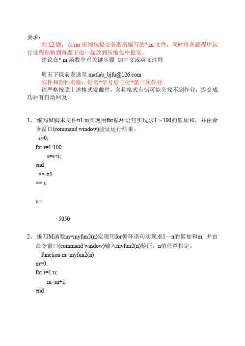
第三次上机实验一.实验目的:进一步了解MATLAB软件的使用,完成曲线图的绘制及各类积分等题型的求解。
二.实验内容及步骤:(1)在同一坐标系下绘制t2,-t2,t2sin t在[0,2]∈内的曲线图;选择tπ合适的“曲线线型”,“曲线颜色”、“标记符号”选项,并在图形上加注坐标轴名和图名。
t=0:pi/100:2*pi;y=t.^2;y1=-t.^2;y2=t.^2.*sin(t);plot(t,y,’—r’,t,y1,;-.g’,t,y2,’x’)t(2)选择合适的θ的范围,讲同一图形窗口分割成2行2列绘制下列4幅极坐标图23(1) 1.0013(2)cos(3.5)sin (3)(4)1cos (7)ρθρρρθθθθ====-t=0:0.1:8*pi; y1=1.0013.*t.^2; y2=cos(3.5*t); y3=sin(t)./t; y4=1-(cos(7.*t)).^3; subplot(2,2,1),polar(t,y1); subplot(2,2,2),polar(t,y2); subplot(2,2,3),polar(t,y3); subplot(2,2,4),polar(t,y4);(3)用鼠标左键在图形窗口上取5个点,在每个点的位置处写出一个字符串来显式鼠标点的横坐标值,然后将这些点连成折线。
axis([0,5,0,5]);hold on;box on;x=[];y=[];gtext('');for i=1:5[x1,y1,button]=ginput(1);if(button~=1)break;endplot(x1,y1,'o');x=[x,x1];y=[y,y1];text(x1,y1,num2str(x1));line(x,y); end hold off(4)求积分40()a f x dx=⎰,其中2ln ,()ln16,22sin(1)2x if x f x if x x π⎧⎪=⎨>⎪++⎩≤f1=inline('log(x.^2)','x');f2=inline('log(16)./(2+sin((x+1).*pi))','x'); [s1,kk]=quad(f1,0,2); [s2,kk]=quad(f2,2,4); s=s1+s2 s =0.511.522.533.544.5500.511.522.533.544.551.9741(5)求解方程x5+6x4-3x2=10的5个根,并将其位置用五角星符号标记在复平面上,要求横纵坐标轴刻度等长,注明虚轴和实轴,在title位置上写出方程。
matlab第三次作业
i 3 10000 的最小 m 值,由命令窗 i 1
m
口(command window)验证运行结果。
值, , 函数输入值为 n, 返回值为 m 和 s, 由命令窗口(command window)输入[m, sum]=myfun7(20000)验证。
function [m,sum]=myfun7(n) m=0; sum=0;
>> ans = 30.6998 >> 9.使用 switch+case 语句编写如下函数 jijie=myfun9(yue),当时输入 12,1,2 时输出 winter, 当时输入 3, 4, 5 时输出 spring, 当时输出 autumn。 结果由命令窗口(command window)输入 myfun9(7)和 s=myfun9(11)验证。 function jijie=myfun9(yue) switch(yue) case {3 4 5} jijie='spring'; case {6 7 8} jijie='summer'; case {9 10 11} jijie='autumn'; case {12 1 2} jijie='winter'; end > myfun9(7) ans = summer >> myfun9(11) ans =
贴到 word 中)
12.编写一个 M 脚本文件 ti12.,m,使用 plot 命令绘制 y=sinx+cosx 的结果图, 其中 x=0:0.1:2π ,计算结果,要求曲线为红色线,菱形符数据点形,图名: “cosx+sinx” ; x 坐标轴名: “x 值” ;y 坐标名: “cosx+sinx 值” ;显示分格线。 绘图结果粘贴到下面:
MATLAB上机作业

MATLAB上机作业MATLAB 上机作业1对以下问题,编写M 文件:(1) 用起泡法对10个数由小到大排序。
即将相邻两个数比较,将小的调到前头。
function f=qipaofa(x) for j=9:-1:1 for i=1:j if(x(i)>x(i+1))t=x(i);x(i)=x(i+1);x(i+1)=t; end end end f=xx=round(10*rand(1,10)) qipaofa(x);(2) 有一个4×5矩阵,编程求出其最大值及其所处的位置。
function f=zuidazhi(x) a=1;b=1;c=x(1,1); for i=1:4 for j=1:5 if x(i,j)>ca=i;b=j;c=x(i,j); end end endf=[c,a,b]x=rand(4,5) zuidazhi(x)(3) 编程求∑=201!n n 。
function f=qiuhe(x) b=0; for i=1:x a=prod(1:i); b=b+a; end f=bqiuhe(20)(4)一球从100米高度自由落下,每次落地后反跳回原高度的一半,再落下。
求它在第10次落地时,共经过多少米?第10次反弹有多高? function f=gao(x)b=x; for i=2:10 x=x/2; a=x*2; b=b+a; end f=[b x/2]gao(100)(5)有一函数y xy xy x f 2sin ),(2++=,写一程序,输入自变量的值,输出函数值。
Function f=fun(x)f=x(1)^2+sin(x(1)*x(2))+2*x(2)MATLAB 上机作业21. 求和4024441++++= Y 。
syms k s=4^k;S=symsum(s,k,0,40)2. 求函数71862)(23+--=x xx x f 的极值,并作图。
第一、二次上机练习

第一、二次上机练习:目的:1.Matlab 的安装、卸载:(选作,自己有电脑的可以做) 2.建立自己的工作目录,再将自己的工作目录设置到matlab 的搜索路径下。
3.掌握MATLAB 各种表达式的书写规则 4.运行课堂上讲过的例子,熟悉矩阵、表达式的基本操作和运算。
作业:1. 求下列表达式的值,显示MATLAB 工作空间的使用情况并保存全部变量:(1))1034245.01(26-⨯+⨯=ww=sqrt(2)*(1+0.34245*10^-6)w =1.4142(2),)tan(22ac b e abc c b a x ++-+++=ππ 其中a=3.5,b=5,c=9.8。
>> a=3.5;b=5;c=9.8;>> x=(2*pi*a+(b+c)/(pi+a*b*c)-exp(2))/(tan(b+c)+a)x =6.6186(3)])48333.0()41[(22απβππα---=y ,其中32.3=α,9.7-=β>> m=3.32;n=-7.9;>> y=2*pi*m^2*((1-pi/4)*n-(0.8333-pi/4)*m)y =(4))1ln(2122t t e z t ++=,其中⎥⎦⎤⎢⎣⎡--=65.05312i t >> t=[2,1-3*i;5,-0.65];>> z=exp(2*t)*log(t+sqrt(1+t^2))/2z =1.0e+004 *0.0057 - 0.0007i 0.0049 - 0.0027i1.9884 - 0.3696i 1.7706 - 1.0539i2. 已知⎥⎥⎥⎦⎤⎢⎢⎢⎣⎡--=7613870451A ,⎥⎥⎥⎦⎤⎢⎢⎢⎣⎡--=023352138B ,求下列表达式的值: (1)B A 6+、I B A +-2(其中I 为单位阵);(2)A*B 、A.*B 、B*A 、B.*A ;(3)A/B 、B\A ;(4)[A, B]、[A([1 3],:);B^2]。
- 1、下载文档前请自行甄别文档内容的完整性,平台不提供额外的编辑、内容补充、找答案等附加服务。
- 2、"仅部分预览"的文档,不可在线预览部分如存在完整性等问题,可反馈申请退款(可完整预览的文档不适用该条件!)。
- 3、如文档侵犯您的权益,请联系客服反馈,我们会尽快为您处理(人工客服工作时间:9:00-18:30)。
计算示例 2:
方程式转化为:lgP = A + lgP0 −
������������0 ������
命 lgP = y, T = x 构造函数 y = A + lgP0 − ������������0 ������
1
首先用 exel 进行数据预处理,并可得到线性拟合结果,右图:
T/℃ 0 20 40 60 80 100 120 140 160
M 文件 2: function [d,u,Re,s,i]=ccshicha(hf,l,v,p,cp,e)
cp:液
%函数为试差法计算粗糙管管径及流速 %输入:hf:压头损失/m l:管长/m v:流量/(m3/h) p:液体密度/(kg/m3) cp:液体粘 度/(Pa·s) e:粗糙度/mm %输出:d:管径/m u:流速/(m/s) Re:雷诺数 s:摩擦系数 i:迭代次数 s=0.001; for i=1:1000 ss=s; d=(s*v*v*l/(3600*3600*15.41*hf))^(1/5); u=v/(3600*0.78539815*d*d); Re=d*u*p/cp; s=0.100*(e/1000*d+68/Re)^0.23; if s-ss<0.0001 break end end 三、结果检测: 1、 输入:[d,u,Re,s,i]=ghshicha(4.5,70,30,1000,0.001) 输出:d =0.0648u =2.5299Re =1.6384e+005s =0.0163i =3 2、 输入:[d,u,Re,s,i]=ccshicha(4.5,70,30,1000,0.001,0.2) 输出:d =0.0651u =2.5010Re =1.6290e+005s =0.0168i =3 结果显示, 粗糙管由于存在摩擦消耗, 相应的管径要加粗一些才能使输送压头损失保持 在 4.5m。通过编写该算法,日后遇到相同或相似问题可直接调用程序进行计算,不必再人 工手算,提高时效性。
P/kPa 1.589 5.87 17.89 46.81 108.2 223.6 423.9 747.4 1240
1/T(1/K) 0.003663 0.003413 0.003195 0.003003 0.002833 0.002681 0.002545 0.002421 0.002309
lgP 0.201124 0.768638 1.25261 1.670339 2.034227 2.349472 2.627263 2.873; end delta=quad(@myfun,-1,1,[],[],f,a,b);c=zeros(1,N);poly=zeros(1,id(N)); for k=1:N c(k)=(2*id(k)-1)*quad(@fLegPoly,-1,1,[],[],f,id(k)-1,a,b)/2; delta=delta-c(k)^2*2/(2*id(k)-1); end if nargin==5 t0=(2*xx-a-b)/(b-a);yy=zeros(size(xx)); for k=1:N p=LegPoly(id(k)-1);yy=yy+c(k)*polyval(p,t0); poly(id(N)-id(k)+1:(id(N)))=poly(id(N)-id(k)+1:(id(N)))+c(k)*p; end else for k=1:N p=LegPoly(k-1);poly(N-k+1:N)=poly(N-k+1:N)+c(k)*p; end end
三:数值试验要求: 1. 试验函数: f ( x ) x cos x , x [0, 4] ;也可自选其它的试验函数。 2. 用所编程序直接进行计算,检测程序的正确性,并理解算法。 3. 分别求二次、三次、 。 。 。最佳平方逼近函数 s( x) 。 4. 分别作出逼近函数 s( x) 和被逼近函数
M 文件 2:
function y=myfun(t,f,a,b) %功能:GLAppro 子函数,变换到区间[-1,1] x=(b-a)*t/2+(b+a)/2;y=f(x).*f(x);
M 文件 3:
function f=fLegPoly(t,f1,n,a,b) %功能:GLAppro 子函数,求变换后的积分函数 p=LegPoly(n); x=(b-a)*t/2+(b+a)/2; f=f1(x).*polyval(p,t);
调整图象并标注:
1 真值 逼近次数:2 逼近次数:3 逼近次数:4
0
-1
-2
y
-3
-4
-5
0
0.5
1
1.5
2 x
2.5
3
3.5
4
第三次上机作业
一. 任务一: 用 MATLAB 语言编写化工原理流体力学中 d-u-Re-λ 试差法的算法程序(函数式 M 文 件) 。并用此程序进行数值试验,写出计算实习报告。 任务二: 用 MATLAB 语言编写物理化学气液平衡实验数据拟合的算法程序(函数式 M 文件) 。 并用此程序进行数值试验,写出计算报告。 二. 程序功能: 通过编写迭代的算法程序, 使得常规计算过程的人工手算方法得以程序化, 节省时间且 计算准确。 计算示例 1: 一管路总长 70m,要求输水量 30m3/h,输送过程的允许压头损失为 4.5m 水柱。求管径 d。已知水的密度为 1000kg/m3,粘度为 0.001Pa· s; (1)管为光滑管; (2)管内部的绝对粗糙度为 0.2mm。 解: 在此过程中需要用到以下公式:
M 文件 4:
function p=LegPoly(n) %功能:递归法求 n 次 Gauss Legendre 多项式 %输入:n——多项式次数 %输出:p——降幂排列的多项式系数 p0=1;p1=[1,0]; if n==0 p=p0; elseif n==1 p=p1; else p=((2*n-1)*[LegPoly(n-1),0]-(n-1)*[0,0,LegPoly(n-2)])/n; end
2. 程序输入: 3. 程序输出: (1)待求的被逼近函数值的数据点 x 0 (可以是一个数值或向量) (2)区间端点:a,b。 (1)拟合系数: c0 , c1 , c2 ,..., cn (2)待求的被逼近函数值
s( x0 ) c0 P0 ( x0 ) c1 P1 ( x0 ) c2 P2 ( x0 ) cn Pn ( x0 )
分别求两次、三次和四次最佳平方逼近函数 s(x) 输入: homework2 输出: 所求的最佳评分那个逼近多项式为(n=2): - 0.1599*x^2 - 0.572*x + 0.8268 误差为:0.45032 所求的最佳评分那个逼近多项式为(n=3): 0.3818*x^3 - 2.45*x^2 + 3.093*x - 0.3948 误差为:0.02393 所求的最佳评分那个逼近多项式为(n=4): 0.08539*x^4 - 0.3014*x^3 - 0.6939*x^2 + 1.531*x - 0.08255 误差为:0.002258
第二次上机作业
一. 任务: 用 MATLAB 语言编写连续函数最佳平方逼近的算法程序(函数式 M 文件) 。并用此程序进 行数值试验,写出计算实习报告。 二. 程序功能要求: 1. 用 Lengendre 多项式做基,并适合于构造任意次数的最佳平方逼近多项式。
P0 ( x ) 1, P1 ( x ) x 可利用递推关系 Pn ( x ) (2n 1) xPn 1 ( x ) ( n 1) Pn 2 ( x ) / n n 2, 3, .....
M 文件 5:
%文件名:homework2.m f=@(x)(x.*cos(x));n=cell(3,1);n{1}=2;n{2}=3;n{3}=4; a=0;b=4;x0=linspace(a,b)';color=['k','g','b']; y=f(x0);plot(x0,y,'r-','linewidth',1.5);hold on;syms t x; for i=1:3 [poly,py,delta]=GLAppro(f,n{i},a,b,x0);pt=vpa(poly2sym(poly,t),4); poly=simple(subs(pt,t,(2*x-a-b)/(b-a)));poly=vpa(poly,4); disp(['所求的最佳评分那个逼近多项式为(n=' int2str(n{i}) '):']);disp(poly); disp(['误差为:' num2str(delta)]);plot(x0,py,color(i),'linewidth',1.5) end
f ( x ) 的曲线图进行比较。
(分别用绘图函数 plot( x 0 ,s( x 0 ))和 fplot(‘xcosx’,[x1 x2,y1,y2]))
解题思路:参照应用数值分析书 P259“算法 7-1” ,利用 Legendre 多项式对 f(x)∈C(a,b)的最 佳平方逼近写出以下算法: M 文件 1:
(4)为光滑管摩擦系数计算公式 (5)为粗糙管摩擦系数计算公式 设定λ 初值,带入进行试差,直到计算出的λ 与上一个λ 相差在误差范围内时,试 差结束。 1、算法程序编写 以下为相应算法:
M 文件 1: function [d,u,Re,s,i]=ghshicha(hf,l,v,p,cp) %函数为试差法计算光滑管管径及流速 %输入:hf:压头损失/m l:管长/m v:流量/(m3/h) p:液体密度/(kg/m3) 体粘度/(Pa·s) %输出:d:管径/m u:流速/(m/s) Re:雷诺数 s:摩擦系数 i:迭代次数 s=0.001; for i=1:1000 ss=s; d=(s*v*v*l/(3600*3600*15.41*hf))^(1/5); u=v/(3600*0.78539815*d*d); Re=d*u*p/cp; s=0.0056+0.500/Re^0.32; if s-ss<0.0001 break end end