第11 章 深度图(Depth Map)
深度图像的获取原理

深度图像的获取原理RGB-D(深度图像) 深度图像 = 普通的RGB三通道彩⾊图像 + Depth Map 在3D计算机图形中,Depth Map(深度图)是包含与视点的场景对象的表⾯的距离有关的信息的图像或图像通道。
其中,Depth Map类似于灰度图像,只是它的每个像素值是传感器距离物体的实际距离。
通常RGB图像和Depth图像是配准的,因⽽像素点之间具有⼀对⼀的对应关系。
下⾯可以看到两个不同的深度图,以及从中衍⽣的原始模型。
第⼀个深度图显⽰与照相机的距离成⽐例的亮度。
较近的表⾯较暗; 其他表⾯较轻。
第⼆深度图⽰出了与标称焦平⾯的距离相关的亮度。
靠近焦平⾯的表⾯较暗; 远离焦平⾯的表⾯更轻((更接近并且远离视点)。
⽴⽅体结构深度图:更近更深深度图:近距离焦距更深 RGB-D Dataset: RGB-D Demo:图像深度 图像深度是指存储每个像素所⽤的位数,也⽤于量度图像的⾊彩分辨率。
图像深度确定彩⾊图像的每个像素可能有的颜⾊数,或者确定灰度图像的每个像素可能有的灰度级数。
它决定了彩⾊图像中可出现的最多颜⾊数,或灰度图像中的最⼤灰度等级。
⽐如⼀幅单⾊图像,若每个像素有8位,则最⼤灰度数⽬为2的8次⽅,即256。
⼀幅彩⾊图像RGB 三通道的像素位数分别为4,4,2,则最⼤颜⾊数⽬为2的4+4+2次⽅,即1024,就是说像素的深度为10位,每个像素可以是1024种颜⾊中的⼀种。
例如: ⼀幅画的尺⼨是1024*768,深度为16,则它的数据量为1.5M。
计算如下: 1024×768×16 bit = (1024×768×16)/8 Byte = [(1024×768×16)/8]/1024 KB = 1536 KB = {[(1024×768×16)/8]/1024}/1024 MB = 1.5 MB。
(整理)第11章深度图
第十一章 深度图获取场景中各点相对于摄象机的距离是计算机视觉系统的重要任务之一.场景中各点相对于摄象机的距离可以用深度图(Depth Map)来表示,即深度图中的每一个像素值表示场景中某一点与摄像机之间的距离.机器视觉系统获取场景深度图技术可分为被动测距传感和主动深度传感两大类.被动测距传感是指视觉系统接收来自场景发射或反射的光能量,形成有关场景光能量分布函数,即灰度图像,然后在这些图像的基础上恢复场景的深度信息.最一般的方法是使用两个相隔一定距离的摄像机同时获取场景图像来生成深度图.与此方法相类似的另一种方法是一个摄象机在不同空间位置上获取两幅或两幅以上图像,通过多幅图像的灰度信息和成象几何来生成深度图.深度信息还可以使用灰度图像的明暗特征、纹理特征、运动特征间接地估算.主动测距传感是指视觉系统首先向场景发射能量,然后接收场景对所发射能量的反射能量.主动测距传感系统也称为测距成象系统(Rangefinder).雷达测距系统和三角测距系统是两种最常用的两种主动测距传感系统.因此,主动测距传感和被动测距传感的主要区别在于视觉系统是否是通过增收自身发射的能量来测距。
另外,我们还接触过两个概念:主动视觉和被动视觉。
主动视觉是一种理论框架,与主动测距传感完全是两回事。
主动视觉主要是研究通过主动地控制摄象机位置、方向、焦距、缩放、光圈、聚散度等参数,或广义地说,通过视觉和行为的结合来获得稳定的、实时的感知。
我们将在最后一节介绍主动视觉。
11.1 立体成象最基本的双目立体几何关系如图11.1(a)所示,它是由两个完全相同的摄象机构成,两个图像平面位于一个平面上,两个摄像机的坐标轴相互平行,且x 轴重合,摄像机之间在x 方向上的间距为基线距离b .在这个模型中,场景中同一个特征点在两个摄象机图像平面上的成象位置是不同的.我们将场景中同一点在两个不同图像中的投影点称为共轭对,其中的一个投影点是另一个投影点的对应(correspondence),求共轭对就是求解对应性问题.两幅图像重叠时的共轭对点的位置之差(共轭对点之间的距离)称为视差(disparity),通过两个摄象机中心并且通过场景特征点的平面称为外极(epipolar)平面,外极平面与图像平面的交线称为外极线.在图11.1 中,场景点在左、右图像平面中的投影点分为和.不失一般性,假设坐标系原点与左透镜中心重合.比较相似三角形和,可得到下式:Fx z x l '= (11.1) 同理,从相似三角形和,可得到下式:Fx z B x r '=- (11.2) 合并以上两式,可得:rl x x BF z '-'= (11.3) 其中F 是焦距,B 是基线距离。
三维重建的基本步骤

1 三维重建概念是指对三维物体建立适合计算机表示和处理的数学模型,是在计算机环境下对其进行处理、操作和分析其性质的基础,也是在计算机中建立表达客观世界的虚拟现实的关键技术。
多视图的三维重建,其方法是先对摄像机进行标定, 即计算出摄像机的图像坐标系与世界坐标系的关系.然后利用多个二维图像中的信息重建出三维信息。
2 三维重建的分类根据采集设备是否主动发射测量信号,分为两类:基于主动视觉理论和基于被动视觉的三维重建方法。
•主动视觉三维重建方法:主要包括结构光法和激光扫描法;•被动视觉三维重建方法:被动视觉只使用摄像机采集三维场景得到其投影的二维图像,根据图像的纹理分布等信息恢复深度信息,进而实现三维重建。
3 常见的三维重建表达方式•深度图(depth)深度图其每个像素值代表的是物体到相机xy平面的距离,单位为mm;•点云(point cloud)点云是某个坐标系下的点的数据集。
点包含了丰富的信息,包括三维坐标X,Y,Z、颜色、分类值、强度值、时间等等;•体素(voxel)体素是三维空间中的一个有大小的点,一个小方块,相当于是三维空间中的像素;•网格(mesh)4 主要步骤(一)摄像机标定:利用摄像机所拍摄到的图像来还原空间中的物体c++ 标定“张正友标定”流程:1. 拍照一些图片,其内容必须得包含整幅标定板,用来求摄像机的内参和外参矩阵。
由于我们标定的摄像头是双目,所以需要保存两份图片(左摄像头和右摄像头)。
2. 对每一张标定图片,提取角点信息。
使用到的函数为:findChessboardCorners,但要注意一个问题,它提取的内角点,对于上面的标定板,每行9个角点数,每列6个角点数。
3. 对粗提取的角点进行精确化使用到函数为:find4QuadCornerSubpix,其中Size(5,5)是角点搜索窗口的尺寸,相对于上面的结果,有些角点值被精确化了。
4. 将内角点可视化使用到的函数为:drawChessboardCorners5. 相机标定相机内参标定函数:calibrateCamera在相机标定之后,我们可以得到相机内参数矩阵与畸变系数以及外参矩阵(图片世界坐标系到相机坐标系(光心)) R和T。
神经网络术语

神经⽹络术语神经⽹络术语Optimization MethodsBatch Gradient Descent: GDMini-Batch Gradient DescentStochastic Gradient Descent: SGDMomentum: 动⼒Convergence: 收敛Avoid OscillateMomentumRMSPropAdamExponentially Weighted Averageiteration与epochiteration迭代⼀次batchSize就是⼀次iterationepoch迭代⼀次整个训练集就是⼀次epoch⽰例假如训练集: 1000, batchSize=10, 迭代完1000个样本iteration=1000/10=100epoch=1Image Enhancementcolor prior: 颜⾊先验patch: 块coarse: 粗的depth map: 深度图(距离图)estimate: 估计Ambient illumination: 环境亮度semantic: 语义spatially: 空间adjacent: 相邻的feature extraction: 特征提取accommodate: 适应receptive: 接受intermediate: 中间extensive: ⼴泛的qualitatively: 定性的quantitatively: 定量的breakdown: 分解synthetic: 合成的ablation study: 对⽐实验occlude: 挡住state-of-the-art: 达到当前世界领先⽔平disparity: 差距consecutive: 连续criterion: 标准visual perception: 视觉感受undermine: 破坏degrade: 降低particle: 颗粒optical: 光纤的fidelity: 保真度various extents: 各种程度的影响concentrate: 堆积transmission map: 透射图maximum extent: 最⼤程度surface albedo: 表⾯反照率component: 分量color tone: ⾊调atmospheric veil: ⼤⽓幕factorial: 因⼦的disturbance: ⼲扰coarse: 粗糙的color distortion: 颜⾊扭曲haze thickness: 雾的厚度fusion principle: 融合原理quad-tree: 四叉树light attenuation: 光衰减depth perception: 深度感知amplification factor: 放⼤因⼦detail enhancement: 细节增强spatially varying: 空间变化adaptive: ⾃适应的deviation: 偏差evaluation deviation: 偏差retina: 视⽹膜subjective brightness perceived: 主观视觉感知anticipating: 预测intention: 意图power outlet: 插座wrist: 腕persistently: 持续地trigger: 触发PN(Policy Network)jointly: 连带地proactively: 主动地facilitate: ⽅便, 促进, 帮助accelerometer: 加速度计trajectory: 轨迹modalities: 模式sacrificing: 牺牲gist: 主旨fuse: 融合mechanism: 机制transductive: 传导的dominate: 控制sub-optimal: 次优化leverage: 优势in an incremental manner: 渐进的⽅式whilst: 同时adopt: 采⽤simultaneously: 同时probabilistic: 概率similation: 模拟key addressing: 键寻址value reading: 值读取posterior: 后验的error prone: 容易出错the model inference uncertainty: 模型推理不确定性univocal: 单义aspect ratios: 宽⾼⽐。
Depth map 说明书

Depth map manual for "D U M M I E S"(….or for those of us with limited computer knowledge….)Version 14Akkelies van Nes, a.vannes@tudelft.nl, Chunyan Song, Abdelbaseer A. MohamedImportant preparations for axial analyses:Downloading Depthmap software:Go to the site:https:///SpaceGroupUCL/DepthmapClick on the download button, or go to:https:///SpaceGroupUCL/depthmapXand download the DepthmapX fileDraw an axial map on a separate layer in Autocad, Vector works or adobe illustrator. It is IMPORTANT that you use a "single line" instead of a "multiple line". And make sure that all lines are well connected!!! Export only the axial lines layer as a dxf file.Making axial analyses:1.File + new2.Map + import (choose one of your dxf files with axial lines)3.Map + convert drawings map. Under “new map type”, choose “axial map”.4.Tools + Axial/Convex/Pesh + run graph analyses. Set radius n or 3 or 5 etc. Then justwait. The larger file, the longer time to wait. The local integration values like 3, 5, 7, 10 etc takes short time. On the left side, all the processed maps are presented. Radius “n”means global integration or “integration [HH]” as shown on the left side, radius 3 means local integration with radius 3 or “integration [HH]R3” etc.5.In order to identify unlinks, click on “node count” on the left side. If there are anyunlinks, most of the axial lines are red and the unlinked ones are blue. Correct the unlinked lines in your dxf file from autocad, adobe illustrator, vector works…etc. If all lines are linked, then all the lines are coloured in green. Another way is to go to “window + table”. Under the connectivity column with values 0 are the unlinked lines. Likewise, lines with the value -1 under the column integration [HH] are also unlinked lines.Highlight all the lines under the references numbers. Then go to “window + 1 untitled map” and then the line is highlighted.6.Draw extra lines or remove lines. Check on the “editable” on the folders on the left side(where you see the processed data). This step is important, otherwise you can not edit the axial map.Which are show like,then you can edit the axial map.Click on the axial line you want to remove or make longer. For deleting lines: Edit + clear. Click on the line if you want to draw an extra line. After finishing this, run all the axial analyses again (important). Undo, use ctrl + Z (for pc users only).7.File + save as (give the city name or the area name, for example “delft.graph”)8.Unlink lines: Click on the "unlink" button.Then click the first line, and then click the second line.9.Re-link lines: Click on the "link" button.Then click the first line and then the second line.OBS! You can only re-link or unlink 2 lines at the time.10.Making bridges or tunnels: click on the link button, then click on the first line and then onthe second line.11.Remove bridges and tunnels: click on the unlink button, then click on the first line andthen on the second line.Use the folders on the left for looking at various integration values:Global integration: “integration [HH]” – show how each street is connected to all others in a whole city in terms of the maximum possible direction changes.Local integration with radius 3: “integration [HH]R3” - show how each street is connected to its vicinity in terms of three times direction changes.Local integration with radius 7: “integration [HH]R7” - show how each street is connected to its vicinity in terms of zeven times direction changes.The red lines show the streets with the highest integration values, while the blue ones shows the most segregated ones. Put the curser on the axial lines in order to get the various integration values (in numbers).Recentre the image12.Click on the recentre button in order to fit the map to the screen.Making Axial step depth analyses:13.Select a line or several lines (then you must use the "shift" key). Then click on the "stepdepth" button .Making angular analyses: Before doing the angular analyses you must run the axial analyses!!!!14.Map + convert active map. Under “new map type”, choose “segment map”.15.Tools + segment + run Angular segment analysis. Set the radius (n=global integration,3=local integration with radius 3 etc….). There are different options you can test out. The most common is to click on “Angular” and use the radius like 3 (it shows the local angular analyses)e the folder on the left and click on the Total Depth folder or Total depth R3 or R5 etc.There you will see the results of your analyses.Segment Step Depth Analyses (+Angular Step/ +Topological step/ +Metic step)17.You choose one line (a street segment) or several lines (streets), then go to --> Tools +segment + Step depth + Angular step. On the left side, the arrow is on the Angular stepdepth column .The result shows the values of Angular changes of 18.You choose one line or several lines, then go to --> Tools + segment + Step depth +Topological step. On the left side, the arrow is on the Topological step depth column.The result shows the value of the directions changes of streets net from the Chosen street, which is Axial map based result.19.You choose one line or several lines, then go to --> Tools + segment + Step depth +Metric step. On the left side, the arrow is on the Metrical step depth column.The result shows the pure metical value of streets net from theChosen street.Adding metrical radiuses and metrical properties to the axial analyses20.Tools + segment + Run Topological or metrical analyses.21.Click on topological. You need to type value in Radius (metric units)”. The value youtype in Radius(metric units)is dependent on the middle coordinates which displayed at the lower right corner of the software display window.For example, if it shows 208.139 x 252.236, you have to take the first number. Here in this case is 208.139, and before the point is 208. In this case you can take 208 for high value, and 10% of high value 200, which is 20, for low value.). In this example, you can type radius 200 and 20 in Radius(metric units). Put only one radius at a time. Then click “ok”.22.In the folders on the left side, you find the various measurements with your metricalradiuses. Click on the “topological choice” with the various radiuses, you will find the results from your analyses where angular choice, topological distance combined with metrical radiuses are shown. When you click on the “metric choice”, the metrical shortest routes combined with angular choices are shown.23.For running several metrical radii at the same time, go to: Tools + segment + run Angularsegment analysis. Tick under Radius Type on Metric. Type under Radius/List of radii all the radii you want to use. For example in the case mentioned above, type 200,20 and then click ok. For the topological, you can for example type n,8,7,4,3,2 and then ok. Normalising the angular choice analyses24.Go to Attributes + Add Column. Give it a new name, like for example log Choice 200.Use the same radii you used under point 21. Attributes + Update Column. Under the field Formula, write: log( then click under Existing attributes T1024 Choice R200 metric or you can type it into the field. Then type )+2) and then ok. Do the same steps for all the other radii.Adjusting colours for highlighting the analyses or for making grey scales images25.Click on window + colour range. There you can choose between black and white, oradjust the colours in order to highlight the integrated structure in your analyses.Use Invert color range bottom can simply reverse red to blue color.Exporting data:26.Edit + export screen (an eps file will be made). The file can be imported into variousphotoshops programs or powerpoint. Edit + copy screen is useful for pasting images directly into powerpoint files. Under “layer + export” you can export map info (mif) files or txt files useful for GIS, autocad, adobe illustrator or vector works.Making scatter Plot:27.Click on window + scatter Plot. Then a window will be opened with various options. Themost usual is to show the correlation between integration [HH]R3 and integration [HH].This measures the degree of synergy between them. The correlation between integration [HH] and connectivity shows the degree of intelligibility of a built environment.28.By clicking on the R2 button, the correlation coefficient is shown between the chosenmeasurements.29.For comparing variables from the segment analyses, click on segment. There it is possibleto reveal the correlation between “Mean Depth R 3 metric” on the vertical axe, and “Mean Depth R n metric” on the horizontal axe. Or look at the correlation between the analyses with a low and a high metrical radii.30.The scatter Plot are also useful for identifying unlinked lines that are hard to see on theaxial map (because they are very small). Use node count on both axes and mark the blue one. Then the unlinked line (or lines) are marked and you can choose to delete them or correct them (see point 5.)31.For showing the correlation coefficient for a particular area within a city, first select thelines of this area. Then, Edit + Selection to layer. Add the new layer name. Then the same as mentioned under point 27, 28 and 29.View the table:32.Click on window + table. There you will see all the processed values. If you want thevariables of a particular line, click on the line before you open the table. Then the relevant line will be on the top in the table.33.In large cities, for selecting the values for only one neighbourhood, first select the lines onthe map. Then, Edit + Selection to layer. Write the name of the new layer + ok. Then, Map + Export and save the file as .txt. Right click the .txt file (open with excel). Mark everything (all layers) and then double click the divider line button. Save as excel file. Import/Export data from GIS:34.Map + Import (shortcut: Ctrl+I), then a window will pop up, you can choose the typologyof data, *.txt or *.mif, which you exported from GIS. For example,you can import the unlinks file as a txt file to Depthmap from GIS.35.Map + Export(shortcut: Ctrl+E), then a window will pop up, you can choose the typologyof data to export to GIS or other programs.36.Another option is to export the depthmap file in .mif format and then in map info convertthe .mif file into shapefile in MapInfo. Then it is easy to open it in ArcMap. For exporting from ArchMap to Depthmap, do the opposite – export a shape file into MapInfo, covert it into .mif file in MapInfo, and then import the .mif file in Depthmap.Important preparations for all lines, isovist and point depth analyses Draw a map with all obstacles (building, trees, water etc) with CLOSED polygons of a local area on a separate layer in Autocad, Vector works or adobe illustrator. It is IMPORTANT that you use multiple lines. Do NOT use the circle when you place the trees. Export only the closed polygon layer as a dxf file.Making visibility graph analyses:37.File + new38.Map + import39.Tools + visibility + set grid (various options). Or you can press the set grid bottom .40.Click on the fill button and then your mouse sign will show as,click on the"public spaces" on the drawing41.Tools + visibility + make visibility graph.42.Tools + visibility + run Visibility Graph Analysis. Then a window appears.43.You can choose between metrical relationships, visibility relationships with a radius like"n" or 3, 5, etc, or isovist relationships. Then click ok. It will take a long time – depending on how fine-grained the grid is.44.View + show grid (in order to remove the grid)Making agent based modelling analyses:45.Tools + agent tools + run agent analyses + set a number of agents (use for example 5000agents) + okField of view =15 , Steps before turn decision =346.Click outside the drawing (then you see their traces). Use “view + show grid” in order toremove the grid.47.In order to put in individual “moving agents”, use “window + 3D view”. Click on theThen you can click on the public spaces in your drawing in order to place a set of agents.Their movement traces can be seen if you press the agent trace bottom .More detail explanation about the bottoms show in the software:You can use the bottoms to start ,pause or stop the movement of the agents. You can rotate the analysis, move the analysis by Pan tool bottom , Zoom the analysis by zoom bottom and Camera the view from distance by click bottom .You can also change the analysis background into color based by click on bottom .If you finished your agent analysis, you go to “window + 3D view”, then you'll be back to former 2D analysis again.Making all lines analyses:48.File + new49.Map + import50.Click on the all lines button and then your mouse sign will show as, click on the"public spaces" on the drawing.Making axial and segment map from all lines analyses:51.Tools + axial/convex/push + reduce to fewest line map.52.Click on the fewest line map (minimal) folder on the left side53.Tools + axial/convex/push + run graph analyses + set radius (n=global integration orintegration HH, 3=local integration with radius 3 or integration (HH)R3 etc….).54.Click on “node count” on the left in order to look for unlinks. If there are no unlinks, thelines inside the map is coloured green, otherwise they are coloured red. Then you click on bottom "+",which shows in the first place in the Fewest-Line Map(Minimal) folder on left side.Then it will become "-", which will show“Editable on”below Fewest Line Map(Minimal) foldercolumn. (Important! When it is "Editable off", you cannot edit the map!) Now you can start to delete these unlink lines. You mark the line, then use “edit + clear”. Then the line will disappear.55.For making angular analyses:Map + convert Active layer. Under “new layer type”,choose “segment map”. Then use tools + segment + run Angular segment analyses. (use the steps described in the angular analyses, point 13-15)Making isovist analyses:56.File + new57.Map + import58.Click on the isovist button and then your mouse sign will show as , click on the"public spaces"on the drawing where you want the root of the isovist. There will be a window will pop up where you can choose different degrees.then click OK.You can choose between 90 degrees,120 degrees, 180 degrees or 360 degrees from the window.。
3D目标检测综述:从数据集到2D和3D方法

3D⽬标检测综述:从数据集到2D和3D⽅法⽬标检测⼀直是计算机视觉领域中⼀⼤难题。
近⽇,来⾃阿尔伯塔⼤学的研究者对⽬标检测领域的近期发展进⾏了综述,涵盖常见数据格式和数据集、2D ⽬标检测⽅法和 3D ⽬标检测⽅法。
论⽂地址:https:///abs/2010.15614⽬标检测任务的⽬标是找到图像中的所有感兴趣区域,并确定这些区域的位置和类别。
由于⽬标具有许多不同的外观、形状和姿态,再加上光线、遮挡和成像过程中其它因素的⼲扰,⽬标检测⼀直以来都是计算机视觉领域中⼀⼤挑战性难题。
本⽂将概述性地总结⼀些当前最佳的⽬标检测相关研究。
第 2 节将简要介绍⽬标检测任务常⽤的数据格式,同时还会给出⼀些著名的数据集。
然后会概述⼀些预处理⽅法。
第 3 节会介绍与 2D ⽬标检测相关的技术,包括传统⽅法和深度学习⽅法。
最后第 4 节会概括性地讨论 3D ⽬标检测这⼀主题。
2 数据格式2.1 数据集在计算机图形学中,深度图(Depth Map)是包含场景中⽬标表⾯与视点之间距离信息的图像或图像通道。
深度图类似于灰度图像,只不过深度图中每个像素都是传感器与⽬标之间的实际距离。
⼀般来说,RGB 图像和深度图是同时采集的,因此两者的像素之间存在⼀⼀对应关系。
RGB-D 格式的数据集包括 Pascal VOC、COCO、ImageNet 等。
雷达数据对⽬标检测问题也很有⽤。
雷达数据的收集⽅式是:先向⽬标表⾯发射声波,然后使⽤反射信息来计算⽬标的速度以及与⽬标的距离。
但是,仅靠雷达可⽆法收集到⽤于检测和分类的信息,因此不同类型数据的融合是⾮常重要的。
点云数据是三维坐标系中的⼀组向量。
这些向量通常⽤ X、Y、Z 的三维坐标表⽰,是⼀种常⽤的外表⾯形状表⽰⽅式。
不仅如此,除了由(X,Y,Z) 表⽰的⼏何位置信息之外,每个点云还可能包含 RGB 颜⾊像素、灰度值、深度和法线。
⼤多数点云数据都由 3D 扫描设备⽣成,⽐如激光雷达(2D/3D)、⽴体相机和 TOF(飞⾏时间)相机。
深度图像

第十一章深度图获取场景中各点相对于摄象机的距离是计算机视觉系统的重要任务之一.场景中各点相对于摄象机的距离可以用深度图(Depth Map)来表示,即深度图中的每一个像素值表示场景中某一点与摄像机之间的距离.机器视觉系统获取场景深度图技术可分为被动测距传感和主动深度传感两大类.被动测距传感是指视觉系统接收来自场景发射或反射的光能量,形成有关场景光能量分布函数,即灰度图像,然后在这些图像的基础上恢复场景的深度信息.最一般的方法是使用两个相隔一定距离的摄像机同时获取场景图像来生成深度图.与此方法相类似的另一种方法是一个摄象机在不同空间位置上获取两幅或两幅以上图像,通过多幅图像的灰度信息和成象几何来生成深度图.深度信息还可以使用灰度图像的明暗特征、纹理特征、运动特征间接地估算.主动测距传感是指视觉系统首先向场景发射能量,然后接收场景对所发射能量的反射能量.主动测距传感系统也称为测距成象系统(Rangefinder).雷达测距系统和三角测距系统是两种最常用的两种主动测距传感系统.因此,主动测距传感和被动测距传感的主要区别在于视觉系统是否是通过增收自身发射的能量来测距。
另外,我们还接触过两个概念:主动视觉和被动视觉。
主动视觉是一种理论框架,与主动测距传感完全是两回事。
主动视觉主要是研究通过主动地控制摄象机位置、方向、焦距、缩放、光圈、聚散度等参数,或广义地说,通过视觉和行为的结合来获得稳定的、实时的感知。
我们将在最后一节介绍主动视觉。
11.1 立体成象最基本的双目立体几何关系如图11.1(a)所示,它是由两个完全相同的摄象机构成,两个图像平面位于一个平面上,两个摄像机的坐标轴相互平行,且x轴重合,摄像机之间在x 方向上的间距为基线距离b.在这个模型中,场景中同一个特征点在两个摄象机图像平面上的成象位置是不同的.我们将场景中同一点在两个不同图像中的投影点称为共轭对,其中的一个投影点是另一个投影点的对应(correspondence),求共轭对就是求解对应性问题.两幅图像重叠时的共轭对点的位置之差(共轭对点之间的距离)称为视差(disparity),通过两个摄象机中心并且通过场景特征点的平面称为外极(epipolar)平面,外极平面与图像平面的交线称为外极线.在图11.1 中,场景点P 在左、右图像平面中的投影点分为p l 和p r .不失一般性,假设坐标系原点与左透镜中心重合.比较相似三角形PM C l 和p LC l l ,可得到下式:Fx z x l '= (11.1)同理,从相似三角形PNC r 和p RC l r ,可得到下式:Fx zB x r '=- (11.2)合并以上两式,可得:rl x x BF z '-'=(11.3)其中F 是焦距,B 是基线距离。
第11章-45度角瓷砖地图(Isometric Tilemaps)
同样,瓷砖上的物体高度不应该超出两块瓷砖的高度大小,如果超出就很难创 造出令人置信的3D画面,因为玩家只能在同一时间看到瓷砖地图的一部分。比 如,你画的大城堡的城墙有十几块瓷砖的高度,当主角走向城堡时,城堡的城 墙很容易被认为是地板的一部分。45度角瓷砖不会由于离开屏幕远而变小,所 以你可能会创造出如 M.C.Escher的作品所创造出的那种视觉幻象(你可以在这 里看到M.C.Escher的作品: /Shopmain/ShopEU/facsprints-nieuw/prints.html )。
图11‐8. 图中的地图缺陷是因为设置了错误的瓷砖尺寸。
如果你已经设置了错误的瓷砖尺寸,但是又不想丢失花费了好几个小时设计的 地图,或者如果你出于其他的原因需要调整地图尺寸或瓷砖集尺寸,我教你一 个简单的处理方法。以下技巧可以让你轻松试验不同的瓷砖尺寸,直到地图显 示正确。在你的Xcode项目中选者 TMX 文件,你会看到它是个纯文本的XML文件。 在文件的开头,找到地图的设置:
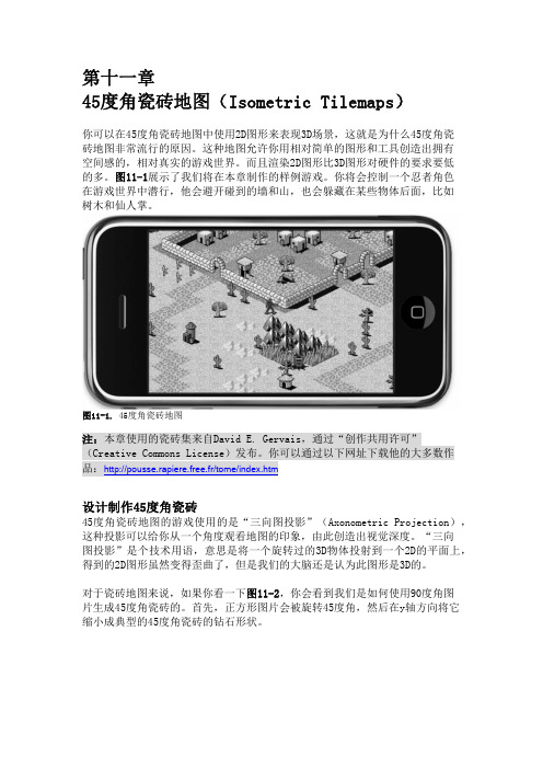
图11-1. 45度角瓷砖地图
注:本章使用的瓷砖集来自David E. Gervais,通过“创作共用许可” (Creative Commons License)发布。你可以通过以下网址下载他的大多数作 品:http://pousse.rapiere.free.fr/tome/index.htm
设计制作45度角瓷砖
打开Tiled软件,选择File > New菜单会出现如图11-7所示的 New Map 对话框。 显然,Orientation 应该被设置为 Isometric,Map size 的width(宽度)和 height(高度)设为30块瓷砖。比较奇怪的一个设置是Tile size的宽度和高度 设置。之前我提到过dg_iso32.png中的单块瓷砖的大小是 54x49 像素。而钻石 形状的大小(当你将瓷砖放到地图中时,你要考虑这个尺寸)是 54x27 像素。 但是我们在这里设置的却是 52x26 像素。
depthmap空间句法

depthmap空间句法深度图空间句法(DepthmapSpaceSyntax,以下简称DSS)是一种新型的超级句法方法(Super Syntax Method,以下简称SSM),用于分析和理解句子中的语义关系。
它不仅可以将文本分析为语义元素(如宾语、定语等),而且还能分析其空间表示。
它是一种非常强大的自然语言处理工具,能够有效地构建复杂句子中的语义关系,从而分析出句子的含义。
DSS是一种基于句子分析的自然语言处理方法,也就是基于空间表示的方法,它的一个重要特点是能够有效地处理复杂的句法结构,这些句法结构表示语义关系。
它通过一种叫做深度图的画法将句子分解成多层次的句子元素,然后把这些元素组合起来构成一个半结构化的句子空间,这种句子空间被称为深度图空间(Depthmap Space,以下简称DS)。
这个深度图空间里的元素可以表示句子的空间关系,包括句子内部和句子间的关系。
DSS的主要思想是通过深度图空间分析,分析句子中的语义关系,从而研究语义关系的空间表征。
在DSS的结构中,每个句子都是一个深度图,由语义元素构成。
空间表示的每一层都包含一些句子内部的关系,以及与句子之间间接关系,这样就可以建立起一个半结构化的句子空间,使一句话能够更好地表示其意义。
DSS与传统句法的不同之处在于它处理的是句子的空间表示,而传统句法是处理句子的层次表示。
在DSS中,每个句子将被分解成多个语义元素,而传统句法则是将句子分解成语法角色。
这样,DSS可以更深入地分析句子,如宾语、定语、修饰词等,并将它们排列组合,从而分析句子的空间表示,使其具有完整的语义结构和深度推理。
DSS也具有许多有用的应用,比如机器翻译、文本分类和问答系统等。
在机器翻译中,它可以有效地处理复杂的语法,给出更准确的翻译结果;在文本分类中,它可以帮助自然语言处理系统更好地分析文本,从而更加准确地进行文本分类;在问答系统中,它可以更加准确地理解句子的意思,从而建立起一个更准确的问答系统。
密集匹配
摘要计算机视觉中获得一个场景的三维信息,是一个从二维信息推算三维信息的过程。
而影像的密集匹配是整个三维恢复过程中最为重要的一个步骤,通过密集匹配,获得所有像素点准确的深度信息,从而完成三维重建。
在计算机视觉中,通常为了获取一个目标更加丰富与详细的信息,对同一场景往往将从不同的角度拍摄,从而得到该场景多个不同的视角,称之为多视角影像。
相比较于一般影像,多视角影像存在着宽基线,变形大,遮挡严重的特点,因此给密集匹配造成较大的困难。
本文即针对多视角影像,在总结前人的工作基础上,提出一种新的密集匹配的方法。
该方法的核心在于进行稀疏匹配时使用DAISY算法对特征点进行描述,从而很大程度上提高了效率,为了进一步提高效率,使用了SURF特征提取算子以及k-d树的匹配方法,同时为了保证匹配的正确性,利用RANSAC方法估计基础矩阵,进行极线约束。
最后,通过前方交会得到较为密集的三维点云,利用RBF算法进行内插得到目标物体的三维表面模型。
关键词:多视角密集匹配;特征提取;三维重建ABSTRACTThe process of obtaining three dimensional information from a scene in Computer Vision is also a process of calculating three dimensional information from two dimensional information. Dense Matching of images is the most important step in the process of 3D Recovery. Through Dense Matching, we could get accurate depth information of all pixels and achieve the purpose of rebuilding.In Computer Vision, we usually shoot the same scene from different perspectives in order to get more abundant and detailed information of the object. And then, we can obtain several different perspectives of the scene, which we call it multi-view image. Compared with general images, multi-view image has wide baseline, large deformation and is always seriously sheltered, which creates great difficulties for Dense Matching.Based on summarizing predecessors’ work, I put forward a new method for Dense Matching, and aiming at better handling the multi-view images. The heart of the method is using DAISY algorithm to describe the feature points during Sparse Matching. This greatly improve the efficiency of matching. In order to further raise the efficiency, I also add SURF feature extraction operator and the matching method of kd-tree. At the same time, I adopt RANSAC method to estimate basic matrix and complete polar constraint to ensure the correctness of the matching. Finally, I get dense 3D point cloud through forward intersection, and establish the object’s 3D surface model through the RBF algorithm for interpolation.Key words: Multi-view Dense Matching; Pattern Extraction; 3D Reconstruction目录第1章绪论1.1 研究背景及意义 (1)1.2 国内外研究现状 (2)1.3 本文研究思路 (4)第2章密集匹配相关理论和算法基础2.1 特征匹配算法基础 (6)2.1.1 SURF特征点提取原理 (6)2.1.2 DAISY描述符算法原理 (10)2.1.3 kd树匹配原理 (13)2.3 误匹配剔除算法基础 (15)2.3.1 极几何以及基本矩阵介绍 (15)2.3.2 RANSAC算法原理 (19)2.4 三维重建原理 (20)2.4.1 三角原理 (20)2.4.2 RBF内插算法介绍 (21)第3章基于DAISY的多视角密集匹配算法3.1 特征提取和描述 (24)3.1.1 特征提取 (24)3.1.2 DAISY算法进行描述 (26)3.2 影像匹配 (28)3.2.1 立体像对匹配实现 (28)3.2.2 多视角影像匹配实现 (31)3.3 三维恢复 (31)第4章实验结果与分析4.1 实验数据 (34)4.2 密集匹配实验结果 (36)4.2.1 立体像对密集匹配实验 (36)4.2.2 多视角密集匹配结果...................................................错误!未定义书签。
SpaceSyntax【空间句法】之DepthMapX学习:第二篇输出了什么东西与核心概念

SpaceSyntax【空间句法】之DepthMapX学习:第⼆篇输出了什么东西与核⼼概念这节⽐较枯燥,都是原理,不过也有⼲货。
这篇能不能听懂,就决定是否⼊门...所以,加油吧博客园/B站/知乎/CSDN @秋意正寒转载请在⽂头注明本⽂地址本篇讲空间句法的⼏个核⼼概念,有⼀些也是重要的分析结果(在DepthMapX中,作为某个分析图层的属性返回,具体见后⾯的博客,有介绍如何操作、导出结果)本系列⽬录:以下所有的属性,除了VGA,都是某⼀个轴线/线段/凸多边形的⼀个属性值,如整合度是1.34是对于某个轴线⽽⾔的。
1. 连通性(Conectivity属性)连通性代表这个元素与⼏个元素相连接。
2. 拓扑深度(Topological Depth属性)——描述深度拓扑深度在概念上⽐较拗⼝,个⼈总结为:。
⽐如,你家有地下五层,第五层还有⼀个秘密隧道,隧道尽头有个秘密房间,⾥⾯放满了很多箱⼦,你的满⽉照⽚就放在最⾥头的⼀个箱⼦⾥⾯的⼀本字典中的某⼀页夹层——这个“深度”够不够真实?总之,拓扑深度(有时⼜叫全局拓扑深度,简写 Total Depth即TD)是⼀个负向指标,,说明这个元素。
3. 整合度(Integration属性)——描述通达能⼒整合度是根据上⾯拓扑深度TD值经过⼀系列标准化计算后,得到的⼀个正向指标。
具体的公式我会在下⽅贴出来。
它和拓扑深度是反⽐关系——拓扑深度越⾼,整合度越低;拓扑深度越低,整合度越⾼。
很简单,上⾯说“拓扑深度越⼤,反过来意思就是整合度越⼩”的⼀个元素,它藏得越深,可访问性就越低,就越不⽅便去到那⾥——⽐如死胡同。
所以我们认为,在某种意义上,拓扑深度越⼤(地⽅越偏僻)的地⽅,整合度(让⼈想去的欲望)越⼩。
倘若有兴趣,可以看看整合度如何由拓扑深度TD值推演⽽来。
4. 选择度(Choice属性)——描述路过的概率选择度是⼀个正向指标,它代表的含义是当前元素的“被路过”的可能性,也就是穿越能⼒。
第十一章_深度图
第十一章深度图获取场景中各点相对于摄象机的距离是计算机视觉系统的重要任务之一.场景中各点相对于摄象机的距离可以用深度图(Depth Map)来表示,即深度图中的每一个像素值表示场景中某一点与摄像机之间的距离.机器视觉系统获取场景深度图技术可分为被动测距传感和主动深度传感两大类.被动测距传感是指视觉系统接收来自场景发射或反射的光能量,形成有关场景光能量分布函数,即灰度图像,然后在这些图像的基础上恢复场景的深度信息.最一般的方法是使用两个相隔一定距离的摄像机同时获取场景图像来生成深度图.与此方法相类似的另一种方法是一个摄象机在不同空间位置上获取两幅或两幅以上图像,通过多幅图像的灰度信息和成象几何来生成深度图.深度信息还可以使用灰度图像的明暗特征、纹理特征、运动特征间接地估算.主动测距传感是指视觉系统首先向场景发射能量,然后接收场景对所发射能量的反射能量.主动测距传感系统也称为测距成象系统(Rangefinder).雷达测距系统和三角测距系统是两种最常用的两种主动测距传感系统.因此,主动测距传感和被动测距传感的主要区别在于视觉系统是否是通过增收自身发射的能量来测距。
另外,我们还接触过两个概念:主动视觉和被动视觉。
主动视觉是一种理论框架,与主动测距传感完全是两回事。
主动视觉主要是研究通过主动地控制摄象机位置、方向、焦距、缩放、光圈、聚散度等参数,或广义地说,通过视觉和行为的结合来获得稳定的、实时的感知。
我们将在最后一节介绍主动视觉。
11.1 立体成象最基本的双目立体几何关系如图11.1(a)所示,它是由两个完全相同的摄象机构成,两个图像平面位于一个平面上,两个摄像机的坐标轴相互平行,且x轴重合,摄像机之间在x方向上的间距为基线距离b.在这个模型中,场景中同一个特征点在两个摄象机图像平面上的成象位置是不同的.我们将场景中同一点在两个不同图像中的投影点称为共轭对,其中的一个投影点是另一个投影点的对应(correspondence),求共轭对就是求解对应性问题.两幅图像重叠时的共轭对点的位置之差(共轭对点之间的距离)称为视差(disparity),通过135136 两个摄象机中心并且通过场景特征点的平面称为外极(epipolar)平面,外极平面与图像平面的交线称为外极线.在图11.1 中,场景点P 在左、右图像平面中的投影点分为p l 和p r .不失一般性,假设坐标系原点与左透镜中心重合.比较相似三角形PMC l 和p LC l l ,可得到下式:F x z x l '= (11.1) 同理,从相似三角形PNC r 和p RC l r ,可得到下式:Fx z B x r '=- (11.2) 合并以上两式,可得:r l x x BF z '-'= (11.3)其中F 是焦距,B 是基线距离。
opencv reprojectimageto3d得出三维点云的原理 -回复

opencv reprojectimageto3d得出三维点云的原理-回复Opencv中的reprojectImageTo3D函数是一个用于将二维图像上的点重新投影到三维空间中的函数。
通过该函数,可以从图像的深度信息中推断出每个像素点在三维空间中对应的坐标。
原理:1. 计算相机内参矩阵(Camera Intrinsic Matrix):在进行相机标定之后,可以得到相机的内参矩阵K。
相机内参矩阵包含了相机的焦距、光心等相关参数,它描述了相机在成像过程中的内部结构。
2. 计算相机的外参矩阵(Extrinsic Matrix):相机的外参矩阵描述了相机在世界坐标系下的位置和方向。
它包括了旋转矩阵R和平移矩阵t。
这些外参参数可以通过相机标定或者其他外部传感器获得。
3. 确定参考点(Reference Point):通过重建算法或者其他方式,确定一个已知的三维点(参考点)的坐标,作为后续计算的参考基准。
4. 获取图像的深度图(Depth Map):从深度传感器或者其他方法获取图像的深度信息。
深度图是一个灰度图像,每个像素点表示该点的距离或者深度值。
5. 根据图像的深度信息,计算每个像素点的三维坐标:reprojectImageTo3D函数根据相机的内参矩阵、外参矩阵以及图像的深度图,计算出每个像素点在相机坐标系下的三维坐标。
算法的基本原理是根据相机的焦距和光心位置,将像素坐标映射到归一化相机坐标系下,再通过深度信息将归一化相机坐标映射到三维坐标。
6. 进行坐标转换:将计算得到的三维坐标从相机坐标系转换到世界坐标系或其他参考坐标系下。
7. 可视化三维点云:将计算得到的三维坐标可视化为点云,可以使用OpenGL或者其他可视化工具进行展示。
该函数的基本原理如上所述,通过相机的内参矩阵、外参矩阵和深度图像,可以将二维图像上的点投影到三维空间中。
这对于立体视觉、三维重建等应用具有重要的意义。
然而,由于相机标定的误差、深度传感器的精度等因素的影响,reprojectImageTo3D函数在实际应用中可能存在一定的误差。
基于深度图的水下图像复原

第51卷第2期2021年3月吉林大学学报(工学版)Journal of Jilin University (Engineering and T e c h n o l o g y Edition)V ol. 51 N o. 2Mar. 2021基于深度图的水下图像复原郭继昌,乔珊珊(天津大学电气自动化与信息工程学院,天津300072)摘要:水下图像深度图估计的准确性影响复原后的图像质量,为得到更加准确的深度图,提 出了 一种基于衰减通道结合亮度图的深度图求解算法,并利用该深度图复原水下图像。
首先,根据图像像素值与场景深度的关系估计水下图像的深度图,并使用图像的亮度图对深度图进 行修正和细化;然后,利用深度图计算图像的大气光值和透射率图;最后,通过逆求解水下成像 模型复原退化的图像。
实验证明:与现有算法相比,利用该深度图得到的模型参数更加准确,复原后的图像不仅拥有更好的对比度,而且能保持自然真实的颜色。
关键词:信息处理技术;水下图像复原;水下成像模型;深度图中图分类号:T P391 文献标志码:A文章编号:1671-5497(2021)02-0677-08D O I:10. 13229/ki.j d x bgxb20191064Underwater image restoration based on depth mapG U O Ji~c h a n g,Q I A O Shan-shan{School of Electrical and Information Engineering ^Tianjin University ^Tianjin 300072, China)A b s t r a c t:T h e estimated accuracy of the depth m a p s of underwater images affects the quality of the restored i m a g e s.In order to obtain m o r e precise depth m a p s,an algorithm w a s proposed to calculate the depth m a p based on attenuated channels and luminance m a p,and then the depth m a p w a s used to recover underwater i m a g e s.First,the depth m a p of underwater image i s estimated according to the relationship b e t w e e n i m a g e pixel and scene depth.T h e n the depth m a p is further rectified a nd refined by using the luminance m a p. T h i r d,the atmospheric light value and the transmission m a p of the im a g e is calculated using the refined depth m a p.Finally,the degraded underwater im a g e i s restored b y inversely solving the underwater imaging m o d e l.T h e experimental results s h o w that c o m p a r e d with the existing algorithms,the m o d e l parameters calculated using the rectified depth m a p are m o r e accurate,and the restored i m a g e has better contrast and can maintain m o r e natural color.K e y w o r d s:information procevSsion technology;underwater im a g e restoration;underwater imaging m o d e l;depth m a p收稿日期:2019-11-21.基金项目:国家自然科学基金项目(61771334).作者简介:郭继昌(1966-),男,教授,博士 .研究方向:智能视频/图像分析,识别及处理.E-m a il:jcgU〇@•678•吉林大学学报(工学版)第51卷〇引言由于水下环境的特性,光在水下传播时会因为水中溶解的有机物以及悬浮颗粒等的存在而发 生散射,并且不同颜色的光,会由于波长不同受到 不同程度的衰减,所以水下图像会呈现出低对比度和严重的色彩偏移现象11:随着海洋资源的开发探索及计算机视觉的发展,水下图像清晰化技 术也受到了越来越多的关注124|。
- 1、下载文档前请自行甄别文档内容的完整性,平台不提供额外的编辑、内容补充、找答案等附加服务。
- 2、"仅部分预览"的文档,不可在线预览部分如存在完整性等问题,可反馈申请退款(可完整预览的文档不适用该条件!)。
- 3、如文档侵犯您的权益,请联系客服反馈,我们会尽快为您处理(人工客服工作时间:9:00-18:30)。
南京航空航天大学 自动化学院
6
立体成象的最一般情况:一个运动摄像机连续获取场 景图像,形成立体图像序列,或间隔一定距离的两个 摄像机同时获取场景图像,形成立体图像对。
南京航空航天大学 自动化学院
7
2. 立体匹配的基本方法
立体成象系统的一个不言而喻的假设是 能够找到立体图像对中的共轭对,即求解对 应问题.然而,对于实际的立体图像对,求 解对应问题极富有挑战性,可以说是立体视 觉最困难的一步.为了求解对应,人们已经 建立了许多约束来减少对应点搜索范围,并 最终确定正确的对应.
南京航空航天大学 自动化学院
14
考虑两幅图像 f1和 f2.设待匹配的候选特征点对的视差 为 (d x , d y ),则以特征点为中心的区域之间相似性测度可 由相关系数 r (d x , d y ) 定义为:
r (d x , d y )
{
( x , y )S
[ f1 ( x, y ) f1 ][ f 2 ( x d x , y d y ) f 2 ]
南京航空航天大学 自动化学院
11
(2)基于边缘的立体匹配
• 在某一行上计算各边缘的位置.
• 通过比较边缘的方向和强度粗略地进行边缘匹 配.
• 通过在精细尺度上进行匹配,可以得到视差估
计.
水平边缘无法进行匹配!
南京航空航天大学 自动化学院
12
(3)基于区域相关性的立体匹配
• 在立体图像对中识别兴趣点(interesting point),而后使 用区域相关法来匹配两幅图像中相对应的点.
南京航空航天大学 自动化学院 5
BF z xr xl
提高精度的措施是增大基线距离。产生的问题: 随着基线距离的增加,两个摄象机的共同的可视 范围减小;场景点对应的视差值增大,则搜索对 应点的范围增大,出现多义性的机会就增大;由 于透视投影引起的变形导致两个摄象机获取的两 幅图像中不完全相同,这就给确定共轭对带来了 i, j 0 ) / 0
f k i, j ( f k i, j k ) / k
f k i, j 是参考摄像机的图象函数
1 n m 2 ( f ( i , j ) ) m n j 1 i 1
南京航空航天大学 自动化学院 3
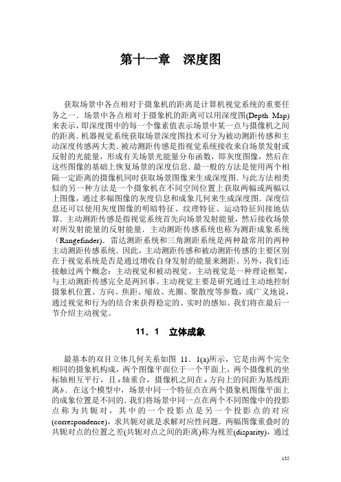
1.立体成像
• 外极平面 • 外极线 • 共轭对 • 视差 (disparity)
图11.1双目立体视觉几何模型
南京航空航天大学 自动化学院 4
假设坐标系原点与左透镜中 心重合。F是焦距,B是基线 距离。
x x l z F
x B xr z F
BF z xr xl
( x , y )S ( x , y )S
2 [ f ( x , y ) f ( x 1 , y 1 )] 2 [ f ( x , y ) f ( x 1 , y 1 )]
( x , y )S
I ( xc , yc ) min(I1, I 2 , I3 , I 4 )
2 [ f ( x , y ) f ] 1 ( x , y )S 1
2 1/ 2 [ f ( x d , y d ) f ] x y 2 } ( x , y )S 1
南京航空航天大学 自动化学院
2
•被动测距传感:视觉系统接收来自场景发射 或反射的光能量,形成有关场景光能量分布 函数,即灰度图像,然后在这些图像的基础 上恢复场景的深度信息.
•主动测距传感:视觉系统首先向场景发射能 量,然后接收场景对所发射能量的反射能 量.主动测距传感系统也称为测距成象系统 (Rangefinder).
南京航空航天大学 自动化学院 13
• 特征点匹配
一旦在两幅图像中确定特征后,则可以使用许 多不同方法进行特征匹配.一种简单的方法是计算 一幅图像以某一特征点为中心的一个小窗函数内的 像素与另一幅图像中各个潜在对应特征点为中心的 同样的小窗函数的像素之间的相关值.具有最大相 关值的特征就是匹配特征.很明显,只有满足外极 线约束的点才能是匹配点.考虑到垂直视差的存在, 应将外极线邻近的特征点也包括在潜在的匹配特征 集中.
第
11
章
深度图 (Depth Map)
南京航空航天大学 自动化学院
1
获取场景中各点相对于摄象机的距离 是计算机视觉系统的重要任务之一.场景 中各点相对于摄象机的距离可以用深度图 (Depth Map)来表示,即深度图中的每一 个像素值表示场景中某一点与摄像机之间 的距离.机器视觉系统获取场景深度图技 术可分为被动测距传感和主动测距传感两 大类.
南京航空航天大学 自动化学院
8
(1) 立体匹配的基本约束 • 外极线约束
图11.4 空间某一距离区间内的一条直线段对应外极线上的一个有限区 间
南京航空航天大学 自动化学院 9
•一致性约束
立体视觉通常由两个或两个以上摄像机组成,各摄像机的 特性一般是不同的.这样,场景中对应点处的光强可能相差太 大,直接进行相似性匹配,得到的匹配值变化太大.因此,在 进行匹配前,必须对图像进行规范化处理(Normalization).
• 兴趣点计算公式如下:
在以某一点为中心 的窗函数中,计算 其在不同方向上的 变化量是这些方向 上点的差异性的最 好测度。S表示窗函 数中的所有像素 。
I1 I2 I3 I4
( x , y )S 2 [ f ( x , y ) f ( x , y 1 )] 2 [ f ( x , y ) f ( x 1 , y )]
2
相似估价函数: k
f
i 1 j 1
n
m
0
(i, j ) f k (i, j )
10
南京航空航天大学 自动化学院
• 唯一性约束:一般情况下,一幅图像(左或右)上的 每一个特征点只能与另一幅图像上的唯一一个特征 对应。 • 连续性约束:物体表面一般都是光滑的,因此物 体表面上各点在图像上的投影也是连续的,它们的 视差也是连续的.比如,物体上非常接近的两点, 其视差也十分接近,因为其深度值不会相差很大。