数据库系统基础教程第二章复习资料
数据库系统基础教程(第二版)课后习题答案2
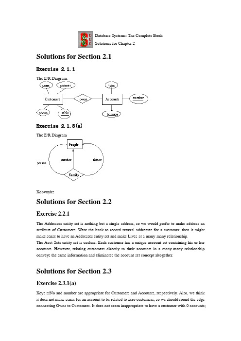
Database Systems: The Complete BookSolutions for Chapter 2Solutions for Section 2.1Exercise 2.1.1The E/R Diagram.Exercise 2.1.8(a)The E/R DiagramKobvxybzSolutions for Section 2.2Exercise 2.2.1The Addresses entity set is nothing but a single address, so we would prefer to make address an attribute of Customers. Were the bank to record several addresses for a customer, then it might make sense to have an Addresses entity set and make Lives-at a many-many relationship.The Acct-Sets entity set is useless. Each customer has a unique account set containing his or her accounts. However, relating customers directly to their accounts in a many-many relationship conveys the same information and eliminates the account-set concept altogether.Solutions for Section 2.3Exercise 2.3.1(a)Keys ssNo and number are appropriate for Customers and Accounts, respectively. Also, we think it does not make sense for an account to be related to zero customers, so we should round the edge connecting Owns to Customers. It does not seem inappropriate to have a customer with 0 accounts;they might be a borrower, for example, so we put no constraint on the connection from Owns to Accounts. Here is the The E/R Diagram,showing underlined keys andthe numerocity constraint.Exercise 2.3.2(b)If R is many-one from E1 to E2, then two tuples (e1,e2) and (f1,f2) of the relationship set for R must be the same if they agree on the key attributes for E1. To see why, surely e1 and f1 are the same. Because R is many-one from E1 to E2, e2 and f2 must also be the same. Thus, the pairs are the same.Solutions for Section 2.4Exercise 2.4.1Here is the The E/R Diagram.We have omitted attributes other than our choice for the key attributes of Students and Courses. Also omitted are names for the relationships. Attribute grade is not part of the key for Enrollments. The key for Enrollements is studID from Students and dept and number from Courses.Exercise 2.4.4bHere is the The E/R Diagram Again, we have omitted relationship names and attributes other than our choice for the key attributes. The key for Leagues is its own name; this entity set is not weak. The key for Teams is its own name plus the name of the league of which the team is a part, e.g., (Rangers, MLB) or (Rangers, NHL). The key for Players consists of the player's number and the key for the team on which he or she plays. Since the latter key is itself a pair consisting of team and league names, the key for players is the triple (number, teamName, leagueName). e.g., JeffGarcia is (5, 49ers, NFL).Database Systems: The Complete BookSolutions for Chapter 3Solutions for Section 3.1Exercise 3.1.2(a)We can order the three tuples in any of 3! = 6 ways. Also, the columns can be ordered in any of 3! = 6 ways. Thus, the number of presentations is 6*6 = 36.Solutions for Section 3.2Exercise 3.2.1Customers(ssNo, name, address, phone)Flights(number, day, aircraft)Bookings(ssNo, number, day, row, seat)Being a weak entity set, Bookings' relation has the keys for Customers and Flights and Bookings' own attributes.Notice that the relations obtained from the toCust and toFlt relationships are unnecessary. They are:toCust(ssNo, ssNo1, number, day)toFlt(ssNo, number, day, number1, day1)That is, for toCust, the key of Customers is paired with the key for Bookings. Since both include ssNo, this attribute is repeated with two different names, ssNo and ssNo1. A similar situation exists for toFlt.Exercise 3.2.3Ships(name, yearLaunched)SisterOf(name, sisterName)Solutions for Section 3.3Exercise 3.3.1Since Courses is weak, its key is number and the name of its department. We do not have arelation for GivenBy. In part (a), there is a relation for Courses and a relation for LabCourses that has only the key and the computer-allocation attribute. It looks like:Depts(name, chair)Courses(number, deptName, room)LabCourses(number, deptName, allocation)For part (b), LabCourses gets all the attributes of Courses, as:Depts(name, chair)Courses(number, deptName, room)LabCourses(number, deptName, room, allocation)And for (c), Courses and LabCourses are combined, as:Depts(name, chair)Courses(number, deptName, room, allocation)Exercise 3.3.4(a)There is one relation for each entity set, so the number of relations is e. The relation for the root entity set has a attributes, while the other relations, which must include the key attributes, have a+k attributes.Solutions for Section 3.4Exercise 3.4.2Surely ID is a key by itself. However, we think that the attributes x, y, and z together form another key. The reason is that at no time can two molecules occupy the same point.Exercise 3.4.4The key attributes are indicated by capitalization in the schema below:Customers(SSNO, name, address, phone)Flights(NUMBER, DAY, aircraft)Bookings(SSNO, NUMBER, DAY, row, seat)Exercise 3.4.6(a)The superkeys are any subset that contains A1. Thus, there are 2^{n-1} such subsets, since each of the n-1 attributes A2 through An may independently be chosen in or out.Solutions for Section 3.5Exercise 3.5.1(a)We could try inference rules to deduce new dependencies until we are satisfied we have them all.A more systematic way is to consider the closures of all 15 nonempty sets of attributes.For the single attributes we have A+ = A, B+ = B, C+ = ACD, and D+ = AD. Thus, the only new dependency we get with a single attribute on the left is C->A.Now consider pairs of attributes:AB+ = ABCD, so we get new dependency AB->D. AC+ = ACD, and AC->D is nontrivial. AD+ = AD, so nothing new. BC+ = ABCD, so we get BC->A, and BC->D. BD+ = ABCD, giving usBD->A and BD->C. CD+ = ACD, giving CD->A.For the triples of attributes, ACD+ = ACD, but the closures of the other sets are each ABCD. Thus, we get new dependencies ABC->D, ABD->C, and BCD->A.Since ABCD+ = ABCD, we get no new dependencies.The collection of 11 new dependencies mentioned above is: C->A, AB->D, AC->D, BC->A, BC->D, BD->A, BD->C, CD->A, ABC->D, ABD->C, and BCD->A.Exercise 3.5.1(b)From the analysis of closures above, we find that AB, BC, and BD are keys. All other sets either do not have ABCD as the closure or contain one of these three sets.Exercise 3.5.1(c)The superkeys are all those that contain one of those three keys. That is, a superkey that is not a key must contain B and more than one of A, C, and D. Thus, the (proper) superkeys are ABC, ABD, BCD, and ABCD.Exercise 3.5.3(a)We must compute the closure of A1A2...AnC. Since A1A2...An->B is a dependency, surely B is in this set, proving A1A2...AnC->B.Exercise 3.5.4(a)Consider the relationThis relation satisfies A->B but does not satisfy B->A.Exercise 3.5.8(a)If all sets of attributes are closed, then there cannot be any nontrivial functional dependenc ies. For suppose A1A2...An->B is a nontrivial dependency. Then A1A2...An+ contains B and thus A1A2...An is not closed.Exercise 3.5.10(a)We need to compute the closures of all subsets of {ABC}, although there is no need to think about the empty set or the set of all three attributes. Here are the calculations for the remaining six sets: A+ = AB+ = BC+ = ACEAB+ = ABCDEAC+ = ACEBC+ = ABCDEWe ignore D and E, so a basis for the resulting functional dependencies for ABC are: C->A and AB->C. Note that BC->A is true, but follows logically from C->A, and therefore may be omitted from our list.Solutions for Section 3.6Exercise 3.6.1(a)In the solution to Exercise 3.5.1 we found that there are 14 nontrivial dependencies, including the three given ones and 11 derived dependencies. These are: C->A, C->D, D->A, AB->D, AB-> C, AC->D, BC->A, BC->D, BD->A, BD->C, CD->A, ABC->D, ABD->C, and BCD->A.We also learned that the three keys were AB, BC, and BD. Thus, any dependency above that does not have one of these pairs on the left is a BCNF violation. These are: C->A, C->D, D->A, AC->D, and CD->A.One choice is to decompose using C->D. That gives us ABC and CD as decomposed relations. CD is surely in BCNF, since any two-attribute relation is. ABC is not in BCNF, since AB and BC are its only keys, but C->A is a dependency that holds in ABCD and therefore holds in ABC. We must further decompose ABC into AC and BC. Thus, the three relations of the decomposition are AC, BC, and CD.Since all attributes are in at least one key of ABCD, that relation is already in 3NF, and no decomposition is necessary.Exercise 3.6.1(b)(Revised 1/19/02) The only key is AB. Thus, B->C and B->D are both BCNF violations. The derived FD's BD->C and BC->D are also BCNF violations. However, any other nontrivial, derived FD will have A and B on the left, and therefore will contain a key.One possible BCNF decomposition is AB and BCD. It is obtained starting with any of the four violations mentioned above. AB is the only key for AB, and B is the only key for BCD.Since there is only one key for ABCD, the 3NF violations are the same, and so is the decomposition.Solutions for Section 3.7Exercise 3.7.1Since A->->B, and all the tuples have the same value for attribute A, we can pair the B-value from any tuple with the value of the remaining attribute C from any other tuple. Thus, we know that R must have at least the nine tuples of the form (a,b,c), where b is any of b1, b2, or b3, and c is any of c1, c2, or c3. That is, we can derive, using the definition of a multivalued dependency, that each of the tuples (a,b1,c2), (a,b1,c3), (a,b2,c1), (a,b2,c3), (a,b3,c1), and (a,b3,c2) are also in R.Exercise 3.7.2(a)First, people have unique Social Security numbers and unique birthdates. Thus, we expect the functional dependencies ssNo->name and ssNo->birthdate hold. The same applies to children, so we expect childSSNo->childname and childSSNo->childBirthdate. Finally, an automobile has a unique brand, so we expect autoSerialNo->autoMake.There are two multivalued dependencies that do not follow from these functional dependencies. First, the information about one child of a person is independent of other information about that person. That is, if a person with social security number s has a tuple with cn,cs,cb, then if there isany other tuple t for the same person, there will also be another tuple that agrees with t except that it has cn,cs,cb in its components for the child name, Social Security number, and birthdate. That is the multivalued dependencyssNo->->childSSNo childName childBirthdateSimilarly, an automobile serial number and make are independent of any of the other attributes, so we expect the multivalued dependencyssNo->->autoSerialNo autoMakeThe dependencies are summarized below:ssNo -> name birthdatechildSSNo -> childName childBirthdateautoSerialNo -> autoMakessNo ->-> childSSNo childName childBirthdatessNo ->-> autoSerialNo autoMakeExercise 3.7.2(b)We suggest the relation schemas{ssNo, name, birthdate}{ssNo, childSSNo}{childSSNo, childName childBirthdate}{ssNo, autoSerialNo}{autoSerialNo, autoMake}An initial decomposition based on the two multivalued dependencies would give us {ssNo, name, birthDate}{ssNo, childSSNo, childName, childBirthdate}{ssNo, autoSerialNo, autoMake}Functional dependencies force us to decompose the second and third of these.Exercise 3.7.3(a)Since there are no functional dependencies, the only key is all four attributes, ABCD. Thus, each of the nontrvial multivalued dependencies A->->B and A->->C violate 4NF. We must separate out the attributes of these dependencies, first decomposing into AB and ACD, and then decomposing the latter into AC and AD because A->->C is still a 4NF violation for ACD. The final set of relations are AB, AC, and AD.Exercise 3.7.7(a)Let W be the set of attributes not in X, Y, or Z. Consider two tuples xyzw and xy'z'w' in the relation R in question. Because X ->-> Y, we can swap the y's, so xy'zw and xyz'w' are in R. Because X ->-> Z, we can take the pair of tuples xyzw and xyz'w' and swap Z's to get xyz'w and xyzw'. Similarly, we can take the pair xy'z'w' and xy'zw and swap Z's to get xy'zw' and xy'z'w.In conclusion, we started with tuples xyzw and xy'z'w' and showed that xyzw' and xy'z'w must also be in the relation. That is exactly the statement of the MVD X ->-> Y-union-Z. Note that the above statements all make sense even if there are attributes in common among X, Y, and Z.Exercise 3.7.8(a)Consider a relation R with schema ABCD and the instance with four tuples abcd, abcd', ab'c'd, and ab'c'd'. This instance satisfies the MVD A->-> BC. However, it does not satisfy A->-> B. For example, if it did satisfy A->-> B, then because the instance contains the tuples abcd and ab'c'd, we would expect it to contain abc'd and ab'cd, neither of which is in the instance.Database Systems: The Complete BookSolutions for Chapter 4Solutions for Section 4.2Exercise 4.2.1class Customer {attribute string name;attribute string addr;attribute string phone;attribute integer ssNo;relationship Set<Account> ownsAcctsinverse Account::ownedBy;}class Account {attribute integer number;attribute string type;attribute real balance;relationship Set<Customer> ownedByinverse Customer::ownsAccts}Exercise 4.2.4class Person {attribute string name;relationship Person motherOfinverse Person::childrenOfFemalerelationship Person fatherOfinverse Person::childrenOfMalerelationship Set<Person> childreninverse Person::parentsOfrelationship Set<Person> childrenOfFemaleinverse Person::motherOfrelationship Set<Person> childrenOfMaleinverse Person::fatherOfrelationship Set<Person> parentsOfinverse Person::children}Notice that there are six different relationships here. For example, the inverse of the relationship that connects a person to their (unique) mother is a relationship that connects a mother (i.e., a female person) to the set of her children. That relationship, which we call childrenOfFemale, is different from the children relationship, which connects anyone -- male or female -- to their children.Exercise 4.2.7A relationship R is its own inverse if and only if for every pair (a,b) in R, the pair (b,a) is also in R. In the terminology of set theory, the relation R is ``symmetric.''Solutions for Section 4.3Exercise 4.3.1We think that Social Security number should me the key for Customer, and account number should be the key for Account. Here is the ODL solution with key and extent declarations.class Customer(extent Customers key ssNo){attribute string name;attribute string addr;attribute string phone;attribute integer ssNo;relationship Set<Account> ownsAcctsinverse Account::ownedBy;}class Account(extent Accounts key number){attribute integer number;attribute string type;attribute real balance;relationship Set<Customer> ownedByinverse Customer::ownsAccts}Solutions for Section 4.4Exercise 4.4.1(a)Since the relationship between customers and accounts is many-many, we should create a separate relation from that relationship-pair.Customers(ssNo, name, address, phone)Accounts(number, type, balance)CustAcct(ssNo, number)Exercise 4.4.1(d)Ther is only one attribute, but three pairs of relationships from Person to itself. Since motherOf and fatherOf are many-one, we can store their inverses in the relation for Person. That is, for each person, childrenOfMale and childrenOfFemale will indicate that persons's father and mother. The children relationship is many-many, and requires its own relation. This relation actually turns out to be redundant, in the sense that its tuples can be deduced from the relationships stored with Person. The schema:Persons(name, childrenOfFemale, childrenOfMale)Parent-Child(parent, child)Exercise 4.4.4Y ou get a schema like:Studios(name, address, ownedMovie)Since name -> address is the only FD, the key is {name, ownedMovie}, and the FD has a left side that is not a superkey.Exercise 4.4.5(a,b,c)(a) Struct Card { string rank, string suit };(b) class Hand {attribute Set theHand;};For part (c) we have:Hands(handId, rank, suit)Notice that the class Hand has no key, so we need to create one: handID. Each hand has, in the relation Hands, one tuple for each card in the hand.Exercise 4.4.5(e)Struct PlayerHand { string Player, Hand theHand };class Deal {attribute Set theDeal;}Alternatively, PlayerHand can be defined directly within the declaration of attribute theDeal. Exercise 4.4.5(h)Since keys for Hand and Deal are lacking, a mechanical way to design the database schema is to have one relation connecting deals and player-hand pairs, and another to specify the contents of hands. That is:Deals(dealID, player, handID)Hands(handID, rank, suit)However, if we think about it, we can get rid of handID and connect the deal and the player directly to the player's cards, as:Deals(dealID, player, rank, suit)Exercise 4.4.5(i)First, card is really a pair consisting of a suit and a rank, so we need two attributes in a relation schema to represent cards. However, much more important is the fact that the proposed schema does not distinguish which card is in which hand. Thus, we need another attribute that indicates which hand within the deal a card belongs to, something like:Deals(dealID, handID, rank, suit)Exercise 4.4.6(c)Attribute b is really a bag of (f,g) pairs. Thus, associated with each a-value will be zero or more (f,g) pairs, each of which can occur several times. We shall use an attribute count to indicate the number of occurrences, although if relations allow duplicate tuples we could simply allow duplicate (a,f,g) triples in the relation. The proposed schema is:C(a, f, g, count)Solutions for Section 4.5Exercise 4.5.1(b)Studios(name, address, movies{(title, year, inColor, length,stars{(name, address, birthdate)})})Since the information about a star is repeated once for each of their movies, there is redundancy. To eliminate it, we have to use a separate relation for stars and use pointers from studios. That is: Stars(name, address, birthdate)Studios(name, address, movies{(title, year, inColor, length,stars{*Stars})})Since each movie is owned by one studio, the information about a movie appears in only one tuple of Studios, and there is no redundancy.Exercise 4.5.2Customers(name, address, phone, ssNo, accts{*Accounts})Accounts(number, type, balance, owners{*Customers})Solutions for Section 4.6Exercise 4.6.1(a)We need to add new nodes labeled George Lucas and Gary Kurtz. Then, from the node sw (which represents the movie Star Wars), we add arcs to these two new nodes, labeled direc tedBy and producedBy, respectively.Exercise 4.6.2Create nodes for each account and each customer. From each customer node is an arc to a node representing the attributes of the customer, e.g., an arc labeled name to the customer's name. Likewise, there is an arc from each account node to each attribute of that account, e.g., an arc labeled balance to the value of the balance.To represent ownership of accounts by customers, we place an arc labeled owns from each customer node to the node of each account that customer holds (possibly jointly). Also, we placean arc labeled ownedBy from each account node to the customer node for each owner of that account.Exercise 4.6.5In the semistructured model, nodes represent data elements, i.e., entities rather than entity sets. In the E/R model, nodes of all types represent schema elements, and the data is not represented at all. Solutions for Section 4.7Exercise 4.7.1(a)<STARS-MOVIES><STAR starId = "cf" starredIn = "sw, esb, rj"><NAME>Carrie Fisher</NAME><ADDRESS><STREET>123 Maple St.</STREET><CITY>Hollywood</CITY></ADDRESS><ADDRESS><STREET>5 Locust Ln.</STREET><CITY>Malibu</CITY></ADDRESS></STAR><STAR starId = "mh" starredIn = "sw, esb, rj"><NAME>Mark Hamill</NAME><ADDRESS><STREET>456 Oak Rd.<STREET><CITY>Brentwood</CITY></ADDRESS></STAR><STAR starId = "hf" starredIn = "sw, esb, rj, wit"><NAME>Harrison Ford</NAME><ADDRESS><STREET>whatever</STREET><CITY>whatever</CITY></ADDRESS></STAR><MOVIE movieId = "sw" starsOf = "cf, mh"><TITLE>Star Wars</TITLE><YEAR>1977</YEAR></MOVIE><MOVIE movieId = "esb" starsOf = "cf, mh"><TITLE>Empire Strikes Back</TITLE><YEAR>1980</YEAR></MOVIE><MOVIE movieId = "rj" starsOf = "cf, mh"><TITLE>Return of the Jedi</TITLE><YEAR>1983</YEAR></MOVIE><MOVIE movieID = "wit" starsOf = "hf"><TITLE>Witness</TITLE><YEAR>1985</YEAR></MOVIE></STARS-MOVIES>Exercise 4.7.2<!DOCTYPE Bank [<!ELEMENT BANK (CUSTOMER* ACCOUNT*)><!ELEMENT CUSTOMER (NAME, ADDRESS, PHONE, SSNO)> <!A TTLIST CUSTOMERcustId IDowns IDREFS><!ELEMENT NAME (#PCDA TA)><!ELEMENT ADDRESS (#PCDA TA)><!ELEMENT PHONE (#PCDA TA)><!ELEMENT SSNO (#PCDA TA)><!ELEMENT ACCOUNT (NUMBER, TYPE, BALANCE)><!A TTLIST ACCOUNTacctId IDownedBy IDREFS><!ELEMENT NUMBER (#PCDA TA)><!ELEMENT TYPE (#PCDA TA)><!ELEMENT BALANCE (#PCDA TA)>]>Database Systems: The CompleteBookSolutions for Chapter 5Solutions for Section 5.2Exercise 5.2.1(a)PI_model( SIGMA_{speed >= 1000} ) (PC)Exercise 5.2.1(f)The trick is to theta-join PC with itself on the condition that the hard disk sizes are equal. That gives us tuples that have two PC model numbers with the same value of hd. However, these two PC's could in fact be the same, so we must also require in the theta-join that the model numbers be unequal. Finally, we want the hard disk sizes, so we project onto hd.The expression is easiest to see if we write it using some temporary values. We start by renaming PC twice so we can talk about two occurrences of the same attributes.R1 = RHO_{PC1} (PC)R2 = RHO_{PC2} (PC)R3 = R1 JOIN_{PC1.hd = PC2.hd AND PC1.model <> PC2.model} R2R4 = PI_{PC1.hd} (R3)Exercise 5.2.1(h)First, we find R1, the model-speed pairs from both PC and Laptop. Then, we find from R1 those computers that are ``fast,'' at least 133Mh. At the same time, we join R1 with Product to connect model numbers to their manufacturers and we project out the speed to get R2. Then we join R2 with itself (after renaming) to find pairs of different models by the same maker. Finally, we get our answer, R5, by projecting onto one of the maker attributes. A sequence of steps giving the desired expression is: R1 = PI_{model,speed} (PC) UNION PI_{model,speed} (Laptop)R2 = PI_{maker,model} (SIGMA_{speed>=700} (R1) JOIN Product)R3 = RHO_{T(maker2, model2)} (R2)R4 = R2 JOIN_{maker = maker2 AND model <> model2} (R3)R5 = PI_{maker} (R4)Exercise 5.2.2Here are figures for the expression trees of Exercise 5.2.1 Part (a)Part (f)Part (h). Note that the third figure is not really a tree, since it uses a common subexpression. We could duplicate the nodes to make it a tree, but using common subexpressions is a valuable form of query optimization. One of the benefits one gets from constructing ``trees'' for queries is the ability to combine nodes that represent common subexpressions.Exercise 5.2.7The relation that results from the natural join has only one attribute from each pair of equated attributes. The theta-join has attributes for both, and their columns are identical.Exercise 5.2.9(a)If all the tuples of R and S are different, then the union has n+m tuples, and this number is the maximum possible.The minimum number of tuples that can appear in the result occurs if every tuple of one relation also appears in the other. Surely the union has at least as many tuples as the larger of R and that is, max(n,m) tuples. However, it is possible for every tuple of the smaller to appear in the other, so it is possible that there are as few as max(n,m) tuples in the union.Exercise 5.2.10In the following we use the name of a relation both as its instance (set of tuples) and as its schema (set of attributes). The context determines uniquely which is meant.PI_R(R JOIN S) Note, however, that this expression works only for sets; it does not preserve the multipicity of tuples in R. The next two expressions work for bags.R JOIN DELTA(PI_{R INTERSECT S}(S)) In this expression, each projection of a tuple from S onto the attributes that are also in R appears exactly once in the second argument of the join, so it preserves multiplicity of tuples in R, except for those thatdo not join with S, which disappear. The DELTA operator removes duplicates, as described in Section 5.4.R - [R - PI_R(R JOIN S)] Here, the strategy is to find the dangling tuples of R and remove them.Solutions for Section 5.3Exercise 5.3.1As a bag, the value is {700, 1500, 866, 866, 1000, 1300, 1400, 700, 1200, 750, 1100, 350, 733}. The order is unimportant, of course. The average is 959.As a set, the value is {700, 1500, 866, 1000, 1300, 1400, 1200, 750, 1100, 350, 733}, and the average is 967. H3>Exercise 5.3.4(a)As sets, an element x is in the left-side expression(R UNION S) UNION Tif and only if it is in at least one of R, S, and T. Likewise, it is in the right-side expressionR UNION (S UNION T)under exactly the same conditions. Thus, the two expressions have exactly the same members, and the sets are equal.As bags, an element x is in the left-side expression as many times as the sum of the number of times it is in R, S, and T. The same holds for the right side. Thus, as bags the expressions also have the same value.Exercise 5.3.4(h)As sets, element x is in the left sideR UNION (S INTERSECT T)if and only if x is either in R or in both S and T. Element x is in the right side(R UNION S) INTERSECT (R UNION T)if and only if it is in both R UNION S and R UNION T. If x is in R, then it is in both unions. If x is in both S and T, then it is in both union. However, if x is neither in R nor in both of S and T, then it cannot be in both unions. For example, suppose x is not in R and not in S. Then x is not in R UNION S. Thus, the statement of when x is in the right side is exactly the same as when it is in the left side: x is either in R or in both of S and T.Now, consider the expression for bags. Element x is in the left side the sum of the number of times it is in R plus the smaller of the number of times x is in S and the number of times x is in T. Likewise, the number of times x is in the right side is the smaller ofThe sum of the number of times x is in R and in S.The sum of the number of times x is in R and in T.A moment's reflection tells us that this minimum is the sum of the number of times x is in R plus the smaller of the number of times x is in S and in T, exactly as for the left side.Exercise 5.3.5(a)For sets, we observe that element x is in the left side(R INTERSECT S) - T。
(完整版)数据库系统基础教程第二章答案解析

For relation Accounts, the attributes are:acctNo, type, balanceFor relation Customers, the attributes are:firstName, lastName, idNo, accountExercise 2.2.1bFor relation Accounts, the tuples are:(12345, savings, 12000),(23456, checking, 1000),(34567, savings, 25)For relation Customers, the tuples are:(Robbie, Banks, 901-222, 12345),(Lena, Hand, 805-333, 12345),(Lena, Hand, 805-333, 23456)Exercise 2.2.1cFor relation Accounts and the first tuple, the components are:123456 → acctNosavings → type12000 → balanceFor relation Customers and the first tuple, the components are:Robbie → firstNameBanks → lastName901-222 → idNo12345 → accountExercise 2.2.1dFor relation Accounts, a relation schema is:Accounts(acctNo, type, balance)For relation Customers, a relation schema is:Customers(firstName, lastName, idNo, account) Exercise 2.2.1eAn example database schema is:Accounts (acctNo,type,balance)Customers (firstName,lastName,idNo,account)A suitable domain for each attribute:acctNo → Integertype → Stringbalance → IntegerfirstName → StringlastName → StringidNo → String (because there is a hyphen we cannot use Integer)account → IntegerExercise 2.2.1gAnother equivalent way to present the Account relation:Another equivalent way to present the Customers relation:Exercise 2.2.2Examples of attributes that are created for primarily serving as keys in a relation:Universal Product Code (UPC) used widely in United States and Canada to track products in stores.Serial Numbers on a wide variety of products to allow the manufacturer to individually track each product.Vehicle Identification Numbers (VIN), a unique serial number used by the automotive industry to identify vehicles.Exercise 2.2.3aWe can order the three tuples in any of 3! = 6 ways. Also, the columns can be ordered in any of 3! = 6 ways. Thus, the number of presentations is 6*6 = 36.Exercise 2.2.3bWe can order the three tuples in any of 5! = 120 ways. Also, the columns can be ordered in any of 4! = 24 ways. Thus, the number of presentations is 120*24 = 2880Exercise 2.2.3cWe can order the three tuples in any of m! ways. Also, the columns can be ordered in any of n! ways. Thus, the number of presentations is n!m!Exercise 2.3.1aCREATE TABLE Product (maker CHAR(30),model CHAR(10) PRIMARY KEY,type CHAR(15));CREATE TABLE PC (model CHAR(30),speed DECIMAL(4,2),ram INTEGER,hd INTEGER,price DECIMAL(7,2));Exercise 2.3.1cCREATE TABLE Laptop (model CHAR(30),speed DECIMAL(4,2),ram INTEGER,hd INTEGER,screen DECIMAL(3,1),price DECIMAL(7,2));Exercise 2.3.1dCREATE TABLE Printer (model CHAR(30),color BOOLEAN,type CHAR (10),price DECIMAL(7,2));Exercise 2.3.1eALTER TABLE Printer DROP color;Exercise 2.3.1fALTER TABLE Laptop ADD od CHAR (10) DEFAULT ‘none’; Exercise 2.3.2aCREATE TABLE Classes (class CHAR(20),type CHAR(5),country CHAR(20),numGuns INTEGER,bore DECIMAL(3,1),displacement INTEGER);Exercise 2.3.2bCREATE TABLE Ships (name CHAR(30),class CHAR(20),launched INTEGER);Exercise 2.3.2cCREATE TABLE Battles (name CHAR(30),date DATE);Exercise 2.3.2dCREATE TABLE Outcomes (ship CHAR(30),battle CHAR(30),result CHAR(10));Exercise 2.3.2eALTER TABLE Classes DROP bore;Exercise 2.3.2fALTER TABLE Ships ADD yard CHAR(30); Exercise 2.4.1aR1 := σspeed ≥ 3.00 (PC)R2 := πmodel(R1)model100510061013Exercise 2.4.1bR1 := σhd ≥ 100 (Laptop)R2 := Product (R1)R3 := πmaker (R2)makerEABFGExercise 2.4.1cR1 := σmaker=B (Product PC)R2 := σmaker=B (Product Laptop)R3 := σmaker=B (Product Printer)R4 := πmodel,price (R1)R5 := πmodel,price (R2)R6: = πmodel,price (R3)R7 := R4 R5 R6model price1004 6491005 6301006 10492007 1429Exercise 2.4.1dR1 := σcolor = true AND type = laser (Printer)R2 := πmodel (R1)model30033007Exercise 2.4.1eR1 := σtype=laptop (Product)R2 := σtype=PC(Product)R3 := πmaker(R1)R4 := πmaker(R2)R5 := R3 – R4Exercise 2.4.1fR1 := ρPC1(PC)R2 := ρPC2(PC)R3 := R1 (PC1.hd = PC2.hd AND PC1.model <> PC2.model) R2R4 := πhd(R3)Exercise 2.4.1gR1 := ρPC1(PC)R2 := ρPC2(PC)R3 := R1 (PC1.speed = PC2.speed AND PC1.ram = PC2.ram AND PC1.model < PC2.model) R2R4 := πPC1.model,PC2.model(R3)Exercise 2.4.1hR1 := πmodel(σspeed ≥ 2.80(PC)) πmodel(σspeed ≥ 2.80(Laptop))R2 := πmaker,model(R1 Product)R3 := ρR3(maker2,model2)(R2)R4 := R2 (maker = maker2 AND model <> model2) R3R5 := πmaker(R4)Exercise 2.4.1iR1 := πmodel,speed(PC)R2 := πmodel,speed(Laptop)R3 := R1 R2R4 := ρR4(model2,speed2)(R3)R5 := πmodel,speed (R3 (speed < speed2 ) R4)R6 := R3 – R5makerBExercise 2.4.1jR1 := πmaker,speed(Product PC)R2 := ρR2(maker2,speed2)(R1)R3 := ρR3(maker3,speed3)(R1)R4 := R1 (maker = maker2 AND speed <> speed2) R2R5 := R4 (maker3 = maker AND speed3 <> speed2 AND speed3 <> speed) R3R6 := πmaker(R5)makerFGhd25080160PC1.model PC2.model1004 1012makerBEmakerADEExercise 2.4.1kR1 := πmaker,model(Product PC)R2 := ρR2(maker2,model2)(R1)R3 := ρR3(maker3,model3)(R1)R4 := ρR4(maker4,model4)(R1)R5 := R1 (maker = maker2 AND model <> model2) R2R6 := R3 (maker3 = maker AND model3 <> model2 AND model3 <> model) R5R7 := R4 (maker4 = maker AND (model4=model OR model4=model2 OR model4=model3)) R6R8 := πmaker(R7)makerABDEExercise 2.4.2aπmodelσspeed≥3.00PCExercise 2.4.2bπmakerσhd ≥ 100 ProductLaptopExercise 2.4.2cσmaker=B πmodel,priceσmaker=B πmodel,price σmaker=Bπmodel,priceProduct PC Laptop Printer ProductProductExercise 2.4.2dPrinter σcolor = true AND type = laserπmodelExercise 2.4.2e σtype=laptop σtype=PC πmakerπmaker –Product ProductExercise 2.4.2fρPC1ρPC2 (PC1.hd = PC2.hd AND PC1.model <> PC2.model)πhdPC PCExercise 2.4.2gρPC1ρPC2PC PC(PC1.speed = PC2.speed AND PC1.ram = PC2.ram AND PC1.model < PC2.model)πPC1.model,PC2.modelExercise 2.4.2hPC Laptop σspeed ≥ 2.80σspeed ≥ 2.80πmodelπmodel πmaker,modelρR3(maker2,model2)(maker = maker2 AND model <> model2)makerExercise 2.4.2iPCLaptopProductπmodel,speed πmodel,speed ρR4(model2,speed2)πmodel,speed(speed < speed2 )–makerExercise 2.4.2jProduct PC πmaker,speed ρR3(maker3,speed3)ρR2(maker2,speed2)(maker = maker2 AND speed <> speed2)(maker3 = maker AND speed3 <> speed2 AND speed3 <> speed)πmakerExercise 2.4.2kπmaker(maker4 = maker AND (model4=model OR model4=model2 OR model4=model3)) (maker3 = maker AND model3 <> model2 AND model3 <> model)(maker = maker2 AND model <> model2)ρR2(maker2,model2)ρR3(maker3,model3)ρR4(maker4,model4)πmaker,modelProduct PCExercise 2.4.3aR1 := σbore ≥ 16 (Classes)R2 := πclass,country (R1)Exercise 2.4.3bR1 := σlaunched < 1921 (Ships)R2 := πname (R1)KirishimaKongoRamilliesRenownRepulseResolutionRevengeRoyal OakRoyal SovereignTennesseeExercise 2.4.3cR1 := σbattle=Denmark Strait AND result=sunk(Outcomes)R2 := πship (R1)shipBismarckHoodExercise 2.4.3dR1 := Classes ShipsR2 := σlaunched > 1921 AND displacement > 35000 (R1)R3 := πname (R2)nameIowaMissouriMusashiNew JerseyNorth CarolinaWashingtonWisconsinYamatoExercise 2.4.3eR1 := σbattle=Guadalcanal(Outcomes)R2 := Ships (ship=name) R1R3 := Classes R2R4 := πname,displacement,numGuns(R3)name displacement numGuns Kirishima 32000 8Washington 37000 9Exercise 2.4.3fR1 := πname(Ships)R2 := πship(Outcomes)R3 := ρR3(name)(R2)R4 := R1 R3nameCaliforniaHarunaHieiIowaKirishimaKongoMissouriMusashiNew JerseyExercise 2.4.3gFrom 2.3.2, assuming that every class has one ship named after the class.R1 := πclass (Classes) R2 := πclass (σname <> class (Ships)) R3 := R1 – R2Exercise 2.4.3hR1 := πcountry (σtype=bb (Classes)) R2 := πcountry (σtype=bc (Classes)) R3 := R1 ∩ R2Exercise 2.4.3iR1 := πship,result,date (Battles (battle=name) Outcomes)R2 := ρR2(ship2,result2,date2)(R1)R3 := R1 (ship=ship2 AND result=damaged AND date < date2) R2R4 := πship (R3)No results from sample data.Exercise 2.4.4aσbore ≥ 16πclass,countryClassesExercise 2.4.4bNorth Carolina Ramillies Renown Repulse Resolution Revenge Royal Oak Royal Sovereign Tennessee Washington Wisconsin Yamato Arizona Bismarck Duke of York Fuso Hood King George V Prince of Wales Rodney Scharnhorst South Dakota West Virginia Yamashiro class Bismarck country Japan Gt. Britainπnameσlaunched < 1921ShipsExercise 2.4.4cπshipσbattle=Denmark Strait AND result=sunkOutcomesExercise 2.4.4dπnameσlaunched > 1921 AND displacement > 35000Classes Ships Exercise 2.4.4eσbattle=Guadalcanal Outcomes Ships(ship=name)πname,displacement,numGunsExercise 2.4.4f Ships Outcomesπnameπship ρR3(name)Exercise 2.4.4g Classes Shipsπclass σname <> class πclass–Exercise 2.4.4hClasses Classesσtype=bb σtype=bcπcountry πcountry∩Exercise 2.4.4iBattles Outcomes (battle=name)πship,result,dateρR2(ship2,result2,date2)(ship=ship2 AND result=damaged AND date < date2)πshipExercise 2.4.5The result of the natural join has only one attribute from each pair of equated attributes. On the other hand, the result of the theta-join has both columns of the attributes and their values are identical.Exercise 2.4.6UnionIf we add a tuple to the arguments of the union operator, we will get all of the tuples of the original result and maybe the added tuple. If the added tuple is a duplicate tuple, then the set behavior will eliminate that tuple.Thus the union operator is monotone.IntersectionIf we add a tuple to the arguments of the intersection operator, we will get all of the tuples of the originalresult and maybe the added tuple. If the added tuple does not exist in the relation that it is added but does exist in the other relation, then the result set will include the added tuple. Thus the intersection operator is monotone.DifferenceIf we add a tuple to the arguments of the difference operator, we may not get all of the tuples of the originalresult. Suppose we have relations R and S and we are computing R – S. Suppose also that tuple t is in R but not in S. The result of R – S would include tuple t. However, if we add tuple t to S, then the new result will not have tuple t. Thus the difference operator is not monotone.ProjectionIf we add a tuple to the arguments of the projection operator, we will get all of the tuples of the original result and the projection of the added tuple. The projection operator only selects columns from the relation and does not affect the rows that are selected. Thus the projection operator is monotone.SelectionIf we add a tuple to the arguments of the selection operator, we will get all of the tuples of the original result and maybe the added tuple. If the added tuple satisfies the select condition, then it will be added to the newresult. The original tuples are included in the new result because they still satisfy the select condition. Thusthe selection operator is monotone.Cartesian ProductIf we add a tuple to the arguments of the Cartesian product operator, we will get all of the tuples of the original result and possibly additional tuples. The Cartesian product pairs the tuples of one relation with the tuples ofanother relation. Suppose that we are calculating R x S where R has m tuples and S has n tuples. If we add a tuple to R that is not already in R, then we expect the result of R x S to have (m + 1) * n tuples. Thus the Cartesianproduct operator is monotone.Natural JoinsIf we add a tuple to the arguments of a natural join operator, we will get all of the tuples of the original result and possibly additional tuples. The new tuple can only create additional successful joins, not less. If, however, the added tuple cannot successfully join with any of the existing tuples, then we will have zero additionalsuccessful joins. Thus the natural join operator is monotone.Theta JoinsIf we add a tuple to the arguments of a theta join operator, we will get all of the tuples of the original result and possibly additional tuples. The theta join can be modeled by a Cartesian product followed by a selection onsome condition. The new tuple can only create additional tuples in the result, not less. If, however, the addedtuple does not satisfy the select condition, then no additional tuples will be added to the result. Thus the theta join operator is monotone.RenamingIf we add a tuple to the arguments of a renaming operator, we will get all of the tuples of the original result and the added tuple. The renaming operator does not have any effect on whether a tuple is selected or not. In fact, the renaming operator will always return as many tuples as its argument. Thus the renaming operator is monotone.Exercise 2.4.7aIf all the tuples of R and S are different, then the union has n + m tuples, and this number is the maximum possible.The minimum number of tuples that can appear in the result occurs if every tuple of one relation also appears in the other. Then the union has max(m , n) tuples.Exercise 2.4.7bIf all the tuples in one relation can pair successfully with all the tuples in the other relation, then the natural join has n * m tuples. This number would be the maximum possible.The minimum number of tuples that can appear in the result occurs if none of the tuples of one relation can pairsuccessfully with all the tuples in the other relation. Then the natural join has zero tuples.Exercise 2.4.7cIf the condition C brings back all the tuples of R, then the cross product will contain n * m tuples. This number would be the maximum possible.The minimum number of tuples that can appear in the result occurs if the condition C brings back none of the tuples of R. Then the cross product has zero tuples.Exercise 2.4.7dAssuming that the list of attributes L makes the resulting relation πL(R) and relation S schema compatible, then the maximum possible tuples is n. This happens when all of the tuples of πL(R) are not in S.The minimum number of tuples that can appear in the result occurs when all of the tuples in πL(R) appear in S. Then the difference has max(n–m , 0) tuples.Exercise 2.4.8Defining r as the schema of R and s as the schema of S:1.πr(R S)2.R δ(πr∩s(S)) where δ is the duplicate-elimination operator in Section 5.2 pg. 2133.R – (R –πr(R S))Exercise 2.4.9Defining r as the schema of R1.R - πr(R S)Exercise 2.4.10πA1,A2…An(R S)Exercise 2.5.1aσspeed < 2.00 AND price > 500(PC) = øModel 1011 violates this constraint.Exercise 2.5.1bσscreen < 15.4 AND hd < 100 AND price ≥ 1000(Laptop) = øModel 2004 violates the constraint.Exercise 2.5.1cπmaker(σtype = laptop(Product)) ∩ πmaker(σtype = pc(Product)) = øManufacturers A,B,E violate the constraint.Exercise 2.5.1dThis complex expression is best seen as a sequence of steps in which we define temporary relations R1 through R4 that stand for nodes of expression trees. Here is the sequence:R1(maker, model, speed) := πmaker,model,speed(Product PC)R2(maker, speed) := πmaker,speed(Product Laptop)R3(model) := πmodel(R1 R1.maker = R2.maker AND R1.speed ≤ R2.speed R2)R4(model) := πmodel(PC)The constraint is R4 ⊆ R3Manufacturers B,C,D violate the constraint.Exercise 2.5.1eπmodel(σLaptop.ram > PC.ram AND Laptop.price ≤ PC.price(PC × Laptop)) = øModels 2002,2006,2008 violate the constraint.Exercise 2.5.2aπclass(σbore > 16(Classes)) = øThe Yamato class violates the constraint.Exercise 2.5.2bπclass(σnumGuns > 9 AND bore > 14(Classes)) = øNo violations to the constraint.Exercise 2.5.2cThis complex expression is best seen as a sequence of steps in which we define temporary relations R1 through R5 that stand for nodes of expression trees. Here is the sequence:R1(class,name) := πclass,name(Classes Ships)R2(class2,name2) := ρR2(class2,name2)(R1)R3(class3,name3) := ρR3(class3,name3)(R1)R4(class,name,class2,name2) := R1 (class = class2 AND name <> name2) R2R5(class,name,class2,name2,class3,name3) := R4 (class=class3 AND name <> name3 AND name2 <> name3) R3The constraint is R5 = øThe Kongo, Iowa and Revenge classes violate the constraint.Exercise 2.5.2dπcountry(σtype = bb(Classes)) ∩ πcountry(σtype = bc(Classes)) = øJapan and Gt. Britain violate the constraint.Exercise 2.5.2eThis complex expression is best seen as a sequence of steps in which we define temporary relations R1 through R5 that stand for nodes of expression trees. Here is the sequence:R1(ship,bat tle,result,class) := πship,battle,result,class(Outcomes (ship = name) Ships)R2(ship,battle,result,numGuns) := πship,battle,result,numGuns(R1 Classes)R3(ship,battle) := πship,battle(σnumGuns < 9 AND result = sunk (R2))R4(ship2,battle2) := ρR4(ship2,battle2)(πship,battle(σnumGuns > 9(R2)))R5(ship2) := πship2(R3 (battle = battle2) R4)The constraint is R5 = øNo violations to the constraint. Since there are some ships in the Outcomes table that are not in the Ships table, we are unable to determine the number of guns on that ship.Exercise 2.5.3Defining r as the schema A1,A2,…,A n and s as the schema B1,B2,…,B n:πr(R) πs(S) = øwhere is the antisemijoinExercise 2.5.4The form of a constraint as E1 = E2 can be expressed as the other two constraints.Using the “equating an expression to the empty set” method, we can simply say:E1– E2 = øAs a containment, we can simply say:E1⊆ E2 AND E2⊆ E1Thus, the form E1 = E2 of a constraint cannot express more than the two other forms discussed in this section.。
《数据库系统原理教程》复习重点

《数据库系统原理教程》复习重点《数据库系统原理教程》第1章绪论1、1、引言1、数据:数据就是描述事物得符号记录。
数据与其语义就是不可分得。
数据得形式本身并不能完全表达其内容,需要经过语义解释。
2、数据库(database,简称DB):长期存储在计算机内、有组织得、可共享得数据集合。
数据库中得数据按一定得数据模型组织、描述与存储,具有较小得冗余度,较高得数据独立性与易扩展性,并可为各种用户共享。
3、数据库管理系统(database management system,简称DBMS):就是位于用户与操作系统之间得一层数据管理软件。
数据库在建立、运用与维护时由数据库管理系统统一管理、统一控制。
数据库管理系统使用户能方便地定义数据与操纵数据,并能够保证数据得安全性、完整性、多用户对数据得并发使用及发生故障后得系统恢复。
4、数据库系统(database system,简称DBS):指在计算机系统中引入数据库后得系统构成,一般由数据库、数据库管理系统、应用系统、数据库管理员与用户构成。
5、数据库管理员(database administrator,简称DBA):完成数据库得建立、使用与维护等工作得专业人员。
6、数据管理:指如何对数据进行分类、组织、编码、存储、检索与维护,它就是数据处理得中心问题。
随着计算机硬件与软件得发展,数据管理经历了人工管理、文件系统与数据库系统三个发展阶段。
7、人工管理数据得特点:(1)数据不保存。
(2)数据需要由应用程序自己管理,没有相应得软件系统负责数据得管理工作。
(3)数据不共享。
(4)数据不具有独立性,数据得逻辑结构或物理结构发生变化后,必须对应用程序做相应得修改。
8、文件系统管理数据得特点:(1)数据可以长期保存。
(2)由专门得软件即文件系统进行数据管理,程序与数据之间由软件提供得存取方法进行转换,应用程序与数据之间有了一定得独立性。
(3)数据共享性差。
(4)数据独立性低。
数据库系统原理第二章基本概念及课后习题有答案

数据库系统原理第二章基本概念及课后习题有答案一、数据库系统生存期1.数据库系统生存期:数据库应用系统从开始规划、设计、实现、维护到最后被新的系统取代而停止使用的整个期间。
2.数据库系统生存期分七个阶段:规划、需求分析、概念设计、逻辑设计、物理设计、实现、运行维护。
3.规划阶段三个步骤:系统调查、可行性分析、确定数据库系统总目标。
4.需求分析阶段:主要任务是系统分析员和用户双方共同收集数据库系统所需要的信息内容和用户对处理的需求,并以需求说明书的形式确定下来。
5.概念设计阶段:产生反映用户单位信息需求的概念模型。
与硬件和DBMS无关。
6.逻辑设计阶段:将概念模型转换成DBMS能处理的逻辑模型。
外模型也将在此阶段完成。
7.物理设计阶段:对于给定的基本数据模型选取一个最适合应用环境的物理结构的过程。
数据库的物理结构主要指数据库的存储记录格式、存储记录安排和存取方法。
8.数据库的实现:包括定义数据库结构、数据装载、编制与调试应用程序、数据库试运行。
二、ER模型的基本概念ER模型的基本元素是:实体、联系和属性。
2.实体:是一个数据对象,指应用中可以区别的客观存在的事物。
实体集:是指同一类实体构成的集合。
实体类型:是对实体集中实体的定义。
一般将实体、实体集、实体类型统称为实体。
3.联系:表示一个或多个实体之间的关联关系。
联系集:是指同一类联系构成的集合。
联系类型:是对联系集中联系的定义。
一般将联系、联系集、联系类型统称为联系。
4.同一个实体集内部实体之间的联系,称为一元联系;两个不同实体集实体之间的联系,称为二元联系,以此类推。
5.属性:实体的某一特性称为属性。
在一个实体中,能够惟一标识实体的属性或属性集称为实体标识符。
6. ER模型中,方框表示实体、菱形框表示联系、椭圆形框表示属性、实体与联系、实体与其属性、联系与其属性之间用直线连接。
实体标识符下画横线。
联系的类型要在直线上标注。
注意:联系也有可能存在属性,但联系本身没有标识符。
数据库系统基础教程_[全文]
![数据库系统基础教程_[全文]](https://img.taocdn.com/s3/m/df8cdbce3086bceb19e8b8f67c1cfad6195fe933.png)
第一章数据库系统的世界The Worlds of Database Systems数据库系统的发展数据库管理系统的结构未来的数据库系统*§1.1 数据库系统的发展c一、术语1.数据库是长期储存在计算机内的、有组织的、可共享的数据的集合。
*2.数据库管理系统数据库系统基础教程A First Course in Database SystemsDBMS - DataBase Management System是处理数据库访问的软件。
提供数据库的用户接口。
DBMS的目的:提供一个可以方便地、有效地存取数据库信息的环境*3.数据库系统是指在计算机系统中引入数据库后的系统*数据库最终用户应用系统应用开发工具DBMS操作系统数据库管理员DBA数据库系统构成应用程序员*保存信息的两种不同方法:永久性的系统文件、数据库系统。
文件方式的问题:数据的冗余和不一致数据访问困难数据孤立完整性问题原子性问题并发访问异常安全性问题二、文件系统与数据库系统*数据库方法能较好地解决以上的问题数据的独立性有效地访问数据减少应用程序的开发时间数据的一致性和安全性统一的数据管理并发的数据访问三、为什么用数据库*几种模型:基于树的层次模型基于图的网状模型物理相关、无高级查询语言基于表的关系模型物理无关、支持高级查询语言,基于对象的面向对象模型OOOR四、数据库模型的发展定长记录*关系数据库系统属性元组*关查询语言SQL语言SELECT balanceFROM AccountsWHERE accountNO = 67890;关系数据库系统*DBMS的组成数据、元数据存储管理程序事务管理程序查询处理程序§1.2 数据库管理系统的结构数据元数据存储管理程序查询处理程序事务管理程序模式更新更新查询*数据、元数据关于数据结构的信息(关于数据的数据)索引(INDEX)DBMS的组成*存储管理程序文件管理程序缓冲区管理查程序DBMS的组成*查询处理程序查询优化磁盘访问,是查询的主要代价;索引是查询优化的利器DBMS的组成*事务管理程序事务:是用户定义的一个数据库操作序列事务的四个特性原子性A一致性C隔离性I持久性DDBMS的组成*客户-服务器程序体系结构浏览器-服务器体系结构DBMS的组成*客户-服务器程序体系结构浏览器-服务器体系结构§1.3 未来的数据库系统第二章数据库建模Database Modeling*数据库的设计步骤需求收集和分析设计概念结构设计逻辑结构设计物理结构物理实现*数据库的设计步骤需求收集和分析用户关心什么用户要什么结果设计概念结构设计逻辑结构设计物理结构物理实现*数据库的设计步骤需求收集和分析设计概念结构存什么关系(联系)如何ODL或E/R图,是各种数据模型的共同基础设计逻辑结构设计物理结构物理实现*数据库的设计步骤需求收集和分析设计概念结构设计逻辑结构用什么数据模型数据库的模式(database schema)用户子模式设计物理结构物理实现*数据库的设计步骤需求收集和分析设计概念结构设计逻辑结构设计物理结构数据怎么存根据DBMS产品、环境特点物理实现*数据库的设计步骤需求收集和分析设计概念结构设计逻辑结构设计物理结构物理实现运行DDL装入测试数据应用程序*数据库的设计步骤想法需求ODLE / R关系RDBMSOODBMS*§2.1 ODL对象定义语言Object Definition Language以面向对象的观点、方法,说明数据库的概念结构可方便地直接转换成OODBMS 的说明经过努力,可以转换成RDBMS 的说明*面向对象的设计对象标识—OID对象与对象的区别类具有相同特性的对象归为一类对象的归并必须有意义属于同一类的对象其特性必须相同*面向对象的设计对象的三个特性属性:特性联系:引用方法:函数接口说明interface < 名字> {< 特性表>}*属性对象某方面的特征,属性就是数据只由基本数据类型构成属性的类型,不能是类、也不能从类中构造Interface Movie { //Movie Class 的ODL说明attribute string title;attribute integer year;attribute integer length;attribute enum Film { color, blackAndWhite } filmType;};*Interface Star {attribute string name;attribute Struct Addr{ string street,string city } address;};记录结构类型*联系对象的引用对象的关联对象集合的引用(1:N)Relationship Set < Star > stars;单一对象集合的引用(1:1)Relationship Star starOf;*反向联系ODL要求显式表示存在的反向联系Interface Movie { //Movie Class 的ODL说明attribute string title;attribute integer year;attribute integer length;attribute enum Film { color, blackAndWhite } filmType;relationship Set < Star > starsinverse Star :: starredIn; //Star与Movie的联系};联系的多重性N:N在联系中,每个C都和D的集合有关,而在反向联系中,每个D都和C的集合有关N:1在联系中,每个C都和唯一的D有关,而在反向联系中,每个D都和C的集合有关1:1在联系中,每个C都和唯一的D有关,而在反向联系中,每个D都和唯一的C有关*Interface Moive{……relationship Set <Star> starsinverse Star :: staredIn;relationship Studio ownedByinverse Studio :: owns;};Interface Star{……relationship Set <Moive> staredIninverse Moive :: stars;};Interface Studio{……relationship Set <Moive> ownsinverse Moive :: ownedBy;};NNN1*ODL中的类型基本类型原子类型接口类型结构类型,可由以下类型组合而成集合无重复,次序无关包可重复,次序无关列表可重复,次序相关数组结构*§2.2 实体联系图(E/R)用图形的方法,描述实体及实体间的联系世界由一组称作实体的基本对象及这些对象间的联系组成元素实体(Entity)客观存在并可相互区别的事件或物体对应于ODL中的对象实体集(Entity Set)同类(具有相同类型、相同性质)实体的集合对应于ODL中的类用矩形表示*§2.2 实体联系图(E/R)元素属性(Attribute)实体所具有的某一特性用与实体集相连的椭圆表示联系(Relationship)实体集之间的关联可涉及多个实体集可表示双向的联系用与相应的实体集相连的菱形表示*MoviesStarsStars-inlenghtfilmTypetitleyearnameaddress*E/R联系的多重性N与1的表示MoviesStarsStars-inStudiosPresidentsRunsMoviesStudiosOwns*联系的多向性E/R图能方便地描述两个以上实体集间的联系StarsMoviesContractsStudios一个制片公司与一位特定的影星签约来演一部特定的电影*联系中的角色实体集在联系中的作用参与联系的实体集互异只标注联系名同一实体集在一个联系中多次出现标注联系名及角色名Sequel-ofMoviesOriginalSequelStarsMoviesContractsStudiosStudio of starProducing studio*联系中的属性联系中可以包含属性由联系而产生的属性可为由联系产生的属性建立实体集StarsMoviesContractsStudiossalary*将多向联系转换成二元联系新增连接实体集引入连接实体集至原实体集的多对一的联系*§2.3 设计原则真实性设计应当忠于规范存什么避免冗余任何事物只表达一次避免引入过多的元素选择合适的元素类型属性?类/实体集?联系集?*§2.4 子类特殊化与概括子类与超类属性的继承*ODL中的子类子类继承其超类的所有特性属性联系Interface Cartoon : Movie {relationship set < Star > voices;}*ODL中的多重继承类的层次一个类可以有多个超类Interface MurderMystery : Movie{attribute string weapon;}Interface Cartoon-MurderMystery : Cartoon,MurderMystery { }*E/R中的子类IsaE/R中的继承*§2.5 对约束的建模建模包含对现实世界的对象及联系的描述,也包含对它们的一些约束键码单值约束参照完整性约束域的约束一般约束*键码在类的范围内唯一标识一个对象(或者在实体集的范围内唯一标识一个实体)的属性或属性集一个类中的两个对象(或一个实体集中的两个实体)在构成键码的属性集上取值不能相同ODL中键码的表示interface Movie( key (title,year) ) {……}*超码一个或多个属性的集合,能在一个实体集中唯一地标识一个实体一个类(或实体集)中可能有多个超码候选码其任意真子集都不为超码的超码一个类(或实体集)中可能有多个候选码主码从候选码中选取的一个,一个类(实体集)中只有一个主码E / R图中只能表示主码:主码属性名加上下划线*单值约束要求某个角色的值是唯一的,如键码当一个属性为单值时可以要求该属性值存在(not null)可以允许该属性值任选(null)构成键码的属性,必须有值存在(not null)*参照完整性约束要求由某个对象引用的值在数据库中确实存在参照与被参照、引用与被引用参照完整性约束的操作(各产品不同)禁止删除被引用的对象级联删除/ 修改E/R图中参照完整性的表示MoviesStudiosOwns*§2.6 弱实体集弱实体集的属性不足以形成主码有主码的实体集称为强实体集弱实体集只有作为一对多联系的一部分(多)才有意义弱实体集与其拥有者之间的联系是标识性联系CrewsUnit-ofStudiosnumbernameaddr*§2.7 关于联系集联系集的成份参加联系的实体集的主码联系集的属性联系中属性的决策(二元联系)1:1 联系集的属性:放到任意一端1:N 联系集的属性:放到N 端N:M联系集的属性:只能留在联系集中*联系集的取舍(二元联系)1:1联系:将一端的主码作为另一端的属性1:N联系:将一端的主码作为N 端的属性N:M联系:必须保留联系集联系集的键码(二元联系)1:1联系:任意一端的主码1:N联系:N端的主码N:M联系:参加联系的所有实体集的主码*ODL、E/R建模关心:存什么数据、关系如何不关心:用什么数学模型、DBMS产品透过E/R图,便于与用户交流*作业思考所有带*的练习,并上网查阅解答练习2.1.7 / 2.2.8 / 2.3.2 / 2.5.3 / 2.5.4 /2.6.4(a) 第三章关系数据模型The Relational Data Model*ODL、E/R到关系模型的转换关系模型的设计理论*§3.1 关系模型的基本概念逻辑数据模型是用户从数据库所看到的数据模型与DBMS有关层次、网状、关系、面向对象关系数据模型数据结构两维的扁平表数据操作关系代数关系演算数据的完整性实体完整性参照完整性用户定义的完整性*现实世界的实体以及实体间的各种联系均用关系表示关系数据库系统是建立在关系模型上的数据库系统关系数据库是表的集合*模型和模式数据模型是描述数据的手段数据模式是用给定的数据模型对具体数据的描述属性元组域型值联系关系的联系是通过关联属性的值连接的*SnoSnameSsexSagesdept95001张三男25CS95002李四女24CS96101王五23MA96001赵六男23CS关系( 表)属性(列、字段)元组(行、记录)域(string,{男,女})Student ( sno, sname, ssex, sage, sdept )*关系实例关系→实体集、类关系的实例→元组的集合元组→实体、对象数据库实例→给定时刻数据库中数据的一个快照*§3.2 从ODL设计到关系设计ODL设计是概念设计的产物( Using OO )ODL描述→关系模式→实现*ODL属性→关系属性原子属性类→关系属性→属性非原子属性(复杂数据类型)必须转换成原子属性记录结构结构的每个item对应一个属性多值集合针对每个值建立一个元组会产生冗余→需规范化*ODL属性→关系属性(续)其他类型属性(包、数组、列表)针对每个元素建立一个元组增加一个记数属性,表示包的成员号定长数组扩展为多个属性*ODL联系→关系描述单值联系联系的类型为一个类增加一个(组)属性,存放相关类的键码属性(组)将类之间的联系→关系之间的联系*ODL联系→关系描述(续)多值联系联系的类型为某个类的集合类型1 : N、N : M增加一个键码属性为集合的每个成员建立一个元组其他原始属性重复多次(与集合成员的个数相等)导致大量的冗余,需要规范化*键码是必需的选择合适的属性(组)作为键码学号、工号、身份证号…...增加计数属性联系与反向联系在联系的双方均有联系的描述→冗余ODL:双向描述E/R:相关的键码值进行连接*§3.3 从E/R图到关系的设计E/R与ODL描述的差异联系作为独立的概念←→联系嵌套在类定义中结构化数据←→允许使用集合、聚集类型联系可以有属性←→联系无属性E/R →关系模式→实现*实体集到关系的转换非弱实体集实体集名→关系名属性→属性弱实体集为弱实体集建立关系属性:弱实体集的属性+ 辅助实体集的键码*E/R联系到关系的转换用关系表示联系联系名→关系名属性→属性+ 相关实体集的键码属性(集)多向联系的转换注意,属性的命名*§3.4 子类结构到关系的转换ODL中的子类一个对象完全属于一个类子类继承其超类的特性E/R中的子类分层结构通过与ISA联系有关的实体集进行扩展*用关系表示ODL子类每个子类都有自己的关系包含该子类的所有特性(含继承特性)在一个关系中含有所有属性Movie(title,year,length,filmType,studioName,starName)Cartoon(title,year,length,filmType,studioName,starName,voice) MurderMystery(title,year,length,filmType,studioName,starName,weapon)Cartoon- MurderMystery(title,year,length,filmType,studioName,starName,voice, weapon)*在关系模型中表示isa 联系子类的信息被分散到上层的几个关系中与ISA联系有关的实体集拥有相同的键码Movie(title,year,length,filmType)Cartoon(title,year)MurderMystery(title,year, weapon)Voice(title,year,name)*使用NULL值合并关系将关系描述成一个‘全集’属性:所有可能的属性描述:允许Null值层次越高,取Null值的属性越多Movie (title,year,length,filmType,studioName,starName,voice, weapon) 只是一种方法而已*作业思考所有带*的练习,并上网查询解答练习3.2.3 / 3.3.1 / 3.4.1 / 3.5.3 /*§3.5 函数依赖数据依赖函数依赖多值依赖数据依赖是针对数据模式,而不是特定的实例*函数依赖(FD)属性之间的联系假设给定X 属性的值,就知道Y的值,那么X 函数决定Y如果R的两个元组在属性A1,A2,…,An上一致,则它们在另一个属性B上也一致,那么A1,A2,…,An函数决定B,记作A1A2…An→Bif A1A2…An→B1 thenA1A2…An→B2 A1A2…An→B1 B2 ... Bm……A1A2…An→Bm*关系的键码如果一个或多个属性的集合{A1A2…An}满足如下条件,则该集合为关系R的键码:1.这些属性函数决定该关系的所有其他属性2. {A1A2…An}的任何真子集都不能函数决定R的所有其他属性*超键码包含键码的属性集称为超键码*寻找关系的键码(来自E/R)来自实体集的关系的键码就是该实体集的键码属性对于二元联系R:N:M,相关两个实体的键码都是R的键码属性N:1,多端实体集的键码是R的加码属性1:1,任意一端实体集的键码是R的键码对于多向联系R:如果多向联系R有一个箭头指向实体集E,则响应的关系中,除了E的键码以外,至少还存在一个键码。
(完整word版)数据库系统原理及应用教程考试复习重点

第一章数据库基础知识1.数据库管理是数据处理的基础工作, 数据库是数据管理的技术和手段。
数据库中的数据具有整体性和共享性。
2.数据库(DB)是一个按数据结构来存储和管理数据的计算机系统软件。
3、数据管理系统(DBMS)能够为数据的库提供数据的定义、建立、维护、查询和统计等操作功能, 并完成对数据完整性、安全性进行控制的功能。
4.数据库管理系统的数据控制主要指对数据安全性和完整性的控制。
数据安全性控制是为保证数据库的安全可靠, 防止不合法的使用造成数据泄漏和破坏, 即避免数据被人偷看、篡改或破坏;数据完整性控制是为了保证数据中的数据正确、有效和相容, 以防止不合语义的错误数据被输入或输出。
5.数据库管理技术经历了手工管理、文件管理和数据库技术三个发展阶段。
6、数据库分类:单用户(access、fox base、FoxPro), 多用户(SQL sever、oracle、Informix、Sybase、Delphos)7、数据库系统管理数据的特点①数据库系统以数据模型为基础②数据库系统的数据冗余度小, 数据共享度高③数据系统的数据和程序之间具有较高的独立性④数据库系统通过DBMS进行数据安全性呵完整性的控制⑤数据库中数据的最小存取单位是数据项8、数据系统的数据和程序之间的独立性数据和程序之间的依赖程度低、独立程度大的特性称为数据独立性高。
数据独立性可分为两级a.数据的物理独立性b.数据的物理独立性是指应用程序对数据存储结构的依赖度。
数据物理独立性高是指当数据的物理结构发生变化时, 应用程序不需要修改也可以正常工作。
c.数据的逻辑独立性数据的逻辑独立性是指应用程序对数据全局逻辑结构的依赖程度。
数据逻辑独立性高是指当数据库系统的数据全局逻辑结构改变时, 它们对应用程序不需要改变仍可以正常运行。
9、数据库系统是指带有数据并利用数据库技术进行数据管理的计算机系统。
一个数据库系统应包括计算机硬件、数据库、数据库管理系统、应用程序系统及数据库管理员。
数据库课后答案 第二章(数据库系统基本原理)
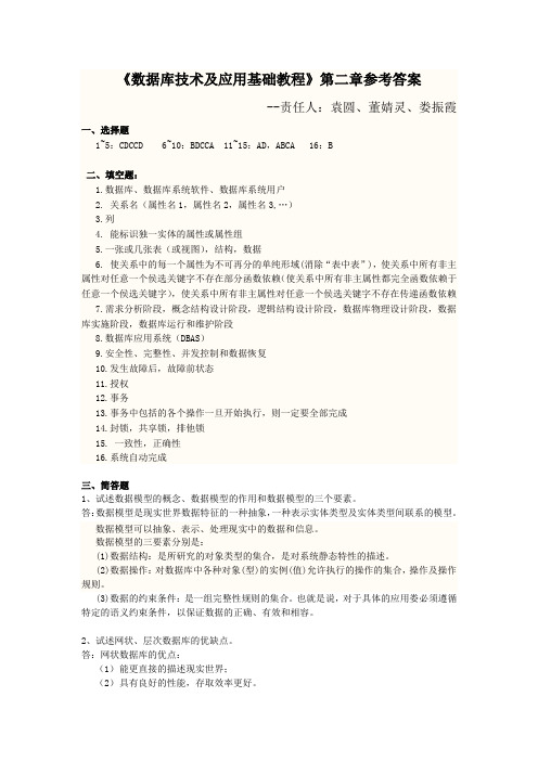
《数据库技术及应用基础教程》第二章参考答案--责任人:袁圆、董婧灵、娄振霞一、选择题1~5:CDCCD 6~10:BDCCA 11~15:AD,ABCA 16:B二、填空题:1.数据库、数据库系统软件、数据库系统用户2. 关系名(属性名1,属性名2,属性名3,…)3.列4. 能标识独一实体的属性或属性组5.一张或几张表(或视图),结构,数据6. 使关系中的每一个属性为不可再分的单纯形域(消除“表中表”),使关系中所有非主属性对任意一个侯选关键字不存在部分函数依赖(使关系中所有非主属性都完全函数依赖于任意一个侯选关键字),使关系中所有非主属性对任意一个侯选关键字不存在传递函数依赖7.需求分析阶段,概念结构设计阶段,逻辑结构设计阶段,数据库物理设计阶段,数据库实施阶段,数据库运行和维护阶段8.数据库应用系统(DBAS)9.安全性、完整性、并发控制和数据恢复10.发生故障后,故障前状态11.授权12.事务13.事务中包括的各个操作一旦开始执行,则一定要全部完成14.封锁,共享锁,排他锁15. 一致性,正确性16.系统自动完成三、简答题1、试述数据模型的概念、数据模型的作用和数据模型的三个要素。
答:数据模型是现实世界数据特征的一种抽象,一种表示实体类型及实体类型间联系的模型。
数据模型可以抽象、表示、处理现实中的数据和信息。
数据模型的三要素分别是:(1)数据结构:是所研究的对象类型的集合,是对系统静态特性的描述。
(2)数据操作:对数据库中各种对象(型)的实例(值)允许执行的操作的集合,操作及操作规则。
(3)数据的约束条件:是一组完整性规则的集合。
也就是说,对于具体的应用娄必须遵循特定的语义约束条件,以保证数据的正确、有效和相容。
2、试述网状、层次数据库的优缺点。
答:网状数据库的优点:(1)能更直接的描述现实世界;(2)具有良好的性能,存取效率更好。
网状数据库缺点:(1)结构复杂,应用系统越大数据库结构越复杂;(2)用法复杂,用户不易理解。
数据库系统概论第2章关系数据库精品PPT课件
Supervisor
张清政 张清政 刘逸
speciality
信息 信息 信息
postgraduate
李勇 刘晨 王敏
关系SAP的候选码: (postgraduate) 关系SAP的主码: (postgraduate) 关系SAP的主属性: postgraduate 关系SAP的非码属性:Supervisor , speciality
主码:选定的一个 候选码。 主属性:候选码的诸属性。 非主码属性:不包含在任何候选码中的属性。
8
例子1:
关系 S(S#,SN,SD,SA)
关系S的候选码:(S#) , (SN)
关系S的主码:(S#)
关系S的主属性:S#
关系S的非码属性:SD , SA
例子2:
例子3:
全码
关系SC(S#,C#,G)
关系R(P,W,A)
11
p46
2.2.2关系模式 关系模式简记为: R(A1,A2,…,An) 形式化表示为:五元组 R( U, D, dom,F)
关系名 属性集合 域集合 属性向域的 属性间数据的 映象集合 依赖关系集合
例子:选修关系 可简记为:SC(Sno,Cno,G)
形式化表示为:SC ( U, D, dom,F)
第二章 关系数据库
2.1 关系模型概述 2.2 关系数据结构及形式化定义 2.3 关系的完整性 2.4 关系代数 2.5 关系演算
1
2.1 关系模型概述
(1)单一的数据结构——关系
(2)关系操作
关系模型的操作包括:查询和更新
关系操作的特点:一次一集合方式
非关系操作的特点:一次一记录方式
关系代数语言 关系数据语言 关系演算语言
数据库系统概论第二章笔记

数据库系统概论第二章笔记一、关系数据结构及形式化定义。
1. 关系的定义。
- 关系是一个元组的集合。
在关系数据库中,关系以二维表的形式表示。
例如,一个学生关系(表)可能包含学号、姓名、年龄等列,每一行(元组)代表一个学生的信息。
- 关系模式是对关系的描述,包括关系名、组成该关系的属性名集合等。
例如,学生(学号,姓名,年龄)就是一个关系模式。
2. 关系的性质。
- 列是同质的,即每一列中的数据类型相同。
比如学生关系中的年龄列都是数值类型。
- 不同列可出自同一个域,例如学生关系中的性别列和另一个关系中的人员性别列都来自{男,女}这个域。
- 列的顺序无所谓,行的顺序也无所谓。
这意味着在关系中调整列或行的顺序不影响关系的本质。
- 关系中的任意两个元组不能完全相同。
3. 关系的完整性约束。
- 实体完整性。
- 主属性(组成主键的属性)不能为空值(NULL)。
例如在学生关系中,如果学号是主键,那么每个学生的学号必须有确定的值,不能为NULL。
这是为了保证实体的可区分性。
- 参照完整性。
- 设F是基本关系R的一个或一组属性,但不是关系R的码,K是基本关系S的主码。
如果F与K相对应,则称F是R的外码,并称基本关系R为参照关系,基本关系S为被参照关系。
参照关系中的外码值或者为空值,或者是被参照关系中某个元组的主码值。
例如,选课关系(学号,课程号,成绩)中的学号是参照学生关系(学号,姓名,年龄)中学号的外码,选课关系中的学号值必须是学生关系中存在的学号或者为空值(如果允许未注册学生选课的特殊情况)。
- 用户定义完整性。
- 这是针对某一具体应用环境下的关系数据库所制定的约束条件。
例如,学生的年龄可能被限制在一定范围内(如15 - 40岁),成绩可能被限制在0 - 100分之间等。
二、关系代数。
1. 传统的集合运算。
- 并(Union)- 关系R和关系S具有相同的目n(即两个关系都有n个属性),相应的属性取自同一个域。
R∪S是由属于R或属于S的元组组成的集合。
数据库系统教程复习提纲

复习提纲
第2章关系模型和关系运算理论
(1)基本概念
关系模型,关键码(主键和外键),关系的定义和性质,三类完整性规则。
(2)关系代数
五个基本操作,四个组合操作,七个扩充操作。
例2.2~2.13,习题2.6、2.7、2.17
第3章关系数据库语言SQL
(1)SQL数据库的体系结构,SQL的组成。
(2)SQL的数据定义:SQL模式、基本表创建和撤销。
(3)SQL的数据查询;SELECT语句的句法,SELECT语句的三种形式及各种限定,基本表的联接操作。
(4)SQL的数据更新:插入、删除和修改语句。
(5)视图的创建和撤销,对视图更新操作的限制。
补充材料《数据库和数据表管理》中的T-SQL语句
考试中使用T-SQL或者书上语法的都算对,明确要求使用T-SQL语法的除外
例3.1~3.5,3.8~3.19(EXISTS不要求),习题3.2(7、8题不要求),3.7,3.12~3.14
第4章关系数据库的规范化设计
1NF,2NF,3NF判断和分解算法
习题4.26~4.29
第5章数据库设计和ER模型
(1)根据要求写出ER模型
(2)ER模型到关系模型的转换,标出主键及外键
例5.2~5.5,5.9~5.11,5.4节(PPT中有转换结果),习题5.13~5.15,5.19
第七章系统实现技术
以补充PPT为主,掌握对应的T-SQL语句
(1)SQL SERVER对事务的支持
(2)数据备份与恢复
(3)数据完整性(考试可能和第三章内容在一起)
(4)数据库安全性。
数据库系统原理复习.ppt

• 分析上述异常后得出的结论——规范化(实施)
• 函数依赖的定义(熟知) • 平凡的函数依赖、非平凡函数依赖。 (熟知)
2019-8-18
谢谢观赏
22
•完全函数依赖、部分函数依赖。 (熟知)
• 传递函数依赖、直接函数依赖。 (熟知)
• 候选码、主码、主属性、非主属性(非码属性)、全码、外 码。 (熟知)
2019-8-18
谢谢观赏
19
• 视图功能(实施) 视图的概念 视图的定义语句(视图列名定义的3个要求) 单表视图、多表视图、基于视图的视图、表达式视图、集
函数视图。。。 视图的删除 视图的更新:插入、删除、修改。(with check option) 视图的查询
•数据库控制功能(实施) 授权语句 回收权限语句 完整性控制语句 (以及后面讲到的并发、恢复等控制语句)
• 范式的含义(熟知)
• 1NF——2NF——3NF——BCNF——4NF之间的关系及结论。
• 多值依赖的概念、性质、4NF。 (了解)
• 模式的分解
分解的定义(理解)
分解的多样性(理解)
分解的正确性——无损连接性、依赖保持性——“等价”
的三个定义。(熟知)
2019-8-18
谢谢观赏
23
第5章 数据库保护——知识点 安全性控制、完整性控制、并发控制、DB恢复
安全性
•安全性控制的概念(了解) • DBS安全控制的机制(了解) • DBS安全控制的一般方法(了解)
用户鉴别、访问控制(自主、强制)、视图、审计、加 密。 • ORACLE的安全控制机制(了解)
用户鉴别、操作授权、系统权限、访问对象权限(表级、 行级、列级)、角色、审计、用户定义安全性、触发器。
数据库系统教程第2章精选全文

M
上海
S3
XIA
19
F
四川
图2.1 学生登记表
• 在关系模型中,字段称为属性,字段值称为属性值,记录类型 称为关系模式。
• 在图2.2中,关系模式名是R。 • 记 录 称 为 元 组 (tuple) , 元 组 的 集 合 称 为 关 系 (relation) 或 实 例
(instance)。 • 一般用大写字母A、B、C、… 表示单个属性,用大写字母 …、
第2章 关系模型和 关系运算理论
本章重要概念
• (1)基本概念
• 关系模型,关键码(主键和外键),关系的定义和性质,三类完 整性规则,过程性语言与非过程性语言。
• (2)关系代数
• 五个基本操作,四个组合操作,七个扩充操作。
• (3)关系代数表达式的优化
• 关系代数表达式的等价及等价转换规则,启化式优化算法。
2.1.1 基本术语
• 定义2.1 用二维表格表示实体集,用关键码进行数据导航的数据模 型称为关系模型(Relational Model)。这里数据导航(data navigation)
是指从已知数据查找未知数据的过程和方法。
学号
姓名
年龄
性别
籍贯
S1
WANG
20
M
北京
S4
LIU
18
F
山东
S2
HU
17
X、Y、Z表示属性集,用小写字母表示属性值,有时也习惯称呼 关系为表或表格,元组为行(row),属性为列(column)。 • 关 系 中 属 性 个 数 称 为 “ 元 数 ” (arity) , 元 组 个 数 为 “ 基 数”(cardinality)。
• 关系元数为5,基数为4
- 1、下载文档前请自行甄别文档内容的完整性,平台不提供额外的编辑、内容补充、找答案等附加服务。
- 2、"仅部分预览"的文档,不可在线预览部分如存在完整性等问题,可反馈申请退款(可完整预览的文档不适用该条件!)。
- 3、如文档侵犯您的权益,请联系客服反馈,我们会尽快为您处理(人工客服工作时间:9:00-18:30)。
Exercise 2.2.1aFor relation Accounts, the attributes are:acctNo, type, balanceFor relation Customers, the attributes are:firstName, lastName, idNo, accountExercise 2.2.1bFor relation Accounts, the tuples are:(12345, savings, 12000),(23456, checking, 1000),(34567, savings, 25)For relation Customers, the tuples are:(Robbie, Banks, 901-222, 12345),(Lena, Hand, 805-333, 12345),(Lena, Hand, 805-333, 23456)Exercise 2.2.1cFor relation Accounts and the first tuple, the components are: 123456 → acctNosavings → type12000 → balanceFor relation Customers and the first tuple, the components are: Robbie → firstNameBanks → lastName901-222 → idNo12345 → accountExercise 2.2.1dFor relation Accounts, a relation schema is:Accounts(acctNo, type, balance)For relation Customers, a relation schema is:Customers(firstName, lastName, idNo, account) Exercise 2.2.1eAn example database schema is:Accounts (acctNo,type,balance)Customers (firstName,lastName,idNo,account)Exercise 2.2.1fA suitable domain for each attribute:acctNo → Integertype → Stringbalance → IntegerfirstName → StringlastName → StringidNo → String (because there is a hyphen we cannot use Integer)account → IntegerExercise 2.2.1gAnother equivalent way to present the Account relation:Another equivalent way to present the Customers relation:Exercise 2.2.2Examples of attributes that are created for primarily serving as keys in a relation:Universal Product Code (UPC) used widely in United States and Canada to track products in stores.Serial Numbers on a wide variety of products to allow the manufacturer to individually track each product.Vehicle Identification Numbers (VIN), a unique serial number used by the automotive industry to identify vehicles.Exercise 2.2.3aWe can order the three tuples in any of 3! = 6 ways. Also, the columns can be ordered in any of 3! = 6 ways. Thus, the number of presentations is 6*6 = 36. Exercise 2.2.3bWe can order the three tuples in any of 5! = 120 ways. Also, the columns can be ordered in any of 4! = 24 ways. Thus, the number of presentations is120*24 = 2880Exercise 2.2.3cWe can order the three tuples in any of m! ways. Also, the columns can be ordered in any of n! ways. Thus, the number of presentations is n!m!Exercise 2.3.1aCREATE TABLE Product (maker CHAR(30),model CHAR(10) PRIMARY KEY,type CHAR(15));Exercise 2.3.1bCREATE TABLE PC (model CHAR(30),speed DECIMAL(4,2),ram INTEGER,hd INTEGER,price DECIMAL(7,2));Exercise 2.3.1cCREATE TABLE Laptop (model CHAR(30),speed DECIMAL(4,2),ram INTEGER,hd INTEGER,screen DECIMAL(3,1),price DECIMAL(7,2));Exercise 2.3.1dCREATE TABLE Printer (model CHAR(30),color BOOLEAN,type CHAR (10),price DECIMAL(7,2));Exercise 2.3.1eALTER TABLE Printer DROP color;Exercise 2.3.1fALTER TABLE Laptop ADD od CHAR (10) DEFAULT ‘none’; Exercise 2.3.2aCREATE TABLE Classes (class CHAR(20),type CHAR(5),country CHAR(20),numGuns INTEGER,bore DECIMAL(3,1),displacement INTEGER);Exercise 2.3.2bCREATE TABLE Ships (name CHAR(30),class CHAR(20),launched INTEGER);Exercise 2.3.2cCREATE TABLE Battles (name CHAR(30),date DATE);Exercise 2.3.2dCREATE TABLE Outcomes (ship CHAR(30),battle CHAR(30),result CHAR(10));Exercise 2.3.2eALTER TABLE Classes DROP bore;Exercise 2.3.2fALTER TABLE Ships ADD yard CHAR(30);Exercise 2.4.1aR1 := σspeed ≥ 3.00 (PC)R2 := πmodel(R1)model100510061013Exercise 2.4.1bR1 := σhd ≥ 100 (Laptop)R2 := Product (R1)R3 := πmaker (R2)makerEABFGExercise 2.4.1cR1 := σmaker=B (Product PC)R2 := σmaker=B (Product Laptop)R3 := σmaker=B (Product Printer)R4 := πmodel,price (R1)R5 := πmodel,price (R2)R6: = πmodel,price (R3)R7 := R4 R5 R6model price1004 6491005 6301006 10492007 1429Exercise 2.4.1dR1 := σcolor = true AND type = laser (Printer)R2 := πmodel (R1)model30033007Exercise 2.4.1eR1 := σtype=laptop (Product)R2 := σtype=PC(Product)R3 := πmaker(R1)R4 := πmaker(R2)R5 := R3 – R4makerFGExercise 2.4.1fR1 := ρPC1(PC)R2 := ρPC2(PC)R3 := R1 (PC1.hd = PC2.hd AND PC1.model <> PC2.model) R2R4 := πhd(R3)hd25080160Exercise 2.4.1gR1 := ρPC1(PC)R2 := ρPC2(PC)R3 := R1 (PC1.speed = PC2.speed AND PC1.ram = PC2.ram AND PC1.model < PC2.model) R2R4 := πPC1.model,PC2.model(R3)PC1.model PC2.model1004 1012Exercise 2.4.1hR1 := πmodel(σspeed ≥ 2.80(PC)) πmodel(σspeed ≥ 2.80(Laptop))R2 := πmaker,model(R1 Product)R3 := ρR3(maker2,model2)(R2)R4 := R2 (maker = maker2 AND model <> model2) R3R5 := πmaker(R4)makerBEExercise 2.4.1iR1 := πmodel,speed(PC)R2 := πmodel,speed(Laptop)R3 := R1 R2R4 := ρR4(model2,speed2)(R3)R5 := πmodel,speed (R3 (speed < speed2 ) R4)R6 := R3 – R5R7 := πmaker(R6 Product)makerBExercise 2.4.1jR1 := πmaker,speed(Product PC)R2 := ρR2(maker2,speed2)(R1)R3 := ρR3(maker3,speed3)(R1)R4 := R1 (maker = maker2 AND speed <> speed2) R2R5 := R4 (maker3 = maker AND speed3 <> speed2 AND speed3 <> speed) R3R6 := πmaker(R5)makerADEExercise 2.4.1kR1 := πmaker,model(Product PC)R2 := ρR2(maker2,model2)(R1)R3 := ρR3(maker3,model3)(R1)R4 := ρR4(maker4,model4)(R1)R5 := R1 (maker = maker2 AND model <> model2) R2R6 := R3 (maker3 = maker AND model3 <> model2 AND model3 <> model) R5R7 := R4 (maker4 = maker AND (model4=model OR model4=model2 OR model4=model3)) R6R8 := πmaker(R7)makerABDEExercise 2.4.2aπmodelσspeed≥3.00PCExercise 2.4.2bLaptopσhd ≥ 100 ProductmakerExercise 2.4.2cσmaker=B πmodel,price σmaker=B πmodel,price σmaker=B πmodel,priceProduct PC Laptop Printer ProductProductExercise 2.4.2d Printerσcolor = true AND type = laserπmodelExercise 2.4.2eσtype=laptopσtype=PC πmakerπmaker ProductProductExercise 2.4.2fρPC1ρPC2 (PC1.hd = PC2.hd AND PC1.model <> PC2.model)πhdPC PCExercise 2.4.2gρPC1ρPC2PC PC(PC1.speed = PC2.speed AND PC1.ram = PC2.ram AND PC1.model < PC2.model)πPC1.model,PC2.modelExercise 2.4.2hPC Laptopσspeed ≥ 2.80σspeed ≥ 2.80πmodelπmodel πmaker,modelρR3(maker2,model2)(maker = maker2 AND model <> model2)makerExercise 2.4.2iPC LaptopProductπmodel,speed πmodel,speed ρR4(model2,speed2)πmodel,speed(speed < speed2 )–makerExercise 2.4.2jProduct PC πmaker,speed ρR3(maker3,speed3)ρR2(maker2,speed2)(maker = maker2 AND speed <> speed2)(maker3 = maker AND speed3 <> speed2 AND speed3 <> speed)makerExercise 2.4.2kπmaker(maker4 = maker AND (model4=model OR model4=model2 OR model4=model3)) (maker3 = maker AND model3 <> model2 AND model3 <> model)(maker = maker2 AND model <> model2)ρR2(maker2,model2)ρR3(maker3,model3)ρR4(maker4,model4)πmaker,modelProduct PCExercise 2.4.3aR1 := σbore ≥ 16 (Classes)R2 := πclass,country (R1)Exercise 2.4.3bR1 := σlaunched < 1921 (Ships)R2 := πname (R1)RamilliesRenownRepulseResolutionRevengeRoyal OakRoyal SovereignTennesseeExercise 2.4.3cR1 := σbattle=Denmark Strait AND result=sunk(Outcomes)R2 := πship (R1)shipBismarckHoodExercise 2.4.3dR1 := Classes ShipsR2 := σlaunched > 1921 AND displacement > 35000 (R1)R3 := πname (R2)nameIowaMissouriMusashiNew JerseyNorth CarolinaWashingtonWisconsinYamatoExercise 2.4.3eR1 := σbattle=Guadalcanal(Outcomes)R2 := Ships (ship=name) R1R3 := Classes R2R4 := πname,displacement,numGuns(R3)name displacement numGuns Kirishima 32000 8Washington 37000 9Exercise 2.4.3fR1 := πname(Ships)R2 := πship(Outcomes)R3 := ρR3(name)(R2)R4 := R1 R3nameCaliforniaHarunaHieiIowaKirishimaKongoMissouriMusashiNew JerseyNorth CarolinaRamilliesRenownRepulseResolutionRevengeRoyal OakRoyal SovereignTennesseeWashingtonExercise 2.4.3gFrom 2.3.2, assuming that every class has one ship named after the class. R1 := πclass (Classes)R2 := πclass (σname <> class (Ships))R3 := R1 – R2Exercise 2.4.3hR1 := πcountry (σtype=bb (Classes))R2 := πcountry (σtype=bc (Classes))R3 := R1 ∩ R2Exercise 2.4.3iR1 := πship,result,date (Battles (battle=name) Outcomes)R2 := ρR2(ship2,result2,date2)(R1)R3 := R1 (ship=ship2 AND result=damaged AND date < date2) R2R4 := πship (R3)No results from sample data.Exercise 2.4.4aσbore ≥ 16πclass,country ClassesExercise 2.4.4bσlaunched < 1921πname ShipsExercise 2.4.4cWisconsin Yamato Arizona Bismarck Duke of York Fuso Hood King George V Prince of WalesRodneyScharnhorstSouth Dakota West VirginiaYamashiro classBismarckcountryJapanGt. BritainOutcomesπshipσbattle=Denmark Strait AND result=sunkExercise 2.4.4dClasses Shipsσlaunched > 1921 AND displacement > 35000πnameExercise 2.4.4eσbattle=Guadalcanal Outcomes Classes(ship=name)πname,displacement,numGunsExercise 2.4.4fShipsOutcomesπnameπship ρR3(name)Exercise 2.4.4g ClassesShips πclass σname <> class πclass –Exercise 2.4.4hClasses Classes σtype=bb σtype=bcπcountry πcountry∩Exercise 2.4.4iπship(ship=ship2 AND result=damaged AND date < date2)ρR2(ship2,result2,date2)πship,result,date(battle=name)Battles OutcomesExercise 2.4.5The result of the natural join has only one attribute from each pair of equated attributes. On the other hand, the result of the theta-join has both columns of the attributes and their values are identical.Exercise 2.4.6UnionIf we add a tuple to the arguments of the union operator, we will get all of the tuples of the original result and maybe the added tuple. If theadded tuple is a duplicate tuple, then the set behavior will eliminate that tuple. Thus the union operator is monotone.IntersectionIf we add a tuple to the arguments of the intersection operator, we will get all of the tuples of the original result and maybe the added tuple. If the added tuple does not exist in the relation that it is added but does exist in the other relation, then the result set will include the added tuple.Thus the intersection operator is monotone.DifferenceIf we add a tuple to the arguments of the difference operator, we may not get all of the tuples of the original result. Suppose we have relations R and S and we are computing R – S. Suppose also that tuple t is in R but not in S. The result of R – S would include tuple t. However, if we add tuple t to S, then the new result will not have tuple t. Thus the difference operator is not monotone.ProjectionIf we add a tuple to the arguments of the projection operator, we will get all of the tuples of the original result and the projection of the added tuple. The projection operator only selects columns from the relation and does not affect the rows that are selected. Thus the projection operator is monotone.SelectionIf we add a tuple to the arguments of the selection operator, we will get all of the tuples of the original result and maybe the added tuple. If the added tuple satisfies the select condition, then it will be added to the new result. The original tuples are included in the new result because they still satisfy the select condition. Thus the selection operator is monotone.Cartesian ProductIf we add a tuple to the arguments of the Cartesian product operator, we will get all of the tuples of the original result and possibly additional tuples. The Cartesian product pairs the tuples of one relation with the tuples of another relation. Suppose that we are calculating R x S where R has m tuples and S has n tuples. If we add a tuple to R that is not already in R, then we expect the result of R x S to have (m + 1) * n tuples.Thus the Cartesian product operator is monotone.Natural JoinsIf we add a tuple to the arguments of a natural join operator, we will get all of the tuples of the original result and possibly additional tuples.The new tuple can only create additional successful joins, not less. If, however, the added tuple cannot successfully join with any of theexisting tuples, then we will have zero additional successful joins. Thus the natural join operator is monotone.Theta JoinsIf we add a tuple to the arguments of a theta join operator, we will get all of the tuples of the original result and possibly additional tuples. The theta join can be modeled by a Cartesian product followed by a selection on some condition. The new tuple can only create additional tuples in the result, not less. If, however, the added tuple does not satisfy the select condition, then no additional tuples will be added to the result. Thus the theta join operator is monotone.RenamingIf we add a tuple to the arguments of a renaming operator, we will get all of the tuples of the original result and the added tuple. The renaming operator does not have any effect on whether a tuple is selected or not. In fact, the renaming operator will always return as many tuples as its argument. Thus the renaming operator is monotone.Exercise 2.4.7aIf all the tuples of R and S are different, then the union has n + m tuples, and this number is the maximum possible.The minimum number of tuples that can appear in the result occurs if every tuple of one relation also appears in the other. Then the union has max(m , n) tuples.Exercise 2.4.7bIf all the tuples in one relation can pair successfully with all the tuples in the other relation, then the natural join has n * m tuples. This number would be the maximum possible.The minimum number of tuples that can appear in the result occurs if none of the tuples of one relation can pair successfully with all the tuples in the other relation. Then the natural join has zero tuples.Exercise 2.4.7cIf the condition C brings back all the tuples of R, then the cross product will contain n * m tuples. This number would be the maximum possible.The minimum number of tuples that can appear in the result occurs if the condition C brings back none of the tuples of R. Then the cross product has zero tuples.Exercise 2.4.7dAssuming that the list of attributes L makes the resulting relation πL(R) and relation S schema compatible, then the maximum possible tuples is n. This happens when all of the tuples of πL(R) are not in S.The minimum number of tuples that can appear in the result occurs when all of the tuples in πL(R) appear in S. Then the difference has max(n–m , 0) tuples.Exercise 2.4.8Defining r as the schema of R and s as the schema of S:1.πr(R S)2.R δ(πr∩s(S)) where δ is the duplicate-elimination operator in Section 5.2 pg. 2133.R – (R –πr(R S))Exercise 2.4.9Defining r as the schema of R1.R - πr(R S)Exercise 2.4.10πA1,A2…An(R S)Exercise 2.5.1aσspeed < 2.00 AND price > 500(PC) = øModel 1011 violates this constraint.Exercise 2.5.1bσscreen < 15.4 AND hd < 100 AND price ≥ 1000(Laptop) = øModel 2004 violates the constraint.Exercise 2.5.1cπmaker(σtype = laptop(Product)) ∩ πmaker(σtype = pc(Product)) = øManufacturers A,B,E violate the constraint.Exercise 2.5.1dThis complex expression is best seen as a sequence of steps in which we define temporary relations R1 through R4 that stand for nodes of expression trees. Here is the sequence:R1(maker, model, speed) := πmaker,model,speed(Product PC)R2(maker, speed) := πmaker,speed(Product Laptop)R3(model) := πmodel(R1 R1.maker = R2.maker AND R1.speed ≤ R2.speed R2)R4(model) := πmodel(PC)The constraint is R4 ⊆ R3Manufacturers B,C,D violate the constraint.Exercise 2.5.1eπmodel(σLaptop.ram > PC.ram AND Laptop.price ≤ PC.price(PC × Laptop)) = øModels 2002,2006,2008 violate the constraint.Exercise 2.5.2aπclass(σbore > 16(Classes)) = øThe Yamato class violates the constraint.Exercise 2.5.2bπclass(σnumGuns > 9 AND bore > 14(Classes)) = øNo violations to the constraint.Exercise 2.5.2cThis complex expression is best seen as a sequence of steps in which we define temporary relations R1 through R5 that stand for nodes of expression trees. Here is the sequence:R1(class,name) := πclass,name(Classes Ships)R2(class2,name2) := ρR2(class2,name2)(R1)R3(class3,name3) := ρR3(class3,name3)(R1)R4(class,name,class2,name2) := R1 (class = class2 AND name <> name2) R2R5(class,name,class2,name2,class3,name3) := R4 (class=class3 AND name <> name3 AND name2 <> name3) R3The constraint is R5 = øThe Kongo, Iowa and Revenge classes violate the constraint.Exercise 2.5.2dπcountry(σtype = bb(Classes)) ∩ πcountry(σtype = bc(Classes)) = øJapan and Gt. Britain violate the constraint.Exercise 2.5.2eThis complex expression is best seen as a sequence of steps in which we define temporary relations R1 through R5 that stand for nodes of expression trees. Here is the sequence:R1(ship,battle,result,class) := πship,battle,result,class(Outcomes (ship = name) Ships)R2(ship,battle,result,numGuns) := πship,battle,result,numGuns(R1 Classes)R3(ship,battle) := πship,battle(σnumGuns < 9 AND result = sunk (R2))R4(ship2,battle2) := ρR4(ship2,battle2)(πship,battle(σnumGuns > 9(R2)))R5(ship2) := πship2(R3 (battle = battle2) R4)The constraint is R5 = øNo violations to the constraint. Since there are some ships in the Outcomes table that are not in the Ships table, we are unable to determine the number of guns on that ship.Exercise 2.5.3Defining r as the schema A1,A2,…,A n and s as the schema B1,B2,…,B n:πr(R) πs(S) = øwhere is the antisemijoinExercise 2.5.4The form of a constraint as E1 = E2 can be expressed as the other two constraints.Using the “equating an expression to the empty set” method, we can simply say:E1– E2 = øAs a containment, we can simply say:E1⊆ E2 AND E2⊆ E1Thus, the form E1 = E2 of a constraint cannot express more than the two other forms discussed in this section.。