Fluent二维波浪模拟教程
Fluent模拟的基本步骤
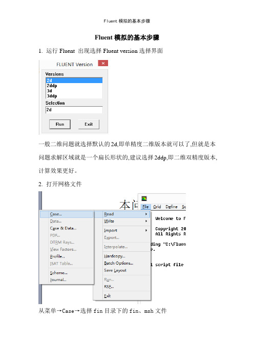
Fluent模拟的基本步骤1.运行Fluent 出现选择Fluent version选择界面一般二维问题就选择默认的2d,即单精度二维版本就可以了,但就是本问题求解区域就是一个扁长形状的,建议选择2ddp,即二维双精度版本,计算效果更好。
2.打开网格文件从菜单→Case→选择fin目录下的fin、msh文件3.指定计算区域的实际尺寸在Gambit建立区域时没有尺寸的单位,此时应该进行确定,也可以对区域进行放大或缩小等。
在菜单Grid下选择Scale出现上面的对话框。
将其中的Grid wascreated by 中的单位m,更改为mm,此时scale factor X与Y都出现0、001。
然后按Scale4.选择模型该问题就是稳态问题,在Solver 中已经就是默认,只就是求解温度场。
由菜单Define →Models→Energy然后选择Energy Equation。
5.指定边界条件与求解区域的材料需要将求解区域的四个边界进行说明,由菜单单Define →Models →Boundary conditions。
首先设置左边界,即肋根的条件。
点击left项,Type 列表中缺省指定在Wall,所以不需要改变,再点击Set选择thermal conditions列表中的Temperature,并且在右侧Temperature(k)中填入323(即50℃),然后点击OK完成。
按照同样方法对up、down与right 三个边界进行设置。
这三个边界均为对流边界,需要给出表面传热系数与流体温度。
本问题的求解区域为固体,并且设定其物性参数。
在zone 列表中选择zone(在Gambit 中指定的名字),已经就是默认的solid、点击set点击Edit编辑材料的物性,本问题只就是设计材料的导热系数,所以仅需将导热系数的值更改为160,然后点击Change后再close,上一个页面后按ok。
此时可关闭Boundary conditions。
fluent二维大涡模拟命令
fluent二维大涡模拟命令Fluent是流体动力学模拟软件的一种,它提供了二维大涡模拟命令用于模拟二维涡旋动力学过程。
本文将分步骤阐述如何使用Fluent二维大涡模拟命令。
第一步,打开Fluent软件。
进入“File”菜单,选择“New”打开一个新的工作文件。
在Fluent主界面的左侧面板选择“2D”选项卡,然后选择“Viscous”和“Steady”选项后点击“Create/Edit”按钮。
第二步,进入“Grid”界面。
在“Mesh”选项卡中选择“2D Mesh”菜单,选择“Triangle”网格类型。
随后,选择“Mechanical”类型并调整所需参数,包括网格的大小、分辨率、以及其他关键点的划分数量。
最后,点击“Generate Mesh”按钮生成网格。
第三步,设置边界条件。
在Fluent主界面的左侧面板选择“Boundary Conditions”选项卡。
根据需要设置边界条件,包括入口和出口边界、容器壁边界和物体边界。
基本的物理条件包括质量流速、温度和密度。
第四步,设置模拟参数。
在Fluent主界面的左侧面板选择“Solution”选项卡。
首先选择“Viscous”和“Steady”选项,然后在“Methods”菜单中选择“Unsteady”. 调整所需参数并计算时间,包括时间步长和计算时间范围。
第五步,开始求解二维大涡模拟。
在Fluent主界面的左侧面板选择“Compute”选项卡,点击“Start Calculation”按钮开始求解。
第六步,查看二维大涡模拟结果。
在Fluent主界面的左侧面板选择“Graphics”选项卡。
根据需要选择显示不同的结果,包括速度分布、温度变化、实体形态等等。
以上是使用Fluent二维大涡模拟命令的步骤。
通过学习和实践,我们可以使用Fluent来分析和解决各种相关的物理、化学和工程问题。
基于Fluent的波浪对海岸冲击的数值模拟
第35卷第4期2020年08月中国海洋平台CHINA OFFSHORE PLATFORMVol.35No.4Aug.,2020文章编号:1001-4500(2020)04-0056-04基于Fluent的波浪对海岸冲击的数值模拟陈从磊1,刘桢S王玉红彳,梁旭$(1•中国石油化工股份有限公司石油勘探开发研究院,北京100083;2•浙江大学海洋学院,浙江舟山316021)摘要:在Fluent软件的基础上,通过流体体积算法,数值模拟波高为0.2m.周期为1.5s、波长为3.5m的波浪对墙体的冲击过程,重点研究波浪对墙体的冲击力作用和网格尺寸对流场变化的影响。
由模拟结果得出:墙体受到的冲击压力在时间历程上具有一定的周期性,但冲击压力的峰值具有一定的随机性;网格尺寸不同会导致自由面重构的不同,从而使流体体积法捕捉到的流场速度和压力不同,网格越精细,捕捉到的冲击压力更精确。
关键词:Fluent软件;海岸冲击;流场;数值模拟中图分类号:U656.2文献标志码:ANumerical Simulation for Impact of Waves on Coast Based on FluentCHEN Conglei1,LIU Zhen2,WANG Yuhong2,LIANG Xu2(1.Institute of Petroleum Exploration and Development,China Petroleumand Chemical Corporation,Beijing100083,China;2.Ocean College,Zhejiang University,Zhoushan316021,Zhejiang,China)Abstract:On the basis of Fluent software,Volume of Fluid(VOF)algorithm is used to numerically simulate the impact of waves on the wall under certain conditions that wave height is0.2m,wave period is1.5s and wave length is3.5m.Main attention is paid to the impact pressure,velocity field and the effects of grid size on the characteristics of the flow field.The simulation results show that:the impact pressure on the wall is of some periodicity in time history but the peak of the impact pressure is of some randomness;different grid sizes will affect different reconstructions of the free surface,so that the speed and pressure of the flow field captured by the VOF method are different,and the finer the grid,the more accurate the captured impact pressure is.Key words:Fluent software;impact on coast;velocity field;numerical simulation0引言我国每年都遭受严重的台风灾害。
fluent的一个实例(波浪管道的内部流动模拟).
基于FLUENT 的波浪管道热传递耦合模拟CFD 可以对热传递耦合的流体流动进行模拟。
CFD 模拟可以观察到管道内部的流动行为和热传递,这样可以改进波浪壁面复杂通道几何形状中的热传递。
目的:(1) 创建由足够数量的完整波浪组成的波浪管道,提供充分发展条件; (2) 应用周期性边界条件创建波浪通道的一部分; (3) 研究不同湍流模型以及壁面函数对求解的影响; (4) 采用固定表面温度以及固定表面热流量条件,确定雷诺数与热特性之间的关系。
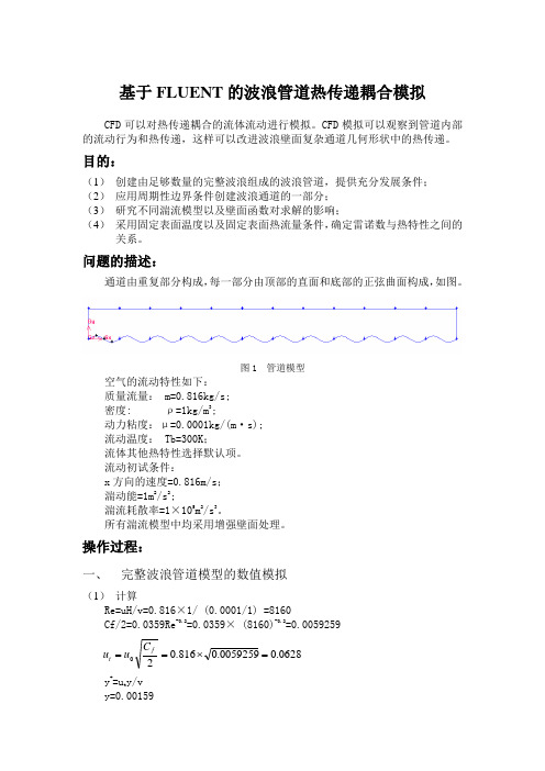
问题的描述:通道由重复部分构成,每一部分由顶部的直面和底部的正弦曲面构成,如图。
图1 管道模型空气的流动特性如下: 质量流量: m=0.816kg/s; 密度: ρ=1kg/m 3;动力粘度:μ=0.0001kg/(m ·s); 流动温度: Tb=300K ;流体其他热特性选择默认项。
流动初试条件:x 方向的速度=0.816m/s ; 湍动能=1m 2/s 2;湍流耗散率=1×10⁵m 2/s 3。
所有湍流模型中均采用增强壁面处理。
操作过程:一、 完整波浪管道模型的数值模拟(1) 计算Re=u H/v=0.816×1/ (0.0001/1) =8160Cf/2=0.0359Re -0.2=0.0359× (8160)-0.2=0.00592590628.00059259.0816.02=⨯==f t C u uy +=u t y/v y=0.00159(2)创建网格本例为波浪形管道,管道壁面为我们所感兴趣的地方所以要局部细化。
入口和出口处的边界网格设置如图。
图2 边网格生成面网格图3 管道网格(3)运用Fluent进行计算本例涉及热传递耦合,所以在fluent中启动能量方程,如图。
图4 能量方程设定条件,湍流模型选择标准k-e模型,近壁面处理选择增强壁面处理。
图5 湍流模型设定材料,密度为1,动力粘度改为0.0001如图。
图6 材料设定设定边界条件,入口速度为0.816,湍动能为1,湍流耗散率为100000。
fluent模拟基本步骤及注意事项
二维模拟:一、模拟类型:1、 大区域空间速度场模拟计算区域大小设置:迎风面是建筑长度的3倍,背风面是建筑长度的12倍,两侧面是建筑宽度的3倍,高度是建筑高度的4倍。
根据相似理论:l C -几何比例尺 速度比例尺:210l C C =υ 风量比例尺:2520l l Q C C C C =⋅=υ 热量比例尺:250l T Q C C C Cq =⋅=∆2、 建筑户型温度场、速度场模拟二、基本操作步骤及注意事项:A gambit 建模1、 建模:方法一:直接在GAMBIT 建模;方法二:CAD 导入gambit ;1) 在CAD 中用PL 线将户型的基本构造画出来,创建为面域;2) 输入命令acisoutver ,把‘70’修改为‘30’。
3) “文件”——“输出”——sat 文件4) 在gambit 中导入Acis 文件注意:在用PL 线构画户型时,在进口和出口边界(窗户、内户门),要各边界端点连续画线。
2、 划分网格:Interval Size :503、 设置边界条件内部开口边界(门)设置为internal ,房间相邻墙壁设置为Wall4、 保存文件,并输出mesh 文件B 导入fluent 计算:1、 导入mesh 文件2、 检查网格3、 设置单位gambit 里可以缩小建筑比例建模,在fluent 中设置单位恢复原模型。
4、 选择计算模型5、 设置材料类型6、 设置边界条件7、 设置模拟控制条件8、 边界初始化9、设置监视窗口10、设置迭代次数进行计算11、结果显示12、保存文件三、需解决问题:1、湍流强度等计算;2、层流湍流界定问题;3、壁面湿度设置问题;四、待提高部分:1、户型流场模拟时,墙壁考虑采用双钱;2、南京理工校区原始模型(不简化)模拟;3、三维模型模拟;五、。
fluent 二维大涡模拟命令
fluent 二维大涡模拟命令Fluent(通常称为ANSYS Fluent)是一种基于计算流体动力学(CFD)的软件,它使用数值方法解决流体力学和热力学方程。
Fluent支持多个求解器,包括稳态、非稳态、可压缩和不可压缩流体求解器。
其中,二维大涡模拟(Large Eddy Simulation,LES)是一种用于模拟湍流流动的CFD方法,通过分解流体的速度场为大尺度和小尺度来模拟湍流流动。
本文将介绍Fluent中二维大涡模拟的相关命令。
1. 设定模拟参数在开始二维大涡模拟前,需要设定一些模拟参数,包括流体属性和边界条件。
在Fluent中,通过以下命令可以设定流体属性和边界条件:(1)设定流体属性DEFINE > MODELS > VISCOSITY2. 定义二维网格在进行CFD模拟前,需要先定义计算网格,以便数值求解器能够在其上执行算法。
在Fluent中,通过以下命令定义二维网格:(1)导入二维网格FILE > IMPORT > MESH3. 指定求解器有关Fluent的求解器已经在第一段中提到。
在进行二维大涡模拟时,可以选择可压缩或不可压缩流体求解器作为替代。
(2)可压缩流体求解器SOLVE > COMPRESSIBLE FLOW/HEAT TRANSFER > STEADY模拟模型是模拟过程中使用的具体模型。
在Fluent中,用户可以选择不同的模拟模型。
(1)可分离流边界层(Detached Eddy Simulation,DES)MODEL > VISCOSITY > DES(2)壁面函数(Wall Function)MODEL > VISCOSITY > WALL FUNCTION在进行CFD模拟时,需要设定一些计算参数以控制模拟进程,以及获得所需的结果。
在Fluent中,用户可以使用以下命令设定计算参数:6. 运行模拟在完成所有设定后,可以通过以下命令在Fluent中运行二维大涡模拟:SOLVE > EXECUTE COMMAND FILE > RUN此时,Fluent将自动执行过程,直至收敛或达到设定的计算时间。
Fluent二维流体动画实例两种方法
二维流体动画实例软件版本Fluent-6.3.26.Gambit-2.2.30.具体步骤1.在Fluen t中导入已经定义好的各种参数条件的cas文件开启Fluen t,选择2ddp,在Fluen t中,“File”—“Read”—“Case&Data”,选择文件夹“Fluent-File”中的“mix-data.cas”文件。
这个二维模型的制作过程在PDF中有说明,上面的文件是已经做好的模型。
2.初始化数据在Fluen t中,“Solve”—“Initia lize”—“Initia lize”,点击“Init”,初始化完后点击“Close”关闭对话框,如图1所示。
图1 初始化数据3.定义动画在Fluen t中,“Solve”—“Animat e”—“Define”,弹出Solu tionAnimati on 对话框,如图2所示的设置。
图2 动画设置对话框接下来点击图2对话框中的“Define”,弹出Anim ation Sequen ce对话框,在“Storag e Type”中选择“PPM Image”,在“Storag e Direct ory”中设置动画序列的保存路径,注意路径不得有中文,在“Displa y Type”中选择“Contou rs”,弹出Cont ours对话框,按自己的显示需要设置好点击或直接点击“Displa y”弹出显示窗口,再点击“Close”完成等值线的设置,想要更改Di splay Type的话则点击“Proper ties”即可,分别如图3~5所示。
图3 动画序列对话框设置图4 显示窗口图5 等值线设置设置完成后,在AnimationSequen ce对话框中点击OK完成设置,再在“Soluti on Animati on”对话框中点击OK完成设置。
基于FLUENT的二维数值波浪水槽研究

基于FLUENT的二维数值波浪水槽研究一、本文概述随着计算流体力学(CFD)技术的快速发展,其在海洋工程、船舶设计、水利水电工程等领域的应用日益广泛。
FLUENT作为一款功能强大的CFD软件,以其灵活的求解器、丰富的物理模型库和强大的后处理功能,受到了广大研究者和工程师的青睐。
数值波浪水槽作为模拟波浪现象的重要工具,对于研究波浪与结构物的相互作用、评估海洋工程结构的稳定性和安全性具有重要意义。
本文旨在利用FLUENT软件建立一个二维数值波浪水槽模型,通过模拟波浪的生成、传播和衰减过程,分析波浪的基本特性。
文章首先介绍了数值波浪水槽的基本原理和FLUENT软件在波浪模拟中的应用,然后详细阐述了二维数值波浪水槽模型的建立过程,包括控制方程的选择、边界条件的设定、网格的生成与优化等。
在此基础上,通过对不同工况下的波浪进行模拟,分析了波浪高度、波长、波速等关键参数的变化规律,并与理论值进行了对比验证。
本文的研究不仅有助于深入理解波浪的传播规律和结构物在波浪作用下的动力响应,还可为相关领域的工程设计和科学研究提供有价值的参考。
通过不断优化数值模型,有望提高波浪模拟的准确性和效率,为推动CFD技术在海洋工程领域的应用提供有力支持。
二、FLUENT软件及其在波浪水槽模拟中的应用FLUENT是一款功能强大的流体动力学仿真软件,广泛应用于各种流体流动、热传导和化学反应等领域的模拟研究。
该软件采用基于有限体积法的数值解法,可以精确地求解流体动力学方程,包括连续性方程、动量方程和能量方程等。
FLUENT还提供了丰富的物理模型库和用户自定义模型的功能,使得用户可以根据实际需求选择合适的模型进行模拟。
在波浪水槽模拟中,FLUENT软件的应用主要体现在以下几个方面:波浪生成与模拟:通过设定特定的边界条件和初始条件,FLUENT 可以模拟出不同波形、波高和周期的波浪。
例如,通过设定造波机的运动规律,可以模拟出规则波或不规则波的生成和传播过程。
- 1、下载文档前请自行甄别文档内容的完整性,平台不提供额外的编辑、内容补充、找答案等附加服务。
- 2、"仅部分预览"的文档,不可在线预览部分如存在完整性等问题,可反馈申请退款(可完整预览的文档不适用该条件!)。
- 3、如文档侵犯您的权益,请联系客服反馈,我们会尽快为您处理(人工客服工作时间:9:00-18:30)。
Tutorial10.Simulation of Wave Generation in a TankIntroductionThe purpose of this tutorial is to illustrate the setup and solution of the2D laminarfluid flow in a tank with oscillating motion of a wall.The oscillating motion of a wall can generate waves in a tank partiallyfilled with a liquid and open to atmosphere.Smooth waves can be generated by setting appropriate frequency and amplitude.One of the tank walls is moved to and fro by specifying a sinusoidal motion.In this tutorial you will learn how to:•Read an existing meshfile in FLUENT.•Check the grid for dimensions and quality.•Add newfluid in the materials list.•Set up a multiphaseflow problem.•Use the dynamic mesh model.•Set up an animation using Execute Commands panel.PrerequisitesThis tutorial assumes that you have little experience with FLUENT but are familiar with the interface.Problem DescriptionIn this tutorial,we consider a rectangular tank with a length(L)of15m and width(W) of0.8m(Figure10.1).The left wall is assigned a motion with sinusoidal time variation.The top wall is open to atmosphere and thus maintained at atmospheric pressure.The flow is assumed to be laminar.Simulation of Wave Generation in a TankFigure10.1:Problem SchematicPreparation1.Copy the meshfile,wave.msh and libudf folder to your working directory.2.Start the2D double precision solver of FLUENT.Setup and SolutionStep1:Grid1.Read the gridfile,wave.msh.File−→Read−→Case...FLUENT will read the meshfile and report the progress in the console window.2.Check the grid.Grid−→CheckThis procedure checks the integrity of the mesh.Make sure the reported minimumvolume is a positive number.3.Check the scale of the grid.Grid−→Scale...Simulation of Wave Generation in a Tank Check the domain extents to see if they correspond to the actual physical dimensions.If not,the grid has to be scaled with proper units.4.Display the grid(Figure10.2).Display−→Grid...(a)Click Colors....The Grid Colors panel opens.i.Under Options,enable Color by ID.ii.Click Close.(b)In the Grid Display panel,click Display(c)Zoom in near the moving-wall(Figure10.3).Simulation of Wave Generation in a TankFigure10.2:Grid DisplayFigure10.3:Grid Display(Close-up of moving-wall)Simulation of Wave Generation in a TankStep2:Models1.Specify the solver settings.Define−→Models−→Solver...(a)Under Time,enable Unsteady(b)Under Transient Controls,enable Non-Iterative Time Advancement.(c)Click OK.2.Enable VOF multiphase model.Define−→Models−→Multiphase...Simulation of Wave Generation in a Tank(a)Under Model,enable Volume of Fluid.The panel expands to show the other settings related to VOF model.Retainthe other settings as default.(b)Click OK.Step3:MaterialsDefine−→Materials...1.Add liquid water to the list offluid materials by copying it from the materialsdatabase.Simulation of Wave Generation in a Tank(a)Click Fluent Database....Fluent Database Materials panel opens.Simulation of Wave Generation in a Tanki.Select water-liquid(h2o<l>)from the Fluent Fluid Materials list.Scroll down to view water-liquid.ii.Click Copy and close the panel.(b)Click Change/Create and close the panel.Step4:PhasesDefine−→Phases...1.Set air as primary phase and water as secondary phase.(a)Under Phase,select phase-1.The Type will be shown as primary-phase.(b)Click Set....i.Change Name to air.ii.Select air in the Phase Material drop-down list.iii.Click OK.(c)Similarly,change the Name of phase-2to water and set its Type to water-liquid.(d)Close the Phases panel.Simulation of Wave Generation in a TankStep5:Operating ConditionsDefine−→Operating Conditions...1.Set the gravitational acceleration.(a)Enable Gravity.(b)Under Gravitational Acceleration,set Y to-9.81m/s2.As the tank bottom is perpendicular to Y axis,gravity points in the negativeY direction.2.Set the operating density.(a)Under Variable-Density Parameters,enable Specified Operating Density.(b)Retain the default density of1.225kg/m3.Set the operating density to the density of the lighter phase.This excludesthe build-up of hydrostatic pressure within the lighter phase,improving theround-offaccuracy for the momentum balance.3.Set the reference pressure location.(a)Under Reference Pressure Location,retain the default value of zero for both Xand Y.This location corresponds to a region where thefluid will always be100%ofone of the phases(water).If it is not,it is recommended to change the regionto a appropriate location where the pressure value does not change much overtime.This condition is essential for smooth and rapid convergence.4.Click OK to accept the settings and close the panel.Simulation of Wave Generation in a TankStep6:Boundary ConditionsFLUENT maintains zero velocity condition on all the walls.Also,the pressure condition for outlet boundary at the top is set by default to zero gauge(or atmospheric).Hence, there is no need to change the boundary conditions.Retain all the boundary conditions as default.Step7:UDF LibraryDefine−→User-Defined−→Functions−→Compiled...1.Click Load to load the UDF library.The sinusoidal wall motion will be assigned using user defined function.A compiledUDF library named libudf is created for this purpose.Step8:Dynamic Mesh Model1.Set the dynamic mesh parameters.Define−→Dynamic Mesh−→Parameters...(a)Under Models,enable Dynamic Mesh.The panel expands.(b)Under Mesh Methods,disable Smoothing and enable Layering.(c)Under the Layering tab,set Collapse Factor to0.4.(d)Click OK.2.Set the dynamic mesh zones.Define−→Dynamic Mesh−→Zones...(a)Under Zone Names,select moving-wall.(b)Under Type,retain the default selection of Rigid Body.(c)Under Meshing Options tab,set Cell Height to0.008m.This is the average size of the cell normal to the moving wall.(d)Click Create and close the panel.Step9:Solution1.Retain the default solution controls.Solve−→Controls−→Solution...Solve−→Initialize−→Initialize...(a)Click Init and close the panel.The complete domain is now initialized with air.The water level required at start(t=0)can be patched.3.Create a register marking the region of initial water level.Adapt−→Region...(a)Set X Max to be15m.(b)Set Y Max to be0.5m.(c)Click Mark and close the panel.FLUENT displays the following message in the console:8510cells marked for refinement,0cells marked for coarsening.4.Patch the initial water level.Solve−→Initialize−→Patch...(a)Under Registers to Patch,select hexahedron-r0.(b)Under Phase,select water.(c)Under Variable,select Volume Fraction.(d)Set Value to1.(e)Click Patch and close the panel.5.Display the zone motion to check the movement of moving-wall.(a)Display the grid(Figure10.4).Display−→Grid...i.Under Surfaces,deselect default-interior.Zoom-in the graphics window to get the view as shown in Figure10.4.ii.Click Display.Figure10.4:Grid Display Outline at t=0(b)Display the zone motion.Display−→Zone Motion...i.Under Motion History Integration,set Time Step to0.001.ii.Set Number of Steps to300.iii.Click Integrate.iv.Under Preview Controls,set Time Step to0.001.v.Set Number of Steps to300.vi.Click Preview to observe the wall motion.vii.Close the Zone Motion panel.6.View the contours of volume fraction for water(Figure10.5).Display−→Contours...(a)Select Phases...and Volume Fraction in the Contours of drop-down lists.(b)Under Phase,select water.(c)Under Options,enable Filled.(d)Click Display and close the panel.Figure10.5:Contours of Volume Fraction for Water7.Enable the plotting of residuals during the calculation.Solve−→Monitors−→Residuals...(a)Under Options,enable Plot.(b)Under Plotting,set Iterations to10.This will display residuals for only the last10iterations.(c)Click OK.8.Set hardcopy settings.File−→Hardcopy...(a)Under Format,select TIFF.(b)Under Coloring,select Color.(c)Click Apply.(d)Click Preview.The background of graphics window is changed to white.FLUENT will displaya question dialog box asking you whether to reset the window.(e)Click Yes in the Question dialog box.(f)Close the panel.9.Set the commands to capture the images of contours.You need to use Text User Interface(TUI)commands to achieve this.For most of the graphical commands,corresponding TUI commands are available.Solve−→Execute Commands...(a)Set the number of Defined Commands to3.(b)Enable On option for all the commands.(c)Under Every,set7for all the commands.(d)Under When,set Time Step for all the commands.(e)For command-1,specify the Command as:display set-window1This command will make the window-1active.(f)For command-2,specify the Command as:display contour water vof01This command will display the contours of water volume fraction in the activewindow.(g)For command-1,specify the Command as:display hard-copy"vof-%t.tif"This command will save the image in the TIF format.The%t option gets replaced with the time step number,when the imagefileis saved.The TIFfiles saved can then be used to create a movie.For theinformation on converting TIFfile to an animationfile,refer to/cfm/graphics01.htm(h)Click OK to accept the settings and close the panel.10.Set the surface monitors.Solve−→Monitors−→Surface...(a)Increase the number of Surface Monitors to1.(b)Enable Plot for monitor-1.(c)Under Every,select Time Step.(d)Click on Define...next to monitor-1.(e)Select Area Weighted Average in the Report Type drop-down list.(f)Select Grid and X-Coordinate in the Report of drop-down list.(g)Under Surfaces,select moving-wall.(h)Click OK to close both the panels.11.Save the case and datafiles(wave-init.cas.gz and wave-init.dat.gz).File−→Write−→Case&Data...Retain the default Write Binary Files option so that you can write a binaryfile.The .gz extension will save zippedfiles on both,Windows and UNIX platforms.12.Start the calculation.Solve−→Iterate...(a)Set the Time Step Size as0.001s(b)Set Number of Time Steps to4000.(c)Click Iterate.Figure10.6:Scaled Residuals13.Save the case and datafiles(wave-4000.cas.gz and wave-4000.dat.gz).Figure10.7:Monitor Plot of Area Weighted Average on moving-wallStep10:Postprocessing1.Displayfilled contours of static pressure(Figure10.8).Display−→Contours...(a)Select Pressure...and Static Pressure in the Contours of drop-down lists.(b)Click Display.The pressure at the bottom of the tank is maximum and goes on decreasingtowards the top.This shows the variation of hydrostatic pressure due to theheight of the liquid.Figure10.8:Contours of Static PressureSummaryThe dynamic mesh model is used to apply periodic sinusoidal motion to the wall.This generates a wave in thefluid.The VOF model is used to track the air-water interface and consequently the wave motion.Non-iterative time advancement(NITA)was used to reduce the run time of transient simulation.Images displaying contours of water phase were captured to visualize the transient effects.References1.Flow Around the Itsukushima Gate,an example from Fluent Inc.Marketing Cata-log,2003.Exercises/Discussions1.Run the simulation for longerflow time to check the wave pattern.2.Try running the simulation without non-iterative time advancement(NITA)option.(a)Are theflow patterns different?(b)Compare the wall clock time taken to reach the sameflow time.3.Run the simulation using variable time step option.4.Try different motions to the wall and observe wave patterns.This will need specific C compiler to create UDF library from the source code.5.What other situation can be simulated using the same meshfile?Links for Further Reading•http://www.prads2004.de/pdf/027.pdf•http://www.prads2004.de/pdf/138.pdf•http://www.math.rug.nl/∼veldman/preprints/OMAE2004-51084.pdf。