[2011-paper]Multicore OS benchmarks--we can do better
2011最新CPU型号规格明细表-ALL(爱尚卓越ISRY)
2010 CPU速查目录一、英特尔酷睿i7处理器 ..........................................................................................................................二、英特尔酷睿 2 至尊处理器 ..................................................................................................................三、英特尔酷睿2 四核处理器.................................................................................................................四、英特尔酷睿2 双核处理器...............................................................................................................五、英特尔酷睿 2 双核低压......................................................................................................................六、英特尔酷睿 2 双核超低压 ..................................................................................................................七、英特尔酷睿双核处理器........................................................................................................................八、英特尔酷睿双核处理器采用低压........................................................................................................九、英特尔酷睿双核处理器采用超低压 .............................................................................................十、英特尔酷睿2 单核处理器英特尔...................................................................................................十一、英特尔酷睿单核处理器 .............................................................................................................十二、英特尔酷睿单核处理器超低压.................................................................................................十三、英特尔奔腾处理器至尊版..........................................................................................................十四、英特尔奔腾 D 处理器................................................................................................................十五、英特尔奔腾处理器 ....................................................................................................................十六、英特尔奔腾 4 处理器.................................................................................................................十七、英特尔奔腾M 处理器 ...............................................................................................................十八、英特尔奔腾M 处理器低压..........................................................................................................十九、英特尔奔腾M 处理器超低压 .........................................................................................................二十、移动式英特尔奔腾4处理器 .............................................................................................................二十一、英特尔赛扬处理器........................................................................................................................二十二、英特尔赛扬D 处理器 ..................................................................................................................二十三、英特尔赛扬处理器........................................................................................................................二十四、超低压英特尔赛扬M 处理器 .......................................................................................................二十五、英特尔赛扬处理器........................................................................................................................二十六、英特尔至强处理器7000 型..........................................................................................................二十七、英特尔至强处理器5000 型..........................................................................................................二十八、英特尔至强处理器3000 型 ..........................................................................................................二十九、英特尔安腾处理器........................................................................................................................三十、AMD Desktop Processor Solutions ......................................................................................................三十一、AMD Opteron™ Processor Solutions ...............................................................................................三十二、AMD Opteron™ Processor Solutions ...............................................................................................三十三、Notebook Processor Solutions .........................................................................................................三十四、AMD64 High-End Embedded Processor Solutions .............................................................................一、英特尔酷睿i7处理器世界上性能最强的台式机处理器。
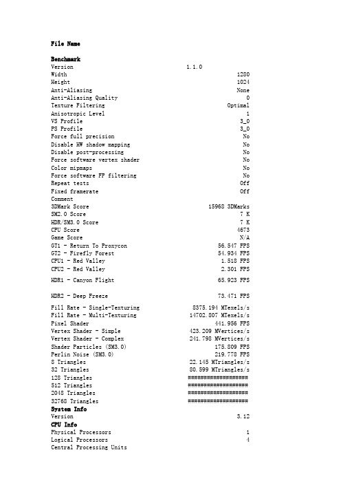
3dmark测试结果
Ext CPUIDs
Intel Intel(R) Xeon(R) CPU W3530 @ 2.80GHz 64-bit
2800 MHz 2800 MHz
0 Hz
8 Processor Cores Available - 0 HTT Processors per Core MMX, CMov, RDTSC, SSE, SSE2, SSE3, PAE, NX Intel(R) Xeon(R) CPU W3530 @ 2.80GHz来自Capabilities
VGA Memory Clock VGA Core Clock Max VGA Memory Clock Max VGA Core Clock DirectShow Info Version Registered DirectShow Filters
16-bit RGB [555] 16-bit ARGB [1555] 16-bit ARGB [4444] 8-bit A [8] 8-bit YUV [800] 16-bit AYUV [8800] FourCC [DXT1] FourCC [DXT2] FourCC [DXT3] FourCC [DXT4] FourCC [DXT5]
16 Kpx 16 Kpx
8 8 8 8 3 3 0 8
NVIDIA Quadro 4000 0x10de 0x06dd 0x078010de 0x00a3
FALSE 0
0x00000000
0x00000000
32-bit ARGB [8888] 32-bit RGB [888] 16-bit RGB [565]
0 Hz 0 Hz 0 Hz 0 Hz
6.6.7600.16385
英特尔推出Parallel Studio XE2011和Cluster Studio2011

O 使 的最小值 ( 菱形部分 ) 因此 由 T , X所送出的测试信 试 ,并 且 研 发 出多颗 S C芯 片 同步 测 试 的技 术 ,
得客户的量产测试成本可以持续 的下降。尽管测试
的成本 下 降 , 所提 供 的测试 质 量并 没有 因此 下降 , 但 客 户 所 收 到 的 S C芯 片仍 会 是 经 过 完 整 测试 的 高 O
成的影响。唯高速信号专用 P B板材价格高昂 , C 且
除 了 P B板 材外 , 有许 多 测试 载板 设 计 的 因素 会 C 还 导 致高 速信 号在 载板 上发 生衰 减 ,或是 让 高速信 号 受 到 噪声 的干扰 。
图 2测试载板上的 ST AA信 号仿 真 眼 图
智原科技的测试工程团队拥有丰富的高速信号
作者简 介
5 结 论 与展 望
高速设 备 的信号 传输 速度 不 断 的提升 ,使 得单 位 时问 内可被 传输 的数 据量倍 数 的增 加 。然 而测试 这 些 内 含高 速 I P的 S C芯 片 的 困难 度 也持 续 地 提 O 高 。高速 I P内建 自测试 技 术让 高 速 I P的量 产测 试
【】 集 成 电 路 l国
C hi na n eg r e d C icui It at r 生衰 减或 是受 到 噪声
的影 响 ,就 可能会 让 内建 自测 试将 原 本性 能正 常 的
芯 片 判 断 为 测 试 不 通 过 。若 选 用 高 速 信 号 专 用 的 P B板 材来 制作 测 试载 板 , 可 以改 善 上述 情 况 造 C 则
陈宏 铭 , 术 市场部 总监 智原 科技 ( 海 ) 限公 技 上 有
司。
硬 件成本 不增 加 的前 提下 达成 目标 。
多核测试利器 CINEBENCH

多核测试利器CINEBENCH
Rock
【期刊名称】《电脑迷》
【年(卷),期】2008(000)014
【摘要】多核处理器已经逐渐成为主流,可遗憾的是目前专门针对多核处理器设计的软件还比较少,无法真正展示出多核处理器的性能优势。
Maxon公司出品的CINEBENCH是一款受到业界人士一致好评的基础测试软件,更重要的是它针对多核计算进行了专门设计,能够充分反映出多核处理器的优势所在。
【总页数】1页(P43-43)
【作者】Rock
【作者单位】
【正文语种】中文
【中图分类】TP3
【相关文献】
1.基于测试向量压缩的多核并行测试 [J], 于静;梁华国;蒋翠云
2.Intel C++9.0:迈向多核CPU时代的终极优化利器 [J], 黄甫
3.多核DSP在就地化保护测试中的关键技术研究 [J], 汪冬辉;王志华;陈明;黄志华;裘愉涛;李德
4.NI TestStand 4.1利用多核技术支持加速并行测试性能测试工程师们现在可以开发更高速的测试系统以提高系统吞吐量 [J],
5.Maxon推出Cinebench2003测试软件 [J],
因版权原因,仅展示原文概要,查看原文内容请购买。
学堂考试答案
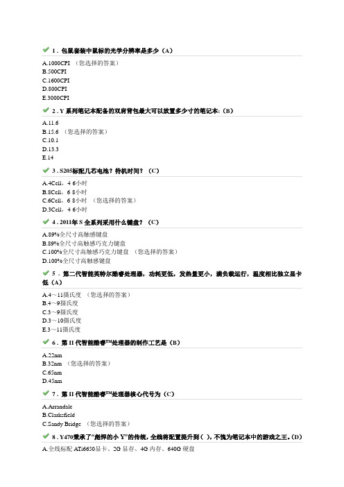
1 . 包鼠套装中鼠标的光学分辨率是多少(A)A.1000CPI (您选择的答案)B.500CPIC.1600CPID.800CPIE.3000CPI2 . Y系列笔记本配备的双肩背包最大可以放置多少寸的笔记本:(B)A.11.6B.15.6 (您选择的答案)C.10.1D.13.3E.143 . S205标配几芯电池?待机时间?(C)A.4Cell,4-6小时B.8Cell,6-8小时C.6Cell,6-8小时(您选择的答案)D.3Cell,4-6小时4 . 2011年S全系列采用什么键盘?(C)A.89%全尺寸高触感键盘B.89%全尺寸高触感巧克力键盘C.100%全尺寸高触感巧克力键盘(您选择的答案)D.100%全尺寸高触感键盘5 . 第二代智能英特尔酷睿处理器,功耗更低,发热量更小,满负载运行,温度相比独立显卡低(A)A.4~11摄氏度(您选择的答案)B.4~9摄氏度C.3~9摄氏度D.3~10摄氏度E.3~11摄氏度6 . 第II代智能酷睿™处理器的制作工艺是(B)A.22nmB.32nm (您选择的答案)C.65nmD.45nm7 . 第II代智能酷睿™处理器核心代号为(C)A.ArrandaleB.ClarksfieldC.Sandy Bridge (您选择的答案)8 . Y470秉承了“彪悍的小Y”的传统,全线将配置提升到(),不愧为笔记本中的游戏之王。
(D)A.全线标配ATi6650显卡、2G显存、4G内存、640G硬盘B.全线标配GT550显卡、1G显存、2G内存、500G硬盘C.全线标配A Ti6650显卡、1G显存、2G内存、640G硬盘D.全线标配GT550显卡、2G显存、4G内存、640G硬盘(您选择的答案)9 . ideaCenterB320支持________,可以边聊天,边看电视(B)A.一键电视技术B.PC/TV画中画(您选择的答案)C.多线程技术10 . ideaCenterB320最大支持______的硬盘和_______的内存?A.2TB 7200rpm 笔记本硬盘,8GB DDR3 1333MHz SO-DIMMB.2TB 7200rpm 台式硬盘,4GB DDR3 1333MHz SO-DIMM (您选择的答案)C.1TB 7200rpm 笔记本硬盘,8GB DDR3 1333MHz SO-DIMMD.1TB 7200rpm 台式硬盘,4GB DDR3 1333MHz SO-DIMM11 . 英特尔最新的CPU与GPU整合平台正确的描述是A.intel Sandy Bridge 技术平台,CPU与GPU完全融合,实现效率与资源整合的最优化B.intel APU技术平台,真正将CPU与GPU完美的融合在一起,实现效率与资源整合的最优化(您选择的答案)C.intel Westmere – Clarkdale 技术平台,多芯片封装方案,实现效率与资源整合的最优化12 . B520的服务保修描述正确的是哪个?(D)A.两年保修,两年上门服务B.两年保修,无上门服务C.三年保修,一年上门服务D.三年保修,三年上门服务(您选择的答案)13 . C205一体机采用多大的屏幕(D)A.20WB.19WC.21.5WD.18.5W (您选择的答案)14 . LeOS2.0是基于Android哪个版本核心研发的?(C)A.2B.3C.2.2 (您选择的答案)D.1.615 . 乐Pad屏幕尺寸是_____,分辨率为_____加上_____的宽高比,浏览网页内容更多,观看视频更爽。
intel cpu型号大全

intel cpu型号大全2009年12月24日星期四 15:12intel cpu型号大全按照处理器支持的平台来分,Intel处理器可分为台式机处理器、笔记本电脑处理器以及工作站/服务器处理器三大类;下面我们将根据这一分类为大家详细介绍不同处理器名称的含义与规格。
由于Intel产品线跨度很长,不少过往产品已经完全或基本被市场淘汰(比如奔腾III和赛扬II),为了方便起见,我们的介绍也主要围绕P4推出后Intel发布的处理器产品展开。
台式机处理器Pentium 4(P4)第一款P4处理器是Intel在2000年11月21日发布的P4 1.5GHz处理器,从那以后到现在近四年的时间里,P4处理器随着规格的不断变化已经发展成了具有近10种不同规格的处理器家族。
在这里面,“P4 XXGHz”是最简单的P4处理器型号。
这其中,早期的P4处理器采用了Willamette核心和Socket 423封装,具256KB二级缓存以及400MHz前端总线。
之后由于接口类型的改变,又出现了采用illamette核心和Socket478封装的 P4产品。
而目前我们所说的“P4”一般是指采用了Northwood核心、具有400MHz前端总线以及512KB二级缓存、基于Socket 478封装的P4处理器。
虽然规格上不一样,不过这些处理器的名称都采用了“P4 XXGHz”的命名方式,比如P4 1.5GHz、P4 1.8GHz、P4 2.4GHz。
Pentium 4 A(P4 A)有了P4作为型号基准,那么P4 A就不难理解了。
在基于Willamette核心的P4处理器推出后不久,Intel为了提升处理器性能,发布了采用Northwood 核心、具有 400MHz前端总线以及512KB二级缓存的新一代P4。
由于这两种处理器在部分频率上发生了重叠,为了便于消费者辨识,Intel就在出现重叠的、基于Northwood核心的P4处理器后面增加一个大写字母“A”以示区别,于是就诞生了P4 1.8A GHz、P4 2.0A GHz这样的处理器产品。
计算机组成与设计第五版答案
计算机组成与设计:《计算机组成与设计》是2010年机械工业出版社出版的图书,作者是帕特森(DavidA.Patterson)。
该书讲述的是采用了一个MIPS 处理器来展示计算机硬件技术、流水线、存储器的层次结构以及I/O 等基本功能。
此外,该书还包括一些关于x86架构的介绍。
内容简介:这本最畅销的计算机组成书籍经过全面更新,关注现今发生在计算机体系结构领域的革命性变革:从单处理器发展到多核微处理器。
此外,出版这本书的ARM版是为了强调嵌入式系统对于全亚洲计算行业的重要性,并采用ARM处理器来讨论实际计算机的指令集和算术运算。
因为ARM是用于嵌入式设备的最流行的指令集架构,而全世界每年约销售40亿个嵌入式设备。
采用ARMv6(ARM 11系列)为主要架构来展示指令系统和计算机算术运算的基本功能。
覆盖从串行计算到并行计算的革命性变革,新增了关于并行化的一章,并且每章中还有一些强调并行硬件和软件主题的小节。
新增一个由NVIDIA的首席科学家和架构主管撰写的附录,介绍了现代GPU的出现和重要性,首次详细描述了这个针对可视计算进行了优化的高度并行化、多线程、多核的处理器。
描述一种度量多核性能的独特方法——“Roofline model”,自带benchmark测试和分析AMD Opteron X4、Intel Xeo 5000、Sun Ultra SPARC T2和IBM Cell的性能。
涵盖了一些关于闪存和虚拟机的新内容。
提供了大量富有启发性的练习题,内容达200多页。
将AMD Opteron X4和Intel Nehalem作为贯穿《计算机组成与设计:硬件/软件接口(英文版·第4版·ARM版)》的实例。
用SPEC CPU2006组件更新了所有处理器性能实例。
图书目录:1 Computer Abstractions and Technology1.1 Introduction1.2 BelowYour Program1.3 Under the Covers1.4 Performance1.5 The Power Wall1.6 The Sea Change: The Switch from Uniprocessors to Multiprocessors1.7 Real Stuff: Manufacturing and Benchmarking the AMD Opteron X41.8 Fallacies and Pitfalls1.9 Concluding Remarks1.10 Historical Perspective and Further Reading1.11 Exercises2 Instructions: Language of the Computer2.1 Introduction2.2 Operations of the Computer Hardware2.3 Operands of the Computer Hardware2.4 Signed and Unsigned Numbers2.5 Representing Instructions in the Computer2.6 Logical Operations2.7 Instructions for Making Decisions2.8 Supporting Procedures in Computer Hardware2.9 Communicating with People2.10 ARM Addressing for 32-Bit Immediates and More Complex Addressing Modes2.11 Parallelism and Instructions: Synchronization2.12 Translating and Starting a Program2.13 A C Sort Example to Put lt AU Together2.14 Arrays versus Pointers2.15 Advanced Material: Compiling C and Interpreting Java2.16 Real Stuff." MIPS Instructions2.17 Real Stuff: x86 Instructions2.18 Fallacies and Pitfalls2.19 Conduding Remarks2.20 Historical Perspective and Further Reading2.21 Exercises3 Arithmetic for Computers3.1 Introduction3.2 Addition and Subtraction3.3 Multiplication3.4 Division3.5 Floating Point3.6 Parallelism and Computer Arithmetic: Associativity 3.7 Real Stuff: Floating Point in the x863.8 Fallacies and Pitfalls3.9 Concluding Remarks3.10 Historical Perspective and Further Reading3.11 Exercises4 The Processor4.1 Introduction4.2 Logic Design Conventions4.3 Building a Datapath4.4 A Simple Implementation Scheme4.5 An Overview of Pipelining4.6 Pipelined Datapath and Control4.7 Data Hazards: Forwarding versus Stalling4.8 Control Hazards4.9 Exceptions4.10 Parallelism and Advanced Instruction-Level Parallelism4.11 Real Stuff: theAMD OpteronX4 (Barcelona)Pipeline4.12 Advanced Topic: an Introduction to Digital Design Using a Hardware Design Language to Describe and Model a Pipelineand More Pipelining Illustrations4.13 Fallacies and Pitfalls4.14 Concluding Remarks4.15 Historical Perspective and Further Reading4.16 Exercises5 Large and Fast: Exploiting Memory Hierarchy5.1 Introduction5.2 The Basics of Caches5.3 Measuring and Improving Cache Performance5.4 Virtual Memory5.5 A Common Framework for Memory Hierarchies5.6 Virtual Machines5.7 Using a Finite-State Machine to Control a Simple Cache5.8 Parallelism and Memory Hierarchies: Cache Coherence5.9 Advanced Material: Implementing Cache Controllers5.10 Real Stuff: the AMD Opteron X4 (Barcelona)and Intel NehalemMemory Hierarchies5.11 Fallacies and Pitfalls5.12 Concluding Remarks5.13 Historical Perspective and Further Reading5.14 Exercises6 Storage and Other I/0 Topics6.1 Introduction6.2 Dependability, Reliability, and Availability6.3 Disk Storage6.4 Flash Storage6.5 Connecting Processors, Memory, and I/O Devices6.6 Interfacing I/O Devices to the Processor, Memory, andOperating System6.7 I/O Performance Measures: Examples from Disk and File Systems6.8 Designing an I/O System6.9 Parallelism and I/O: Redundant Arrays of Inexpensive Disks6.10 Real Stuff: Sun Fire x4150 Server6.11 Advanced Topics: Networks6.12 Fallacies and Pitfalls6.13 Concluding Remarks6.14 Historical Perspective and Further Reading6.15 Exercises7 Multicores, Multiprocessors, and Clusters7.1 Introduction7.2 The Difficulty of Creating Parallel Processing Programs7.3 Shared Memory Multiprocessors7.4 Clusters and Other Message-Passing Multiprocessors7.5 Hardware Multithreading 637.6 SISD,MIMD,SIMD,SPMD,and Vector7.7 Introduction to Graphics Processing Units7.8 Introduction to Multiprocessor Network Topologies7.9 Multiprocessor Benchmarks7.10 Roofline:A Simple Performance Model7.11 Real Stuff:Benchmarking Four Multicores Using theRooflineMudd7.12 Fallacies and Pitfalls7.13 Concluding Remarks7.14 Historical Perspective and Further Reading7.15 ExercisesInuexC D-ROM CONTENTA Graphics and Computing GPUSA.1 IntroductionA.2 GPU System ArchitecturesA.3 Scalable Parallelism-Programming GPUSA.4 Multithreaded Multiprocessor ArchitectureA.5 Paralld Memory System G.6 Floating PointA.6 Floating Point ArithmeticA.7 Real Stuff:The NVIDIA GeForce 8800A.8 Real Stuff:MappingApplications to GPUsA.9 Fallacies and PitflaUsA.10 Conduding RemarksA.1l HistoricalPerspectiveandFurtherReadingB1 ARM and Thumb Assembler InstructionsB1.1 Using This AppendixB1.2 SyntaxB1.3 Alphabetical List ofARM and Thumb Instructions B1.4 ARM Asembler Quick ReferenceB1.5 GNU Assembler Quick ReferenceB2 ARM and Thumb Instruction EncodingsB3 Intruction Cycle TimingsC The Basics of Logic DesignD Mapping Control to HardwareADVANCED CONTENTHISTORICAL PERSPECTIVES & FURTHER READINGTUTORIALSSOFTWARE作者简介:David A.Patterson,加州大学伯克利分校计算机科学系教授。
硬件测试专家HWiNFO
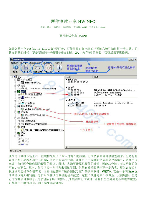
硬件测试专家HWiNFO作者:佚名转贴自:本站原创点击数:4667 文章录入:admin硬件测试专家HWiNFO如果您是一个DIY(Do It Yourself)爱好者,可能需要对你电脑的“五脏六腑”知道得一清二楚。
尤其在超频的时候,更是要搞清一些硬件(例如主板、CPU、内存等)的参数,否则后果不堪设想。
现在的计算机市场上有一些硬件采取了“瞒天过海”的招数,有的从表面就可以鉴别出来,但是有的表面上与正品看不出什么区别,实质上却大相径庭,在使用了一段时间之后就会“露馅”,这样不仅麻烦,有时还会造成别的硬件的损坏。
所以,去购买计算机硬件的时候,可能总会担心商家给你的货不真、价不实。
这时,您可以找一些行家来帮忙鉴别。
但是有时候眼见却不一定为实,那怎么办呢?我这里向您推荐个很有名、很流行的堪称“硬件测试专家”的共享软件:HWiNFO。
它是一个叫Martin 的斯洛伐克人编写的,专门用来测试计算机的硬件配置。
这位“硬件专家”很专业,只测硬件,但是它的检测项目多极了,几乎包括了所有硬件,几乎能测所有的硬件:计算机里里外外的各种硬件配置,它都能一一测试出来,而且结果非常详细。
还可以得出本机CPU与别的机器之间的差异HWiNFO给人总的印象是:一个小巧玲珑、功能强大的硬件测试工具,足以抵挡任何电脑硬件配备信息基准测试软件,您机器里的所有硬件都将在它慧眼下暴露无遗,还能对CPU、硬盘、显卡等进行分值测试,对测试结果进行综合报告,为您提供您计算机中所有硬件设备的重要信息,而不用动辄拆开机箱来查看。
而且使用起来很简单、快速,在大多数计算机硬件系统上都很有效,是一般的计算机用户或者DIY必备的工具。
识别你的内存真面目对一般用户来说,凭肉眼是很难分辨内存条是否完好。
商家有可能会把一个普通牌子的内存打磨后充当另一个牌来卖,也有可能将二手货打磨后当新货卖给你。
用HWINFO就可以检测出你所购内存的详细资料,其它HWINFO除了测内存外还可以测主板和CPU 等配件。
卫星列表

Western HemisphereLocation Satellite SatellitebusSourceOperator TypeCoverageLaunchdate/rocket(GMT)AlllocationsRemarksAs of148.0°W EchoStar-1LockheedMartinAS-7000USEchostar/DISHNetworkDirectBroadcasting28December1995, LongMarch 2E119°W(1996-1999),148.0°W(1999—)Scheduled to moveto 77°Wsoon2009-02-06139.0°W Americom-8LockheedMartinA2100AUSSES Americom& AT&TAlascomTelevisionand radiobroadcasting24 Cband(Canada,Caribbean,mainlandUSA)19December2000,Ariane 5GPreviouslyGE-8 forGEAmericom; alsoknown asAurora III;replacedSatcomC-5 inMarch20012008-11-20137.0°W Americom-7LockheedMartinUS SES AmericomTelevisionand radioMainlandUSA,14SeptemberPreviouslyGE-7 for2008-11-20A2100A broadcasting Canada,Mexico2000,Ariane 5GGEAmericom135.0°W Americom-10LockheedMartinA2100AUS SES AmericomTelevisionand RadioBroadcastingMainlandUSA,Canada,Caribbean, Mexico5 February2004, AtlasII AS2008-11-20133.0°W Galaxy-12 OrbitalSciencesCorporationStar-2US IntelsatTelevision/RadioBroadcasting9 April2003,Ariane 5G123.0°WreplacedfailedGalaxy 15131.0°W Americom-11LockheedMartinA2100AUS SES AmericomTelevisionand RadioBroadcasting24C-BandTranspondersMainlandUSA,Canada,Caribbean, Mexico19 May2005, AtlasII AS2008-11-20129.0°W Galaxy-27SpaceSystems/Loral FS-1300US IntelsatTelevisionbroadcasting & SatelliteInternetAccess25September1999,Ariane 44LPFormerlyknown asIA-7 andTelstar-72008-11-20Ciel-2ThalesAlenia SpaceSpacebus4000 C4CanadaCiel SatelliteGroupDirectBroadcasting10December2008,Proton-MLeased toEchostar/DishNetwork2009-02-06127.0°W Galaxy-13BoeingBSS-601US Intelsat24C-Bandtransponders1 October2003,Zenit-3SLSamesatelliteasHorizons-12008-11-20Horizons-1BoeingBSS-601USJapan SatelliteSystems24Ku-Bandtransponders1 October2003,Zenit-3SLSamesatelliteasGalaxy-132008-11-20125.0°W Galaxy-14 OrbitalSciencesCorporationStar-2US Intelsat24C-Bandtransponders -NorthAmerica13 August2005,Soyuz-FG/Fregat2008-11-20123.0°W Galaxy-18 SpaceSystems/Loral LS-1300US IntelsatTelevisionand radiobroadcastingNorthAmerica21 May2008,Zenit-3SLHybridC/Ku-band satellite2008-11-19121.0°W Galaxy-23SpaceSystems/LorUS IntelsatDirectBroadcastinNorthAmerica7 August2003,HybridC/Ku/Ka-b2008-11-26al FS-1300 g Zenit-3SL andsatellite;C-bandpayloadreferred toasGalaxy-23EchoStar-9 SpaceSystems/Loral FS-1300USEchostar/DISHNetworkDirectBroadcastingNorthAmerica7 August2003,Zenit-3SLHybridC/Ku/Ka-bandsatellite;Ku/Ka-bandpayloadreferred toasEchoStar-92008-11-26119.0°W DirecTV-7SSpaceSystems/Loral LS-1300US DirecTVDirectBroadcasting54Ku-bandtransponders4 May 2004,Zenit-3SL8 activetransponders at thistime2008-11-26EchoStar-7LockheedMartinA2100AXUSEchostar/DISHNetworkDirectBroadcasting32Ku-bandtranspond21 February2002, AtlasIII B21 activetransponders at this2008-11-26ers time118.8°W Anik F3EADSAstriumEurostar-3000SCanada Telesat CanadaDirectBroadcasting24C-bandtransponders, 32Ku-bandtransponders, 2Ka-bandtransponders11 April2007,ProtonKu-Bandleased toEchostar/DishNetwork2008-11-26116.8°W SatMex-5HughesHS-601HPMexico Satmex24C-bandtransponders, 24Ku-bandtransponders5 December1998,Ariane 42L2008-11-26115.0°W XM-Blues US30 October2006,Zenit-3SL Solidaridad-2Mexico Satmex8 October1994,Ariane 44L113.0°W Satmex-6Mexico Satmex27 May2006, Ariane 5-ECA111.1°W Anik F2Boeing 702 Canada Telesat Canada DirectBroadcasting17 July2004,Ariane 5GHybridC/Ku/Ka-bandsatellite110.0°W EchoStar-11SpaceSystems/Loral LS-1300USEchostar/DISHNetworkDirectBroadcasting17 July2008,Zenit-3SL2008-11-19EchoStar-10A2100AXS USEchostar/DISHNetworkDirectBroadcasting15 February2006,Zenit-3SLDirecTV-5LS-1300US DirecTVDirectBroadcasting7 May 2002,Proton32Ku-bandtransponders107.3°W Anik F1Boeing 702 Canada Telesat CanadaDirectBroadcasting21November2000,Ariane 44LHybridC/Ku-band satellite;will bereplacedby AnikF1RAnik F1R Eurostar-300Canada Telesat Canada Direct 8 Hybrid0Broadcasting, WAASPRN #138 September2005,ProtonC/Ku-band satellite;willreplaceAnik F1105.0°W AMC-18A2100A US SES AmericomDirectBroadcastingMainlandUSA,Canada,Caribbean, Mexico8 December2006,Ariane 5Americom-15A2100AXS US SES AmericomDirectBroadcastingCONUS,Alaska,Hawaii15 October2004,Proton-MHybridKu/Ka-bandsatellite;twin ofAmericom-16103.0°W Americom-1A2100A US SES AmericomMainlandUSA,Canada,Mexico,Caribbean8September1996, AtlasII AHybridC/Ku-band satellite102.8°W SPACEWAY-1Boeing 702 US DirecTVDirectBroadcastin26 April2005,g Zenit-3SL101.2°W DirecTV-4SBoeing 601 US DirecTVDirectBroadcasting27November2001,Ariane 44LP48Ku-bandtransponders101.1°W DirecTV-9SLS-1300US DirecTVDirectBroadcasting13 October2006,Ariane5-ECA101.0°W AMC-4A2100AX US SES Americom MainlandUSA,Canada,Mexico,Caribbean, CentralAmerica13November1999,Ariane 44LPHybridC/Ku-band satellite100.8°W DirecTV-8LS-1300US DirecTV DirectBroadcasting22 May2005,ProtonHybridKu/Ka-bandsatellite99.2°W SPACEWAY-2US16November 2005,Ariane5-ECA99.0°W Galaxy-16FS-1300Intelsat 18 June 2006, Zenit-3SL97.0°W Galaxy-19SpaceSystems/Loral FS-1300US IntelsatTelevisionand RadioBroadcasting24 C- and28Ku-bandtransponders NorthAmerica24September2008,Zenit-3SL2008-11-2095.0°W Galaxy 3C US 15 June 2002, Zenit-3SL93.0°W Galaxy-26SSLFS-1300US15 February1999,Proton-K91.0°W Nimiq 1A2100AX Canada Telesat CanadaDirectBroadcasting20 May1999,Proton32Ku-bandtranspondersGalaxy 17Spacebus-3000B3US IntelsatTelevisionand radiobroadcastingNorthAmerica4 May 2007,Ariane5-ECA74°WJuly 2007to March2008HybridC/Ku-band satellite2008-06-1389.0°W Galaxy-28FS-1300ITSO Intelsat TheAmericas23 June2005,HybridC/Ku/Ka-bZenit-3SL andsatellite;launchedasTelstar 887.0°W AMC 3A2100A US SES Americom MainlandUSA,Canada,Mexico,Caribbean4September1997, AtlasII AHybridC/Ku-band satellite85.0°W XM-RhythmBoeing 702 USXM SatellieRadio HoldingsRadioBroadcastingCONUS28 February2005,Zenit-3SLAmericom-2A2100A US SES AmericomDirectBroadcastingMainlandUSA,Canada,Mexico30 January1997,Ariane 44LAmericom-16A2100AXS US SES AmericomDirectBroadcastingCONUS,Alaska,Hawaii17December2004, AtlasV (521)HybridKu/Ka-bandsatellite;twin ofAmericom-1584.0°W Brasilsat-B3Brazil4 February1998,Ariane 44LP83.0°W Americom-93000B3US SES AmericomDirectBroadcastingCONUS,Canada,Mexico,CentralAmerica,Caribbean7 June2003,ProtonHybridC/Ku-band satellite82.0°W Nimiq 2A2100AX Canada Telesat CanadaDirectBroadcasting29December2002,ProtonHybridKu/Ka-bandsatellite Nimiq 3HS-601Telesat CanadaDirectBroadcasting9 June1995,Ariane 42PPreviouslyDirecTV-3forDirecTV80.9°W SBS-6HS-393 US Intelsat Televisionand RadioBroadcasting12 October1990,Ariane 44L74°WNov 1995to Jan2008Beyondexpectedend of life.ServesArgentinanow2008-06-1379.0°W Americom Spacebus-20US SES Americom CONUS, 28 October-500 Canada,Mexico 1998, Ariane 44LSatcom C3US10September1992,Ariane 44LPInclinedorbit77.0°W EchoStar-4A2100AX USEchostar/DISHNetworkDirectBroadcasting8 May 1998,ProtonspareEchoStar-8FS-1300USEchostar/DISHNetworkDirectBroadcasting21 August2002,Proton110°W2008-11-1976.8°W Galaxy 4R US 19 April2000,Ariane 42LInclinedorbit75.0°W Brasilsat-B1Brazil10 August1994,Ariane 44LP74.9°W Galaxy-9US 24 May1996, DeltaII (7925)spare74.0°W Horizons-2STAR Bus US Intelsat JSATTelevisionand RadioBroadcastingCONUSCanadaCaribbean21December2007,Ariane 5GS20 KuXpndrs2008-06-1372.7°W EchoStar-6FS-1300USEchostar/DISHNetworkDirectBroadcasting14 July2000, AtlasII AS2008-11-1972.5°W Directv-1R US 10 October 1999, Zenit-3SL72.0°W AMC-6A2100AX US SES Americom CONUS,Canada,Mexico,Caribbean, CentralAmerica22 October2000,Proton-MHybridC/Ku-band satellite;a portionof theKu-bandpayload isdedicatedto SouthAmerica71.0°W Nahuel-1A Argentina30 January1997,Ariane 44L70.0°W Brasilsat-B4Brazil17 August2000,Ariane 44LP65.0°W Brasilsat-B2Brazil28 March1995,Ariane44LP+63.0°W Estrela doSul 1Brazil11 January2004,Zenit-3SL61.5°W EchoStar-12A2100AXS US17 July2003, AtlasV (521)FormerlyRainbow-1,purchased fromVOOM EchoStar-3A2100AX USEchostar/DISHNetworkDirectBroadcasting5 October1997, AtlasII AS61.0ºW HispasatAmazonasSpain4 August2004,Proton-M58.0°W Intelsat-9HS601HP US 28 July2000,Zenit-3SLformerlyPAS-955.5°W Intelsat-805ITSO18 June1998, AtlasII AS53.0°W Intelsat-707ITSO14 March1996,Ariane 450.0°W Intelsat-705ITSO22 March1995, AtlasII AS45.0°W Intelsat-1RHS702 US16November2000,Ariane 5GformerlyPAS-1R43.1°W Intelsat-3RHS601 US12 January1996,Ariane 44LformerlyPAS-3R43.0°W Intelsat-6BHS601HP22December1998,Ariane 42LformerlyPAS-6B40.5°W NSS-806LM AS-7000 Netherlands28 February1998, AtlasII AS37.5°W NSS-10Spacebus4000C33 February2005,ProtonTelstar-11USInclinedorbit34.5°W Intelsat-903ITSO30 March2002,Proton-K31.5°W Intelsat-801ITSO1 March1997,Ariane 44P30.0°W Hispasat-1CSpain3 February2000, AtlasII ASHispasat-1DSpain18September2002, AtlasII AS27.5°W Intelsat-907ITSO15 February2003,Ariane 44L24.5°W Intelsat-905ITSO5 June2002,Ariane 44L24.0°W Cosmos2379RussiaInclinedorbit22.0°W NSS-7LM A2100AX Netherlands16 April2002,Ariane 44L20.0°W Intelsat-603ITSO14 March1990,CommercialTitan IIIInclinedorbit18.0°W Intelsat-901ITSO9 June2001,Ariane 44L15.5°W Inmarsat 3F2IMSOEGNOSPRN #1206September1996,Proton-K15.0°W Telstar 12SSL US 19 October 1999, Ariane 44LP14.0°W Gorizont32RussiaInclinedorbit Express-A4Russia12.5°W AtlanticBird 1EUMETSAT28 August2002,Ariane 5G11.0°W Express-A3Russia24 June2000,Proton-K8.0°W AtlanticBird 2Eutelsat25September2001,Ariane 44PTelecom 2D France8 August1996,Ariane 44LInclinedorbit7.0°W Nilesat101Egypt28 April1998,Ariane 44P Nilesat102Egypt17 August2000,Ariane 44LP Nilesat103Egypt27 February1998,Ariane 42P AtlanticBird 4Eutelsat27 February1998,Ariane 42P5.0°W AtlanticBird 3Eutelsat4.0°W AMOS 1Israel16 May1996,Ariane 44L AMOS 2Israel27December2003,Soyuz-FG/Fregat3.4°W Meteosat828 August2002,Ariane 5G1.0°W Intelsat10-02ITSO16 June2004,Proton-M0.8°W Thor 2Norway20 May1997, DeltaIIThor 3Norway10 June1998, DeltaII (7925-9.5)[edit] Eastern HemisphereLocation Satellite SatellitebusSource Operator TypeCoverageLaunchdate/rocket(GMT)AlllocationsRemarks As of0.5°E Meteosat7ESAWeathersatellite2September1997,Ariane 44LPInclinedorbit3.0°E Telecom2A16December1991,Ariane 44L4.0°E Eurobird 4Eutelsat 2 September 1997, Ariane 44LP4.8°E Sirius 4A2100AX Sweden SES Sirius Comsat52Ku-bandcoveringEurope2Ka-bandcoveringScandinavia17November2007,Proton M2007-11-18 Astra 1CLuxembourg12 May1993,Ariane 42L0.9°inclinedorbit5.0°E Sirius 3Sweden 5 October 1998, Ariane 44L5.2°E Astra 1A GE 4000 11 December 1988, Ariane 44LP6.0°E Skynet 4F Militarycommunica7 February2001,Inclinedorbittions Ariane 44L7.0°E EutelsatW3AEutelsat15 March2004,Proton-M9.0°E Eurobird 9Eutelsat 21November1996, AtlasII AformerlyHot Bird 29.5°E Meteosat6ESAWeathersatellite20November1993,Ariane 44LPInclinedorbit10.0°E EutelsatW1Eutelsat6September2000,Ariane 44P12.5°E Raduga29RussiaInclinedorbit13.0°E Hot Bird 6Eutelsat21 August2002, AtlasV (401)Hot Bird7AEutelsat11 March2006,Ariane5-ECAHot Bird 8Eutelsat 4 August 2006, Proton16.0°E EutelsatW2Eutelsat5 October1998,Ariane 44L19.2°E Astra 1ELuxembourg19 October1995,Ariane 42L Astra 1FLuxembourg8 April1996,Proton-K Astra 1GLuxembourg12November1997,Proton-K Astra 1HLuxembourg18 June1999,Proton-K Astra 1KRLuxembourg20 April2006, AtlasV (411) Astra 1LLuxembourg4 May 2007,Ariane5-ECA20.0°E Arabsat2A9 July 1996,Ariane 44LInclinedorbit21.0°E AfriStar US 28 October 1998, Ariane 44L21.5°E EutelsatW6Artemis ESAEGNOSPRN #12412 July2001,Ariane 5GInclinedorbit.23.5°E Astra 3A Luxembourg29 March2002,Ariane 44L25.0°E Inmarsat 3F5IMSOEGNOSPRN #1264 February1998,Ariane 44LP25.5ºE Eurobird 2Eutelsat25.8°E Badr 226.0°E Badr 326.2°E Badr C28.2°E Astra 2A HS601HPLuxembourgAstra 2BLuxembourg14September2000, Ariane 5GAstra 2C Luxembourg16 June2001,Proton-KAstra 2D Luxembourg20December2000,Ariane 5G28.5°E Eurobird 1Spacebus3000Eutelsat8 March2001,Ariane 5G30.5°E Arabsat2BArabsat13November1996,Ariane 44L31.3°E Astra 1D HS-601LuxembourgSES Astra Comsat24Ku-band1 November1994,Ariane 419.2°E(1994–1998)28.2°E(1998)19.2°E(1998–1999)28.2°E2007-11-14(1999–2001)24.2°E(2001–2003)23.0°E(2003–2004)23.5°E(2004–2007)30.0°E(2007—) 31.5°E Sirius 2Sweden33.0°E Eurobird 3Eutelsat27September2003,Ariane 5G Intelsat802LM-3000 ITSO25 June1997,Ariane 44P36.0°E EutelsatSesat 1Eutelsat17 April2000,Proton-K Eutelsat Eutelsat24 May。
28270735
旁边 还 为计 算器 程 序单独 提 供 了快 捷 键 。 当然 , 所有这 些 快 捷 键 都可 以根 据 自
己 的 习 惯 进 行 自定 义 , 这 在 驱 动 程 序 界 面 中可 以很 容 易地 完 成 。 除 了这 些 之 外 , 该 产 品 还 提 供 了 多个 出水 孔 , 可 以 在 意 外 发 生 时最大限 度地 减 少损 失 。 口
厂商 电话
微 软 ( 中国 ) 有限 公 司
80 0 — 8 20— 3 800
网址
h t t p //w w w m ic r o s o f t c o rn
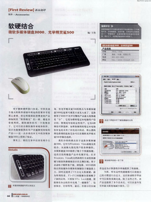
对 于 微软硬 件部 门来说 , 尽管在这
个庞大 的软件帝国 中所处 的位置 并不是
那么重 要 , 但它所提 供给 消费者的产 品 却如 同其 “ 软 件 师 兄 ” 们 一 样 , 都 是 非
盘 3 0 0 0 比起 来可 就 是小巫 见大巫 了 , 这 款
使 用 了8 0 0 D P I 光 学 引擎 的产 品 最 大 优 势 就
是 小 “
”
, 它是为那些笔记本电脑用户设
计 的 , 特 别 是 年 轻 的女 性 用 户 。 它 有6 种
颜色可 供选择 , 如果你使用 的笔记本 电脑
恰 好也 是采 用 了彩壳设计 的话 , 那 么 想找
[F i r s t R e v i e w ] 新 品 初 i乎
附件 。 A c c e s s o r ie s
软硬 结 合
微软 多媒 体键盘 3 0 0 0 、 光学精 灵 鲨 5 0 0
重庆维普
编 /王 欣
产品信息
价格
2 9 9 元 /1 2 9 元
常优 秀的 。 微软硬 件的 另一 个优 势在
AMD Reference Configuration for Ansys on Dell Powe
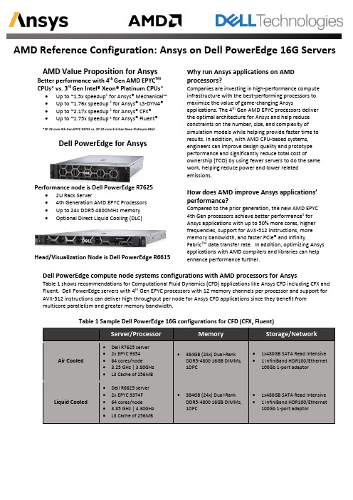
AMD Reference Configuration: Ansys on Dell PowerEdge 16G ServersAMD Value Proposition for AnsysBetter performance with 4th Gen AMD EPYC TM CPUs * vs. 3rd Gen Intel® Xeon® Platinum CPUs *• Up to ~1.5x speedup 1for Ansys® Mechanical™ • Up to ~1.76x speedup 2 for Ansys® LS-DYNA® • Up to ~2.17x speedup 3 for Ansys® CFX® •Up to ~1.75x speedup 4 for Ansys® Fluent®*2P 32-core 4th Gen EPYC 9374F vs. 2P 32-core 3rd Gen Xeon Platinum 8362Dell PowerEdge for AnsysPerformance node is Dell PowerEdge R7625• 2U Rack Server• 4th Generation AMD EPYC Processors • Up to 24x DDR5 4800MHz memory •Optional Direct Liquid Cooling (DLC)Head/Visualization Node is Dell PowerEdge R6615Why run Ansys applications on AMD processors?Companies are investing in high-performance compute infrastructure with the best-performing processors to maximize the value of game-changing Ansysapplications. The 4th Gen AMD EPYC processors deliver the optimal architecture for Ansys and help reduce constraints on the number, size, and complexity of simulation models while helping provide faster time to results. In addition, with AMD CPU-based systems, engineers can improve design quality and prototype performance and significantly reduce total cost ofownership (TCO) by using fewer servers to do the same work, helping reduce power and lower related emissions.How does AMD improve Ansys applications’ performance?Compared to the prior generation, the new AMD EPYC 4th Gen processors achieve better performance 5 for Ansys applications with up to 50% more cores, higher frequencies, support for AVX-512 instructions, more memory bandwidth, and faster PCIe® and InfinityFabric TM data transfer rate. In addition, optimizing Ansys applications with AMD compilers and libraries can help enhance performance further.Dell PowerEdge compute node systems configurations with AMD processors for AnsysTable 1 shows recommendations for Computational Fluid Dynamics (CFD) applications like Ansys CFD including CFX and Fluent. Dell PowerEdge servers with 4th Gen EPYC processors with 12 memory channels per processor and support for AVX-512 instructions can deliver high throughput per node for Ansys CFD applications since they benefit from multicore parallelism and greater memory bandwidth.Table 1 Sample Dell PowerEdge 16G configurations for CFD (CFX, Fluent)Table 2: Sample Dell PowerEdge 16G configurations for Structural Mechanics: Ansys MechanicalTable 3 shows recommendations for crash applications using explicit FEA like Ansys LS-DYNA. Dell PowerEdge systems with medium core count EPYC processors with high frequencies and high cache- per- -core and support for AVX-512 instructions offer very high performance per core to help efficiently utilize per-core software licenses.Table 3: Sample Dell PowerEdge 16G configurations for Explicit Finite Element Analysis (FEA): Ansys LS-DYNA Benefits: AMD CPU-based Dell PowerEdge servers with Ansys•Validated and optimized solution with compute, storage, software, services, and financial options.•On-site install, start-up, and integration services delivered by Dell Technologies or a certified Dell Technologies business partner.•Remote management is available with proactive monitoring and remediation of any Ansys operational issues. Key ContactsMary BassDISCLAIMER:The information contained herein is for informational purposes only and is subject to change without notice. While every precaution has been taken in the preparation of this document, it may contain technical inaccuracies, omissions, and typographical errors, and AMD is under no obligation to update or otherwise correct this information. Advanced Micro Devices, Inc. makes no representations or warranties with respect to the accuracy or completeness of the contents of this document and assumes no liability of any kind, including the implied warranties with respect to the operation or use of AMD hardware, software or other products described herein. No license, including implied or arising by estoppel, to any intellectual property rights is granted by this document, Terms and limitations applicable to the purchase or use of AMD’s products are as set forth in a signed agreement between the parties or in AMD’s Standard Terms and Conditions of Sale.COPYRIGHT NOTICE©2023 Advanced Micro Devices, Inc. All rights reserved. AMD Arrow logo, AMD Instinct, EPYC, Infinity Fabric, and combinations thereof are trademarks of Advanced Micro Devices, Inc. Ansys, CFX, Fluent, LS-DYNA, Mechanical, and any and all Ansys, Inc. brand, product, service and feature names, logos and slogans are registered trademarks or trademarks of Ansys, Inc. or its subsidiaries in the United States or other countries under license. PCIe is a registered trademark of PCI-SIG Corporation. Other product names used in this publication are for identification purpose only and may be trademarks of their respective companies. .1 SP5-130: Mechanical® Release 2022 R2 test cases benchmarkcomparison based on AMD measurements as of 10/19/2022. Configurations: 2x 32-core Intel Xeon Platinum 8362 vs. vs. 2x 32-core EPYC 9374F for ~1.5x the rating performance. System Configurations:2P AMD EPYC 9374F (32 cores/socket, 64 cores/node); 1.5 TB (24x) Dual-Rank DDR5-4800 64GB DIMMs, 1DIMM per channel; 1 x 256 GB SATA (OS) | 1 x 1 TB NVMe (data); BIOS Version 1002, SMT=off, Determinism=performance, NPS=4, TDP/ PPT=400; RHEL 8.6; OS settings:Clear caches before every run, NUMA balancing 0, randomize_va_space 0 vs. 2P Intel Xeon Platinum 8362 (32 cores/socket, 64 cores/node); 1 TB (16x) Dual-Rank DDR4-3200 64GB DIMMs, 1DIMM per channel; 1 x 256 GB SATA (OS) | 1 x 1 TB NVMe (data); BIOS Version1.6.5, SMT=off, HPC Profile; OS settings: Clear caches before every run, NUMA balancing 0, randomize_va_space 0. Results may vary based on factors such as software version, hardware configurations and BIOS version and settings.2 SP5-112: LS-DYNA® Version 2021 R1 Nonlinear FEA benchmark comparison based on AMD measurements as of 09/18/2022. Tests run: obd10m, car2car, obd10m-short, ls-3cars and ls-neon. System Configurations: 2P AMD EPYC 9374F (32 cores/socket, 64 cores/node); 1.5 TB (24x) Dual-Rank DDR5-4800 64GB DIMMs, 1DIMM per channel; 1 x 256 GB SATA (OS) | 1 x 1 TB NVMe (data); BIOS Version 1002C, SMT=off, Determinism=performance, NPS=4, TDP/ PPT=400 versus 2P Intel Xeon Platinum 8362 (32 cores/socket, 64 cores/node); 1 TB (16x) Dual-Rank DDR4-3200 64GB DIMMs, 1DIMM per channel; 1 x 256 GB SATA (OS) | 1 x 1 TB NVMe (data); BIOS Version 1.6.5,SMT=off, HPC Profile. Common: RHEL 8.6 OS settings: Clear caches before every run, NUMA balancing 0, randomize_va_space 0. Results may vary due to factors including system configurations, software versions and BIOS settings.3 SP5-116: CFX 2022 R2 Solver, Nonlinear CFD benchmark comparison based on AMD measurements as of 9/16/22. Tests used: cfx_100, cfx_50, cfx_10, cfx_lmans, cfx_pump. Configurations: 2P AMD EPYC 9374F (32 cores/socket, 64 cores/node); 1.5 TB (24x) Dual-Rank DDR5-4800 64GB DIMMs, 1DIMM per channel; 1 x 256 GB SATA (OS) | 1 x 1 TB NVMe (data); BIOS Version 1002C, SMT=off, Determinism=performance, NPS=4, TDP/ PPT=400 versus 2P Intel Xeon Platinum 8362 (32 cores/socket, 64 cores/node); 1 TB (16x) Dual-Rank DDR4-3200 64GB DIMMs, 1DIMM per channel; 1 x 256 GB SATA (OS) | 1 x 1 TB NVMe (data); BIOS Version 1.6.5, SMT=off, HPC Profile. Common: RHEL 8.6 OS settings: Clear caches before every run, NUMA balancing 0, randomize_va_space 0. Results may vary due to factors including system configurations, software versions and BIOS settings. 4SP5-035A: Fluent® Release 2022 R2 test cases benchmark comparison based on AMD measurements as of 10/19/2022. Configurations: 2x 32-core Intel Xeon Platinum 8362 vs. vs. 2x 32-core EPYC 9374F for ~1.75x the rating performance. Results may vary. 5https:///system/files/documents/epyc-9004-pb-ansys-generational.pdf。
MultiCore2013

更好
533/667 MHz 2 MB 最高 1.83 GHz T5000
最好
533/667 MHz 4 MB 最高 2.33 GHz T7000
ቤተ መጻሕፍቲ ባይዱ
内存 (DDR2)
芯片组 无线
最高 667 MHz
最高 667 MHz
最高 667 MHz
移动式英特尔® 945 高速芯片组家族 英特尔® PRO/无线 3945ABG
• 计算机和处理器的发展历程 • 计算机诞生初期,程序指令是存储在内存 中顺序执行的。 • 上世纪60年代,多个用户可以同时访问同一 台大型机,并发出现. • 早期的个人电脑,单用户操作系统,同一时刻 只能运行一个程序. • 近期,互联网开始普及.用户需求越来越复杂, 对计算机性能的要求越来越高.
基本概念
• 指令流(instruction stream) –指机器执行的指令序列 • 数据流(data stream) –指指令流调用的数据序列,包括输入数据和中间结果。
并行计算机的分类
• 1966年由Flynn提出的分类法,称为Flynn分类法。 –单指令流单数据流(Single Instruction stream Single Data stream, SISD); –单指令流多数据流(Single Instruction stream Multiple Data stream, SIMD); –多指令流单数据流(Multiple Instruction stream Single Data stream, MISD); –多指令流多数据流(Multiple Instruction stream Multiple Data stream, MISD)。 SISD就是普通的顺序处理的串行机。SIMD和MIMD是 典型的并行计算机。MISD在实际中代表何种计算机, 也存在不同的看法,甚至有学者认为根本不存在MISD 。有的文献把流水线结构的计算机看成MISD结构。
MPC5777M 微处理器说明文档说明书

Built on 4th generation Power Architecture® e200z7 cores
Industry standard GTM (Generic Timer Module)
HSM (Hardware Security Module)
• User programmable security core with secure memory • Compliant with EVITA security specification
Package 416 TEPBGA 512 TEPBGA 512 Emulation DeCQ100 Grade1, Ta 125°C Ethernet, CAN-FD, Flexray
Precision GTM Timers and ADC Ultra-Reliable MCU
On-chip DSP, Ethernet, Zipwire, ∑∆ ADCs and 4x faster Nexus Aurora debug
4
INTERNAL USE
NXP Automotive Powertrain MCU Products
MPC55XX
130nm
32-bit MCU 2 MB Flash
2
INTERNAL USE
MPC5777M Block Diagram
Key Features • Two independent 300 MHz Power Architecture z7 computational cores – Single 300 MHz Power Architecture z7 lockstep – Delayed lock-step for ASIL-D safety • Single I/O Core 200 MHz Power Architecture z4 core • 8M Flash with ECC • 596k total SRAM with ECC – 404k of system RAM (incls. 64k standby) – 192k of tightly coupled data RAM • 10 ΣΔ converters for knock detection, 12 SAR converters – 84 total ADC channels • GTM – 248 timer channels • eDMA controller – 128 channels
一种多核间内存公平调度模型
然 后 通 过启 发 式 算 法 求 解 , 得 到 了一 个性 能较 优 的公 平调 度 算法 F Q— S J F . 基准 s o p l e x的实 验结 果 表 明 , 相 比
F R — F C F S调度 算 法 , 平均读取延迟 比 F R — F C F S减 小 了 1 0 . 6 , 有效 验证 了提 出 的 多核 调度 模 型.
关 键 词 多 核 内 存 调 度 ; 多核调度模 型 ; 公 平 队 列 调 度 中图法分类号 T P 3 1 1 D O I 号 1 0 . 3 7 2 4 / S P . J . 1 0 1 6 . 2 0 1 3 . 0 2 1 9 1
A Mu l t i — Co r e Fa i r M e mo r y S c he d u l i ng Mo d e l
第 3 6 卷 第 1 1期 2 0 1 3年 1 1月
计
算
ห้องสมุดไป่ตู้机
学
报
V01 .3 6 No .1 1 NO V .2 O1 3
O F COM PU TER S CH I NES E J OURNAL
一
种 多核 间 内存 公 平 调 度 模 型
刘虎球 赵 鹏
t h e h e u r i s t i c a l g o r i t h m t o g e t a b e t t e r p e r f o r ma n c e o f t h e f a i r s c h e d u l i n g FQ— S J F . Th r o u g h
北 京 1 0 0 0 8 4 ) ( 清 华 大学 计 算 机 科 学 与 技 术 学 院
EMC产品荣获《WINDOWS IT PRO》杂志“2006年读者选择奖”

维普资讯
信 息 窗
中兴通讯程控交换机获评 ‘ ‘ 中国 世界名牌 ’ ’
2 0  ̄9 J , 中国国 家质检 总局 0 6 f 6E l
赛诺公司发布的报告,中 兴通讯已经超 越L ,列国产c M 手机第一位。在全 G DA
和地 区
为中兴通 讯 开拓 全 球 固网通 信市 场最 先 善掌
。
类 别 , EMC@ CL ARi i ON@ CX系列 r e
‘
奖”;在 最佳 灾难 预 防, 灾难 恢复 工具类 存 储 ( A c s)平台赢得 了 “ 最佳企 业备份, 恢 复, 存档硬 件奖”。 E 最近发布 的E A I N ut 。 l Mc cL R _ I 0 阳s 。。
市 场上
口
因 其在 W
因 其在
i n
上
,
中 心对 等 站点 。运 营 商能 以更低 一’ 。 “ … …~ … 一 … 的入 门
成本 、更 ’ 部署 cRs一 ,从 而可 以 ’ … 广泛地 。 一 1 一 … ’ 。
销售
荣
荣获
P no da 旗下 ( n o T e tn Me i ( d wsI Wi
。
年4 月发布以来,已经售出超过10 B P 0 (0・ 0B 存储容量。 12 0T ) 4
思科全球最紧凑 的每插槽4 0
2 0年8 06 月,中 兴通讯c M 手 DA
在 北京人 民 大会 堂举 行 ‘ ‘ 质量 振兴 纲要
实施 1 周年 暨质 量兴 市先进 、 中国名牌 0
CX x# 台
运 营商显著 增加 收入 ,提 高效 率 ,从 而 使 E们 获得 更高利 ,开 更好 地控 制 它们 更高利 润 】 目
高性能计算习题及答案
高性能计算练习题1、一下哪种编程方式适合在单机内并行?哪种适合在多机间并行?单机:Threading线程、OpenMP;多机:MPI。
2、例题:HPC集群的峰值计算能力:一套配置256个双路X5670处理器计算节点的HPC集群。
X5560:2.93GHz Intel XS5670 Westmere六核处理器,目前主流的Intel处理器每时钟周期提供4个双精度浮点计算。
峰值计算性能:2.93GHz*4Flops/Hz*6Core*2CPU*256节点=36003.8GFlops。
Gflops=10亿次,所以36003Gflops=36.003TFlops=36.003万亿次每秒的峰值性能。
3、Top500排名的依据是什么?High Performance Linpack(HPL)测试结果4、目前最流行的GPU开发环境是什么?CUDA5、一套配置200TFlops的HPC集群,如果用双路2.93GHz Intel westmere六核处理器X5670来构建,需要用多少个计算节点?计算节点数=200TFlops/(2*2.93GHz*6*4Flops/Hz)=14226、天河1A参与TOP500排名的实测速度是多少,效率是多少?2.57PFlops 55%7、RDMA如何实现?RDMA(Remote Direct Memory Access),数据发送接收时,不用将数据拷贝到缓冲区中,而直接将数据发送到对方。
绕过了核心,实现了零拷贝。
8、InfiniBand的最低通讯延迟是多少?1-1.3usec MPI end-to-end,0.9-1us InfiniBand latency for RDMA operations9、GPU-Direct如何加速应用程序运行速度?通过除去InfiniBand和GPU之间的内存拷贝来加速程序运行。
•GPUs provide cost effective way for building supercomputers【GPUs提供高效方式建立超级计算机】•Dense packaging of compute flops with high memory bandwidth【使用高端内存带宽的密级封装浮点计算】10、网络设备的哪个特性决定了MPI_Allreduce性能?集群大小,Time for MPI_Allreduce keeps increasing as cluster size scales,也就是说集群的规模决定了MPI_Allreduce的性能。
mmWave OTA 验证测试参考架构说明书
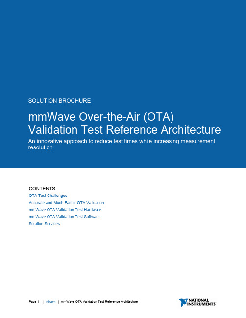
oCONTENTSOTA Test ChallengesAccurate and Much Faster OTA Validation mmWave OTA Validation Test Hardware mmWave OTA Validation Test Software Solution ServicesOTA Test Challenges5G operation at mmWave frequencies relies on beamforming technology through antenna arrays with many elements. As the industry strives to reduce the size and cost of producing these 5G beamforming devices operating at mmWave, many of them lack conventional external RF connectors, becomingintegrated Antenna-in-Package (AiP) and Antenna-in-Module (AiM) devices. This industry shift presents a tough challenge for engineers in charge of characterization and validation of integrated beamforming designs, prompting them to look for accurate, over-the-air (OTA), radiated test solutions.Test Time Challenges and Measurement UncertaintyConfiguring and running detailed 3D spatial sweeps of 5G beamforming AiP devices within a carefully controlled RF environment in an anechoic chamber can be a very time-consuming and expensive task. A typical move → stop → measure, point-by-point, software-controlled test system with a positioner that can rotate in two independent axes (azimuth and elevation), produces only a handful of RFmeasurements per second. However, engineers need to measure and validate antenna performance by scanning hundreds or even thousands of points in space. A trade-off arises, in which the finer the 3D sampling grid (smaller distance between measurement points), the higher the test times, but the lower the measurement uncertainty. Conversely, a 3D grid that is too sparse can give faster results, but introduce quite a bit of measurement error. Figure 1 illustrates how employing a 3D scanning grid to measure a DUT’s power produces a 3D antenna pattern, but the points need to be close enough to minimize resolution errors.Figure 1 Selecting a denser 3D scanning grid reduces measurement uncertaintyFurthermore, getting data at multiple frequencies and powers, and configuring the DUT to steer the beam with various codebooks can greatly expand test times, as outlined in the table below:Table 1 OTA Test Times and Measurement Uncertainty for various grid densitiesNo. of Test PointsTXP EIRP Mean Error(dB)Typical Single ScanTest Time (s)Typical Test time 3 codes, 3 powers, 5frequencies6000 0.02 1000 12.5 Hours 800 0.2 133 1.6 Hours 2000.743325 MinutesAccurate and Much Faster OTA Validation To help engineers in charge of OTA characterization and validation test of beamforming devices reducetest times without compromising accuracy, National Instruments developed the mmWave OTA Validation Test reference architecture.The mmWave OTA Validation Test reference architecture takes a platform-level approach that integrates NI’s real-time motion control, data acquisition, and PXI triggering and synchronization to take fast, high-bandwidth RF measurements synchronized with the instantaneous (φ,θ) coordinates of the positioner’s motors. Unlike traditional OTA test solutions, NI’s approach moves the Device Under Test (DUT) in a smooth and continuous motion across the 3D space while the RF engine takes rapid measurements. This eliminates the time waste of moving discretely from point to point. As a result, engineers can perform 3D spatial sweeps with thousands of points that execute in a fraction of the time, all the while reducing measurement uncertainty and error.Figure 2 Continuous motion while triggering RF measurementsThe following table highlights the speed advantages of using a continuous-motion approach to OTA test over the more traditional start-stop-measure techniques, cutting test times by 5X or more.Table 2 Test time benchmark comparing discrete vs. continuous motion and measurementSoftware-based point-by-point measurements NI Continuous-motion measurements680 s (11 min) 84 smmWave OTA Validation Test HardwareAs shown in Figure 3 below, the mmWave OTA Validation Test reference architecture includes: • NI’s mmWave Vector Signal Transceiver (VST) for wideband RF signal generation andmeasurement• PXI instruments for repeatable, smooth, and precise motion control• Isolated RF chamber for Far-Field radiated testing of 5G mmWave AiP devices in a quiet environment• High-gain antennas, cables, adapters and other accessories• mmWave OTA Validation Test software for interactive use and automationFigure 3 Diagram of mmWave OTA Validation Test reference architecture components mmWave VST for IF-to-RF and RF-to-RF MeasurementsThe modular architecture of the NI mmWave VST enables it to scale with the variety and complexity of 5G mmWave devices. Using NI VSTs, engineers get fast, lab-grade, high-bandwidth IF and mmWave signal generation and analysis for OTA testing of 5G semiconductor devices.For RF-to-RF device testing, the mmWave OTA Validation Test reference architecture places the VST’s mmWave radio heads with high-power, bidirectional ports very close to the RF connectors on the outside of the anechoic chamber. Engineers can also take advantage of the VST’s IF ports to interface IF-to-RF DUTs.Figure 4 mmWave VST ArchitectureThis approach creates:•IF and mmWave signal generation and analysis capabilities for various DUT types• A future-proof, modular system that engineers can adapt without having to change any other part of the test solution as the 5G standard evolves to include higher frequencies • A way to move mmWave measurement ports closer to the DUT, minimizing signal losses and boosting Signal-to-Noise ratio• A complete test solution with wide data rates and signal processing at the speed of the latest multicore processorsConsider the following examples of how engineers can take advantage of the modularity of the mmWave VST to configure various 5G OTA test setups:IF-to-RF beamformer:Figure 5 IF-to-RF OTA test configuration using the mmWave VSTRF-to-RF beamformer:Figure 6 RF-to-RF OTA test configuration using the mmWave VSTIsolated RF Anechoic ChamberProper characterization of the beamforming performance of AiP devices requires the controlled and quiet RF environment of an anechoic chamber with high-quality RF absorbing material that keeps reflections to a minimum. Also, to ensure measurement repeatability, the motion system needs to enable fine angular resolution and moving to the exact point in space every time.NI’s mmWave OTA Validation Test reference architecture includes a carefully specified anechoic chamber with a 2-axis (azimuth and elevation) DUT positioner at the bottom and a fixed measurement antenna at the top. This chamber incorporates a National Instruments real-time motion controller that enables NI’s fast, continuous-motion OTA test approach.The distance between the positioner and the DUT allows for far-field testing of 5G mmWave AiP devices with an antenna aperture of 5 cm or less (following the 3GPP 38.310 Specification for Category 1 DUTs).Figure 7 High-isolation mmWave anechoic chambermmWave OTA Validation Test SoftwareThe mmWave OTA Validation Test reference architecture includes test software that helps engineers quickly configure extensive spatial sweeps to characterize their device’s antenna patterns, while they produce, visualize, store, or distribute detailed parametric results.Users can take advantage of the mmWave OTA Validation Test Software as a complete test framework for OTA validation tests. Alternatively, users can incorporate some of its components into their existing test framework, or they can use the separate components as stand-alone utilities.OTA test needs may vary greatly between different applications and DUT types. To help engineers adapt to different test situations, the mmWave OTA Validation Test Software offers a modular approach, extensible to various user needs, like customized DUT control, specific sweep configurations, signal routing, etc.Engineers working on both manual and automated validation tests of mmWave OTA devices, will greatly benefit from the following components:mmWave OTA Test Configuration UIThe mmWave OTA Validation Test Software provides an open-source LabVIEW graphical user interface (GUI) that helps users configure the test matrix to run, including measurement parameters, sweeping parameters, and connection settings.Figure 8 Front Panel of the Test Configuration UITestStand Template Startup SequencesThe mmWave OTA Validation Test Software installs template test sequences that engineers can use to run the configuration files they create with the mmWave OTA Configuration UI.Using these test sequences in TestStand, an industry-leading test framework software, engineers move quickly from manual configuration to complete automation of their test plans, controlling all aspects of test execution.With TestStand, users can modify and customize these open-source template sequences to suit their specific DUT needs or validation goals.mmWave OTA Test Positioner Soft Front PanelThe mmWave OTA Test Positioner SFP allows users to manipulate the positioner in an interactive manner. Users can complete the following tasks with the mmWave OTA Test Positioner SFP: •Move the positioner in azimuth or elevation independently•Configure a sweep in both azimuth and elevation•Configure the Absolute Zero location of the positioner for antenna alignmentFigure 9 mmWave OTA Test Positioner SFPmmWave OTA Test VisualizerThe mmWave OTA Test Visualizer completes offline configuration and analysis of OTA test data for antenna measurements. Engineers can use the mmWave OTA Test Visualizer to invoke different results visualizations and analyze antenna-specific measurements and patterns.The mmWave OTA Test Visualizer takes in measurement results as comma-separated values (CSV) files and displays the data on-screen. Users can select various data sources and types of plots, as illustrated below:Figure 10 3D Antenna Pattern for single and multiple beamsFigure 11 Antenna cut analysis, single beam and multiple beamsFigure 12 Polar plotFigure 13 Heat map plot for single and multiple beamsFigure 14 Best beam index for single and multiple beamsOTA Measurement InterfaceTo streamline the process of storing measurement values, importing and exporting measurement data, and interpreting measurement results using the automated sequences in TestStand, the mmWave OTA Test Software includes an OTA Measurement Interface (OTAMI). The OTAMI presents engineers with a measurement-oriented API that can get the following measurement results and visualizations:Furthermore, the OTAMI API gives users the ability to add measurements on-the-fly during sequence execution or to retrieve measurements from a CSV file. Once test execution finishes, engineers use the OTAMI API to export measurement data into a CSV file, simplifying the process of storing and retrieving data quickly.Antenna PluginEngineers that need to implement new DUT control for their devices have a simpler approach to automate OTA test. The mmWave OTA Validation Test software also supports the creation of custom antenna control modules. That is, by taking advantage of simple antenna control code modules, users can create custom DUT “plugins” that integrate readily into the test sequencer. That way, users can rapidly perform automated testing of various kinds of DUTs using the same test sequence template but invoking different DUT control plugins.©2019 National Instruments. All rights reserved. National Instruments, NI, , LabVIEW, and NI TestStand are trademarks of National Instruments. Other product and company names listed are trademarks or trade names of their respective companies. Information on this flyer may be updated or changed at any time, without notice.Page 11 | | mmWave OTA Validation Test Reference ArchitecturePerforming System CalibrationOne of the most important factors for getting reliable results with reduced measurement uncertainty is making sure that the test setup is properly calibrated.NI provides the RF System Calibration Assistant, a free software utility that controls the RF instruments, including an external RF power meter to perform a system calibration on all OTA hardware components and signal paths, considering both Horizontal and Vertical polarizations.Engineers can configure each path name, as well as the frequency and power of operation. The calibration utility then runs the calibration and creates a calibration file across frequency and power for every signal path.Figure 15 RF System Calibration utility to measure the losses through all signal paths Solution ServicesImplementing reliable mmWave OTA validation test setups can be a very complex task with several risk factors. Some of the more common ones include measurement uncertainty due to mechanical placement of the DUTs, in-chamber reflections, and system calibration.As a trusted advisor, NI complements its mmWave OTA Validation Test reference architecture with services from experts around the globe to help users achieve their OTA test goals. Whether the OTA challenges are simple or complex, you can maximize productivity and reduce costs with NI OTA test setup installation, training, technical support, consulting and integration, and hardware services.。
doParallel与foreach的使用指南说明书

Getting Started with doParallel and foreachSteve Weston*and Rich CalawayJanuary16,20221IntroductionThe doParallel package is a“parallel backend”for the foreach package.It provides a mechanism needed to execute foreach loops in parallel.The foreach package must be used in conjunction with a package such as doParallel in order to execute code in parallel.The user must register a parallel backend to use,otherwise foreach will execute tasks sequentially,even when the%dopar% operator is used.1The doParallel package acts as an interface between foreach and the parallel package of R 2.14.0and later.The parallel package is essentially a merger of the multicore package,which was written by Simon Urbanek,and the snow package,which was written by Luke Tierney and others.The multicore functionality supports multiple workers only on those operating systems that support the fork system call;this excludes Windows.By default,doParallel uses multicore functionality on Unix-like systems and snow functionality on Windows.Note that the multicore functionality only runs tasks on a single computer,not a cluster of computers.However,you can use the snow functionality to execute on a cluster,using Unix-like operating systems,Windows,or even a combination.It is pointless to use doParallel and parallel on a machine with only one processor with a single core.To get a speed improvement,it must run on a machine with multiple processors,multiple cores,or both.*Steve Weston wrote the original version of this vignette for the doMC package.Rich Calaway adapted the vignette for doParallel.1foreach will issue a warning that it is running sequentially if no parallel backend has been registered.It will only issue this warning once,however.2A word of cautionBecause the parallel package in multicore mode starts its workers using fork without doing a subsequent exec,it has some limitations.Some operations cannot be performed properly by forked processes.For example,connection objects very likely won’t work.In some cases,this could cause an object to become corrupted,and the R session to crash.3Registering the doParallel parallel backendTo register doParallel to be used with foreach,you must call the registerDoParallel function. If you call this with no arguments,on Windows you will get three workers and on Unix-like systems you will get a number of workers equal to approximately half the number of cores on your system. You can also specify a cluster(as created by the makeCluster function)or a number of cores.The cores argument specifies the number of worker processes that doParallel will use to execute tasks, which will by default be equal to one-half the total number of cores on the machine.You don’t need to specify a value for it,however.By default,doParallel will use the value of the“cores”option,as specified with the standard“options”function.If that isn’t set,then doParallel will try to detect the number of cores,and use one-half that many workers.Remember:unless registerDoMC is called,foreach will not run in parallel.Simply loading the doParallel package is not enough.4An example doParallel sessionBefore we go any further,let’s load doParallel,register it,and use it with foreach.We will use snow-like functionality in this vignette,so we start by loading the package and starting a cluster: >library(doParallel)>cl<-makeCluster(2)>registerDoParallel(cl)>foreach(i=1:3)%dopar%sqrt(i)[[1]][1]1[[2]][1]1.414214[[3]][1]1.732051To use multicore-like functionality,we would specify the number of cores to use instead(but note that on Windows,attempting to use more than one core with parallel results in an error): library(doParallel)registerDoParallel(cores=2)foreach(i=1:3)%dopar%sqrt(i)Note well that this is not a practical use of doParallel.This is our“Hello,world”program for parallel computing.It tests that everything is installed and set up properly,but don’t expect it to run faster than a sequential for loop,because it won’t!sqrtexecutes far too quickly to be worth executing in parallel,even with a large number ofiterations.With small tasks,the overhead of scheduling the task and returning the resultcan be greater than the time to execute the task itself,resulting in poor performance.In addition,this example doesn’t make use of the vector capabilities of sqrt,which itmust to get decent performance.This is just a test and a pedagogical example,not abenchmark.But returning to the point of this example,you can see that it is very simple to load doParallel with all of its dependencies(foreach,iterators,parallel,etc),and to register it.For the rest of the R session,whenever you execute foreach with%dopar%,the tasks will be executed using doParallel and parallel.Note that you can register a different parallel backend later,or deregister doParallel by registering the sequential backend by calling the registerDoSEQ function. 5A more serious exampleNow that we’ve gotten our feet wet,let’s do something a bit less trivial.One good example is bootstrapping.Let’s see how long it takes to run10,000bootstrap iterations in parallel on2cores: >x<-iris[which(iris[,5]!="setosa"),c(1,5)]>trials<-10000>ptime<-system.time({+r<-foreach(icount(trials),.combine=cbind)%dopar%{+ind<-sample(100,100,replace=TRUE)+result1<-glm(x[ind,2]~x[ind,1],family=binomial(logit))+coefficients(result1)+}+})[3]>ptimeelapsed41.012Using doParallel and parallel we were able to perform10,000bootstrap iterations in41.012 seconds on2cores.By changing the%dopar%to%do%,we can run the same code sequentially to determine the performance improvement:>stime<-system.time({+r<-foreach(icount(trials),.combine=cbind)%do%{+ind<-sample(100,100,replace=TRUE)+result1<-glm(x[ind,2]~x[ind,1],family=binomial(logit))+coefficients(result1)+}+})[3]>stimeelapsed36.3The sequential version ran in36.3seconds,which means the speed up is about0.9on2workers.2 Ideally,the speed up would be2,but no multicore CPUs are ideal,and neither are the operating systems and software that run on them.At any rate,this is a more realistic example that is worth executing in parallel.We do not explain what it’s doing or how it works here.We just want to give you something more substantial than the sqrt example in case you want to run some benchmarks yourself.You can also run this example on a cluster by simply reregistering with a cluster object that specifies the nodes to use. (See the makeCluster help file for more details.)6Getting information about the parallel backendTo find out how many workers foreach is going to use,you can use the getDoParWorkers function: >getDoParWorkers()[1]22If you build this vignette yourself,you can see how well this problem runs on your hardware.None of the times are hardcoded in this document.You can also run the same example which is in the examples directory of the doParallel distribution.This is a useful sanity check that you’re actually running in parallel.If you haven’t registered a parallel backend,or if your machine only has one core,getDoParWorkers will return one.In either case,don’t expect a speed improvement.foreach is clever,but it isn’t magic.The getDoParWorkers function is also useful when you want the number of tasks to be equal to the number of workers.You may want to pass this value to an iterator constructor,for example.You can also get the name and version of the currently registered backend:>getDoParName()[1]"doParallelSNOW">getDoParVersion()[1]"1.0.17"This is mostly useful for documentation purposes,or for checking that you have the most recent version of doParallel.7Specifying multicore optionsWhen using multicore-like functionality,the doParallel package allows you to specify various options when running foreach that are supported by the underlying mclapply function:“preschedule”,“set.seed”,“silent”,and“cores”.You can learn about these options from the mclapply man page. They are set using the foreach.options.multicore argument.Here’s an example of how to do that:mcoptions<-list(preschedule=FALSE,set.seed=FALSE)foreach(i=1:3,.options.multicore=mcoptions)%dopar%sqrt(i)The“cores”options allows you to temporarily override the number of workers to use for a single foreach operation.This is more convenient than having to re-register doParallel.Although if no value of“cores”was specified when doParallel was registered,you can also change this value dynamically using the options function:options(cores=2)getDoParWorkers()options(cores=3)getDoParWorkers()If you did specify the number of cores when registering doParallel,the“cores”option is ignored: registerDoParallel(4)options(cores=2)getDoParWorkers()As you can see,there are a number of options for controlling the number of workers to use with parallel,but the default behaviour usually does what you want.8Stopping your clusterIf you are using snow-like functionality,you will want to stop your cluster when you are done using it.The doParallel package’s.onUnload function will do this automatically if the cluster was created automatically by registerDoParallel,but if you created the cluster manually you should stop it using the stopCluster function:stopCluster(cl)9ConclusionThe doParallel and parallel packages provide a nice,efficient parallel programming platform for multiprocessor/multicore computers running operating systems such as Linux and Mac OS X. It is very easy to install,and very easy to use.In short order,an average R programmer can start executing parallel programs,without any previous experience in parallel computing.。
SuperNoteBook?2011英特尔主流移动平台测试
SuperNoteBook?2011英特尔主流移动平台测试
《微型计算机》评测室
【期刊名称】《《微型计算机》》
【年(卷),期】2011(000)013
【摘要】Sandy Bridge这个英特尔的划时代产品上市之后.我们首先尝鲜了其高端型号Core i7.味道不错。
但即便是价格整体有所降低,Core i7机型依然是一道高贵生猛的“海鲜”.我们最在意的,仍旧是英特尔这个名厨烹饪的大众“火锅”——Core i5,够香够火辣,而且人人都爱,不是么?0所以,我们组织了这次的专题测试.目标直指Core i5……
【总页数】11页(P31-41)
【作者】《微型计算机》评测室
【作者单位】
【正文语种】中文
【相关文献】
1.NB"显"动力两款主流移动平台CPU对比测试 [J], Einimi
2.更高效、更省电、更轻薄的移动平台——英特尔2008年全新移动平台Montevina [J],
3.Super Note Book? 2011英特尔主流移动平台测试 [J],
4.合二为一"智"高"视"远英特尔Huron River移动平台首发测试 [J],
5.合二为一"智"高"视"远英特尔Huron River移动平台首发测试 [J], 《微型计算机》评测室
因版权原因,仅展示原文概要,查看原文内容请购买。
- 1、下载文档前请自行甄别文档内容的完整性,平台不提供额外的编辑、内容补充、找答案等附加服务。
- 2、"仅部分预览"的文档,不可在线预览部分如存在完整性等问题,可反馈申请退款(可完整预览的文档不适用该条件!)。
- 3、如文档侵犯您的权益,请联系客服反馈,我们会尽快为您处理(人工客服工作时间:9:00-18:30)。
Multicore OS benchmarks:we can do betterIhor Kuz ∗Zachary Anderson Pravin Shinde †Timothy Roscoe Systems Group,Department of Computer Science,ETH ZurichAbstractCurrent multicore OS benchmarks do not provide workloads that su fficiently reflect real-world use:they typically run a single application,whereas real work-loads consist of multiple concurrent programs.In this paper we show that this lack of mixed workloads leads to benchmarks that do not fully exercise the OS and are therefore inadequate at predicting real-world behav-ior.This implies that e ffective multicore OS benchmarks must include mixed workloads,but the main design chal-lenge is choosing an appropriate mix.We present a prin-cipled approach which treats benchmark design as an op-timization problem.Our solution leads to a workload mix that uses as much of a system’s resources as possi-ble,while also selecting applications whose performance is most sensitive to the availability of those resources.1IntroductionWe argue that benchmarks used in the Operating Sys-tems literature for evaluating new designs and techniques are fundamentally unrealistic:they ignore the common case of running multiple applications (or subsystems)on the same machine.Bluntly,we are measuring the wrong thing.We show,using existing OS benchmarks running concurrently,how traditional benchmarks lead to unre-alistic results,and propose composing benchmarks so as to obtain more useful information about how well an OS can multiplex the machine among competing programs.The purpose of an OS is to allocate and share machine resources between applications in a controlled way.The mismatch between what an OS should do,and which properties we currently measure about it,becomes morega ts yb yo na t t eas ,u r rb ae ru cn i nof oal ov a lo r eu eo nt i ca da fe ca r ka n ao dv i daOS S+H+D Perf Tornado[8]0+0+04 HeliOS[10]1+0+16 Corey[4]1+1+06 fos[12,13]1+0+07 Barrelfish[2]1+2+06 Linux[5]4+2+10w1cores w2cores1,2,4,6,861,2,4,6,861,2,4,6,86Table2:Configurations of MOSBENCH workloads used mixes that best exercise the OS.Overall,despite the fact that a multicore OS should provide isolation between running applications,most re-search does not use benchmarks which evaluate this. 2.2Case Study:MOSBENCHTo provide a concrete example of why a mixed workload is necessary,we modified the public version of the MOS-BENCH[5]suite to run multiple instances at once,and compared the result of running a mixed workload with a single workload.MOSBENCH is a benchmark suite for multicore OSes that includes a wide variety of applica-tions,but only runs one program at a time.We modified the MOSBENCH harness to start and monitor two workloads at once.MOSBENCH divides a workload into a startup stage,a waiting and collecting stage,and a stopping stage.We ensured that both work-loads would run through the stages in synchrony(i.e., both would execute the start stage in parallel,then the wait stage in parallel,and then the stop stage).Through-out the runs,we pinned the workloads to a disjoint set of cores,to reduce interference due to contention for cores. This is not strictly necessary(part of a multicore OS’s job is to schedule applications on cores)but it simplifies interpreting the results.We also added a dummy work-load that performs no work,to compare the results of a mixed workload to a single workload.We used a16core, 4socket AMD Shanghai machine with16GB RAM run-ning Linux2.6.32.We present a principled approach to workload selec-tion in the next section of this paper,but for this exper-iment we tried a number of arbitrary combinations of programs from the MOSBENCH suite,and we present a subset of the results in Table2.In all experiments, workload2uses afixed6cores,while we vary work-load1from its minimum to maximum core count.For each such two-load configuration we also ran with work-load2replaced by the dummy workload,providing both “mixed”and“non-mixed”results.Figure1shows the slowdown of the mixed workload relative to the corresponding non-mixed run(calculated as(nonmixed−mixed)/nonmixed,where nonmixed and mixed denote jobs per second).For some workloads there is little or no slowdown,but for others resource contention significantly impacts performance.Note that-5 0 5 10 15 20 25 30 35 40 12 3 4 5 6 7 8p e r c e n t s l o w d o w ncoresPsearchy Gmake PostgresFigure 1:Slowdown for mixed MOSBENCH workloadswhile the di fferences may be modest,they point to an isolation problem that none of the individual workloads uncovered,and one that would unlikely be uncovered by a di fferent single-application load.In summary,both performance isolation and scalabil-ity are a ffected by mixed workloads.This means that single-workload benchmarks alone are unlikely to pro-vide su fficient insight into the working of the OS.Next,we determine what kinds of workload mixes yield the most information when used to evaluate a multicore OS.3A better wayWe have argued and shown evidence that a good multi-core OS benchmark should provide a mixed workload.The problem,however,is that it is not directly obvious what kind of mix should be used,since as we saw previ-ously,not all workload combinations provide interesting results.The key questions that must be answered when choosing a workload mix include:•Which applications to choose?•Which application workloads and configurations to choose?•Which combinations of applications to run?Here we discuss an approach to answering these ques-tions.Our work is inspired by work on the DaCapo benchmark suite [3],and the vector-based approach to benchmarking developed by Seltzer et al.[11].Note that,while our approach may seem complex at first,much of it can be automated,greatly simplifying its application.Our goal is to design mixed workloads that can re-veal information about the scalability and performance isolation provided by an OS.Since such information is gained by pushing the OS to its limits,an e ffective mix should use as much of a system’s resources as possible,and devote those resources to applications whose perfor-mance is sensitive to their allocation.In this way,any ef-fect of the OS on those resources will be highlighted bythe benchmark,making it easier to trace anomalous ap-plication performance back to the OS,or to interactions among OS subsystems.Because there is no single metric of performance when multiple applications are run concurrently,evaluating the results of a mixed workload is also a problem.There-fore,we must incorporate into our approach application-specific measures of goodness,which we use both to evaluate benchmark results,and to guide the choice of a workload mix itself.3.1Optimal mix selectionIn our approach,we solve an optimization problem where the constraints derive from the resources con-sumed by benchmark applications when run alone,along with the sensitivity of their performance to changes in resource availability.We explain how we derive the con-straints,and how we use the solutions to compose mixed workloads.We also discuss how to evaluate scalability,performance isolation,and performance degradation in the face of resource overcommitment.Finally,we iden-tify conditions under which the technique is valid.To show why this is a plausible approach,consider a hypothetical mixed workload composed of typical desk-top applications:a game,a web browser,and an anti-virus scanner –a common desktop scenario.Each ap-plication accepts many possible inputs,but for our ap-proach we need only consider the set of inputs for which the proportion of system resources used varies as much as possible.We can also force the resources used by a benchmark to vary by placing external limits on an ap-plication.We assume that a suitable range of inputs and constraints is supplied by the benchmark designer.Furthermore,we assume that the benchmark designer provides a way to score the results of a run according to some goodness function .For a game this might be a combination of graphics fidelity and frame rate.For a browser,it might be a function of the average page load latency,and for an anti-virus scanner,a function of the number of files scanned in some fixed time period.With a variety of inputs and a function for scoring the results for each of the benchmarks,we derive the con-straints for our optimization problem in two steps.First,we run the benchmark applications alone on all the pro-vided inputs,measuring resource usage,and scoring the results with the goodness functions.Then,for each ap-plication we perform a sensitivity analysis to determine which resources were important for performance.For example,suppose that our example benchmarks are provided with inputs that result in the resource con-sumption and performance as indicated in Table 3(this is hypothetical data and not based on measured results).In this table,the rows give the proportion of a resourcemix cache diskgame10.250.1gameN 1.00.5webb10.250.0webbN 1.00.0antiv10.10.6antivN0.10.8CPU mem netwk0.80.60.1webb0.70.10.20.40.0Table4:Example results of a sensitivity analysis. used by a benchmark on one of N different inputs.For example,the mem entry for game1is0.25,indicating that the game uses a quarter of the system’s memory with in-put1.The score column of the table gives the application specific goodness score,which is calculated for each of the runs.When the game uses0.25of the CPU,0.25of the cache,0.25of main memory,0.1of the disk,and0.1 of the network,it achieves an goodness score of0.25. Using this data we can now perform a sensitivity anal-ysis for each of the benchmark applications.The results of the analysis are a sensitivity score for each resource that show,on a scale of0to1,how sensitive an applica-tion’s performance is to changes in each resource.Exam-ple results of a sensitivity analysis are given in Table4. This table shows hypothetical sensitivities to resource al-locations of our example applications.For example,the CPU(at0.8)is more important for the game’s perfor-mance than the network(at0.1).We now have all the data necessary to compose the optimization constraints.We phrase the optimization problem as an integer linear program.The solution to the optimization problem tells us which benchmark ap-plications running on which inputs should compose the mixed workload.Let x i be the integer variable for the i’th benchmark/input pair.The solution to the optimiza-tion problem will be an assignment of the x i’s indicating how many of each benchmark/input pair should be run as part of the mixed workload.For each pair,we know the resource usage.Let r i j be the proportion of the j’th resource used by bench-mark/input pair i.We also know the sensitivity of each benchmark to changes in resources.Letσi j be the sensi-tivity of the benchmark in benchmark/resource pair i to changes in resource j.The problem is as follows:maximize j i x i r i jσi j(1)subject to∀j. i x i r i j≤1(2)Intuitively,what this means is that,without overcom-mitting the system,solutions will devote as many system resources as possible to benchmark applications that are sensitive to their allocation.In(1)r i jσi j is a heuristic that can be thought of as the sensitivity of a benchmark to a resource,written in terms of the amount of a resource that the benchmark productively uses.It is large if a benchmark is sensitive to and uses a lot of a resource, moderate if it is sensitive to the small amount it uses or is not sensitive to the large amount it uses,and small if it is neither sensitive to nor needs very much of a resource. We sum over all of the resources in the maximization condition.If the potential constituent benchmarks are sensitive to each of the system resources,then this maxi-mization condition will result in solutions that use every resource as much as possible.Inspecting the resulting so-lution will indicate whether or not the set of constituent benchmarks is complete enough.Finally,using this optimization problem we create a mixed workload that uses only the6runs listed explic-itly in ing this sensitivity data to generate the optimization problem yields the following mixed work-load results:{game1,game1,webb1,antivN}.This uses 85%of CPU,85%of cache,70%of memory,100%of disk,and70%of the network,and includes benchmarks that together are sensitive to all of the resources.3.2Interpreting ResultsOnce we have composed a good mixed workload,we can compare the results of individual benchmarks in the non-mixed and mixed settings.Also,we can examine aggre-gate results in order to expose OS performance issues. Identifying Bottlenecks:Ideally,a mixed workload should consume the same resources as the sum of those consumed by each constituent benchmark running alone. Deviations from this ideal may indicate subsystems,or interactions among subsystems,for which the OS is hav-ing trouble allocating resources when under load. Performance isolation:Since we know how well each of these benchmarks performed when running alone on the system,we can compare against the performance when they are run all together.In particular,we can cal-culate the percent difference between the sum of perfor-mance scores of the benchmarks run alone,and run as part of the mix.If the percent difference is smaller,then the OS provides better performance isolation.Scalability:It is also useful to see how an individual benchmark application scales up when others are run-ning at the same time.To accomplish this,we can use the same optimization problem,with the additional con-straint that one of the applications chosen must be the one we care about.If we choose inputs that show scala-bility when the benchmark is run alone,the same inputs should also scale when run as part of a mixed workload. Resource overcommitment:We can also construct a sequence of mixed workloads in which system resources become increasingly overcommitted.In particular in(2) above,we can replace the requirement that the sum of resources used by all the benchmarks is less than one, with a more general constraint.That is,instead of using 1as the upper bound of resource usage,we can use other values,even different values for different resources. Validity of this approach:We also propose a test for determining whether or not this technique will yield con-sistent,meaningful results.Given a sufficiently large set of benchmark/input pairs,the optimization problems we described above will have several solutions with simi-lar,near-optimal values of the objective function.If our approach is valid,then these solutions will give similar results.In particular,we can perform the performance isolation test for each mix,and obtain a set of percent dif-ferences in performance scores.If the variance of this set is small,then we can have confidence in our approach. Discussion:If the variance in performance differences across mixes is small,then we will have also shown that, so long as a mix is near-optimal,its precise composition is not important:our approach has the potential to obvi-ate the need for“standard”workload mixes,which may be biased toward particular architectures or systems.In the future we wish to show that this technique can tailor mixed workloads for particular systems in such a way that we can both obtain useful diagnostic results for a single system while comparing results across systems. We can mitigate the complexity of this approach us-ing a tool we are presently building that automates the entire process.Additionally,we can rely on previous work in IO benchmarking,e.g.the work on self-scaling workloads[6],to guide our interpretation of the results of sampling a large parameter space.4ConclusionWe claim that current benchmarks for multicore OSes do not reflect a realistic workload.In particular,they neglect mixed workloads consisting of several applications run-ning concurrently.However,the difficulty with designing mixed workload benchmarks is in choosing an appropri-ate mix.We propose a principled approach to designing good mixes based on treating it as an optimization prob-lem.The key advantages are that we can target specific resources of interest and gain a better understanding of how the mix is expected to behave.In the future,we intend to further develop and evalu-ate our approach.Choosing a good mix is,however,only part of the problem,and we will address other problems, such as portability of benchmarks,burstiness,and dy-namic workloads,as well.It is our intention to work to-gether with others from the OS community to further de-velop this work,in particular to develop a framework for producing multicore OS benchmark suites,and to pro-duce a standard suite that can be used for further OS re-search.AcknowledgmentsWe thank Jan Rellermeyer,Tim Harris,and Simon Peter for their contributions.References[1]A sanovic,K.,B odik,R.,C atanzaro,B.C.,G ebis,J.J.,H us-bands,P.,K eutzer,K.,P atterson,D.A.,P lishker,W.L.,S half, J.,W illiams,S.W.,and Y elick,K.A.The landscape of par-allel computing research:A view from Berkeley.Tech.Rep.UCB/EECS-2006-183,EECS Department,University of Cali-fornia,Berkeley,Dec2006.[2]B aumann,A.,B arham,P.,D agand,P.,and T.The Multiker-nel:A new OS architecture for scalable multicore systems.In SOSP’09.[3]B lackburn,S.M.,G arner,R.,H offman,C.,K han,A.M.,M c K inley,K.S.,B entzur,R.,D iwan,A.,F einberg,D.,et al.The DaCapo benchmarks:Java benchmarking development and analysis.In OOPSLA’06.[4]B oyd-W ickizer,S.,C hen,H.,C hen,R.,M ao,Y.,K aashoek,M.F.,M orris,R.,P esterev,A.,S tein,L.,W u,M.,hua D ai,Y., Z hang,Y.,and Z hang,Z.Corey:An operating system for many cores.In OSDI’08.[5]B oyd-wickizer,S.,C lements,A.T.,M ao,Y.,P esterev,A.,K aashoek,M.F.,M orris,R.,and Z eldovich,N.An analysis of Linux scalability to many cores.In OSDI’10.[6]C hen,P.M.,and P atterson,D.A.A new approach to I/O per-formance evaluation–self-scaling I/O benchmarks,predicted I/O performance.In SIGMETRICS’93.[7]F rachtenberg,E.,and E tsion,Y.Hardware parallelism:Areoperating systems ready?(case studies in mis-scheduling).In Workshop on the Interaction between Operating System and Computer Architecture(June2006).[8]G amsa,B.,K rieger,O.,A ppavoo,J.,and S tumm,M.Tornado:Maximizing locality and concurrency in a shared memory mul-tiprocessor operating system.In OSDI’99.[9]M ogul,J.Brittle metrics in operating systems research.InHotOS-VII(Mar.1999).[10]N ightingale,E.B.,H odson,O.,M c I lroy,R.,H awblitzel,C.,and H unt,G.Helios:Heterogeneous multiprocessing with satel-lite kernels.In SOSP’09.[11]S eltzer,M.,K rinsky, D.,and S mith,K.The case forapplication-specific benchmarking.In HotOS-VII(Mar.1999).[12]W entzlaff,D.,and A garwal,A.Factored operating systems(fos):The case for a scalable operating system for multicores.ACM SIGOPS Operating Systems Review43,2(Apr.2009). [13]W entzlaff,D.,III,C.G.,and B eckmann,N.An operating sys-tem for multicore and clouds:Mechanisms and implementation.In ACM Symposium on Cloud Computing(June2010).。