Chapter_14多恩布什第十版
Chapter_15 The Demand for Money(宏观经济学,多恩布什,第十版)
•
The more money a person holds, the less likely he or she is to incur the costs of illiquidity
•
The more money a person holds, the more interest he/she will give up → similar tradeoff encountered with transactions demand for money
4.
•
Standard of deferred payment
Money units are used in long term transactions (ex. loans)
15-5
The Demand for Money: Theory
•
The demand for money is the demand for real money balances → people hold money for its purchasing power
•
As liquidity of an asset decreases, the interest yield increases
•
A typical economic tradeoff: in order to get more liquidity, asset holders have to sacrifice yield
•
•
At the end of 2005, M1 = $4,596 per person Debate whether broader measure, M2, might better meet the definition of money in a modern payment system
各个学校考研经济学专业课参考书目
北京大学经济学院参考书目经济学(含政治经济学、西方经济学)01 政治经济学社会主义部分吴树青中国经济出版社02 社会主义市场经济雎国余群众出版社03 政治经济学资本主义部分吴树青中国经济出版社04 政治经济学(吴树青顾问) 逄锦聚高等教育出版社05 政治经济学(全二册) 谷书堂陕西人民出版06 微观经济学-现代观点H.范里安上海三联出版社07 微观经济学张元鹏中国经济出版社08 宏观经济学多恩布什人民大学出版社09 现代宏观经济学指南斯诺东商务印书馆10 西方经济学(微观部分) 高鸿业人民大学出版社中国经济研究中心经济学理论1微观经济学:现代观点H.范里上海三联书店、上海人民出版社2微观经济学周惠中上海人民出版社3全球视觉的宏观经济学萨克斯拉雷恩上海人民出版社4宏观经济学曼昆中国人民大学出版社5宏观经济学霍尔泰勒中国人民大学出版社中国人民大学 802经济学综合《西方经济学》高鸿业(中国人民大学出版社)《政治经济学》逄锦聚主编(高等教育出版社)《政治经济学教程》宋涛(中国人民大学出版社) (2008年新增)清华大学 845 经济学《西方经济学》高等教育出版社第二版黎诣远《宏观经济学》中国人民大学出版社多恩布什与费希尔《微观经济学》中国人民大学出版社平狄克,鲁宾费尔德中央财经大学 801经济学《政治经济学》逄锦聚等高等教育出版社 2007年版《西方经济学》高鸿业中国人民大学出版社第四版对外经济贸易大学815经济学综合微观经济学(第6版)[美]罗伯特·平狄克,王世磊等译,中国人民大学出版社,2006年宏观经济学(第8版)[美]多恩布什,费希尔,斯塔兹等著;王志伟译,中国财政经济出版社,2003年西方经济学(第4版)高鸿业,中国人民大学出版社,2007年专业英语(经济类),不指定参考书北京交通大学 820经济学《微观经济学》,中国人民大学出版社(2006年版),平狄克,鲁宾费尔德;《宏观经济学》第二版(国际版),清华大学出版社(2003年版),奥利维尔.布兰查德北京工业大学 804经济学原理《经济学原理(第四版)》曼昆北京大学出版社北京工商大学801经济学(其中微观100分,宏观50分)《宏观经济学》第8版人民邮电出版社2008年版帕金《西方经济学(微观部分》(第4版)中国人民大学出版社2007年版高鸿业首都经贸大学 901经济学《政治经济学与当代资本主义经济研究》经济日报出版社(刘英骥著)《经济学教程》经济日报出版社(张连城著)南开大学895经济学基础(政经、微、宏观)《西方经济学》(微观经济学)高鸿业主编中国人民大学出版社2007年3月第4版《西方经济学》(宏观经济学)高鸿业主编中国人民大学出版社2007年3月第4版《经济学》(上、下册)约瑟夫·E·斯蒂格利茨、卡尔·E·沃尔什中国人民大学出版社2005年6月《政治经济学》逄锦聚等主编高等教育出版社天津财经大学 801经济学《西方经济学(微观部分)(第三版)》高鸿业主编中国人民大学出版社《西方经济学(宏观部分)(第三版)》高鸿业主编中国人民大学出版社《西方经济学学习指导与精粹题解(上册微观部分)(下册宏观部分)》丛屹等主编清华大学出版社山西财经大学 801经济学《政治经济学》第二版张维达高等教育出版社《西方经济学》第三版高鸿业中国人民大学出版社辽宁大学815经济学基础《政治经济学》(社会主义部分),柳欣,陕西人民出版社,2009年8月《西方经济学》(第四版),高鸿业,中国人民大学出版社,2007年7月816 西方经济学《西方经济学》(第四版)高鸿业中国人民大学出版社2007年7月东北财经大学 802经济学《西方经济学》(微观部分、宏观部分)高鸿业中国人民大学出版社2007年第4版复旦大学 856经济学综合基础《政治经济学教材》蒋学模主编上海人民出版社《微观经济学》陈钊、陆铭高等教育出版社《宏观经济学》袁志刚高等教育出版社《现代西方经济学习题指南》尹伯成复旦大学出版社《国际经济学》华民复旦大学出版社上海交通大学841经济学一《微观经济学:现代观点》(第六版或第七版)H.范里安著上海三联书店;《宏观经济学》曼昆著中国人民大学出版社第五版2006-5上海财经大学803经济学《微观经济学:现代观点》范里安,上海三联出版社和上海人民出版社(2006 年);《宏观经济学》曼昆(Mankiw) ,中国人民大学出版社(2005 年)。
华南理工大学参考书

《交通工程学》王炜、过秀成,东南大学出版社2000年版
点击查看
820
概率论
《概率论与数理统计》(第2版)栾长福、梁满发著,华南理工大学出版社2007年8月出版
点击查看
821
传热学
《传热学》杨世铭、陶文铨等编,高等教育出版社2003年
点击查看
822
美学原理
《美学原理》张法、王旭晓著,中国人民大学出版社2005年版
点击查看
623
城市规划原理
《城市规划原理》(第三版)同济大学等编,中国建筑工业出版社2001;城市规划专业本科专业教材
624
微生物学
《现代工业微生物》杨汝德,华南理工大学出版社;
《微生物学教程》周德庆,高等教育出版社。
点击查看
625
数学分析
《数学分析》(上下册),复旦大学数学系编,高等教育出版社;《数学分析》(上下册),华东师范大学数学系编,高等教育出版社
点击查看
357
英语翻译基础
《英汉翻译基础教程》,冯庆华、穆雷主编,高等教育出版社,2008年;
《文体与翻译》,刘宓庆,中国对外翻译出版公司,1998
点击查看
397
法硕联考专业基础(法学)
全国统考科目,见国家统一的考试大纲
398
法硕联考专业基础(非法学)
全国统考科目,见国家统一的考试大纲
399
管理类联考综合能力
504
建筑设计2(做图)
点击查看
505
素描
506
工业设计快题设计
网上提供考试大纲
点击查看
601
高等数学(单考)
《高等数学》(上、下册)第五版 同济大学数学教研室主编,高等教育出版社
多恩布什宏观经济学第十版原版

可持续发展与经济
增长
在追求经济增长的同时,应注重 环境保护和社会公平,实现可持 续发展。
03
失业、通货膨胀与货币政策
失业类型、原因及影响
摩擦性失业
由于劳动力市场供需不匹配导致的短 期失业。
结构性失业
由于经济结构变化或技术进步导致的 长期失业。
失业类型、原因及影响
• 周期性失业:由于经济周期波动导致的失 业。
经济增长是经济发展的基础,但经济发展还包括 结构优化、社会进步和生态改善等方面。
经济增长因素与政策建议
经济增长因素
包括资本积累、劳动力投入、技 术进步和制度变迁等,对经济增 长具有重要影响。
政策建议
针对经济增长因素,提出相应的 政策建议,如促进资本形成、提 高劳动力素质、推动技术创新和 深化制度改革等。
汇率政策选择
汇率政策是开放经济条件下 宏观经济政策的重要组成部 分。政府可以通过干预外汇 市场、调整汇率制度等方式 来影响国际贸易和资本流动 。
国际合作与政策 协调
在开放经济中,各国之间的 经济政策相互影响,因此国 际合作和政策协调变得尤为 重要。通过国际合作,各国 可以共同应对国际经济波动 和金融危机等挑战,促进全 球经济的稳定和繁荣。
总需求曲线形状及影响因素
总需求曲线形状
总需求曲线通常呈现向下倾斜的形状 ,表示随着价格的上升,消费者和投 资者的需求会减少。
01
02
消费者支出
消费者信心、收入水平和预期等因素 会影响消费者支出和总需求。
03
投资支出
企业盈利、利率和预期等因素会影响 投资支出和总需求。
净出口
国际贸易状况和汇率等因素会影响净 出口和总需求。
研究对象
经济学分析与应用教学大纲(14)
《经济学分析与应用》教学大纲课程代码:01027001课程名称:经济学分析与应用英文名称:Analysis and Application of Economics课程性质:基础理论课学分学时:48学时,3学分授课对象:国际经济贸易学院2014 级金融硕士和国际商务硕士课程简介:本课程为基础理论课程,内容包括消费者行为分析及应用、生产者行为分析及应用、博弈理论及应用、宏观经济均衡与波动理论的分析及应用、宏观经济增长理论及应用等,此外,本课程还涉及行为经济学、预期及开放条件下的宏观经济分析等内容。
教学方法主要是教师讲授经济学的基本理论模型及应用,辅以学生的小组作业和研讨,学习经济学的基本分析方法,并运用于对经济现实的分析。
本课程的教学目标在于,让学生系统掌握微观经济学和宏观经济学的基本理论和前沿研究,训练学生运用现代经济学的方法分析经济现实中微观决策主体的选择行为及国民经济运用的基本规律。
先修课程:微观经济学和宏观经济学选用教材:1、《微观经济学:现代观点》(第六版)H.R.范里安著,格致出版社/上海三联出版社等2. 《宏观经济学》(第四版)O.布兰查德著清华大学出版社考核方式与成绩评定:闭卷考试;出勤占比10%、平时成绩占比30%、期末成绩占比60%主讲教师:施丹所属院系:国际经贸学院联系方式:shidanww@; 64493308(O)答疑时间及地点:每周一下午2点-4点,博学楼1207第一章导言教学目标和要求:本章介绍经济学的基本分析对象和本课程的分析框架,教学时数:3课时教学方式:讲授准备知识:无教学内容:第一节经济学分析的前提条件一、经济学的核心思想二、经济学分析的前提条件第二节经济学分析的基本方法第三节经济学分析的基本框架一、微观经济学分析的基本框架二、宏观经济学分析的基本框架第二章消费者行为分析教学目标和要求:本章分析消费者的决策过程和决策原则,要求做到掌握消费者选择行为的定量分析方法,并能将它运用于劳动市场和跨期选择的分析。
多恩布什《宏观经济学》第十版英文原版I19revised
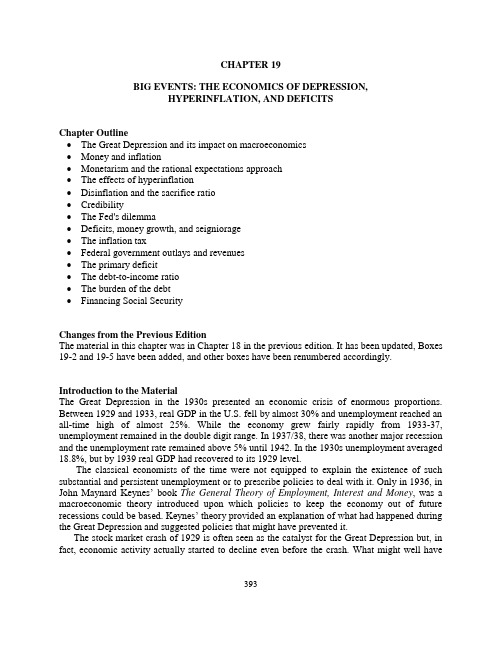
CHAPTER 19BIG EVENTS: THE ECONOMICS OF DEPRESSION,HYPERINFLATION, AND DEFICITSChapter Outline•The Great Depression and its impact on macroeconomics•Money and inflation•Monetarism and the rational expectations approach•The effects of hyperinflation•Disinflation and the sacrifice ratio•Credibility•The Fed's dilemma•Deficits, money growth, and seigniorage•The inflation tax•Federal government outlays and revenues•The primary deficit•The debt-to-income ratio•The burden of the debt•Financing Social SecurityChanges from the Previous EditionThe material in this chapter was in Chapter 18 in the previous edition. It has been updated, Boxes 19-2 and 19-5 have been added, and other boxes have been renumbered accordingly. Introduction to the MaterialThe Great Depression in the 1930s presented an economic crisis of enormous proportions. Between 1929 and 1933, real GDP in the U.S. fell by almost 30% and unemployment reached an all-time high of almost 25%. While the economy grew fairly rapidly from 1933-37, unemployment remained in the double digit range. In 1937/38, there was another major recession and the unemployment rate remained above 5% until 1942. In the 1930s unemployment averaged 18.8%, but by 1939 real GDP had recovered to its 1929 level.The classical economists of the time were not equipped to explain the existence of such substantial and persistent unemployment or to prescribe policies to deal with it. Only in 1936, in John Maynard Keynes’book The General Theory of Employment, Interest and Money, was a macroeconomic theory introduced upon which policies to keep the economy out of future recessions could be based. Keynes’ theory provided an explanation of what had happened during the Great Depression and suggested policies that might have prevented it.The stock market crash of 1929 is often seen as the catalyst for the Great Depression but, in fact, economic activity actually started to decline even before the crash. What might well have393been an average recession turned into a very severe depression due to the inept economic policies employed at the time. The Fed failed to provide needed liquidity to banks and did little to prevent the collapse of the financial system. The huge contraction in money supply due to the large numbers of bank failures caused the economic downturn. Fiscal policy was weak at best. Politicians concerned with balancing the budget raised taxes to match increases in government spending, so the decline in aggregate demand was not counteracted.Many other countries also suffered during the same period, mainly as a result of the collapse of the international financial system and the enactment of high tariffs worldwide. These policies were designed to protect domestic producers in an attempt to improve each country’s domestic trade balance at the expense of foreign trading partners. However, the attempts to "export" unemployment ultimately resulted in an overall decline in world trade and production.In the U.S., many institutional changes and administrative actions, collectively known as the New Deal, were implemented in the 1930s. The Fed was reorganized and new institutions were created, including the FDIC, the SEC, and the Social Security Administration. Public works programs and a program to establish orderly competition among firms were also implemented.The experience of the Great Depression led to the belief that the economy is inherently unstable and active stabilization policy is needed to maintain full employment. Keynes was an advocate of active government policy. In his work, he explained what had happened in the Great Depression and what could be done to avoid a recurrence. Many years later, Milton Friedman and Anna Schwartz offered a different explanation. In their book A Monetary History of the United States, Friedman and Schwartz argued that the severe decline in money supply, caused by the Fed’s failure to prevent banks from failing, was the reason for the severity of the Great Depression. They claimed that monetary policy is very powerful and that fluctuations in money supply can explain most of the fluctuations in GDP over the last century. This argument provided the impetus for new research on the effects of fiscal and monetary stabilization policies. While economists are still debating these issues, we can conclude that monetary policy can affect the behavior of output in the short and medium run, but not in the long run. In the long run, increases in the growth rate of money supply will simply lead to increases in the rate of inflation. Box 19-3 gives an overview of the monetarist positions on the importance of money for the economy, while Box 19-2 quotes Fed Chairman Ben Bernanke, who admits that the magnitude of the Great Depression was indeed the result of the Fed’s action—or, more accurately, inaction.The link between inflation and monetary growth can easily be derived from the quantity theory of money equation:MV = PY ==> %∆M + %∆V = %∆P + %∆Y ==> m + v = π + y ==> π = m - y + v In other words, the rate of inflation (%∆P = π) is determined by the difference between the growth rate of nominal money supply (%∆M = m) and the growth rate of real output (%∆Y = y), adjusted for the percentage change in the income velocity of money (%∆V = v).Figure 19-1 shows that trends in the rate of inflation and the growth of money supply (M2) have been somewhat similar over the last four decades. There is plenty of evidence to support the notion that in the long run, inflation is a monetary phenomenon here in the U.S. as well as in other countries. However, there are short-run variations, indicating that changes in velocity and output growth have also affected the inflation rate. By the mid 1990s, the relationship between394M2 growth and inflation had largely broken down, even for the long run. It is still true, however, that there has never been inflation in the long run without rapid growth of money supply, and the faster money grew the higher the rate of inflation.Although there is no exact definition, countries are said to experience hyperinflation when the inflation rate reaches 1,000% annually. Countries that have experienced hyperinflation have all had huge budget deficits which, in many cases, originated from increased government spending during wartime. A classical example is the German hyperinflation of 1922/23. In an economy experiencing hyperinflation, there is often widespread indexing, most likely to foreign exchange rates rather than to the price level, since prices are changing so fast. Eventually, hyperinflation becomes too much to bear and the government is forced to take harsh measures, including fiscal reform and the introduction of a new monetary unit pegging the new money to a foreign currency. Box 19-4 on the situation in Bolivia in the 1980s provides a good example of how hyperinflation can be stopped. It also points out that the costs are great in terms of decreasing per-capita income. In 1985, Bolivia stopped external debt service, raised taxes, reduced money creation, and stabilized the exchange rate. Inflation came down quickly, but per-capita income in 1989 was 35 percent less than it had been a decade earlier.In its fight against hyperinflation, Israel tried to keep unemployment rates low by instituting wage and price controls while also sharply cutting budget deficits and rationing credit. These measures reduced the rate of inflation significantly. In the late 1980s, the governments of Argentina and Brazil imposed wage-price controls but failed to supplement them with fiscal austerity, so the result was much less satisfactory, although they, like many South American countries eventually succeeded in lowering their inflation rates. In the early 1990s, countries in Eastern Europe experienced brief periods of high inflation during their adjustments from centrally planned economies to more market based economies (as shown in Table 19-6). There is no guarantee that periods of hyperinflation will not surface again. New Box 19-5 describes the situation in Zimbabwe where the decision made in 2006 to print more money to finance higher government spending led to inflation rates in excess of 1,000%.When inflation is high, policy makers must focus on reducing it without causing a major economic downturn. This is fairly difficult to accomplish, however, since labor contracts tend to reflect past expectations and new contract negotiations take time. In addition, it may be difficult for a central bank to gain credibility in its fight against inflation because of its behavior in the past. Credibility is important, since inflationary expectations adjust down faster if people believe that a government is serious in its attempt to reduce inflation. If this is the case, the expectations-adjusted Phillips curve shifts to the left sooner and the economy adjusts more quickly to the full-employment level of output at a lower inflation rate. But some increase in unemployment is almost always needed to reduce inflation, since real wages need to adjust down to their full-employment level. The costs to society are often measured in terms of the sacrifice ratio, that is, the ratio of the cumulative percentage loss of GDP to the achieved reduction in the inflation rate.Probably all economists now agree with the monetarist propositions that rapid money growth tends to be inflationary and inflation cannot be kept low unless money growth is kept low. We also know that monetary policy has long and variable lags. But other monetarist positions remain more controversial, including those that suggest that the economy is inherently stable and that monetary targets are better than interest rate targets. The rational expectations approach can be seen as an extension of the monetarist approach, with a strong belief that markets clear rapidly395and people use all information available to them. This is why they advocate policy rules rather than discretion and place emphasis on the credibility of policy makers. Box 19-6 highlights the rational expectations approach.Any government that is unwilling to show fiscal restraint will ultimately be faced with excessive money growth and an increase in the inflation rate. Continued large government budget deficits create a policy dilemma for a central bank, which must decide whether to monetize the debt. If the central bank decides not to finance the debt, the increased borrowing needs of the government may drive interest rates up, leading to the crowding out of private spending. The central bank may then be blamed for slowing down economic growth. But if the central bank is worried about high interest rates and monetizes the debt in order to keep interest rates low, inflation may increase with the central bank taking the blame.The financing of government spending through the creation of high-powered money is an alternative to explicit taxation. Inflation acts like a tax since the government can spend more by printing money while people can spend less, since some of their income must be used to increase their nominal money holdings. The inflation tax revenue is defined as:inflation tax revenue = (inflation rate)*(the real money base).The ability of the government to raise additional tax revenue through the creation of money (and therefore inflation) is called seigniorage, and Table 19-7 shows some empirical evidence of the inflation tax revenue raised as percentage of GDP for some Latin American countries. However, there is a limit to how much revenue a government can raise through an inflation tax. As inflation increases, people reduce their currency holdings and banks reduce their excess reserves, since holding money becomes more costly. Eventually the real monetary base falls so much that the government's inflation tax revenue decreases. Figure 19-3 shows this graphically.While higher deficits can cause higher inflation if they are financed through money creation, higher inflation may also contribute to deficits, since inflation reduces the real value of tax payments. In addition, high nominal interest rates (caused by high inflation) raise the nominal interest payments the government must make on the national debt. The inflation-adjusted deficit corrects for that and is defined in the following way:inflation-adjusted deficit = total deficit - (inflation rate)*(national debt).Large government budget deficits and rapid monetary expansion seem to be inevitable parts of hyperinflation. The high rate of monetary expansion originates in the government's desire to raise its inflation tax revenue. However, the government can only be successful if it prints money faster than the public anticipates. Eventually, the process will break down, as the real money base becomes smaller and smaller.During the 1980s, the U.S. experienced very large budget deficits, which were temporarily brought under control in the late 1990s, only to increase sharply again in 2002. Figure 19-4 shows the trend in U.S. budget deficits as percentage of GDP, while Tables 19-8 and 19-9 give an overview of trends in the U.S. government's outlays and revenues. It is interesting to note that entitlements and interest payments on the national debt have increased significantly over the last396four decades. On the revenue side, corporate income taxes as a share of GDP have declined, while social insurance taxes have increased substantially.To highlight the role of the national debt in the budget, it is useful to distinguish between the actual budget deficit and the primary (non-interest) budget deficit. The U.S. budget deficits in the 1990s were actually more a result of high interest payments on the previously incurred debt than of government spending exceeding tax revenues. This is the legacy of past deficits. As the national debt accumulates, its interest costs accelerate, contributing even more to the budget deficit. The national debt is the result of all past and present budget deficits, and the process by which the Treasury finances the debt is called debt management. As old government securities mature, the Treasury issues new securities to make the payments on old ones.Robert Eisner has argued that it is important to recognize that the government has assets and not just debts. Any spending on infrastructure should be treated as accumulation of real capital and offset by the debt issued to pay for it. In other words, just like private spending, government expenditures should be separated into government “consumption” and government “investment.”With the U.S. gross national debt now exceeding $8.5 trillion (or over $28,000 per capita), it becomes important to consider its real burden. If individuals who hold government bonds consider an increase in government debt as an increase in their personal wealth, they will consume more and a lower share of GDP will be invested. This will lead to a lower rate of capital accumulation and slower future economic growth. Another concern is that foreigners hold a large part of the debt. Since the burden of future tax payments on this part of the debt (plus interest) will fall on U.S. taxpayers while the recipients of these payments will be foreigners, there will be a reduction in U.S. net wealth.High deficits cannot be sustained indefinitely, but as long as national income is growing faster than the national debt (implying a declining debt-income ratio), the potential for instability is fairly low. In the 1990s, there was widespread sentiment that government had grown too big and that sound fiscal policy had to be implemented. The fiscal restriction finally succeeded in turning the large budget deficits of the 1980s into budget surpluses in 1998. A debate quickly began among politicians about the best ways to put the surplus to use. Was it better to cut taxes, increase spending, or gradually pay off the national debt? The path chosen by the Bush administration was a massive tax cut, leading to renewed budget deficits in 2002.Another debate revolves around Social Security reform. There is increasing concern about the financial difficulties that the Social Security system will face in the near future. The system is financed to a large extent on a pay-as-you-go basis, with most of the earmarked taxes paid by current workers being used immediately to finance the Social Security benefits of current retirees. Such a transfer of resources from the young to the old can be accomplished if:• A growing population increases the ratio of workers to retirees. If population growth slows, however, then contributions have to be increased or benefits have to be cut.•High-income growth allows retirement benefits to be higher than past contributions, since the source of the benefits is the higher income of the younger generations. If income growth slows, however, then the system may face financing difficulties.•The political situation is favorable. A larger percentage of older people than younger people vote so the elderly can enforce the intergenerational transfer through the political system. But at some point, the young, who expect to receive lower benefits than their parents relative to their contributions, may refuse to support the system through their taxes.397While the Social Security system is often seen as a “forced savings system,” which makes sure that everyone accumulates some wealth for retirement, there is strong empirical evidence that the system actually reduces national saving due to its pay-as-you-go financing. The decline in saving reduces the rate of capital accumulation, which lowers productivity and future living standards.The Social Security trust fund actually has been growing as a result of the Social Security Reform of 1983, but current predictions are that the system will be bankrupt after 2045 when most of the baby-boomer generation will have retired. While most people do not wish to see the Social Security system totally abandoned, additional reforms are very likely in the near future. The central question is how to earn higher returns on the funds invested to prevent the system from insolvency and how to preserve equity for those who have already paid into the system. Suggestions for LecturingStudents who follow the news see stock prices fluctuate daily and they probably heard about past stock market bubbles and crashes. These students will be curious about the impact of major swings in stock market activity on the economy. Most people assume that the stock market crash of October, 1929 marked the beginning of the Great Depression and are not aware that economic activity had actually begun to decline earlier. A good way to introduce the material in this chapter is to ask: “Could a Great Depression happen again?” or “Do stock market crashes cause economic downturns?” Either will lead to a lively class discussion that can help to highlight several of the issues raised in the chapter. In this discussion the major stock market crash of October, 1987 and the decline in (especially high-tech) stock values that started in March, 2000 will undoubtedly come up. They are reminders that stock market bubbles will always eventually burst and that there is considerable risk associated with buying stocks.Most economists now agree that the magnitude of the Great Depression was exacerbated by inadequate fiscal and monetary policy responses. The Fed’s failure to inject e nough liquidity into the banking system to prevent failures led to a severe contraction in the supply of money and an economic downturn, and. Policy makers also did little initially to stimulate economic activity through fiscal policy. The severity of the economic situation in the 1930’s is not surprising to economists today, as no well-developed economic theory existed at the time that could deal with a disturbance of this magnitude. It was not until John Maynard Keynes offered an explanation of what had happened during the Great Depression and suggested ways to prevent future recessions that macroeconomists began to ponder the values of fiscal and monetary stabilization policies. It is no wonder that Keynes is seen by many as the “father of all macroeconomists.”Economic theories are generally pro ducts of their time and, as mentioned above, Keynes’macroeconomic theory was developed as a result of the Great Depression. His explanation and prescription for preventing future depressions were widely accepted, but did not have much impact on policy making in the U.S. until the 1960s, when the government followed (mostly fiscal) activist policies to ensure full employment.The handling of the major stock market crash of 1987 appears to indicate that policy makers have learned from past mistakes. Stock values dropped by more than 24% in October of 1987, but we did we not see a severe downturn in economic activity. Why not? For one, Alan398Greenspan, who had been appointed as chair of the Board of Governors of the Fed only a few months earlier, was conscious of what had happened in 1929 and immediately assured financial markets that the Fed would provide the liquidity needed to prevent a financial collapse. The Fed quickly started to undertake open market purchases in an effort to drive interest rates down. In addition, as a result of institutional changes implemented after the Great Depression, government now has a much larger role in the economy. Students should be aware that the Great Depression not only shaped modern macroeconomic thinking and approaches to stabilization policy, but also shaped the structure of many U.S. institutions. Instructors may want to spend some time talking about these institutions and their importance to our economy.It also should be noted that the economy was in much better shape when the stock market crashed in 1987 than it was in 1929. While we can only speculate on what would have happened had the economy been in worse shape, the existence of programs such as Social Security and unemployment insurance would have dampened the severity of a downturn by providing some automatic stability. In addition, the existence of the FDIC, which insures all bank deposits up to $100,000, now serves to avoid panic in financial markets and runs on banks.The recession in 1981/82, which was the most severe recession since the Great Depression and brought the unemployment level close to 11%, provides another good example that policy makers now react much more swiftly to major economic upheavals. Even though the recession was fairly severe, it did not last for an extended period, since expansionary policies were implemented almost immediately after the magnitude of the downturn became clear.There are still disagreements about the primary causes for the Great Depression and these should be clarified. The Keynesian explanation concentrates on spending behavior, that is, the reduction in consumption and the collapse of investment. The decrease in aggregate demand was exacerbated by the restrictive fiscal policy implemented by the government trying to balance the budget. The monetarist explanation concentrates on the behavior of money and asserts that the Fed failed to prevent the collapse of the banking system. The large number of bank failures led to a loss of confidence in the banking system, an enormous increase in the currency-deposit ratio, and therefore a huge decrease in the money multiplier. Monetarists see the resulting severe decline in money supply as the cause of the Great Depression. Both explanations fit the facts and it is important for instructors to point out that there is no inherent conflict between them; in fact, they complement one another.While the programs of the New Deal are largely credited with revitalizing the economy in the mid-1930s, probably one of the most important factors was the sharp increase in money supply, starting in 1933. This is often a forgotten fact. It should be noted that while unemployment remained high, the deflation of prices and wages stopped after 1933, and output began to rebound. In addition, some of the programs implemented by the government after the Great Depression helped to keep wages from falling further.The fact that unemployment’s downward pressure on wages tends to weaken if high unemployment is persistent should also be mentioned at this point. The possibility that the behavior of nominal wages affects the rate of inflation should be discussed with reference to the situation in some European countries, where the unemployment rate has been above the levels experienced in the U.S. for quite some time.The German hyperinflation of 1922-23, when the inflation rate averaged 322% per month, provides another example of a major economic event that shaped macroeconomic thinking. But399students will probably prefer to discuss more recent examples, such as the Bolivian experience of the 1980s highlighted in Box 19-4 or the situation in Zimbabwe starting in 2006. Both cases make clear that the cost of stopping hyperinflation can be extremely high in terms of a decreased standard of living. The discussion should make it clear that large budget deficits and rapid monetary growth are always prevalent in times of hyperinflation, and only draconian measures can ensure a reduction in inflationary expectations. Without such measures the economy will collapse and has to be completely restructured, with the introduction of a new monetary unit that may be pegged to a foreign exchange rate.There is no exact definition of hyperinflation, but it is said to exist when the inflation rate reaches 1,000% on an annual basis. Students will always remember the following definition of inflation in general: “inflation is nothing more than too much money chasing too few goods.” But is inflation “always and everywhere a monetary phenomenon,” as Milton Friedman put it? Figure 19-1 indicates that the rate of inflation and the growth rate of M2 show somewhat similar long-run trends (at least until about 1993), but there are large variations in the short run. In other words, the link between monetary growth and the inflation rate is by no means precise. For one, growth in output affects the inflation rate and real money holdings. Interest rate changes and financial innovations also affect desired money holdings and therefore the income velocity of money. Empirical evidence indicates that the velocity of M2 has shown a fairly constant long-run trend from the 1960s to the 1990s, while the velocity of M1 has fluctuated significantly over the last few decades. Considering the enormous changes that took place in the U.S. banking system in the 1980s, it is surprising that the income velocity of M2 actually stayed as stable as it did. By the late 1990s, the link between M2 growth and the inflation rate had largely broken down; the possible causes and any monetary policy implications should be discussed.By now, students should be familiar with the quantity theory of money equation and should be able to derive the equation that shows the long-run relationship between money growth, output growth, velocity changes, and the rate of inflation. We can thus derive the following:MV = PY ==> %∆M + %∆V = %∆P + %∆Y ==> %∆P = %∆M - %∆Y + %∆V==> π = m - y + v.This equation indicates that higher growth rates of money (%∆M = m) adjusted for growth in output (%∆Y = y) and changes in velocity (%∆V = v) are associated with higher inflation rates (%∆P = π). The strict monetary growth rule is based on this equation and suggests that a zero inflation rate can be achieved if money supply is only allowed to grow at the same rate as the long-run trend of output, assuming that velocity remains stable. It should be made clear, that this equation shows only a long-run relationship and that output growth and velocity can be highly variable in the short run, causing great variations in the inflation rate.Besides looking at the role of monetary growth in determining the inflation rate, instructors may also want to spend some time looking at the role of nominal wages and labor productivity. Just by recalling the simple equationw = W/P,400。
2024年多恩布什宏观经济学ppt课件

03
货币与银行体系
CHAPTER
11
货币供给与需求理论
货币供给
指一国或一地区在一定时 期内可用于社会经济交易 的货币总量,包括现金和 存款货币。
2024/2/29
货币需求
指在一定时期内,社会各 经济主体(包括个人、企 业和政府)愿意并能够以 货币形式持有的数量。
货币供需均衡
货币供给与货币需求在一 定条件下达到相对平衡的 状态,是宏观经济稳定的 重要基础。
3
宏观经济学概述
1 2
宏观经济学定义
研究整体经济现象,包括国家经济增长、通货膨 胀、失业等问题。
宏观经济学重要性
为政策制定者提供理论支持,指导国家经济发展 。
3
宏观经济学与微观经济学关系
两者相互补充,共同构成完整经济学体系。
2024/2/29
4
多恩布什与宏观经济学
多恩布什生平简介
著名经济学家,对宏观经济学有深入研究。
通货膨胀类型与原因
包括需求拉动型通货膨胀、成本推动型通货膨胀、货币型 通货膨胀等,原因涉及总需求过度、成本上升、货币超发 等。
失业与通货膨胀的关系
菲利普斯曲线揭示了失业与通货膨胀之间存在此消彼长的 关系,但长期内二者并无必然联系。治理失业和通货膨胀 需要采取综合性的政策措施。
10
2024/2/29
学习方法建议
注重理论与实践相结合, 关注经济政策动态。
6
2024/2/29
02
国民收入与经济增长
CHAPTER
7
国民收入核算体系
国内生产总值(GDP)
一个国家或地区在一定时期内生产的所有最 终商品和服务的市场价值总和。
国民收入(NI)
Chapter_14 Investment Spending多恩布什宏观经济学(教学课件)PPT

Flow of investment is quite small compared to the stock of capital.
• Capital wears out over time must include depreciation, d • The complete formula for the rental cost of capital is:
The complete formula for trhe rcer nt ald co stio f cae pi tald is
of capital
• Diminishing marginal product of capital means that each successive unit of capital yields less than the previous unit Figure 14-2
• An increase in the rental cost of capital can only be justified by an increase in the marginal product of capital, and a lower level of K
14-4
The Desired Capital Stock
• Firms use capital, along with labor and other resources, to produce output The goal of a given firm is to maximize profits
宏观经济学(第十版)N格里高利曼昆-2024鲜版

通货膨胀的类型
根据通货膨胀的成因和特点,可以将通货膨胀分为需求拉上型通货膨胀、成本推进型通 货膨胀、输入型通货膨胀和结构性通货膨胀等类型。
2024/3/28
通货膨胀的原因
通货膨胀的原因较为复杂,可能包括总需求过度、成本上升、国际收支失衡、货币供应 过多等因素。
16
经济增长的定义、影响因素与政策
2024/3/28
货币政策的定义、目标与工具
价格稳定
通过控制通货膨胀率,保持物价稳定,避免经济波动。
经济增长
通过调节利率和信贷条件,促进投资和消费,推动经济增长。
2024/3/28
32
货币政策的定义、目标与工具
2024/3/28
• 汇率稳定:在开放经济中,通过干预外汇市场, 维护本国货币汇率的稳定。
33
货币政策的定义、目标与工具
宏观经济学(第十版 )N格里高利曼昆
2024/3/28
1
目录
2024/3/28
• 引言 • 国民收入核算与宏观经济指标 • 失业、通货膨胀与经济增长
2
目录
2024/3/28
• 货币、利率与金融市场 • 总需求与总供给模型 • 财政政策与货币政策 • 开放经济下的宏观经济政策
3
引言
01
2024/3/28
失业的类型
根据失业的原因和性质,可以将 失业分为摩擦性失业、结构性失 业、周期性失业和自然失业等类 型。
失业的原因
失业的原因多种多样,包括经济 周期波动、产业结构调整、技术 进步、劳动力市场制度不完善、 信息不对称等。
2024/3/28
15
通货膨胀的定义、类型与原因
通货膨胀的定义
通货膨胀是指一般物价水平持续上涨的现象,即货币的购买力不断下降的过程。
10宏观经济学英文版(多恩布什)课后习题答案全解

CHAPTER 10MONEY, INTEREST, AND INCOMEAnswers to Problems in the Textbook:Conceptual Problems:1. The model in Chapter 9 assumed that both the price level and the interest rate were fixed. But the IS-LM model lets the interest rate fluctuate and determines the combination of output demanded and the interest rate for a fixed price level. It should be noted that while the upward-sloping AD-curve in Chapter 9 (the [C+I+G+NX]-line in the Keynesian cross diagram) assumed that interest rates and prices were fixed, the downward-sloping AD-curve that is derived at the end of Chapter 10 from the IS-LM model lets the price level fluctuate and describes all combinations of the price level and the level of output demanded at which the goods and money sector simultaneously are in equilibrium. 2.a. If the expenditure multiplier (α) becomes larger, the increase in equilibrium income caused by a unitchange in intended spending also becomes larger. Assume investment spending increases due to a change in the interest rate. If the multiplier α becomes larger, any increase in spending will cause a larger increase in equilibrium income. This means that the IS-curve will become flatter as the size of the expenditure multiplier becomes larger.If aggregate demand becomes more sensitive to interest rates, any change in the interest rate causes the [C+I+G+NX]-line to shift up by a larger amount and, given a certain size of the expenditure multiplier α, this will increase equilibrium income by a larger amount. As a result, the IS-curve will become flatter.2.b. Monetary policy changes affect interest rates and this leads to a change in intended spending, whichis reflected in a change in income. In 2.a. it was explained that a steep IS-curve means either that the multiplier α is small or that desired spending is not very interest sensitive. Therefore, an increase in money supply will reduce interest rates. However, this does not result in a large increase in aggregate demand if spending is very interest insensitive. Similarly, if the multiplier is small, then any change in spending will not affect output significantly. Therefore, the steeper the IS-curve, the weaker the effect of monetary policy changes on equilibrium output.3. Assume that money supply is fixed. Any increase in income will increase money demand and theresulting excess demand for money will drive the interest rate up. This, in turn, will reduce the quantity of money balances demanded to bring the money sector back to equilibrium. But if money demand is very interest insensitive, then a larger increase in the interest rate is needed to reach a new equilibrium in the money sector. As a result, the LM-curve becomes steeper.Along the LM-curve, an increase in the interest rate is always associated with an increase in income. This means that an increase in money demand (due to an increase in income) has to be offset by a decrease in the quantity of money demanded (due to an increase in the interest rate) to keep the money sector in equilibrium. But if money demand becomes more income sensitive, a smaller change in income is required for any specific change in the interest rate to keep the money sector in equilibrium. Therefore, the LM-curve becomes steeper as money demand becomes more income sensitive.4.a. A horizontal LM-curve implies that the public is willing to hold whatever money is supplied at anygiven interest rate. Therefore, changes in income will not affect the equilibrium interest rate in the money sector. But if the interest rate is fixed, we are back to the analysis of the simple Keynesian model used in Chapter 9. In other words, there is no offsetting effect (or crowding-out effect) to fiscal policy.14.b. A horizontal LM-curve implies that changes in income do not affect interest rates in the money sector.Therefore, if expansionary fiscal policy is implemented, the IS-curve shifts to the right, but the level of investment spending is no longer negatively affected by rising interest rates, that is, there is no crowding-out effect. In terms of Figure 10-3, the interest rate not longer serves as the link between the goods and assets markets.4.c. A horizontal LM-curve results if the public is willing to hold whatever money balances are suppliedat a given interest rate. This situation is called the liquidity trap. Similarly, if the Fed is prepared to peg the interest rate at a certain level, then any change in income will be accompanied by an appropriate change in money supply. This will lead to continuous shifts in the LM-curve, which is equivalent to having a horizontal LM-curve, since the interest rate will never change.5. From the material presented in the text we know that when intended spending becomes more interestsensitive, then the IS-curve becomes flatter. Now assume that an increase in the interest rate stimulates saving and therefore reduces the level of consumption. This means that now not only investment spending but also consumption is negatively affected by an increase in the interest rate. In other words, the [C+I+G+NX]-line in the Keynesian cross diagram will now shift down further than previously and the level of equilibrium income will decrease more than before. In other words, the IS-curve has become flatter.This can also be shown algebraically, since we can now write the consumption function as follows:C = C* + cYD - giIn a simple model of the expenditure sector without income taxes, the equation for aggregate demand will now beAD = A o + cY - (b + g)i.From Y = AD ==> Y = [1/(1 - c)][A o - (b + g)i] ==>i = [1/(b + g)]A o - [(1 - c)/(b + g)]YTherefore, the slope of the IS-curve has been reduced from (1 - c)/b to (1 - c)/(b + g).6. In the IS-LM model, a simultaneous decline in interest rates and income can only be caused by a shiftof the IS-curve to the left. This shift in the IS-curve could have been caused by a decrease in private spending due to negative business expectations or a decline in consumer confidence. In 1991, the economy was in a recession and firms did not want to invest in new machinery and, since consumer confidence was very low, people were not expected to increase their level of spending. In the IS-LM diagram the adjustment process can be described as follows:I o↓ ==> Y ↓ (the IS-curve shifts left) ==> m d↓ ==> i ↓ ==> I ↑ ==> Y ↑. Effect: Y ↓ and i ↓ .2ii1i221Technical Problems:1.a. Each point on the IS-curve represents an equilibrium in the expenditure sector. Therefore the IS-curvecan be derived by settingY = C + I + G = (0.8)[1 - (0.25)]Y + 900 - 50i + 800 = 1,700 + (0.6)Y - 50i ==>(0.4)Y = 1,700 - 50i ==> Y = (2.5)(1,700 - 50i) ==> Y = 4,250 - 125i.1.b. The IS-curve shows all combinations of the interest rate and the level of output such that theexpenditure sector (the goods market) is in equilibrium, that is, intended spending is equal to actual output. A decrease in the interest rate stimulates investment spending, making intended spending greater than actual output. The resulting unintended inventory decrease leads firms to increase their production to the point where actual output is again equal to intended spending. This means that the IS-curve is downward sloping.1.c. Each point on the LM-curve represents an equilibrium in the money sector. Therefore the LM-curvecan be derived by setting real money supply equal to real money demand, that is,M/P = L ==> 500 = (0.25)Y - 62.5i ==> Y = 4(500 + 62.5i) ==> Y = 2,000 + 250i.1.d. The LM-curve shows all combinations of the interest rate and level of output such that the moneysector is in equilibrium, that is, the demand for real money balances is equal to the supply of real money balances. An increase in income will increase the demand for real money balances. Given a fixed real money supply, this will lead to an increase in interest rates, which will then reduce the quantity of real money balances demanded until the money market clears. In other words, the LM-curve is upward sloping.1.e. The level of income (Y) and the interest rate (i) at the equilibrium are determined by the intersectionof the IS-curve with the LM-curve. At this point, the expenditure sector and the money sector are both in equilibrium simultaneously.From IS = LM ==> 4,250 - 125i = 2,000 + 250i ==> 2,250 = 375I ==> i = 6==> Y = 4,250 - 125*6 = 4,250 - 750 ==> Y = 3,500Check: Y = 2,000 + 250*6 = 2,000 + 1,500 = 3,5003i125 ISLM62,000 3,500 4,250 Y2.a. As we have seen in 1.a., the value of the expenditure multiplier is α= 2.5. This multiplier αisderived in the same way as in Chapter 9. But now intended spending also depends on the interest rate, so we no longer have Y = αA o, but ratherY = α(A o - bi) = (1/[1 - c + ct])(A o - bi) ==> Y = (2.5)(1,700 - 50i) = 4,250 - 125i.2.b.This can be answered most easily with a numerical example. Assume that government purchasesincrease by ∆G = 300. The IS-curve shifts parallel to the right by==> ∆IS = (2.5)(300) = 750.Therefore IS': Y = 5,000 - 125iFrom IS' = LM ==> 5,000 - 125i = 2,000 + 250i ==> 375i = 3,000 ==> i = 8==> Y = 2,000 + 250*8 ==> Y = 4,000 ==> ∆Y = 500When interest rates are assumed to be constant, the size of the multiplier is equal to α = 2.5, that is, (∆Y)/(∆G) = 750/300 = 2.5. But when interest rates are allowed to vary, the size of the multiplier is reduced to α1 = (∆Y)/(∆G) = 500/300 = 1.67.2.c. Since an increase in government purchases by ∆G = 300 causes a change in the interest rate of 2percentage points, government spending has to change by ∆G = 150 to increase the interest rate by 1 percentage point.2.d. The simple multiplier α in 2.a. shows the magnitude of the horizontal shift in the IS-curve, given achange in autonomous spending by one unit. But an increase in income increases money demand and the interest rate. The increase in the interest rate crowds out some investment spending and this has a dampening effect on income. The multiplier effect in 2.b. is therefore smaller than the multiplier effect in 2.a.3.a. An increase in the income tax rate (t) will reduce the size of the expenditure multiplier (α). But as themultiplier becomes smaller, the IS-curve becomes steeper. As we can see from the equation for the IS-curve, this is not a parallel shift but rather a rotation around the vertical intercept.Y = α(A o - bi) = [1/(1 - c + ct)](A o - bi) ==> i = (1/b)A o - (α/b)Y = (1/b)A o - (1/b)[1 - c + ct]Y 3.b. If the IS-curve shifts to the left and becomes steeper, the equilibrium income level will decrease. Ahigher tax rate reduces private spending and this will lower national income.3.c. When the income tax rate is increased, the equilibrium interest rate will also decrease. The adjustmentto the new equilibrium can be expressed as follows (see graph on the next page):t up ==> C down ==> Y down ==> m d down ==> i down ==> I up ==> Y up. Effect: Y ↓ and i ↓45i 1i 2214.a. If money demand is less interest sensitive, then the LM-curve is steeper and monetary policy changesaffect equilibrium income to a larger degree. If money supply is assumed to be fixed, the adjustment to a new equilibrium in the money sector has to come solely through changes in money demand. If money demand is less interest sensitive, any increase in money supply requires a larger increase in income and a larger decrease in the interest rate in order to bring the money sector into a new equilibrium.i ii 1 i 1 2 2i 20 120 12The adjustment process in each of the two diagrams is the same; however, in the case of a more interest-sensitive money demand (a flatter LM-curve), the change in Y and i will be smaller.(M/P) up ==> i down ==> I up ==> Y up ==> m d up ==> i up Effect: Y ↑ and i ↓Section 10-5 derives the equation for the LM-curve and the equation for the monetary policy multiplier asi = (1/h)[kY - (M/P)] and (∆Y)/∆(M/P) = (b/h)γrespectively. If money demand becomes more interest sensitive, the value of h becomes larger and the slope of the LM-curve becomes flatter, while the size of the monetary policy multiplier becomes smaller.4.b. An increase in money supply drives interest rates down. This decrease in interest rates will stimulateintended spending and thus income. If money demand becomes less interest sensitive, a larger increase in income is required to bring the money sector into equilibrium. But this implies that the overall decrease in the interest rate has to be larger, given that the interest sensitivity of spending has not changed.5. The price adjustment, that is, the movement along the AD-curve, can be explained in the followingway: With nominal money supply (M) fixed, real money balances (M/P) will decrease as the price level (P) increases. There is an excess demand for money and interest rates will rise. This will lead toa decrease in investment spending and thus the level of output demanded will decrease. In otherwords, the LM-curve will shift to the left as real money balances decrease.6. In the classical case, the AS-curve is vertical. Therefore, any increase in aggregate demand due toexpansionary monetary policy will, in the long run, not lead to any increase in output but simply lead to an increase in the price level. An increase in money supply will first shift the LM-curve to the right.This implies a shift of the AD-curve to the right. Therefore we have excess demand for goods and services and prices will begin to rise. But as the price level rises, real money balances will begin to fall again, eventually returning to their original level. Therefore, the shift of the LM-curve to the right due to the expansionary monetary policy and the resulting shift of the AD-curve will be exactly offset by a shift of the LM-curve to the left and a movement along the AD-curve to the new long-run equilibrium due to the price adjustment. At this new long-run equilibrium, the level of output and interest rates will not have changed while the price level will have changed proportionally to the nominal money supply, leaving real money balances unchanged. In other words, money is neutral in the long run (the classical case).7.a. An increase in the demand for money will shift the LM-curve to the left, raising the interest rate andlowering the level of output demanded. As a result, the AD-curve will also shift to the left. In the Keynesian case, the price level is assumed to be fixed, that is, the AS-curve is horizontal. In this case, the decrease in income in the AD-AS diagram is equivalent to the decrease in income in the IS-LM diagram, since there is no price adjustment, that is, the real balance effect does not come into play. 7.b. An increase in the demand for money will shift the LM-curve to the left, raising the interest rate andlowering the level of output demanded. As a result, the AD-curve will also shift to the left. In the classical case, the level of output will not change, since the AS-curve is vertical. In this case, the shift in the AD-curve will simply be reflected in a price decrease, but the level of output will remain unchanged. The real balance effect causes the LM-curve to shift back to its original level, since the price decrease causes an increase in real money balances.Additional Problems:1. True or false? Explain your answer.“A decrease in the marginal propensity to save implies tha t the IS-curve will become steeper.”False A decrease in the marginal propensity to save (s = 1 - c) is equivalent to an increase in the marginal propensity to consume (c), which, in turn, implies an increase in the expenditure multiplier ( ). But with a larger expenditure multiplier, any increase in investment spending due to a decrease in the interest rate will lead to a larger increase in income. Therefore the IS-curve will become flatter and not steeper.2. True or false? Explain your answer.“If the c entral bank keeps the supply of money constant, then the money supply curve is vertical, which implies a vertical LM-curve.”6False. Equilibrium in the money sector implies that real money supply is equal to real money demand, that is,m s = M/P = m d(i,Y).This implies that any increase in income (Y) will increase the demand for money. To bring the money sector back into equilibrium, interest rates (i) have to rise simultaneously to bring the quantity of money demanded back to the original level (equal to the fixed supply of money). Therefore, to keep the money sector in equilibrium, an increase in income must always be associated with an increase in the interest rate and the LM-curve must be upward sloping.3. "Restrictive monetary policy reduces consumption and investment." Comment on thisstatement.A reduction in money supply raises interest rates, which will, in turn, have a negative effect on the level of investment spending. The level of consumption may also decrease as it becomes more costly to finance expenditures by borrowing money. But even if it is assumed that consumption is not affected by changes in the interest rate, consumption will still decrease since restrictive monetary policy will reduce national income and therefore private spending.4. "If government spending is increased, money demand will increase." Comment.A change in government spending directly affects the expenditure sector and therefore the IS-curve. But in an IS-LM framework, the money sector is also affected indirectly. An increase in the level of government spending will shift the IS-curve to the right, leading to an increase in income. But the increase in income will lead to an increase in money demand, so the interest rate will have to increase in order to lower the quantity of money demanded and to bring the money sector back into equilibrium. Overall no change in money demand can occur, since equilibrium in the money sector requires that m s = M/P = m d, that is, money supply has to be equal to money demand, and money supply is assumed to be fixed.5. "An increase in autonomous investment reduces the interest rate and therefore the moneysector will no longer be in equilibrium." Comment on this statement.An increase in autonomous investment shifts the IS-curve to the right. The increase in income leads to an increase in the demand for money, which means that interest rates increase. The increase in interest rates then reduces the quantity of money demanded again to bring the money market back to equilibrium.6. "A monetary expansion leaves the budget surplus unaffected." Comment on this statement. Expansionary monetary policy, that is, an increase in money supply, will lower interest rates (the LM-curve will shift to the right). Lower interest rates will lead to an increase in investment spending and the economy will therefore be stimulated. But a higher level of national income increases the government’s tax revenues and therefore the budget surplus will increase.7. "Restrictive monetary policy implies lower tax revenues and therefore to an increase in thebudget deficit." Comment on this statement.A decrease in money supply will shift the LM-curve to the left. This will lead to an increase in the interest rate, which will lead to a reduction in spending and thus national income. But as income decreases, so does income tax revenue. Therefore, the budget deficit will increase because of the change in its cyclical component.78. “If the demand for money becomes more sensitive to changes in income, then the LM-curvebecome s flatter.” Comment on this statement.Along the LM-curve, an increase in the interest rate is always associated with an increase in income. This means that an increase in money demand (due to an increase in income) has to be offset by a decrease in the quantity of money demanded (due to an increase in the interest rate) to keep the money sector in equilibrium. But if money demand becomes more income sensitive, a smaller change in income is required for any specific change in the interest rate to keep the money sector in equilibrium. Therefore, the LM-curve becomes steeper (and not flatter) as money demand becomes more sensitive to changes in income.9. “A decrease in the income tax rate will increase the demand for money, shifting the LM-curveto the righ t.” Comment on this statement.A decrease in the income tax rate (t) will increase the expenditure multiplier (α). But with a larger expenditure multiplier, any increase in investment spending due to a decrease in the interest rate will lead to a larger increase in income. Since fiscal policy affects the expenditure sector, the IS-curve (not the LM-curve) will shift. The IS-curve will become flatter and shift to the right. This will lead to a new equilibrium at a higher level of income (Y) and a higher interest rate (i). But money supply is fixed and the LM-curve remains unaffected by fiscal policy. Therefore, at the new equilibrium (the intersection of the new IS-curve with the old LM-curve) the demand for money will not have changed, since the money sector has to be in an equilibrium at m s = m d(i,Y).10. “If the demand for money becomes more insensitive to changes in the interest rate, equilibriumin the money sector will have to be restored mostly through changes in income. This implies a flat LM-curve.” Comment on this statement.Any increase in income will increase money demand and this will drive the interest rate up. Therefore, the quantity of money balances demanded will decline again until the money sector is back in equilibrium. But if money demand is very interest insensitive, then a larger increase in the interest rate is needed to reach a new equilibrium in the money sector. This means that the LM-curve is steep and not flat.11. Assume the following IS-LM model:Expenditure Sector Money SectorSp = C + I + G + NX M = 700C = 100 + (4/5)YD P = 2YD = Y - TA m d = (1/3)Y + 200 - 10iTA = (1/4)YI = 300 - 20iG = 120NX = -20(a) Derive the equilibrium values of consumption (C) and money demand (m d).(b) How much of investment (I) will be crowded out if the government increases its purchasesby ∆G = 160 and nominal money supply (M) remains unchanged?(c) By how much will the equilibrium level of income (Y) and the interest rate (i) change, ifnominal money supply is also increased to M' = 1,100?a. Sp = 100 + (4/5)[Y - (1/4)Y] + 300 - 20i + 120 - 20 = 500 + (4/5)(3/4)Y – 20i = 500 + (3/5)Y - 20iFrom Y = Sp ==> Y = 500 + (3/5)Y - 20i ==> (2/5)Y = 500 - 20i==> Y = (2.5)(500 - 20i) ==> Y = 1,250 - 50i IS-curveFrom M/P = m d ==> 700/2 = (1/3)Y + 200 - 10i ==> (1/3)Y = 150 + 10i==> Y = 3(150 + 10i) ==> Y = 450 + 30i LM-curve89IS = LM ==> 1,250 - 50i = 450 + 30i ==> 800 = 80i ==> i = 10==> Y = 1,250 - 50*10 ==> Y = 750C = 100 + (4/5)(3/4)750 = 100 + (3/5)750 ==> C = 550m s = M/P = 700/2 = 350 = m dCheck: m d = (1/3)750 + 200 - 10*10 = 350i25 IS o LM o10450 750 1,250 Yb. ∆IS = (2.5)160 = 400 ==> IS' = 1,650 - 50iIS' = LM ==> 1,650 - 50i = 450 + 30i ==> 1,200 = 80i ==> i = 15==> Y = 1,650 - 50*15 ==> Y = 900Since ∆i = + 5 ==> ∆I = - 20*5 ==> ∆I = - 100Check: ∆ 331510450 750 900 1,250 1,650 Yc. From M'/P = m d ==> 1,100/2 = (1/3)Y + 200 - 20i==> (1/3)Y = 350 - 20i ==> Y = 3(350 - 20i) ==> Y = 1,050 + 30iIS 1 = LM 1 ==> 1,650 - 50i = 1,050 + 30i ==> 600 = 80i ==> i = 7.5==> Y = 1,650 - 50(7.5) = 1,275.==> ∆i = - 7.5 and ∆Y = 375 as compared to (b).i1107.512. Assume the money sector can be described by these equations: M/P = 400 and m d = (1/4)Y - 10i.In the expenditure sector only investment spending (I) is affected by the interest rate (i), and the equation of the IS-curve is: Y = 2,000 - 40i.(a) If the size of the expenditure multiplier is α= 2, show the effect of an increase ingovernment purchases by ∆G = 200 on income and the interest rate.(b) Can you determine how much of investment is crowded out as a result of this increase ingovernment spending?(c)If the money demand equation were changed to m d = (1/4)Y, how would your answers in (a)and (b) change?a. From M/P = m d ==> 400 = (1/4)Y - 10i ==> Y = 1,600 + 40i LM-curveFrom IS = LM ==> 2,000 - 40i = 1,600 + 40i ==> 80i = 400 ==> i = 5==> Y = 2,000 - 40*5 ==> Y = 1,800∆IS = 2*200 = 400 ==> IS' = 2,400 - 40iIS' = LM ==> 2,400 - 40i = 1,600 + 40i ==> 80i = 800 ==> i = 10==> Y = 1,600 + 40*10 ==> Y = 2,000Therefore ∆i = + 5 and ∆Y = + 200b.Since the size of the expenditure multiplier is α = 2 but income only goes up by αY = 200, the fiscalpolicy multiplier in the IS-LM model is α1= 1. But this means that the level of investment has been reduced by 100, that is, ∆I = -100. This can be seen by restating the IS-curve as follows:Y = 2,000 - 40i = Y = 2(1,000 - 20i)Since government purchases are changed by ∆G = 200 ==> Y = 2(1,200 - 20i), which means that the IS-curve shifts by ∆IS = 2*200 = 400. But the increase in income is actually only ∆Y = 200. This implies that investment changes by ∆I = -100. Investment is of the form I = I o– 20i; however, since the interest rate went up by ∆i = 5, investment changes by ∆I = - 20*5 = - 100.From ∆Y = α(∆Sp) ==> 200 = 2(∆Sp) ==> ∆Sp = 100But since ∆Sp =∆ G + ∆I ==> 100 = 200 + ∆I ==> ∆I = - 100c. If m d= (1/4)Y, then we have the classical case, that is, a vertical LM-curve. In this case, fiscalexpansion will not change income at all. This occurs since the increase in G will be offset by a decrease in I of equal magnitude due to an increase in the interest rate.(M/P) = m d ==> 400 = (1/4)Y ==> Y = 1,600 LM-curveIS = LM ==> 2,000 - 40i = 1,600 ==> 40i = 400 ==> i = 10 ==> Y = 1,600IS' = LM ==> 2,400 - 40i = 1,600 ==> 40i = 800==> i = 20 ==> Y = 1,600 ==> ∆I = - 2001013. Assume money demand (md) and money supply (ms) are defined as: md = (1/4)Y + 400 - 15iand ms = 600, and intended spending is of the form: Sp = C + I + G + NX = 400 + (3/4)Y - 10i.Calculate the equilibrium levels of Y and i, and indicate by how much the Fed would have to change money supply to keep interest rates constant if the government increased its spending by ∆G = 50. Show your solutions graphically and mathematically.ms = md ==> 600 = (1/4)Y + 400 - 15i ==> (1/4)Y = 200 + 15i==> Y = 4(200 + 15i) ==> Y = 800 + 60i LM-curveY = C + I + G + NX ==> Y = 400 + (3/4)Y - 10i ==>(1/4)Y = 400 - 10i ==> Y = 4(400 - 10i) ==> Y = 1,600 - 40i IS-curveFrom IS = LM ==> 1,600 - 40i = 800 + 60i ==> 100i = 800 ==> i = 8 ==> Y = 1,280If government spending is increased by ∆G = 50, the IS-curve will shift to the right) by (∆IS) = 4*50 = 200. If the Fed wants to keep the interest rate constant, money supply has to be increased in a way that shifts the LM-curve to the right by exactly the same amount as the IS-curve, that is, (∆LM) = 200.From Y = 2(200 + 15i) ==> (∆Y) = 2(∆ms) ==> 200 = 2(∆ms)==> (∆ms) = 100, so money supply has to be increased by 100.Check: IS' = LM": 1,800 - 40i = 1,000 + 60i ==> 800 = 100i4018800 1000 1280 1480 1600 1800 Y14. Assume the equation for the IS-curve is Y = 1,200 – 40i, and the equation for the LM-curve isY = 400 + 40i.(a) Determine the equilibrium value of Y and i.(b) If this is a simple model without income taxes, by how much will these values change if thegovernment increases its expenditures by ∆G = 400, financed by an equal increase in lump sum taxes (∆TA o = 400)?a. From IS = LM ==> 1,200 - 40i = 400 + 40i ==>800 = 80i ==> i = 10 ==> Y = 400 + 40*10 ==> Y = 800b. According to the balanced budget theorem, the IS-curve will shift horizontally by the increase ingovernment purchases, that is, ∆IS = ∆G = ∆TA o = 400.Thus the new IS-curve is of the form: Y = 1,600 - 40i.From IS' = LM ==> 1,600 - 40i = 400 + 40i ==>1,200 = 80i ==> i = 15 ==> Y = 400 + 40*15 ==> Y = 1,00015. Assume you have the following information about a macro model:Expenditure sector: Money sector:11。
湘潭大学宏观经济学课件(多恩布什第十版)-第3章修改版+第四章

0.08
0.10
0.06
0.08
0.04
0.06 0 100 200 300 400
0.02 0 2000 4000 6000
数据来源:《新中国50年统计资料汇编》和作者的计算
经济增长所要解决的核心问题
经济增长的引擎是什么? 为什么经济体间存在收入差距?
贫穷经济体能否以及如何赶超富裕的经 济体?
稳态中的产出增长率是外生的, 在这种情况下它等于人口增长率n ,因而独立于储蓄率s 虽然储蓄率增加不影响稳态增长 率,但是可以提高稳态增长水平
新古典经济增长模型重要结论
若允许生产率增长,并存在稳态 增长率的话,可得出稳态增长率 仍是外生的。稳态的人均收入增 长率由技术进步率决定。总产出 的稳态增长率是n+g
注数据来自Jones(1998),第42页;资本、劳动的收入份额是1/3:2/3。
索罗剩余
⊿Y/Y=[(1-θ)* ⊿N/N]+[θ*⊿K/K]+⊿A/A
⊿A/A= ⊿Y/Y-[(1-θ)* ⊿N/N]+[θ* ⊿K/K]
A的变化解释了所有非源于要Байду номын сангаас投入 变化的生产率变化的,可以衡量技术进 步
人均产出增长的核算
二、新古典模型的基本公式
2、基本公式的意义
▲资本存量的决定因素 ▲人均资本存量的变动量= 人均储蓄量-人均维持原装备水平所 需资本
三、稳态均衡分析
1、稳态均衡的含义 ▲经济处于长期均衡状态 ▲人均经济变量保持不变 ∆y=∆k=0 ▲经济总量按照人口增长率n增加 ∆ Y/Y= ∆ K/K= ∆ N/N=n
1000
2.3 经济增长的典型事实之三
对外经济贸易大学金融学院金融组织学(金融风险管理)考博真题-参考书-分数线-复习方法-育明考博

对外经济贸易大学金融学院金融组织学(金融风险管理)考博指导与分析一、对外经济贸易大学金融学院考博资讯从2014年开始,除专职教师和专职科研人员外对外经济贸易大学不在招收以在职方式攻读的博士研究生,仅招收全日制脱产博士研究生,所有被录取的考生均须将档案迁入对外经济贸易大学管理。
本年度国际经济研究院拟录博士研究生5名,专业目录中各招生专业各方向所列招生人数均为初步意向人数,具体招生人数将根据生源状况确定,此数据仅供参考。
考试科目中,英语包括基础英语(占50%)和宏、微观经济学专业英语(占50%);经济学基础包括中级宏、微观经济学(占70%)和数学(微积分和线性代数)(占30%)。
面试中现代金融理论的前沿问题(占60%),前期研究成果(占40%)。
(一)考试科目及各方向导师:1.020204 金融学研究方向01:金融组织学(金融风险管理)。
导师是刘亚。
考试的科目:(1)1101英语(100%)。
(2)2201经济学基础(100%)。
(3)3321金融理论(100%)。
(二)复试须知1.复试方案:(1)坚持标准统一、程序公开、择优录取、宁缺毋滥的原则;(2)实行差额复试,按130%-150%的比例进行差额复试;总成绩=初试分数(满分300分)+专家组面试(满分100分)+导师对考生评价(满分100分)含专业素质40分,综合评价60分;专家组面试和导师对考生评价及格分均为60分。
(3)按总绩从高分到低分确定拟录取名单,报学校研究生招生领导小组审批。
2.复试内容:(1)所报研究方向的理论和实务;(2)英语问答,内容包括外语听力水平和口语水平测试;(3)前期科研成果,专业课和学术潜力。
3.考核方法:(1)考生介绍个人学习和工作情况,攻读博士期间的学术研究构想,时间不超过5 分钟;(2)考官根据考生的陈述提问,考生即问即答,时间不超过所5 分钟; (3)英语问答。
提问内容以学习和研究经历、某些相关的理论问题为主,时间不超过5分钟;(4)检查前期科研成果(包括公开发表的学术论文原件,国家级科研课题项目立项书,省部级纵向科研课题立项书)。
多恩布什《宏观经济学》(第10版)【教材精讲+考研真题解析】讲义与课程【39小时】
目 录第一部分 开篇导读及本书点评[1小时高清视频讲解]一、开篇导读二、本书点评及总结(结束语)第二部分 辅导讲义[31小时高清视频讲解]第1篇 导论与国民收入核算[视频讲解]第1章 导 论1.1 本章要点1.2 重难点解读第2章 国民收入核算2.1 本章要点2.2 重难点解读第2篇 增长、总供给与总需求,以及政策[视频讲解]第3章 增长与积累3.1 本章要点3.2 重难点解读第4章 增长与政策4.1 本章要点4.2 重难点解读第5章 总供给与总需求5.1 本章要点5.2 重难点解读第6章 总供给:工资、价格与失业6.1 本章要点6.2 重难点解读第7章 通货膨胀与失业的解剖7.1 本章要点7.2 重难点解读第8章 政策预览8.1 本章要点8.2 重难点解读第3篇 首要的几个模型[视频讲解]第9章 收入与支出9.1 本章要点9.2 重难点解读第10章 货币、利息与收入10.1 本章要点10.2 重难点解读第11章 货币政策与财政政策11.1 本章要点11.2 重难点解读第12章 国际联系12.1 本章要点12.2 重难点解读第4篇 行为的基础[视频讲解]第13章 消费与储蓄13.1 本章要点13.2 重难点解读第14章 投资支出14.1 本章要点14.2 重难点解读第15章 货币需求15.1 本章要点15.2 重难点解读第16章 联邦储备、货币与信用16.1 本章要点16.2 重难点解读第17章 政 策17.1 本章要点17.2 重难点解读第18章 金融市场与资产价格18.1 本章要点18.2 重难点解读第5篇 重大事件、国际调整和前沿课题[视频讲解]第19章 重大事件:萧条经济学、恶性通货膨胀和赤字19.1 本章要点19.2 重难点解读第20章 国际调整与相互依存20.1 本章要点20.2 重难点解读第21章 前沿课题21.1 本章要点21.2 重难点解读第三部分 名校考研真题名师精讲及点评[8小时高清视频讲解]一、名词解释二、简答题三、计算题四、论述题第一部分 开篇导读及本书点评[1小时高清视频讲解]一、开篇导读[0.5小时高清视频讲解]主讲老师:郑炳一、教材及教辅、课程、题库简介► 教材:多恩布什《宏观经济学》(第10版)(多恩布什、费希尔、斯塔兹著,王志伟译,中国人民大学出版社)► 教辅(两本,文库考研网主编,中国石化出版社出版)√网授精讲班【教材精讲+考研真题串讲】精讲教材章节内容,穿插经典考研真题,分析各章考点、重点和难点。
2024版年度多恩布什《宏观经济学》本科生课件

CHAPTER宏观经济学定义与研究对象宏观经济学定义宏观经济学是研究整体经济现象,包括国民经济总量、总需求与总供给、经济增长、通货膨胀、失业等问题的经济学分支。
研究对象宏观经济学主要关注整体经济运行情况,如国民生产总值(GDP)、失业率、通货膨胀率、利率、汇率等总量指标。
宏观经济学发展历程及主要流派发展历程宏观经济学起源于20世纪30年代的凯恩斯主义,随后经历了货币主义、新古典主义、新凯恩斯主义等发展阶段。
主要流派包括凯恩斯主义、货币主义、供给学派、新古典宏观经济学、新凯恩斯主义等。
各流派在理论假设、政策主张等方面存在差异。
宏观经济学与微观经济学关系相互联系宏观经济学与微观经济学是经济学的两个重要分支,二者相互联系、相互补充。
微观经济学是宏观经济学的基础,宏观经济学是微观经济学的延伸。
区别微观经济学研究个体经济单位(如家庭、企业)的经济行为,而宏观经济学研究整体经济现象;微观经济学强调市场供求均衡,宏观经济学强调国民经济总量均衡。
学习宏观经济学意义和方法学习意义学习宏观经济学有助于了解整体经济运行规律,为政府制定经济政策提供理论依据;同时,也有助于培养个人经济素养,提高分析和解决经济问题的能力。
学习方法学习宏观经济学需要掌握基本概念、原理和方法,注重理论与实践相结合;同时,也需要关注经济政策动态,了解国内外经济形势。
CHAPTER国民收入核算体系介绍国民收入定义及核算方法01国内一定时期内所有居民获得的最终产品和劳务的价值总和,包括国内生产总值(GDP)和国民生产总值(GNP)等核算方法。
国民收入核算体系构成02包括初次分配和再分配两个过程,涉及生产、分配、交换和消费四个环节。
国民收入核算体系的意义03反映一个国家或地区一定时期内的经济总量和经济发展水平,为政府制定经济政策和企业决策提供依据。
介绍哈罗德-多马模型、新古典增长模型、内生增长模型等经济增长理论,分析经济增长的源泉和动力。
经济增长理论概述包括财政政策、货币政策、产业政策、科技创新政策等,分析不同政策对经济增长的影响和效果。
Chapter_02National Income Accounting(宏观经济学,多恩布什,第十版)

From GDP to National Income
•
Use the terms output and income interchangeably in macroeconomics, but are they really equivalent?
•
There are a few crucial distinctions between them:
2-1
Chapter 2
National Income Accounting
• • • • Item Item Item Etc.
McGraw-Hill/Irwin Macroeconomics, 10e
© 2008 The McGraw-Hill Companies, Inc., All Rights Reserved. 2-2
• •
•
Ex. Social security, unemployment benefits Transfer payments are NOT included in GDP since not a part of current production Government expenditure = transfers + purchases
•
NX can be >, <, or = 0
•
2-10
Some Identities: A Simple Economy
•
• •
•
Assume national income equals GDP, and thus use terms income and output interchangeably (convenience) Begin with a simple economy: closed economy with no public sector output expressed as Y C I (4) Only two things can do with income: consume and save national income expressed as Y C S (5), where S is private savings I Y C S (6) Combine (4) and (5): C
中级宏观经济学教学大纲

《中级宏观经济学》教学大纲执笔人:何建春课程教学目的与要求:本课程是属于宏观经济的中级课程,主要面向本科专业高年级学生,要求选修的学生具有一定的经济学和经济数学基础。
通过本课程的学习,可以更好地理解和掌握现代宏观经济学的基本理论及研究方法,并用于观察、分析和解释宏观经济现象。
本课程在初级宏观经济学的基础上,着重介绍经济增长理论、开放宏观经济模型、宏观经济政策及制定,以及现代宏观经济学的微观基础。
一、教学内容与课时安排1.导论(3课时)1.1 宏观经济学的研究对象1.2 经济学家是如何思考的1.3 宏观经济学的数据2. 国民收入:源自何处,去向何方(3课时)2.1 社会总产出的决定因素2.2 国民收入的分配(要素价格的决定)2.3 产品与服务市场的均衡3. 货币与通货膨胀(3课时)3.1 货币数量论3.2 货币铸造税3.3 通货膨胀与利率3.4 名义利率与货币需求3.5 通货膨胀的社会成本4. 开放经济(3课时)4.1 资本和产品的国际流动4.2 小型开放经济中的储蓄与投资4.3 汇率5. 经济增长理论:超长期中的经济(6课时)5.1 经济增长:资本积累与人口增长5.2 经济增长:技术、经验和政策5.3 超越索洛模型:内生增长理论6. 经济波动导论(3课时)6.1 关于经济周期的事实6.2 对IS—LM模型的回顾6.3 稳定化政策7. 蒙代尔—弗莱明模型与汇率(6课时)7.1 蒙代尔—弗莱明模型7.2 浮动汇率下的小型开放经济7.3 固定汇率下的小型开放经济7.4 汇率应该浮动还是固定?7.5 价格水平变动的蒙代尔—弗莱明模型8. 总供给:通货膨胀与失业之间的短期权衡(3课时)8.1 总供给的基本理论8.2 通货膨胀、失业和菲利普斯曲线8.3 菲利普斯曲线的变异9. 总供给和总需求的动态模型(3课时)9.1 模型的要素9.2 模型的求解9.3 基本结论及政策建议10. 稳定化政策(3课时)10.1 经济政策应该对经济稳定发挥什么样的作用10.2 经济政策制定的规则:按规则实施还是相机抉择10.3 结论:在一个不确定的世界中制定政策11 政府债务与预算赤字(3课时)11.1 政策债务的规模与衡量11.2 传统的政府债务的观点11.3 李嘉图学派的政府债务的观点11.4 其他学派关于政府债务的观点12 宏观经济学的微观基础(6课时)12.1 消费理论12.2 投资理论12.3 货币供给、货币需求与银行体系13 总复习与答疑(3课时)二、教材与参考资料(一)教材曼昆:宏观经济学(第七版),中国人民大学出版社,2012中文版(二)参考资料1.布兰查德:宏观经济学(第四版)清华大学出版社,2011中文版2.多恩布什等:宏观经济学(第十版),中国人民大学出版社3.巴罗:宏观经济学:现代观点,格致出版社,2008中文版4.萨克斯:全球视角的宏观经济学,上海三联书店,1997中文版5.霍华德:现代宏观经济学:起源、发展与现状,凤凰传媒出版社,2009中文版三、考试与成绩评定本课程采用闭卷考试,其中卷面成绩占80%,平时成绩占20%。
多恩布什宏观经济学

Copyright 2007 Business School of Xiangtan University
32
Business Cycle
Copyright 2007 Business School of Xiangtan University
结论2:高通货膨胀率总是由总需求的变化 引起的。
高通货膨胀率的唯一原因是滥发货币
Copyright 2007 Business School of Xiangtan University
22
短期模型:产出波动
短期模型关注的是实际产出、失业等宏观 经济变量的波动;
短期通常假设生产要素大量闲置,产出具 有充分弹性,因此短期总供给曲线是水平 的;
那么到达3.2% 为什么会有增长?各国增长差异的原因是
什么?什么政策可提高一国长期平均增长 率?
Copyright 2007 Business School of Xiangtan University
31
经济周期与 GDP
经济周期描述的是一国经济围绕增长趋势 线进展有规律的扩张〔复苏〕与收缩〔衰 退〕的现象。
间增长率的差异 经济增长的主要原因有 新技术的开展 物质与人力资本的积累 良好的根底设施 高国内储蓄率
Copyright 2007 Business School of Xiangtan University
18
长期模型:生产能力不变的经济
决定通货膨胀率的因素是什么? 长期中,所有要素被假设处于充分就业状
背景 现实背景 理论背景 凯恩斯革命:?就业、利息和货币通论?
,1936年出版,被认为是第一部系统 地运用了总量分析方法来研究整个国民 经济活动的宏观经济学著作。
(完整版)多恩布什宏观经济学第十版课后答案
宏观经济学第二章概念题1.如果政府雇用失业工人,他们曾领取TR美元的失业救济金,现在他们作为政府雇员支取TR美元,不做任何工作,GDP会发生什么情况?请解释。
答:国内生产总值指一个国家(地区)领土范围,本国(地区)居民和外国居民在一定时期内所生产和提供的最终使用的产品和劳务的价值。
用支出法计算的国内生产总值等于消费C、投资I、政府支出G和净出口NX之和。
从支出法核算角度看:C、I、NX保持不变,由于转移支付TR美元变成了政府对劳务的购买即政府支出增加,使得G增加了TR美元,GDP会由于G的增加而增加。
2.GDP和GNP有什么区别?用于计算收入/产量是否一个比另一个更好呢?为什么?答:(1)GNP和GDP的区别GNP指在一定时期内一国或地区的国民所拥有的生产要素所生产的全部最终产品(物品和劳务)的市场价值的总和。
它是本国国民生产的最终产品市场价值的总和,是一个国民概念,即无论劳动力和其他生产要素处于国内还是国外,只要本国国民生产的产品和劳务的价值都记入国民生产总值。
GDP指一定时期内一国或地区所拥有的生产要素所生产的全部最终产品(物品和劳务)的市场价值的总和。
它是一国范围内生产的最终产品,是一个地域概念。
两者的区别:在经济封闭的国家或地区,国民生产总值等于国内生产总值;在经济开放的国家或地区,国民生产总值等于国内生产总值加上国外净要素收入。
两者的关系可以表示为:GNP=GDP+[本国生产要素在其他国家获得的收入(投资利润、劳务收入)-外国生产要素从本国获得的收入]。
(2)使用GDP比使用GNP用于计量产出会更好一些,原因如下:1)从精确度角度看,GDP的精确度高;2)GDP衡量综合国力时,比GNP好;3)相对于GNP而言,GDP是对经济中就业潜力的一个较好的衡量指标。
由于美国经济中GDP和GNP的差异非常小,所以在分析美国经济时,使用这两种的任何一个指标,造成的差异都不会大。
但对于其他有些国家的经济来说明,这个差别是相当大的,因此,使用GDP作为衡量指标会更好。
2024版宏观经济学多恩布什第十版ppt课件

2024/1/28
10
03
失业、通货膨胀与货币政 策
2024/1/28
11
失业类型、原因及影响分析
摩擦性失业
由于劳动力市场供需不匹配造成的短期失业。
结构性失业
由于经济结构变化导致某些行业或地区就业机会减少的长期失业。
2024/1/28
12
失业类型、原因及影响分析
• 周期性失业:与经济周期波动相关的失业, 通常在经济衰退时上升,经济复苏时下降。
国际贸易实践
分析国际贸易的现状、趋势和问题,如贸易保护主义、贸易摩擦 等。
36
国际金融市场运行规律和风险防范
国际金融市场概述
介绍国际金融市场的构成、功能和运行规律。
国际金融风险
分析汇率风险、信用风险、流动性风险等国际金融风险的来源和影 响。
风险防范与管理
探讨国际金融风险防范和管理的策略和方法,如风险识别、评估和控 制。
2024/1/28
4
宏观经济学研究方法与工具
2024/1/28
研究方法
宏观经济学采用实证分析和规范分析 相结合的方法,既研究经济现象“是 什么”的问题,也探讨经济运行“应 该是什么”的问题。
研究工具
宏观经济学运用大量的经济模型、图 表和数学公式等分析工具,来研究和 分析宏观经济现象及其运行规律。
5
技术进步是提高生产率和经济 增长的重要途径。通过加强科 技创新、促进科技成果转化、 培养高素质人才等方式,可以 推动技术进步和经济增长。
制度创新是经济增长的重要保 障。通过深化经济体制改革、 完善市场体系、加强法治建设 等方式,可以推动制度创新和 经济增长。
26
经济发展战略和政策选择
2024/1/28
- 1、下载文档前请自行甄别文档内容的完整性,平台不提供额外的编辑、内容补充、找答案等附加服务。
- 2、"仅部分预览"的文档,不可在线预览部分如存在完整性等问题,可反馈申请退款(可完整预览的文档不适用该条件!)。
- 3、如文档侵犯您的权益,请联系客服反馈,我们会尽快为您处理(人工客服工作时间:9:00-18:30)。
The marginal product of capital is the increase in output produced by using 1 more unit of capital in production. The rental (user) cost of capital is the cost of using 1 more unit of capital in production.
14-4
The Desired Capital Stock
•
Firms use capital, along with labor and other resources, to produce output The goal of a given firm is to maximize profits
14-3
Introduction
•
The theory of investment is the theory of the demand for capital
•
Investment is the flow of spending that adds to the stock of capital
• • •
•
Capital at the end of last period is K-1 The gap between actual and desired capital stock is (K*-K-1) A firm plans to add a fraction of the gap to last periods stock Actual capital stock at the end of the current period is then
K 0 K 1 ( K K 1 )
*
(2)
14-9
Capital Stock Adjustment
•
To increase the capital stock from K-1 to K0, the firm must achieve net investment of
I ( K 0 K 1 )
•
The general relationship among the desired capital stock, K*, rc, and output is
K g ( rc , Y )
*
(1)
14-7
From Desired Capital Stock to Investment
•
Figure 14-4 illustrates an increase in the demand for capital stock as a rightward shift in the demand for capital schedule
*
[Insert Figure 14-5 here]
( K 1 ( K K 1 )) K 1 ( K K 1 )
*
(3)
•
Figure 14-5 illustrates how the capital stock adjusts from an initial level of K-1 to the desired level K*
•
14-6
The Desired Stock of Capital
•
Firms add capital until the marginal return of the last unit added drops to the rental cost of capital
•
[Insert Figure 14-2 here]
When
deciding the optimal level of capital, firms must balance the contribution that more capital makes to their revenues against the cost of acquiring additional capital
14-5
The Desired Capital Stock
•
To derive the rental cost of capital:
•
•
firms finance the purchase of capital by borrowing over time, at an interest rate of i In the presence of inflation, the nominal dollar value of capital rises over time
• •
Upper panel shows the stock of capital Lower panel shows the corresponding level of I
14-10
Capital Stock Adjustment
•
To increase the capital stock from K-1 to K0, the firm must achieve net investment of
•
Both GDP and investment are flow variables
•
Capital is the dollar value of all the buildings, machines, and inventories at a given point in time stock value
Introduction
•
Investment:
[Insert Figure 14-1 here]
Links the present to the future Links the goods and money markets Drives much of the business cycle
•
[Insert Figure 14-4 here]
•
•
At the initial level of capital, K0, the price of capital is just high enough to generate enough investment, I0, to replace the depreciating capital In the LR, supply of new capital is very elastic, so the increase in demand is met without much change in price In the SR, price rises to P1, increasing investment flow to I1
I ( K 0 K 1 ) ( K 1 ( K K 1 )) K 1
*
[Insert Figure 14-5 here]
( K K 1 )
*(3)•Fra bibliotekEquation (3) shows investment spending as a function of K* and K-1
•
•
In this chapter we study how investment depends on interest rates and income Figure 14-1 illustrates the volatility of investment by comparing investment and GDP
14-8
Capital Stock Adjustment
•
The flexible accelerator model can be used to explain the speed at which firms plan to adjust their capital stock
Basic
•
Real cost of capital = nominal interest rate - nominal capital gain
•
At the time the firm makes an investment, the nominal interest rate is known, but the inflation rate for the coming year is not
•
Diminishing marginal product of capital means that each successive unit of capital yields less than the previous unit Figure 14-2 An increase in the rental cost of capital can only be justified by an increase in the marginal product of capital, and a lower level of K
notion: the larger the gap between the existing capital stock and the desired capital stock, the more rapid a firm’s rate of investment Firms plan to close a fraction, , of the gap between the actual and desired capital stocks each period
•
•
Any factor that increases K*, increases the rate of investment Investment contains aspects of dynamic behavior