2007_Combining rough sets and GIS techniques to assess aquifer vulnerability

合集下载

证据理论与熵值融合的知识约简新方法

证据理论与熵值融合的知识约简新方法吴根秀;吴恒;黄涛【摘要】求解决策表的最小约简已被证明是NP-hard问题，在粗糙集和证据理论的基础上提出了一种知识约简的启发式算法。

利用粗糙集等价划分的概念给出属性的信息熵，定义每个属性的熵值重要性并由此确定知识的核。

引入二分mass函数对每个属性建立一个证据函数，证据融合得到每个属性的证据重要性。

以核为起点，以证据重要性为启发，依次加入属性直至满足约简条件。

实例表明，该方法能够快速找到核和相对约简，并且该约简运用到分类上正确率也是较高的。

%It is proved that solving the minimal reduction of decision table is a NP-hard problem. This paper puts on a heuristic algorithm based on rough set and evidence theory. It gives attribute information entropy by using the concept of equivalence partitioning of rough set, and defines the attribute importance to get the core of the knowledge. It establishes an evidence function for each attribute by the concept of dichotomous mass functions, combining which to get the evi-dence importance of each attribute. Setthe core as the start of the algorithm and make size of attributes importance as heu-ristic information until it meets the reduction condition. Examples show that it can find the core and reduction quickly, and the reduction used in classification accuracy is higher.【期刊名称】《计算机工程与应用》【年(卷),期】2016(052)019【总页数】4页(P167-170)【关键词】粗糙集;知识约简;二分mass函数;熵;属性重要性【作者】吴根秀;吴恒;黄涛【作者单位】江西师范大学数学与信息科学学院，南昌 330022;江西师范大学数学与信息科学学院，南昌 330022;江西师范大学数学与信息科学学院，南昌330022【正文语种】中文【中图分类】TP31WU Genxiu，WU Heng，HUANG Tao.Computer Engineering and Applications，2016，52（19）：167-170. Rough Set［1］是波兰数学家Pawlak于1982年提出的，该理论是一种处理不精确、不完全与不相容知识的数学方法。

Effects of twin tunnels construction beneath existing shield-driven twin tunnels

Effects of twin tunnels construction beneath existing shield-driven twintunnelsQian Fang a ,⇑,Dingli Zhang a ,QianQian Li a ,Louis Ngai Yuen Wong ba School of Civil Engineering,Beijing Jiaotong University,Beijing 100044,ChinabSchool of Civil and Environmental Engineering,Nanyang Technological University,Singapore 639798,Singaporea r t i c l e i n f o Article history:Received 16December 2013Received in revised form 14August 2014Accepted 7October 2014Available online 28October 2014Keywords:Tunnelling Settlement Ground lossSoil/structure interactiona b s t r a c tThis paper presents a case of closely spaced twin tunnels excavated beneath other closely spaced existing twin tunnels in Beijing,China.The existing twin tunnels were previously built by the shield method while the new twin tunnels were excavated by the shallow tunnelling method.The settlements of the existing tunnels and the ground surfaces associated with the new tunnels construction were systematically mon-itored.A superposition method is adopted to describe the settlement proﬁles of both the existing tunnels and the ground surfaces under the inﬂuence of the new twin tunnels construction below.A satisfactory match between the proposed ﬁtting curves and the measured settlement data of both the existing tun-nels and the ground surfaces is obtained.As shown in a particular monitoring cross-section,the settle-ment proﬁle shapes for the existing tunnel and the ground surface are different.The settlement proﬁle of the existing structure displays a ‘‘W’’shape while the ground surface settlement proﬁle displays a ‘‘U’’shape.It is also found that due to the ﬂexibility of the segmental lining,the ground losses obtained from the existing tunnel level and the ground surface level in the same monitoring cross-section are nearly the same.Ó2014Elsevier Ltd.All rights reserved.1.IntroductionUrban underground areas are congested with infrastructures ranging from small pipelines and cables to large tunnels and foun-dations of high-rise buildings.With the increasing number of sub-ways constructed in urban areas,cases of tunnelling adjacent to existing structures are common.Due to the inherent complexities of the existing structure–ground–tunnel interactions,it is very challenging to ensure both the serviceability of existing structures and the safety of new tunnels construction.A signiﬁcant amount of research has been performed to study the ground movements induced by the construction of twin tun-nels or more (e.g.,Addenbrooke and Potts,2001;Chapman et al.,2003;Hunt,2005;Ahn et al.,2006;Chapman et al.,2007;Laver,2011;Divall et al.,2012;Garner and Coffman,2013;Divall,2013;Do et al.,2014;Ocak,2014).The additional movements caused by the interaction between tunnels may result in asymmet-ric settlement troughs.The behaviours of existing structures induced by adjacent tunnelling have also been extensively studied,most of which focus on the inﬂuences on existing buildings (e.g.,Boscardin and Cording,1989;Burland,1995;Boone,1996;Burd et al.,2000;Mroueh and Shahrour,2003;Zhang et al.,2013)or pipelines (e.g.,Klar et al.,2005;Vorster et al.,2005;Fang et al.,2011;Zhang et al.,2012).Relatively speaking,there are only lim-ited published data related to the response of existing tunnels to new tunnels construction nearby.Cooper et al.(2002)presented extensive monitoring records taken from the interior of two exist-ing 3.8m internal diameter tunnels during the construction of three 9.1m external diameter running tunnels below in London clay (on the Heathrow Express).The vertical clearance between the new and existing tunnels is 7m and there is a skew of 69°between them.Both the new and existing tunnels were con-structed by using the shield method.Mohamad et al.(2010)adopted a distributed strain sensing technique to examine the per-formance of an approximate 8.5m diameter old masonry tunnel during the construction of a 6.5m external diameter tunnel beneath it.The minimum vertical clearance between the new and existing tunnels is about 3.6m.The new and the existing tun-nels were constructed using the shield method and the cut and cover method respectively.Li and Yuan (2012)presented data for the construction of two 6m external diameter shield-driven tun-nels below an existing 13.6m high double-deck tunnel.The verti-cal clearances from the right tunnel and the left tunnel to the existing tunnel are about 2.76m and 1.78m respectively.Ng et al.(2013)investigated the response of an existing tunnel to/10.1016/j.tust.2014.10.0010886-7798/Ó2014Elsevier Ltd.All rights reserved.⇑Corresponding author.Tel.:+861051688115;fax:+861051688111.E-mail address:qfang@ (Q.Fang).the excavation of a new tunnel perpendicularly below it by using three-dimensional centrifuge tests and numerical modelling.According to the literature,there is very limited knowledge on the response of an existing shield-driven tunnel to later tunnel-ling-induced disturbances.The data related to the relationship between the existing tunnel settlement and ground surface settle-ment are even less.In this paper,a case of two closely spaced tun-nels excavated beneath two other existing closely spaced tunnels in Beijing,China is presented.The response of existing tunnels to new tunnels construction is investigated based on the monitoring data.The deformation characteristics of the existing tunnels and the ground surfaces in two monitoring cross-sections are com-pared respectively.2.Project overviewA plan view and cross-sectional view of the existing and the new tunnels at the Ping’anli station in Beijing are shown in Figs.1and 2respectively.The existing circular shaped twin tunnels,run-ning north–south,are parts of the Beijing subway Line 4.They are horizontally parallel and are referred to as the ‘‘west tunnel’’and the ‘‘east tunnel’’.The clearance between them is 9.0m.They were driven by the earth pressure balance shield.The external and the internal radius of the precast segmental lining are 3.0m and 2.7m respectively.The segmental lining consists of ﬁve segments with a key segment (Fig.3).The length of each segment is 1.2m.The segments are rotated from ring to ring so that the joints do not line up along the longitudinal axis of the tunnel.The overbur-den depth of the existing tunnels is about 12.4m.The new horseshoe shaped twin tunnels,running east–west,are parts of the Beijing subway Line 6.The clearance between them is approximately 9.5m,which slightly decreases from west to east.The new twin tunnels are referred to as the ‘‘north tunnel’’and the ‘‘south tunnel’’,respectively.They were excavated by using the shallow tunnelling method.The shallow tunnelling method relying on manpower-excavation is particularly designed for shal-lowly-buried tunnels constructed in a densely built urban area (Fang et al.,2012).The thicknesses of the primary lining and sec-ondary lining are 250mm and 300mm respectively.A waterproof-ing system is sandwiched between the primary and the secondarylinings.The new twin tunnels were excavated perpendicularly beneath the existing twin tunnels.The vertical clearance between the new and existing tunnels is only 2.6m.The top heading (with support core and temporary invert)-bench-invert excavation approach was adopted for the new twin tunnels excavation (Fig.4).A typical geological proﬁle of the project is shown in Fig.5.The proﬁle reveals that the existing tunnels are located mainly in gravel,while the new tunnels are located in interbedded silty clay,silt,ﬁne sand and gravel.Some mean values of the physical and mechanical parameters of the soils retrieved from the site investi-gation report are shown in Table 1.According to the project design,a rectangular vertical shaft was ﬁrst excavated.Then a horseshoe shaped cross adit with ﬂat walls and invert was excavated horizontally from the shaft sheeting.After that,the new twin tunnels were excavated perpendicularly from the adit wall.The north tunnel was ﬁrst excavated followed by the south tunnel with a certain lag.In order to safeguard the existing twin tunnels and facilitate the new twin tunnels construc-tion,grouting into and above the new twin tunnels was performed.A total of eight grout holes,each of which about 30m long,were drilled horizontally from the cross adit wall.The grouting was achieved through a sleeve pipe known as a tube àmanchette (TAM).A grout mixture composed of ordinary Portland cement and sodium silicate was selected.The cross section and the longi-tudinal section of the long-span pre-grouting are shown in Fig.6.During the new twin tunnels construction,forepolings and footing reinforcement piles were adopted as the auxiliary measures (Fig.4).3.Monitoringyout of monitoring pointsDuring the new twin tunnels construction,the deformation of the existing tunnels and the ground surfaces were monitored.The layout of the monitoring points along the existing west tunnel and the east tunnel is shown in Fig.7.The parenthesised texts in Fig.7indicate those for the east tunnel section.The ﬁrst letter ‘‘W’’or ‘‘E’’of the monitoring point label indicates the ‘‘west tun-nel’’or the ‘‘east tunnel’’.The second letter ‘‘e’’or ‘‘s’’indicatesQ.Fang et al./Tunnelling and Underground Space Technology 45(2015)128–137129the ‘‘existing tunnel’’or the ‘‘surface’’.The ground surface settle-ment monitoring points were installed from the road surface into the backﬁll ground to represent the ‘‘real’’ground surface settle-ment,which were monitored with total station.The settlement monitoring points of the existing twin tunnels were set up along the invert of each line,and monitored by a hydrostatic level system (Li et al.,2013).At each point of the existing tunnels to be moni-tored,hydrostatic level cells were fastened.The signals observed were sent back to the central monitoring system and recorded at 30min intervals.It is worth noting that the monitored deformation nearby the portal can also be affected by the shaft and cross adit excavation.In order to study the deformation induced bythe130Q.Fang et al./Tunnelling and Underground Space Technology 45(2015)128–137new twin tunnels construction alone,the deformation readings were taken only after the long-span pre-grouting had been performed.3.2.Monitoring dataThe development of the settlements for some typical points of the existing west and east tunnels is shown in Fig.8.The development of the ground surface settlements for some typical points above the existing west and east tunnels is shown in Fig.9.The north tunnel construction was performed under the existing west tunnel on August 8th and under the east tunnel on September 11th.In this part of the project,the south tunnel face was about 5m behind the north tunnel face and the distance between the top heading and the bench of each tunnel varied from 3m to 6m.Due to the short distance between the twintunnels,Q.Fang et al./Tunnelling and Underground Space Technology 45(2015)128–137131the settlements associated with a single tunnel construction can-not be obtained directly from the monitoring data.It is noted that the hydrostatic level system was very sensitive to the ambient interferences,such as the passage of a train nearby a monitoring point.As such,representative data relatively free of interferences, which were obtained during the non-service time of Line4after midnight,are selected from the huge volume of automatically recorded data to represent the daily settlement magnitudes of the existing tunnels due to the construction of the new twin tunnels.4.Analysis of monitoring data4.1.Superposition methodAccording to the monitoring data,we can construct the trans-verse settlement proﬁles of both the existing tunnels and the ground surfaces.The magnitude and shape of a settlement proﬁle are inﬂuenced by tunnelling method,ground conditions,as well as tunnel dimensions and buried depth,etc.It is widely reported that the settlement proﬁle for a single tunnel takes the shape ofTable1Physical and mechanical properties of soils.ID Group Bulk density(kg/m3)Water content(%)Standard(dynamic)penetration test N63.5Cohesion(kPa)Friction angle(°) t Silt197020.85129.429.3 t1Silty clay198024.581823.816.0 u Fine sand200010.6347032.0 u1Medium sand2030–53038.0 v Gravel2120–78(dynamic)045.0 w Silty clay198025.151230.917.9 w2Silt198020.921616.727.3 x1Fine sand203010.9058032.0 x Gravel2150–101(dynamic)045.0132Q.Fang et al./Tunnelling and Underground Space Technology45(2015)128–137an inverted Gaussian distribution curve symmetrical to the tunnel axis at right ing a Gaussian distribution curve to describe ground settlement proﬁle wasﬁrst proposed by Peck(1969)and later veriﬁed byﬁeld and laboratory tests(Mair et al.,1993).The shape of the settlement trough can be described by using the fol-lowing equation:S¼S max expÀx2 2i2¼AViﬃﬃﬃﬃﬃﬃﬃ2pp expÀx22i2ð1Þwhere x is the distance from the central line of a tunnel,i(or trough width)is the distance from the tunnel centre line to the inﬂection of the trough,S max is the maximum settlement,A is the tunnel cross-sectional area.V is the percentage of ground loss assuming the ground is incompressible.i.e.,V=V s/A and V s is the volume loss due to tunnelling.i can be calculated by a simple method proposed by Mair et al.(1981):i¼Kðz0ÀzÞð2Þwhere z0is the depth to the new tunnel axis and z is a concerned depth,K is an empirically determined trough width parameter.For multiple tunnels,it is not always possible to represent a transverse settlement proﬁle by a single Gaussian curve.A common practice is to superpose the independent transverse settlement proﬁles calcu-lated for each individual excavation to obtain theﬁnal accumulative settlement proﬁle.New and O’ReilIy(1991)provided a method of calculating surface settlement for twin tunnels driven simulta-neously.The same method had been reported by GCG(1992). Hunt(2005)provided a method for predicting ground movements above twin tunnels construction based on modifying the ground movements above the second tunnel in the‘‘overlapping zone’’where the soil is assumed to have been previously disturbed by theﬁrst tunnel.This modiﬁed method is validated against a number of case studies(Hunt,2005)and is also proved to be applicable to the laboratory model test data(Chapman et al.,2007).However, additional parameters are required in this method.In this research, in order to describe the settlement proﬁles of both the existing tun-nels and the surfaces induced by the separately constructedtwin Q.Fang et al./Tunnelling and Underground Space Technology45(2015)128–137133tunnels,a superposition method is introduced to separate the accu-mulated settlement proﬁle into settlement proﬁles attributed by each tunnel.Although this method is not directly applicable to cases where plastic deformation occurs,similar method has been exten-sively adopted by many researchers(e.g.,Peck,1969;Suwansawat and Einstein2007).That is:S¼S max1expÀxþL=2ðÞ22i21"#þS max2expÀxÀL=2ðÞ22i22"#¼A1V1ﬃﬃﬃﬃﬃﬃﬃ2ppi1expÀxþL=2ðÞ22i21"#þA2V2ﬃﬃﬃﬃﬃﬃﬃ2ppi2expÀxÀL=2ðÞ22i22"#ð3Þwhere the subscript numbers1and2stand for theﬁrst tunnel exca-vated and the second tunnel excavated,L is the horizontal distance between the centre lines of the twin tunnels.4.2.Settlement proﬁle of existing tunnels and ground surfacesUpon reviewing the recorded settlements for this project,they were found to be inﬂuenced by the top heading,bench and invert excavation of each tunnel.However,since the lag maintained between the top heading and the bench(and invert)of each of the twin tunnels was only3–6m and the distance between the leading faces of the twin tunnels varied(the north tunnel was about5m ahead of the south tunnel),it is unjustiﬁed to separate the settlement proﬁle into proﬁles due to different construction stages of each tunnel.Therefore we only use the proposed superpo-sition method to estimate theﬁnal settlement proﬁles of the exist-ing tunnels and the ground surfaces.Theﬁnal settlement data of the existing tunnels and the ground surfaces of the two sections, along with theﬁtting curves obtained by the proposed method are shown in Fig.10.Four parameters,V1,V2,K1and K2,areﬁtted 134Q.Fang et al./Tunnelling and Underground Space Technology45(2015)128–137simultaneously to each set of data.The values of i 1and i 2can be calculated by Eq.(2)and the values of S max1and S max2can be cal-culated by Eq.(3).A summary of the data obtained by ﬁtting and calculation is shown in Table 2.The adjusted coefﬁcient of deter-mination (Adj.R -Square)indicates how well the data points match the proposed ﬁtting curve.The closer the ﬁt,the closer the adjusted R 2will be to the value of 1.The adjusted coefﬁcients of determina-tion shown in Table 1are all above 0.9,indicating that the data points are appropriately ﬁtted by the proposed method.A comparison of the total settlement proﬁles of the existing tunnel and the ground surface at each monitored cross-section reveals that the existing tunnel settlement proﬁle displays a dou-ble-trough ‘‘W’’shape,while the ground surface settlement proﬁle displays a single-trough ‘‘U’’shape.This phenomenon is mainly ascribable to their different overburden depth.As the buried depth increases,the more pronounced the double-trough shape of the settlement proﬁle will be.The double-trough deformation pattern of the existing tunnels also indicates the ﬂexibility of the segmen-tal lining,which means the existing tunnels follow the green ﬁeld deformation.Due to the ﬂexibility of the existing tunnels,the ground above the new tunnels is able to deform continuously.Therefore the total percentages of ground loss (V 1+V 2)obtained from different levels above the new tunnels in one monitoring cross-section,such as the existing tunnel level and the ground sur-face level,are nearly the same only with a slight increase from sur-face to subsurface.According to the monitoring results shown in Fig.10,we can observe that larger settlements both at surface and subsurface are reported above the north tunnel,which was ﬁrst excavated.According to the ﬁtting results shown in Table 2,it is foundthatQ.Fang et al./Tunnelling and Underground Space Technology 45(2015)128–137135the ground losses and the trough width parameters associated with the second tunnel excavation are larger than those due to theﬁrst tunnel at different depths.Similar results have been reported by other researchers(e.g.,Hunt,2005;Chapman et al., 2007;Divall,2013).Referring to the two Gaussian curves simply superimposed to represent the monitored total settlements,we can observe an interesting phenomenon that larger maximum settlement of a Gaussian curve is reported above theﬁrst tunnel excavated(S max1) at the existing tunnel level,while larger maximum settlement of a Gaussian curve is found above the second tunnel excavated(S max2) at the surface level.A similar trend that the maximum settlement of the Gaussian curveﬁtted for the second tunnel is larger than that for theﬁrst tunnel at the surface level can also be found in the laboratory model tests performed by Chapman et al.(2007). However,the mismatching phenomenon at different depths is rarely mentioned.We believe that with the development of settle-ment from the tunnel crown to the surface,the larger volume loss associated with the second tunnel at the subsurface level may increase the magnitude of the maximum settlementﬁtted for the second tunnel at the surface level.Therefore the larger maximum settlementﬁtted for a single tunnel may be revealed above theﬁrst tunnel at subsurface and above the second tunnel at surface.5.ConclusionsThis paper presents a case of closely spaced twin tunnels con-structed beneath two other existing closely spaced tunnels.The measures taken in this project and related monitoring data are elaborated.The key results obtained in this study can be summa-rised as follows:(1)A superposition method is proposed to describe the settle-ment proﬁle due to the construction of twin tunnels below.A satisfactory match between the proposedﬁtting curvesand the measured settlement readings is obtained.(2)The settlement proﬁle of the existing structure displays adouble trough‘‘W’’shape while the ground surface settle-ment proﬁle displays a single trough‘‘U’’shape.This phe-nomenon is mainly ascribed to their different overburden depth.As the depth increases,the more pronounced the double-trough shape of the settlement proﬁle will be for a twin tunnels project.(3)The ground losses obtained from the existing tunnel leveland the ground surface level in the same monitoring cross-section were nearly the same.It implies that the segmental lining has a sufﬁcientﬂexibility to deform in a manner that matched the deformation of the surrounding ground. AcknowledgmentsThe authors gratefully acknowledge theﬁnancial support by the Science and Technology Project of Ministry of Transport of the People’s Republic of China under Grant2013318Q03030and the National Natural Science Foundation of China under Grant 51108020.ReferencesAddenbrooke,T.I.,Potts, D.M.,2001.Twin tunnel interaction–surface and subsurface effects.Int.J.Geomech.1(2),249–271.Ahn,S.K.,Chapman, D.N.,Chan, A.H.,Hunt, D.V.L.,2006.Model Tests for Investigating Ground Movements cause by Multiple Tunnelling in Soft Ground.Taylor and Francis,pp.1133–1137.Boone,S.J.,1996.Ground-movement-related building damage.J.Geotech.Geoenviron.Eng.122(11),886–896.Boscardin,M.D.,Cording, E.J.,1989.Building response to excavation-induced settlement.J.Geotech.Eng.115(1),1–21.Burd,H.J.,Houlsby,G.T.,Augarde,C.E.,Lui,G.,2000.Modeling tunnelling-induced settlement of masonry buildings.ICE Proc.:Geotech.Eng.143,17–29. Burland,J.B.,1995.Assessment of risk of damage to buildings due to tunnelling and excavation.In:Proc.1st Int.Conf.on Earthquake Geotechnical Engineering,IS, Tokyo,pp.155–162.Chapman,D.N.,Rogers,C.D.F.,Hunt,D.V.L.,2003.Investigating the settlement above closely spaced multiple tunnel constructions in soft ground.In:Proc.of World Tunnel Congress2003,vol.2,Amsterdam,pp.629–635.Chapman,N.D.,Ahn,S.K.,Hunt, D.V.L.,2007.Investigating ground movements caused by the construction of multiple tunnels in soft ground using laboratory model tests.Can.Geotech.J.44(6),631–643.Cooper,M.L.,Chapman,D.N.,Rogers,C.D.F.,Chan,A.H.C.,2002.Movements in the piccadilly line tunnels due to the heathrow express construction.Géotechnique 52(4),243–257.Divall,S.,2013.Ground Movements associated with Twin-Tunnel Construction in Clay.PhD Thesis,City University London,UK.Divall,S.,Goodey,R.J.,Taylor,R.N.,2012.Ground movements generated by sequential twin-tunnelling in over-consolidated clay.In:2nd European Conference on Physical Modelling in Geotechnics,Delft,The Netherlands. Do,N.A.,Dias,D.,Oreste,P.,Djeran-Maigre,I.,2014.Three-dimensional numerical simulation of a mechanized twin tunnels in soft ground.Tunn.Undergr.Space Technol.42,40–51.Fang,Q.,Zhang,D.L.,Wong,L.N.Y.,2011.Environmental risk management for a cross interchange subway station construction in China.Tunn.Undergr.Space Technol.26(6),750–763.Fang,Q.,Zhang,D.L.,Wong,L.N.Y.,2012.Shallow tunnelling method(STM)for subway station construction in soft ground.Tunn.Undergr.Space Technol.29, 10–30.Garner,C.D.,Coffman,R.A.,2013.Subway tunnel design using a ground surface settlement proﬁle to characterize an acceptable conﬁguration.Tunn.Undergr.Space Technol.35,219–226.(GCG)Crossrail Project,1992.Prediction of Ground Movements and Associated Buildings Damage due to Bored Tunnelling.Geotechnical Consulting Group, London.Hunt, D.V.L.,2005.Predicting the Ground Movements above Twin Tunnels constructed in London Clay.PhD Thesis,University of Birmingham,UK.Klar, A.,Vorster,T.E.B.,Soga,K.,Mair,R.J.,2005.Soil–pipe interaction due to tunnelling:comparison between Winkler and elastic continuum solutions.Géotechnique55(6),461–466.Laver,R.G.,2011.Long-term Behaviour of Twin Tunnels in London Clay.PhD Thesis, University of Cambridge,UK.Li,X.G.,Yuan,D.J.,2012.Response of a double-decked metro tunnel to shield driving of twin closely under-crossing tunnels.Tunn.Undergr.Space Technol.28,18–30.Li,X.G.,Zhang,C.P.,Yuan,D.J.,2013.An in-tunnel jacking above tunnel protection methodology for excavating a tunnel under a tunnel in service.Tunn.Undergr.Space Technol.34,22–37.Mair,R.J.,Gunn,M.J.,O’Reilly,M.P.,1981.Ground movements around shallow tunnels in soft clay.In:Proceedings of the Tenth ICSMFE,Stockholm,pp.323–328.Mair,R.J.,Taylor,R.N.,Bracegirdle,A.,1993.Subsurface settlement proﬁles above tunnels in clays.Géotechnique43(2),315–320.Mohamad,H.,Bennett,P.J.,Soga,K.,Mair,R.J.,Bowers,K.,2010.Behaviour of an old masonry tunnel due to tunnelling-induced ground settlement.Géotechnique60(12),927–938.Table2Settlement parameters of the existing tunnels and ground surfaces.Monitoring points Monitored maximumsettlement(mm)Fitted maximumsettlement(mm)Percentage of groundloss(%)Trough widthparameterTrough width(m)Adjusted coefﬁcientof determination(Adj.R-Square)S max1S max2V1V2K1K2i1i2West tunnel7.00 6.19 5.920.240.320.87 1.22 5.127.140.92 East tunnel 6.60 6.01 5.550.220.290.83 1.18 4.84 6.900.91 Surface above west tunnel 5.17 3.38 3.720.210.310.340.458.2111.000.98 Surface above east tunnel 4.95 3.22 3.630.200.280.340.428.2010.190.91 136Q.Fang et al./Tunnelling and Underground Space Technology45(2015)128–137Mroueh,H.,Shahrour,I.,2003.A full3-Dﬁnite element analysis of tunnelling-adjacent structures put.Geotech.30(3),245–253.New,B.M.,O’ReilIy,M.P.,1991.Tunnelling induced ground movements:predicting their magnitude and effects(invited review paper).In:Proc.4th Int.Conf.on Ground Movements and Structures.Pentech Press,Cardiff,pp.671–697.Ng, C.W.W.,Boonyarak,T.,Mašín, D.,2013.Three-dimensional centrifuge and numerical modeling of the interaction between perpendicularly crossing tunnels.Can.Geotech.J.50(9),935–946.Ocak,I.,2014.A new approach for estimating the transverse surface settlement curve for twin tunnels in shallow and soft soils.Environ.Earth Sci.,1–11. Peck,R.B.,1969.Deep excavation and tunneling in soft ground.state of the art report.In:7th International Conference on Soil Mechanics and Foundation Engineering,Mexico City,pp.225–290.Suwansawat,S.,Einstein,H.H.,2007.Describing settlement troughs over twin tunnels using a superposition technique.J.Geotech.Geoenviron.Eng.133(4), 445–468.Vorster,T.,Klar,A.,Soga,K.,Mair,R.,2005.Estimating the effects of tunneling on existing pipelines.J.Geotech.Geoenviron.Eng.131(11),1399–1410. Zhang,C.,Yu,J.,Huang,M.,2012.Effects of tunnelling on existing pipelines in layered put.Geotech.43,12–25.Zhang,D.L.,Fang,Q.,Hou,Y.J.,Li,P.F.,Wong,L.N.Y.,2013.Protection of buildings against damages as a result of adjacent large-span tunneling in shallowly buried soft ground.J.Geotech.Geoenviron.Eng.139(6),903–913.Q.Fang et al./Tunnelling and Underground Space Technology45(2015)128–137137。

三维模型检索中若干特征提取方法的研究与应用

Abstract
With the development of 3D model acquisition, modeling methods, and hardware technology, 3D models are more and more widely used in many areas. Not only increasing number of 3D models are produced, did the quantity and scale of 3D model databases. Since constructing a new 3D model is a time-expending task as well as a energy-consuming job, it becomes more and more important to reuse the existing 3D models. In order to fully make use of the existing model resources, and find the models that one needs accurately and efficiently, the research on building the 3D model search engine is an urgent issue. A complete 3D model retrieval system typically includes feature extraction, similarity matching, index structure, and query interface. Among them, feature extraction is the most important for the 3D model retrieval. Hence 3D model feature extraction is the key technology in 3D model retrieval, and it is also the focus of this paper. The main job of this paper is to research and implement the technology of 3D model feature extraction, the innovation is that it proposes and implements three new methods of feature extraction: 1. The first method proposed in this paper is a 3D model geometric shape matching based on 2D projective point sets. It is different from the method of Min which compared the 3D shapes based on 2D contour map, also different from the means of Loffer which used the technology of of 2D image retrieval. This method compares the 3D shapes by measuring the statistical characteristic of 2D projective point sets, and it has low complexity. It is the first innovation of this paper. 2. Make use of multi-feature weighted distance to match the 3D models. Combine two characteristics, which is: the boundary feature of 2D projective point sets the former method had extracted, and the vertex density of triangle mesh of 3D models. The technology of the multi-feature weighted distance combining 2D boundary feature with 3D vertex density is the second innovation of this paper. 3. Introduce the curvature of discrete points into the 3D models matching. Extract the boundary conture of 2D projective point sets, compute the feature which is the product of the two: the curvature of discrete points on the boundary conture, and the distance between these points and

GPS HIGH PRECISION ORBIT DETERMIANTION SOFTWARE TOOLS (GHOST)

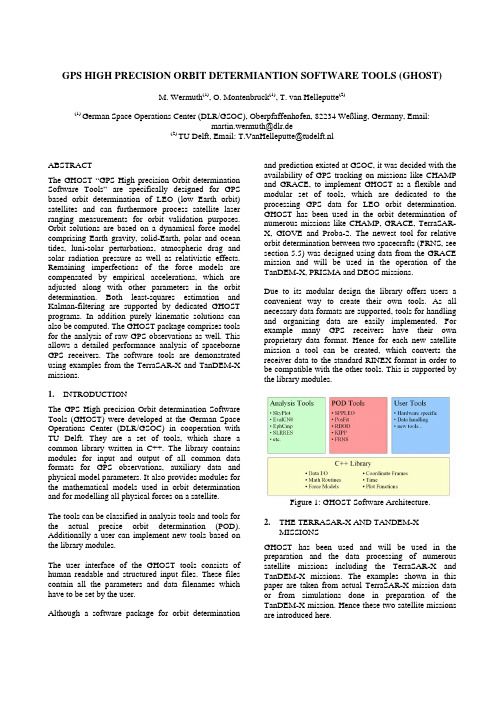
GPS HIGH PRECISION ORBIT DETERMIANTION SOFTWARE TOOLS (GHOST)M. Wermuth(1), O. Montenbruck(1), T. van Helleputte(2)(1) German Space Operations Center (DLR/GSOC), Oberpfaffenhofen, 82234 Weßling, Germany, Email:martin.wermuth@dlr.de(2) TU Delft, Email: T.VanHelleputte@tudelft.nlABSTRACTThe GHOST “GPS High precision Orbit determination Software Tools” are specifically designed for GPS based orbit determination of LEO (low Earth orbit) satellites and can furthermore process satellite laser ranging measurements for orbit validation purposes. Orbit solutions are based on a dynamical force model comprising Earth gravity, solid-Earth, polar and ocean tides, luni-solar perturbations, atmospheric drag and solar radiation pressure as well as relativistic effects. Remaining imperfections of the force models are compensated by empirical accelerations, which are adjusted along with other parameters in the orbit determination. Both least-squares estimation and Kalman-filtering are supported by dedicated GHOST programs. In addition purely kinematic solutions can also be computed. The GHOST package comprises tools for the analysis of raw GPS observations as well. This allows a detailed performance analysis of spaceborne GPS receivers. The software tools are demonstrated using examples from the TerraSAR-X and TanDEM-X missions.1.INTRODUCTIONThe GPS High precision Orbit determination Software Tools (GHOST) were developed at the German Space Operations Center (DLR/GSOC) in cooperation with TU Delft. They are a set of tools, which share a common library written in C++. The library contains modules for input and output of all common data formats for GPS observations, auxiliary data and physical model parameters. It also provides modules for the mathematical models used in orbit determination and for modelling all physical forces on a satellite.The tools can be classified in analysis tools and tools for the actual precise orbit determination (POD). Additionally a user can implement new tools based on the library modules.The user interface of the GHOST tools consists of human readable and structured input files. These files contain all the parameters and data filenames which have to be set by the user.Although a software package for orbit determination and prediction existed at GSOC, it was decided with the availability of GPS tracking on missions like CHAMP and GRACE, to implement GHOST as a flexible and modular set of tools, which are dedicated to the processing GPS data for LEO orbit determination. GHOST has been used in the orbit determination of numerous missions like CHAMP, GRACE, TerraSAR-X, GIOVE and Proba-2. The newest tool for relative orbit determination between two spacecrafts (FRNS, see section 5.5) was designed using data from the GRACE mission and will be used in the operation of the TanDEM-X, PRISMA and DEOS missions.Due to its modular design the library offers users a convenient way to create their own tools. As all necessary data formats are supported, tools for handling and organizing data are easily implemented. For example many GPS receivers have their own proprietary data format. Hence for each new satellite mission a tool can be created, which converts the receiver data to the standard RINEX format in order to be compatible with the other tools. This is supported by the library modules.Figure 1: GHOST Software Architecture.2.THE TERRASAR-X AND TANDEM-XMISSIONSGHOST has been used and will be used in the preparation and the data processing of numerous satellite missions including the TerraSAR-X and TanDEM-X missions. The examples shown in this paper are taken from actual TerraSAR-X mission data or from simulations done in preparation of the TanDEM-X mission. Hence these two satellite missions are introduced here.TerraSAR-X is a German synthetic aperture radar (SAR) satellite which was launched in June 2007 from Baikonur on a Dnepr rocket and is operated by GSOC/DLR. Its task is to collect radar images of the Earth’s surface. To support the TerraSAR-X navigation needs, the satellite is equipped with two independent GPS receiver systems. While onboard needs as well as orbit determination accuracies for image processing (typically 1m) can be readily met by the MosaicGNSS single-frequency receiver, a decimeter or better positioning accuracy must be achieved for the analysis of repeat-pass interferometry. To support this goal, a high-end dual-frequency IGOR receiver has been contributed by the German GeoForschungsZentrum (GFZ), Potsdam. Since the launch DLR/GSOC is routinely generating precise rapid and science orbit products using the observations of the IGOR receiver.In mid 2010 the TanDEM-X satellite is scheduled for launch. It is an almost identical twin of the TerraSAR-X satellite. Both satellites will fly in a close formation to acquire a digital elevation model (DEM) of the Earth’s surface by stereo radar data takes. Therefore the baseline vector between the two satellites has to be known with an accuracy of 1 mm. In preparation of the TanDEM-X mission, GHOST has been extended to support high precision baseline determination using single or dual-frequency GPS measurements.Figure 2: The TanDEM-X mission. (Image: EADSAstrium)3.THE GHOST LIBRARYThe GHOST library is written in C++ and fully object-oriented. All data objects are mapped into classes and each module contains one class. Classes are provided for data I/O, mathematical routines, physical force models, coordinate frames and transformations, time frames and plot functions.All data formats necessary for POD are supported by the library. Most important are the format for orbit trajectories SP3-c [1] and the ‘Receiver Independent Exchange Format’ RINEX [2] for GPS observations. The SP3 format is used for the input of GPS ephemerides (as those files are usually provided in SP3-c format) and for the output of the POD results. The raw GPS observations are provided in the RINEX format. At the moment the upgrade from RINEX version 2.20 to version 3.00 is ongoing to allow for the use of multi-constellation and multi-antenna files. Other data formats, which are supported, are the Antenna Exchange Format ANTEX [3] containing antenna phase center offsets and variations and the Consolidated Prediction Format CPF [4] used for the prediction of satellite trajectories to network stations. The Consolidated Laser Ranging Data Format CRD [5] which will replace the old Normal Point Data Format is currently being implemented.The library provides basic mathematical functions needed for orbit determination like a module for matrix and vector operations, statistical functions and quaternion algebra. As numerical integration plays a fundamental role in orbit determination, several numerical integration methods for ordinary differential equations are implemented, like the 4th-order Runge-Kutta method and the variable order variable stepsize multistep method of Shampine & Gordon [6].Forces acting on the satellite are computed by physical models including the Earth's harmonic gravity field, gravitational perturbations of the Sun and Moon, solid Earth and ocean tides, solar radiation pressure, atmospheric drag and relativistic effects.In orbit determination several coordinate frames are used. Most important are the inertial frame, the Earth fixed frame, the orbital frame and the spacecraft frame. The transformation between inertial and Earth fixed frame is quite complex as numerous geophysical terms like the Earth orientation parameters are involved. The orbital frame is defined by the position and velocity vectors of a satellite. The axes are oriented radial, tangential (along-track) and normal to the other axes and often denoted as R-T-N. The spacecraft frame is fixed to the mechanical structure of a satellite and used to express instrument coordinates (e.g. the GPS antenna coordinates). It is connect to the other frames via attitude information. The GHOST library contains transformations between all involved frames.Similar to reference frames, also several time scales like UTC and GPS time are involved in orbit determination.A module provides conversions between different time scales.In order to visualize results of the analysis tools or POD results like orbit differences or residuals, the librarycontains a module dedicated to the generation of post script plots.4.ANALYSIS TOOLSThe GHOST package comprises tools for the analysis of raw GPS observations and POD results. This allows a detailed performance analysis of spaceborne GPS receivers in terms of signal strength, signal quality, statistical distribution of observed satellites and hardware dependent biases. The tools can be used either to characterize the flight hardware already prior to the mission or to analyze the performance of in flight data during the mission. An introduction to the most important tools is given here.4.1.EphCmpOne of the most basic but most versatile tools is the ephemeris comparison tool EphCmp. It simply compares an orbit trajectory with a reference orbit and displays the differences graphically (see Fig. 3). The coordinate frame in which the difference is expressed can be selected. In addition a statistic of the differencesis given. It can be used to visualize orbit differences in various scenarios like the comparison of different orbit solutions, the comparison of overlapping orbit arcs or the evaluation of predicted orbits or navigation solutions against precise orbits.Figure 3: Comparison of two overlapping orbit arcsfrom TerraSAR-X POD.4.2.SkyPlotSkyPlot is a tool to visualize the geometrical distribution of observed GPS satellites in the spacecraft frame. A histogram and a timeline of the number of simultaneously tracked satellites are given as well. Hence the tool can be used to detect outages in the tracking.Fig. 4 shows the output of SkyPlot for the MosaicGNSS single-frequency receiver on TerraSAR-X on 2010/04/05. The antenna of the MosaicGNSS receiver is mounted with a tilt of 33° from the zenith direction. This is very well reflected in the geometrical distribution (upper left) of the observed GPS satellites. It can be seen, that mainly satellites in the left hemisphere have been tracked. The histogram (upper right) shows, that – although the receiver has 8 channels – most of the time only 6 satellites (or less) were tracked. The lower plot in Fig 4. shows the number of observed satellites as timeline. It can be seen, that there was a short outage of GPS tracking around 11h. This is useful information for the evaluation of GPS data and the quality of POD results.Figure 4: Distribution of tracked satellites by the MosaicGNSS receiver on TerraSAR-X.4.3.EvalCN0The tool EvalCN0 is used to analyze the tracking sensitivity of GPS receivers. It plots the carrier-to-noise ratio (C/N0) in dependence of elevation.The example shown in Fig. 5 is taken from a pre-flight test of the IGOR receiver on the TanDEM-X satellite. The test was carried out with a GPS signal simulator connected to the satellite in the assembly hall [7]. It can be seen, that under the given test-setup, the IGOR receiver achieves a peak carrier-to-noise density ratio (C/N0) of about 54 dB-Hz in the direct tracking of the L1 C/A code. The C/N0 decreases gradually at lower elevations but is still above 35 dB-Hz near the cut-off elevation of 10°.For the semi-codeless tracking of the encrypted P-code, the C/N0 values S1 and S2 reported by the IGOR receiver on the L1 and L2 frequency show an even stronger decrease towards the lower elevations. The signal strength of the L2 frequency is about 3dB-Hzlower than that for the L1 frequency. To evaluate the semi-codeless tracking quality, the size of the S1-SA and S2-SA difference is shown in the right plot of Fig.5. Both frequencies show an expected almost linear variation compared to SA. The degradation of the signal due to semi-codeless squaring losses increases with lower elevation.Figure 5: Variation of C/N0 with the elevation of the tracked satellite (left) and semi-codeless tracking losses (right) forthe pre-flight test of the IGOR receiver on TanDEM-X.4.4.SLRRESSatellite Laser Ranging (SLR) is an important tool for the evaluation of the quality of GPS-based precise satellite orbits. It is often the only independent source of observations available, with an accuracy good enough to draw conclusions about the accuracy of the precise GPS orbits.SLRRES computes the residual of the observed distance between satellite and laser station versus the computed distance. The residuals are displayed in a plot (see Fig.6). As output daily statistic, station-wide statistics and an overall RMS residual are given.In order to compute the distance between satellite and laser station, the orbit position of the satellite has to be corrected for the offset of the satellites laser retro reflector (LRR) from the center of mass using attitude information. The coordinates of the laser station are taken from a catalogue and have to be transformed to the epoch of the laser observation. This is done by applying corrections for ocean loading, tides, and plate tectonics. Finally the path of the laser beam has to be modelled considering atmospheric refractions and relativistic effects.Figure 6: SLR Residuals of TerraSAR-X POD forMarch 2010.5.PRECISE ORBIT DETERMINATION TOOLSThe POD tools comprise two different fundamental methods of orbit determination. A reduced-dynamic orbit determination is computed by the RDOD tool, while KIPP produces a kinematic orbit solution. Both tools process the carrier phase GPS observations. They need a reference solution to start with. This is provided by the tools SPPLEO and PosFit.SPPLEO generates a coarse navigation solution by processing the pseudorange GPS observations. The satellite position and receiver clock offset are determined in a least squares adjustment. Next PosFit is run to determine a solution in case of data gaps and to smoothen the SPPLEO solution by taking the satellite dynamics into account.5.1.SPPLEOSPPLEO (Single Point Positioning for LEO satellites) is a kinematic least squares estimator for LEO satellites processing pseudorange GPS observations. The program produces a first navigation solution, with data gaps still present. For each epoch, the satellite position and receiver clock offset are determined in a least-squares adjustment.The tool is able to handle both single and dual-frequency observations. In case of single frequency observations, the C1 code is used without ionosphere correction. In case of dual-frequency observations, the ionosphere free linear combination of P1 and P2 code observations is applied. In case range-rate observations are available, it is also possible to estimate velocities. Before the adjustment, the data is screened and edited. Hence the user can choose hard editing limits for the signal to noise ratio of the observation, the elevation and the difference between code and carrier phase observation. In case of the violation of one limit, the observation is rejected. If the number of observations for one epoch is below the limit set by the user, the whole epoch is rejected. After the adjustment the PDOP is computed, and if it exceeds a limit, the epoch is rejected as well. If the a posteriori RMS of the residuals exceeds the threshold set by the user, the observation yielding the highest value is rejected. This is repeated until the RMS is below the threshold or the number of observations is below the limit.The resulting orbit usually contains data gaps and relatively large errors compared to dynamic orbit solutions. Hence the gaps have to be closed and the orbit has to be smoothed by the dynamic filter tool PosFit.5.2.PosFitPosFit is a dynamic ephemeris filter for processing navigation solutions as those produced by SPPLEO. This is done by an iterated weighted batch least squares estimator with a priori information. The batch filter estimates the initial state vector, drag and solar radiation coefficients. In addition to those model parameters, empirical accelerations are estimated. One empirical parameter is determined for each of the three orthogonal components of the orbital frame (radial, along-track and cross-track) for an interval set by the user. The parameters are assumed to be uncorrelated over those intervals.The positions of the input navigation solution are introduced as pseudo-observations. The filter is fitting an integrated orbit to the positions of the input orbit in an iterative process. In order to obtain initial values for the first iteration, Keplerian elements are computed from the first two positions of the input orbit. All forces that act on the satellite (like atmospheric drag, solar radiation pressure, tides, maneuvers…) are modelled and applied in the integration. Due to imperfections in the force models, the empirical accelerations are introduced, to give the integrated orbit more degrees of freedom, to fit to the observations. The empirical acceleration parameters are estimated in the least squares adjustment together with the initial state vector and model parameters. The partial derivatives of the observations w.r.t. the unknown parameters are obtained by integration of the variational equations along the orbit (for details see [8]). The result of PosFit is a continuous and smooth orbit without data gaps in SP3-c format. It can serve as reference orbit for RDOD and KIPP.Figure 7 displays the graphical output of PosFit. The three upper graphs show the residuals after the adjustment in the three components of the orbital frame. In this example, which is taken from a 30h POD arc of the TerraSAR-X mission, the RMS of the residuals lies between 0.5m and 1.5m. This mainly shows the dispersion of positions of the SPPLEO solution. The three lower graphs show the estimated empirical accelerations in the three components of the orbital frame.Figure 7: Graphical output of PosFit Tool forTerraSAR-X POD.5.3.RDODRDOD is a reduced dynamic orbit determination tool for LEO satellites processing carrier phase GPS observations. This is also done by an iterated weighted batch least squares estimator with a priori information. Similar to PosFit, RDOD estimates the initial state vector, drag and solar radiation coefficients and empirical accelerations. Contrary to PosFit, where the positions of a reference orbit are used as pseude-observations, RDOD directly uses the GPS pseudorange and carrier phase observations. Nevertheless a continuous reference orbit – normally computed by PosFit – is required by RDOD for data editing and for obtaining initial conditions for the first iteration.The tool is able to handle both single and dual-frequency data. In case of single frequency observations, the GRAPHIC (Group and Phase Ionospheric Correction) combination of C/A code and L1 carrier-phase is used as observation. In case of dual-frequency observations, the ionosphere free linear combination of L1 and L2 carrier phase observations is applied.The data editing is crucial to the quality of the results. Hence the data is also screened and edited by RDOD using limits specified by the user. If the signal-to-noise ratio of the observation exceeds the limit, or the elevation is below a cut-off elevation, the observation is rejected. This is done if no GPS ephemerides and clock information is available for that observation. Next outliers in the code and carrier-phase observations are detected. This is done comparing the observations to modelled observations using the reference orbit.The RDOD filter is fitting an integrated orbit to the carrier-phase observations. This is done in a similar way as in PosFit, considering all forces on the satellite and estimating empirical acceleration parameters. But while PosFit uses absolute positions as observations, the carrier-phase observations used in RDOD contain an unknown ambiguity. The ambiguity is considered to be constant over one pass – the time span in which a GPS satellite is tracked continuously. Hence one unknown ambiguity parameter per pass is added to the adjustment.The graphical output of RDOD shows the residuals of the code and carrier phase observations (see Fig. 8). This is an important tool for a fast quality analysis and for detecting systematic errors.Figure 8: Output of RDOD tool for TerraSAR-X POD.Both the antennas of the GPS satellites and the GPS antennas of spaceborne receivers show variations of the phase center dependent on azimuth and elevation of the signal path. It is necessary to model those variations in order to obtain POD results with highest quality. GHOST does not only offer the possibility to use phase center variation maps given in ANTEX format. It also offers the possibility to estimate such phase center variation patterns, and thus can be employed for the in-flight calibration of flight hardware. This was done for the GPS on TerraSAR-X as shown in Fig. 9. The figure shows the phase center variation pattern for the main POD antenna of the IGOR receiver on TerraSAR-X. It was estimated from 30 days of flight data and needs to be applied to carrier phase observations in addition to a pattern which was determined for the antenna type by ground tests (for details cf. [9]).Figure 9: Phase Center Variation Pattern for the MainPOD Antenna on TerraSAR-X.5.4. KIPPKIPP (Kinematic Point Positioning) is a kinematic least squares estimator for LEO satellites. Similar to RDOD carrier phase observations are processed. But in contrast to RDOD no dynamic models are employed, and only the GPS observations are used for orbit determination. For each epoch, the satellite position and receiver clock offset are determined in a weighted least squares adjustment. KIPP also requires a continuous reference orbit, as that computed by PosFit.Like RDOD, the KIPP tool is able to handle both single and dual-frequency data. In case of single frequency observations, the GRAPHIC (Group and Phase Ionospheric Correction) combination of C/A code and L 1 carrier-phase is used as observation. In case of dual-frequency observations, the ionosphere free linear combination of L 1 and L 2 carrier phase observations is applied.5.5. FRNSThe Filter for Relative Navigation of Satellites (FRNS) is designed to perform relative orbit determination between two LEO spacecrafts. This is done using an extended Kalman filter described in [10]. The concept is to achieve a higher accuracy for the relative orbit between two spacecrafts by making use of differenced GPS observations, than by simply differencing two independent POD results. FRNS requires a continuous reference orbit for both spacecrafts, such as computed by RDOD. It then keeps the orbit of one spacecraft fixed, determines the relative orbit between the two spacecrafts and adds it to the positions of the first spacecraft. As result a SP3-c file containing the orbit of both spacecrafts is obtained. The tool is able to process both single and dual-frequency observations.The FRNS tool was developed using data from the GRACE mission and will be applied on a routine basis for the TanDEM-X mission. In contrast to TanDEM-X, GRACE consists of two spacecrafts, which follow each other on a similar orbit with about 200 km distance. The distance between the two spacecrafts is measured by a K-band link, which is considered to be at least one order of magnitude more accurate than GPS observations. Hence the K-band observations can be used to assess the accuracy of the relative navigation results – with the limitation, that the K-band observations only reflect the along-track component, and contain an unknown bias. The differences between a GRACE relative navigation solution and K-band observations are shown in Fig. 10. The standard deviation is about 0.7 mm. As the TanDEM-X mission uses GPS receivers which are follow-on models of those used on GRACE, and the distance between the spacecrafts is less than 1 km, one can expect that the quality of the relative orbit determination will be on the same level of accuracy or even better.Figure 10: Comparison of GRACE relative navigation solution with K-band observations.6.REFERENCES1. Hilla S. (2002). The Extended Standard Product 3Orbit Format (SP3-c, National Geodetic Survey,National Ocean Service, NOAA.2. Gurtner W., Estey L. (2007). The ReceiverIndependent Exchange Format Version 3.00,Astronomical Institute University of Bern.3. Rothacher M., Schmid R. (2006). ANTEX: TheAntenna Exchange Format Version 1.3,Forschungseinrichtung Satellitengeodäsie TUMünchen.4. Rickfels R. L. (2006). Consolidated Laser RangingPrediction Format Version 1.01, The University of Texas at Austin/ Center for Space Research.5. Rickfels R. L. (2009). Consolidated Laser RangingData Format (CRD) Version 1.01, The Universityof Texas at Austin/ Center for Space Research. 6. Shampine G. (1975). Computer solution of OrdinaryDifferential Equations, Freeman and Comp., SanFrancisco.7. Wermuth M. (2009). Integrated GPS Simulator Test,TanDEM-X G/S-S/S Technical Validation Report,Volume 15: Assembly AS-1515, DLROberpfaffenhofen.8. Montenbruck O., Gill E. (2000). Satellite Orbits –Models, Methods and Applications, Springer-Verlag, Berlin, Heidelberg, New York.9. Montenbruck O. Garcia-Fernandez M., Yoon Y.,Schön S., Jäggi A..; Antenna Phase CenterCalibration for Precise Positioning of LEOSatellites; GPS Solutions (2008). DOI10.1007/s10291-008-0094-z.10. Kroes R. (2006). Precise Relative Positioning ofFormation Flying Spacecraft using GPS, PhDThesis, TU Delft.。

多粒度模糊粗糙集的表示与相应的信任结构

多粒度模糊粗糙集的表示与相应的信任结构胡谦;米据生【摘要】利用多粒度粗糙集的上、下近似及其性质,结合模糊集的分解定理,研究多粒度模糊粗糙集的上、下近似的表示及性质,根据多粒度模糊粗糙集的上、下近似构造信任函数与似然函数.%By using the upper and lower approximations and the properties of the multi-granularity rough sets, and combining with fuzzy sets decomposition theorem, the representation and properties of upper and lower approximations of multi-granularity fuzzy rough sets are studied. Based on the upper and lower approximations of fuzzy rough sets, the belief function and the probability function are constructed.【期刊名称】《计算机工程与应用》【年(卷),期】2017(053)019【总页数】4页(P51-54)【关键词】多粒度;粗糙集;模糊集;信任函数;似然函数【作者】胡谦;米据生【作者单位】河北师范大学数学与信息科学学院,石家庄 050024;河北师范大学数学与信息科学学院,石家庄 050024【正文语种】中文【中图分类】O236自1965年Zadeh教授提出模糊集[1]的概念以来，模糊数学在理论与应用方面都得到了迅速的发展。

波兰数学家Pawlaw于1982年提出粗糙集理论，它是一种处理信息不完备，不精确的有效数学工具[2-3]，其方法在知识发现中的作用日益显著。

近年来，把二者结合用于研究实际问题中的不确定性成为粗糙集与模糊集研究的主流方向之一[4-5]。

Granular Computing

Granular ComputingY.Y. YaoDepartment of Computer Science, University of ReginaRegina, Saskatchewan, Canada S4S 0A2E-mail: yyao@cs.uregina.ca, http://www.cs.uregina.ca/~yyaoAbstract The basic ideas and principles of granular computing (GrC) have been studied explicitly or implicitly in many fields in isolation. With the recent renewed and fast growing interest, it is time to extract the commonality from a diversity of fields and to study systematically and formally the domain independent principles of granular computing in a unified model. A framework of granular computing can be established by applying its own principles. We examine such a framework from two perspectives, granular computing as structured thinking and structured problem solving. From the philosophical perspective or the conceptual level, granular computing focuses on structured thinking based on multiple levels of granularity. The implementation of such a philosophy in the application level deals with structured problem solving.Keywords: Granularity, granule, level, hierarchy, structured thinking, structured problem solving1. IntroductionHuman problem solving involves the perception, abstraction, representation and understanding of real world problems, as well as their solutions, at different levels of granularity [4, 6, 23, 28, 32-35]. The consideration of granularity is motivated by the practical needs for simplification, clarity, low cost, approximation, and tolerance of uncertainty [32]. As an emerging field of study, granular computing attempts to formally investigate and model the family of granule-oriented problem solving methods and information processing paradigms [14, 23, 28].Ever since the introduction of the term of “Granular computing (GrC)” by T.Y. Lin in 1997 [8, 32], we have witnessed a rapid development of and a fast growing interest in the topic [2, 5, 8-10, 13, 14,16-20, 22-31, 33, 35, 37]. Many models and methodsof granular computing have been proposed and studied. From the wide spectrum of current research, one can easily make several observations. There does not exist a general agreement about what is granular computing, nor there is a unified model [36]. Many studies concentrate on concrete models in particular contexts, and hence only capture limited aspects of granular computing. Consequently, the potential applicability and usefulness of granular computing are not well perceived and appreciated.The studies of concrete models and methods are important for the development of a field in its early stage. It is equally important, if not more, to study a general theory that avoids constraints of a concrete model.The basic notions and principles of granular computing, though under different names, have in fact been appeared in many related fields, such as programming, artificial intelligence, divide and conquer, interval computing, quantization, data compression, chunking, cluster analysis, rough set theory, quotient space theory, belief functions, machine learning, databases, and many others [8, 23, 28, 32, 33]. However, granular computing has not been fully explored in its own right. It is time to extract the commonality from these diverse fields andto study systematically and formally the domain independent principles of granular computing in a unified and well-formulated framework.In this paper, we study high level and qualitative characteristics of a theory of granular computing. A general domain independent framework is presented,in which basic issues are examined.2. Perspectives of Granular ComputingIt may be difficult, if not impossible, to give a formal, precise and uncontroversial definition of granular computing. N evertheless, one can still extract the fundamental elements from the human problem solving experiences and methods. There are basic principles, techniques and methodologies that are commonly used in most types of problem solving. Granular computing, therefore, focuses on problem solving based on the commonsense concepts of granule, granulated view, granularity, and hierarchy. They are interpreted as the abstraction, generalization, clustering, levels of abstraction, levelsof detail, and so on in various domains. We view granular computing as a study of a general theory of problem solving based on different levels of granularity and detail [28].Granular computing can be studied by applying its principles and ideas. It can be investigated in different levels or perspectives by focusing on itsphilosophical foundations, basic components, fundamental issues, and general principles. The philosophical level concerns structured thinking, and the application level deals with principles of structured problem solving. While structured thinking provides guidelines and leads naturally to structured problem solving, structured problem solving implements the philosophy structured thinking.The philosophy of thinking in terms of levels of granularity, and its implementation in more concrete models, would result in disciplined procedures that help to avoid errors and to save time for solving a wide range of complex problems.3. Basic Components of Granular ComputingIn modeling granular computing, we focus on three basic components and their interactions.3.1. GranulesA granule may be interpreted as one of the numerous small particles forming a larger unit. Collectively, they provide a representation of the unit with respect to a particular level of granularity. That is, a granule may be considered as a localized view or a specific aspect of a large unit.Granules are regarded as the primitive notion of granular computing. Its physical meanings become clearer when dealing with more concrete models. For example, in set-theoretic setting, such as rough sets, quotient space theory and cluster analysis, a granule may be interpreted as a subset of a universal set [12, 13, 34, 35]. In planning, a granule can be a sub-plan [6]. In programming, a granule can be a program module [7]. For the conceptual formulation of granular computing, we do not attempt to interpret the notion of granules based on more intuitive, but rather restrictive, concepts. We focus on some fundamental issues based on this weak view of granules.The size of a granule is considered as a basic property. Intuitively, the size may be interpreted as the degree of abstraction, concreteness, or detail. In the set-theoretic setting, the size of a granule can be the cardinality of the granule.Connections and relationship between granules can be represented by binary relations. In concrete models, they may be interpreted as dependency, closeness, or overlapping. For example, based on the notion of size, one can define an order relation on granules. Depending on the particular context, the relation may be interpreted as “greater than or equal to”, “more abstract than”, or “coarser than”. The order relation may be reflexive and transitive, but not symmetric. The order relation is particularly useful in studying connections between granules in different levels.One can define operations on granules so that one can operate on granules, such as combining many granules to form a new granule or decomposing a granule into many granules. The operations on granules must be consistent with the binary relations on the granules. For example, the combined granule should be more abstract than its components. The sizes of granules, the relations between granules, and the operations on granules provide the essential ingredients for developing a theory of granular computing.3.2. Granulated views and levelsIn his work on vision, Marr convincingly made the point that a full understanding of an information processing system involves explanations at various levels [11]. The three levels considered are the computational, algorithmic, and implementational. The computational level describes the information processing problem to be solved by the system. The algorithmic level describes the steps that need to be carried out to solve the problem. The implementational level deals with physical realization of the system. Although there does exist a general agreement on the interpretations and the exact number of levels, it is commonly accepted that the notion of levels is an important one in computer science [3].Foster critically reviewed and systematically compared various definitions and interpretations of the notion of levels [3]. Three basic issues, namely, definition of levels, number of levels, and relationship between levels, are clarified. Levels are considered simply as descriptions or points of views and often for the purpose of explanation. The number of levels is not fixed, but depends on the context and the purpose of description or explanation.A multi-layered theory of levels captures two senses of abstraction. One is the abstraction in terms of concreteness and is represented by planes along the dimension from top to bottom. The other is the abstraction in terms of the amount of detail and can be modeled along another dimension from less detail to more detail on the same plane.By viewing a level as a description or a point of view, one can immediately apply it as a basic notion to model granular computing. In order to emphasize the context of granular computing, we also refer to a level as a granulated view. A level consists of entities called granules whose properties characterize and describe the subject matters of study, such as a real world problem, a theory, a design, a plan, a program, or an information processing system. Granules are formed with respect to a particular degree of granularity or detail. Granules in a level are defined and formed within a particular context and are related to granules in other levels.There are two types of information and knowledge encoded in a level. A granule captures a particular aspect, and collectively, all granules in the level provide a granulated view. The granularity of a level refers to the collective properties of granules in a level with respect to their sizes. The granularity is reflected by the sizes of all granules involved.3.3. HierarchiesGranules in different levels are linked by the order relations and operations on granules. The order relation on granules can be extended to granulated views (levels). A level is above another level if each granule in the former level is ordered before a granule in the latter level, and each granule in the latter level is ordered after a granule in the former level, under the order relation. The ordering of levels can be described by the notion of hierarchy.The theory of hierarchy provides a multi-layered framework based on levels. Mathematically, a hierarchy may be viewed as a partially ordered set [1]. For the study of granular computing, the elements of the ordered set are interpreted as hierarchical levels or granulated views. The ordering of levels in a hierarchy is based on criteria that are related to the order relations on granules. A higher level may provide a constraint to and/or context of a lower level, and may contain and be made of lower levels. Depending on the context, a hierarchy may consist of levels of interpretation, levels of abstraction, levels of organization, levels of observation, and levels of detail. A hierarchy represents relationships between different granulated views, and explicitly shows the structure of granulation.A granule in a higher level can be decomposed into many granules in a lower level, and conversely many granules in a lower level can be combined into one granule in a higher level. A granule in a lower level may be a more detailed description of a granule in a higher level with added information. In the other direction, a granule in a higher level is a coarse-grained description of a granule in a lower level by omitting irrelevant details.3.4. Granular structuresWith the introduction of the three components, one can examine three types of structures for modeling their interactions. They are the internal structure of a granule, the collective structure of the all granules (i.e., the internal structure of a granulated view or level), and the overall structure of all levels.Although a granule is normally considered as a whole instead of many sub-granules at a given level, its internal structure needs to be examined. The internal structure of a granule provides a proper description, interpretation, and characterization of the granule. A granule may have a complex structure itself. For examples, the internal structure of a granule may be a hierarchy consisting of many levels. The internal structure is also useful in establishing linkage among granules in different levels.All granules in a level may collectively show a certain structure. This is the internal structure of a granulated view. Granules in a level, although may be relatively independent, are somehow related to a certain degree. This stems from the fact that they together form a granulated view. On the other hand, it is expected that in many situations the relationships between different granules are much weaker. The internal structure of a level is only meaningful if all the granules in the level are considered together.A hierarchy represents the overall structure of all levels. In a hierarchy, both the internal structure of granule and the internal structure of granulated views are reflected, to some degree, by the order relations. In a hierarchy, not any two granulated views can be compared based on the order relation. In the special case, the hierarchy is a tree.The three structures as a whole is referred to as the granular structure. One can establish more connections between three structures. For example, granules in a higher level may have greater integrity and higher bond strength than those in a lower level. The structures need to be fully explored to establish a basis of granular computing.3.5. A partition modelThe three basic components of granular computing can be easily illustrated by a concrete model known as the partition model of granular computing [28], which is based on rough set theory [12, 13] and quotient space theory [34, 35].A central notion of the partition model is equivalence relations. In rough set theory, an equivalence relation on a set of objects can be concretely defined in an information table based on their values on a finite set of attributes [12, 31]. Two objects are equivalent if they have exact the same values on a set of attributes.An equivalence relation divides a universal set into a family of pair-wise disjoint subsets, called the partition of the universe. A granule of a partition model is therefore an equivalence class defined by an equivalence relation. The internal structure of an equivalence class is captured by the same values of some attributes. A granulated view is the partition induced by an equivalence relation, and its structure is defined by the properties of the partition. Different equivalence relations can be ordered based on set inclusion, which leads to a hierarchy of partitions. In an information table, we only consider partitions generated by different subsets of attributes. The overall hierarchical structure is therefore induced bysubsets of attributes.The partition model may be viewed as a special case of cluster analysis. Following the same argument, one can easily find the correspondence between basic components of granular computing and its structures in cluster analysis. In general, given any concrete model of granular computing, we can easily find the corresponding components and structures.4. Basic Issues of Granular ComputingThe discussions of this section summarize and extend the preliminary results reported in [23, 28]. The list of issues discussed should not be viewed as a complete one. It can only be viewed as a set of representatives. Based on the principles of granular computing, these issues may also be studied at different levels of detail.Granular computing may be studied based on two related issues, i.e., granulation and computation 23, 28]. The former deals with the construction, interpretation, and representation of the three basic components, and the latter deals with the computing and reasoning with granules and granular structures.Studies of granular computing cover two perspectives, namely, the algorithmic and the semantic [23, 28]. Algorithmic study concerns the procedures for constructing granules and related computation, and the semantic study concerns the interpretation and physical meaningfulness of various algorithms. Studies from both aspects are necessary and important. The results from semantic study may provide not only interpretations and justifications for a particular granular computing model, but also guidelines that prevent possible misuses of the model. The results from algorithmic study may lead to efficient and effective granular computing methods and tools.4.1. GranulationGranulation involves the construction of the three basic components, granules, granulated views and hierarchies. Two basic operations are the top-down decomposition of large granules to smaller granules, or the bottom-up combination of smaller granules into larger granules.The notion of granulation can be studied in many different contexts. The granulation of a problem, a theory, or a universe, particularly the semantics of granulation, is domain and application dependent. Nevertheless, one can still identify some domain independent issues. For clarity, some of these issues are discussed in the set-theoretic setting.In the set-theoretic setting, a granule may be viewed as a subset of the universe, which may be either fuzzy or crisp. A family of granules containingevery object in the universe is called a granulatedview of the universe. A granulated view may consistof a family of either disjoint or overlapping granules.There are many granulated views of the same universe. Different views of the universe can belinked together, and a hierarchy of granulated viewscan be established.Granulation criteria. A granulation criteriondeals with the semantic issues and addresses the question of why two objects are put into the same granule. It is domain specific and relies on the available knowledge. In many situations, objects are usually grouped together based on their relationships,such as indistinguishability, similarity, proximity, or functionality [32]. One needs to build models to provide both semantical and operational interpretations of these notions. They enable us to formally and precisely define various notions involved, and to systematically study the meaningsand rationale of a granulation criterion.Granulation methods. From the algorithmic aspect, a granulation method addresses the problemof how to put two objects into the same granule. It is necessary to develop algorithms for constructing granules and granulated views efficiently based on a granulation criterion.Representation/description. The next issue isthe interpretation of the results of a granulation method, i.e., the granular structures. Once constructed, it is necessary to describe, to name andto label granules using certain languages. One may assign a name to a granule such that an element in the granule is an instance of the named category. Onemay also provide a formal description of objects inthe same granule. By pooling the representations of granules, one can obtain the overall representation ofa granulated view.Qualitativ e and quantitativ e characterization.One can associate quantitative measures to the three components, granules, granulated views, and hierarchies. The measures should reflect and be consistent with the three structures, the internal structure of a granule, the collective structure of a granulated view, and the overall structure of a hierarchy.4.2. Computing with granulesComputing and reasoning with granules explorethe three types of structures. They can be similarly studied from both the semantic and algorithmic perspectives. One needs to design and interpret various methods based on the interpretation of granules and relationships between granules, as wellas to define and interpret operations of granular computing.Mappings. The connections between differentlevels of granulations can be described by mappings. At each level of the hierarchy, a problem is represented with respect to the granularity of the level. The mapping links different representations of the same problem at different levels of detail. In general, one can classify and study different types of granulations by focusing on the properties of the mappings.Granularity conversion. A basic task of granular computing is to change views with respect to different levels of granularity. As we move from one level of detail to another, we need to convert the representation of a problem accordingly. A move to a more detailed view may reveal information that otherwise cannot be seen, and a move to a simpler view can improve the high level understanding by omitting irrelevant details of the problem.Operators. Operators can precisely define the conversion of granularity in different levels. They serve as the basic building blocks of granular computing. There are at least two types of operators that can be defined. One type deals with the shift from a fine granularity to a coarse granularity. A characteristic of such an operator is that it will discard certain details, which makes distinct objects no longer differentiable. Depending on the context, many interpretations and definitions are available, such as abstraction, simplification, generalization, coarsening, zooming-out, and so on. The other type deals with the change from a coarse granularity to a fine granularity. A characteristic of such an operator is that it will provide more details, so that a group of objects can be further classified. They can be defined and interpreted differently, such as articulation, specification, expanding, refining, zooming-in, and so on.Property preservation. Granulation allows different representations of the same problem in different levels of detail. It is naturally expected that the same problem must be consistently represented. Granulation and its related computing methods are meaningful only if they preserve certain desired properties. For example, Zhang and Zhang studied the “false-preserving” property, which states that if a coarse-grained space has no solution for a problem then the original fine-grained space has no solution [34, 35]. Such a property can be explored to improve the efficiency of problem solving by eliminating a more detailed study in a coarse-grained space. One may require that the structure of a solution in a coarse-grained space is similar to the solution in a fine-grained space. Such a property is used in top-down problem solving techniques. More specifically, one starts with a sketched solution and successively refines it into a full solution. In the context of hierarchical planning, one may impose similar properties, such as upward solution property, downward solution property, monotonicity, etc. [6]. 4.3. The rough set modelAs an illustration, we discuss the basic issues of granular computing based on the results from the rough set theory. Many applications of the rough set theory are based on the exploration of those issues.Granulation. The granulation criterion is an equivalence relation on a set of objects, which is concretely defined in an information table based on the values of a set of attributes. The granulation method is simply the collection of equivalent objects. One associates a formula to each equivalence class, which provides a formal description of the equivalence class. One also associates quantitative measures to equivalence classes and the partition induced by the equivalence relation.Computing with granules. Many of the applications of rough set theory can be viewed as concrete examples of computing with granules. With respect to an information table, mappings between different granulated views are in fact defined by different subsets of attributes. The conversion of granularity is achieved by adding or deleting attributes. The rough set approximation operators are granularity conversion operators.An important application of rough set theory is to learn classification rules [12, 21]. One of the important steps is to find a reduct of attributes, i.e., a set of individually necessary and collectively sufficient attributes that provide the correct classification [12, 21]. Conceptually, this can be easily modeled as searching the partition hierarchy defined by all subsets of attributes. Even in this simple search process, we have to deal with the issues discussed earlier. The mappings between levels direct the search direction; granularity conversion and property preserving principles govern the quality of the searched granulated views, the operators can be used to define the quality of each decision rule.5. ConclusionBy explicitly introducing an umbrella term of granular computing, one can explore, organize and unify the divergent concepts, theories, and applications into a well-formulated and unified theory of problem solving. It is time to move from studies of particular methods and concrete models of granular computing to a more abstract level. One needs to study its basic philosophy and principles, and to build a more general framework. This paper may be viewed as a step toward this goal.Although this paper does not cover all aspects of a complete model of granular computing, the results are useful in building a concrete model in which one can examine specific techniques and issues of granular computing in the context of particularapplications.The notions of granules, granulated views (levels) and hierarchies are sufficient for us to discuss the basic issues of granular computing. The sizes of granules, the granular structures, and the operations on granules provide the essential ingredients for the development of a theory of granular computing. References1.Ahl, V. and Allen, T.F.H. (1996) Hierarchy Theory, aision, V ocabulary and Epistemology, Columbia University Press.2.Bargiela, A. and Pedrycz W. (2002) GranularComputing: an Introduction,Kluwer Academic Publishers, Boston.3.Foster, C.L. (1992) Algorithms, Abstraction andImplementation: Levels of Detail in Cognitive Science,Academic Press, London.4.Hobbs, J.R. (1985) Granularity, Proceedings of the 9thInternational Joint Conference on Artificial Intelligence, 432-435.5.Inuiguchi, M., Hirano, S. and Tsumoto, S. (Eds.)(2003) Rough Set Theory and Granular Computing,Springer, Berlin.6.Knoblock, C.A. (1993) Generating AbstractionHierarchies: an Automated Approach to ReducingSearch in Planning, Kluwer Academic Publishers,Boston.7.Ledgard, H.F., Gueras, J.F. and N agin, P.A. (1979)PASCAL with Style: Programming Proverbs, HaydenBook Company, Inc., Rechelle Park, New Jersey.8.Lin, T.Y. (1997) Granular computing, announcementof the BISC Special Interest Group on GranularComputing.9.Lin, T.Y. (2003) Granular computing, LN CS 2639,Springer, Berlin, 16-24.10.Lin, T.Y., Yao, Y.Y. and Zadeh, L.A. (Eds.) (2002)Data Mining, Rough Sets and Granular Computing,Physica-Verlag, Heidelberg.11.Marr, D. (1982) V ision: A ComputationalInvestigation into the Human Representation andProcessing of Visual Information, W.H. Freeman andCompany, New York.12.Pawlak, Z. (1991) Rough Sets, Theoretical Aspects ofReasoning about Data, Kluwer Academic Publishers,Dordrecht.13.Pawlak, Z. (1998) Granularity of knowledge,indiscernibility and rough sets, Proceedings of 1998IEEE International Conference on Fuzzy Systems,106-110.14.Pedrycz, W. (Ed.), 2001, Granular Computing: anEmerging Paradigm, Physica-Verlag, Heidelberg.15.Peikoff, L. (1981) Objectivism: the Philosophy of AynRand, Dutton, New York.16.Peters, J.F., Pawlak, Z. and Skowron, A. (2002) Arough set approach to measuring information granules,Proceedings of COMPSAC 2002, 1135-1139.17.Polkowski, L. and Skowron, A. (1998) Towardsadaptive calculus of granules, Proceedings of 1998IEEE International Conference on Fuzzy Systems,111-116.18.Skowron, A. (2001) Toward intelligent systems:calculi of information granules, Bulletin of International Rough Set Society, 5, 9-30.19.Skowron, A. and Stepaniuk, J. (2001) Informationgranules: towards foundations of granular computing,International Journal of Intelligent Systems, 16, 57-85.20.Wang, G., Liu, Q., Yao, Y.Y. and Skowron, A. (Eds.)(2003) Rough Sets, Fuzzy Sets, Data Mining, andGranular Computing, LNCS 2639, Springer, Berlin. 21.Wang, J. (2002), Rough sets and their applications indata mining, in: Fuzzy Logic and Soft Computing,Chen, G., Ying, M. and Cai, K.-Y. (Eds.), KluwerAcademic Publishers, Boston.22.Yao, Y.Y., (1999) Granular computing usingneighborhood systems, in: Advances in Soft Computing: Engineering Design and Manufacturing,Roy, R., Furuhashi, T., and Chawdhry, P.K. (Eds),Springer-Verlag, London, 539-553.23.Yao, Y.Y. (2000) Granular computing: basic issuesand possible solutions, Proceedings of the 5th JointConference on Information Sciences, 186-189.24.Yao, Y.Y. (2001) Information granulation and roughset approximation, International Journal of IntelligentSystems, 16, 87-104.25.Yao, Y.Y. (2001) Modeling data mining with granularcomputing, Proceedings of COMPSAC 2001, 638-643.26.Yao, Y.Y. (2003) Information granulation andapproximation in a decision-theoretical model of rough sets, in: Rough-Neural Computing: Techniquesfor Computing with Words, Pal, S.K., Polkowski, L.,and Skowron, A. (Eds), Springer, Berlin, 491-518.27.Yao, Y.Y. (2003) Granular computing for the designof information retrieval support systems, in: Information Retrieval and Clustering, Wu, W., Xiong,H. and Shekhar, S. (Eds.), Kluwer AcademicPublishers 299.28.Yao, Y.Y. (2004) A partition model of granularcomputing, LNCS Transactions on Rough Sets, toappear.29.Yao, Y.Y. and Liau, C.-J. (2002) A generalizeddecision logic language for granular computing, Proceedings of FUZZ-IEEE'02, 1092-1097.30.Yao, Y.Y., Liau, C.-J. and Zhong, N. (2003) Granularcomputing based on rough sets, quotient space theory,and belief functions, Proceedings of ISMIS'03, 152-159.31.Yao, Y.Y. and Zhong, N. (2002) Granular computingusing information tables, in: Data Mining, Rough Setsand Granular Computing, Lin, T.Y., Yao, Y.Y. andZadeh, L.A. (Eds.), Physica-Verlag, Heidelberg, 102-124.32.Zadeh, L.A. (1997) Towards a theory of fuzzyinformation granulation and its centrality in humanreasoning and fuzzy logic, Fuzzy Sets and Systems, 19,111-127.33.Zadeh, L.A. (1998) Some reflections on softcomputing, granular computing and their roles in theconception, design and utilization of information/ intelligent systems, Soft Computing, 2, 23-25.34.Zhang, B. and Zhang, L. (1992) Theory andApplications of Problem Solving, N orth-Holland, Amsterdam.35.Zhang, L. and Zhang, B. (2003) The quotient spacetheory of problem solving, LNCS 2639, 11-15.36.Zhao, M. (2004) Data Description based on RuductTheory, Ph.D. Dissertation, Institute of Automation,Chinese Academy of Sciences.37.Zhong, N., Skowron, A. and Ohsuga S. (Eds.) (1999)New Directions in Rough Sets, Data Mining, andGranular-Soft Computing, LN AI 1711, Springer,。

基于粗糙神经网络的WSN节点故障诊断

ABSTRACTWireless Sensor Networks (WSN) is a current emerging and hot technique, its emergence changes the way of human beings interact with nature. WSN has high research value and broad application prospects in the military and civil ,and many other areas. However, as the increased of degree of automation in WSN, its structure has become more complex, and the WSN mainly work on the complex conditions and harsh environments, the nodes of WSN have to bear the wind, sun, rain and many other negative factors, it is prone to failure, so the original design features can not be complete. Moreover, the enviromental conditions in the monitored region in which the nodes of WSN were deployed are similar, most likely the majority of nodes simultaneously fail, and resulting in paralysis of the entire network of WSN. Therefore, it is extremly necessary to monitor the working status of the nodes in WSN in the real-time, the timely and accurate fault diagnosis of nodes in WSN can effectively improve the WSN operation reliability and safety, and ensure that WSN complete the scheduled tasks.In this paper, firstly, studied the characteristics, types, levels of nodes’fault in WSN, and then researched the basis of individual characteristics of the Rough Sets theory and neural network algorithms in depth, study the possibility and the way of integrating the Rough Sets theory and Neural Network algorithms. Based on the characteristics of node in WSN, select the BP neural network to integrated with Rough Sets, because BP has the inherent defects as easy to fall into partial minimal and slow convergence, this paper proposed a new improved AMSABP algorithm, for the condition of the input attribute value of fault monitor system is contineous, this paper proposed the integrated RS-AMSABP fault diagnosis method. Firstly, this method get the most simple decision-making table of the fault diagnosis by the improved discriminate matrix, then established diagnosis rules by the table. Finally, constructed the AMSABP network model by the diagnosis rules, and trainning the network through the sample data. The expriment results of fault diagnosis of the node in WSN show that RS-AMSABP algrithom made the high diagnostic accurate to 99.74% and low calculateIIItime compared with other diagnosis method.Because WSN mainly work in the complex and bad enviroment, when the failure occurred in WSN, the input attribute value of fault monitor system is likely contineous, this paper proposed constructed the rough neuron by the two endpoints of the interval numbers of the input attribute of the fault monitor system, and applied rough decision-making analysis method constructed a decision information system of WSN fault diagnosis with the interval numbers, so the problem of the fault diagnosis of nodes in WSN with the interval numbers can be resolved by the the three-layers feed-forward rough neural network with the interval numbers. The simulation results show the diagnosis algrithom based on the Interval-Numbers Rough Neural Network improved the diagnostic accurate to 99.57% when the computing time was greatly reduced.This paper proposed a whole solution scheme for the fault diagnosi of nodes in WSN, effectively meet the actual needs which the developing of WSN technology and application. It has high practical value.Keywords: Wireless Sensor Networks, Rough Sets Theory, Neural Network, Fault DiagnosisIV目录第一章绪论 (1)1.1WSN概述 (1)1.1.1 WSN的系统架构 (3)1.1.2 WSN节点的基本结构 (3)1.2论文的研究意义 (4)1.3WSN节点的故障诊断 (5)1.3.1 WSN的故障划分 (5)1.3.2 WSN的故障诊断特点 (6)1.3.3 WSN节点的传感模块故障 (7)1.3.4 WSN的节点故障的诊断方法 (8)1.4论文的结构 (9)1.5论文的主要创新点 (10)第二章 ROUGH SETS理论与神经网络算法的集成研究 (11)2.1R OUGH S ETS 与神经网络集成的可能性分析 (11)2.2R OUGH S ETS 与神经网络的集成方式研究 (13)2.2.1 Rough Sets理论和神经网络算法的松耦合 (13)2.2.2 粗糙元神经网络 (13)2.2.3 Rough Sets和神经网络算法的强耦合 (14)2.2.4 其它集成方法 (15)2.3本章小节 (16)第三章基于ROUGH SETS理论的决策表属性约简算法 (17)3.1R OUGH S ETS的知识约简 (17)3.1.1 Rough Sets的约简与核 (17)3.1.2 相对约简 (18)3.2决策表的概述 (20)3.3基于R OUGH S ETS的决策表属性约简算法 (23)3.3.1 决策表的删除属性约简算法 (23)V3.3.2 基于差别矩阵的决策表属性约简算法 (24)3.3.3改进的差别矩阵属性约简算法 (27)3.4本章小节 (29)第四章 RS-AMSABP故障诊断算法 (30)4.1新的改进的BP算法-AMSABP算法 (30)4.1.1 AMSABP算法 (30)4.1.2 基于AMSABP算法的函数逼近实验 (32)4.1.4 基于AMSABP网络算法的WSN节点故障诊断实验 (37)4.2RS-AMSABP算法的提出 (42)4.3基于RS-AMSABP算法的WSN节点故障诊断 (42)4.4本章小节 (47)第五章 INRNN故障诊断算法 (48)5.1含有区间数的粗糙元神经网络 (48)5.1.1 INRNN网络模型 (48)5.1.2 INRNN网络的学习算法 (49)5.2基于INRNN算法的WSN节点故障诊断 (51)5.2.1 WSN节点故障模型的建立与仿真 (51)5.2.2 基于RS-INRNN算法的WSN节点故障诊断实验 (55)5.3本章小节 (59)第六章结论与展望 (60)致谢 (61)参考文献 (62)攻读硕士期间的研究成果 (67)VI第一章绪论第一章绪论1.1 WSN概述二十一世纪是信息时代，人类对信息的需求日益增长，当然也就对信息采集系统的自动化程度以及环境适应性的要求越来越高。

research design

Course GISC 7387.001.08s. Research Design in GISProfessorDr. Daniel A. Griffith, Ashbel Smith Professor of Geospatial Informa-tion SciencesTerm Spring 2007 (Jan. 8-April 28)Meetings Tue. 4-6:45pm, GR 3.402Office Phone 972-883-4950Office Location GR 2.812AEmail Address dagriffith@Office Hours TBAOther Information I do not read WebCT mail.General Course InformationPre-requisites,Co-requisites, &other restrictionsGraduate student status.CourseDescriptionThis course familiarizes graduate students in geospatial information sciences (GIS)with a range of appropriate ways for designing and proposing GIS research projects,including archival, experimental, observational/correlational, qualitative, quasi-experimental, simulation, and survey methodologies. In doing so, a student is en-couraged to develop research skills facilitating critical reading of the GIS literature.A secondary goal is to have each student prepare a draft research proposal, one thatis applicable to a geospatial problem that could be addressed in a master's thesis(master's students) or dissertation (doctoral students) project. After completing thiscourse, a student should have an initial draft of the proposal for her/his GIS master’sproject or doctoral dissertation. This course prepares a doctoral student for GISC7389: GI Sciences Ph.D. Research Project Qualifier, whose purpose is to "draft [a]dissertation research proposal" that his/her committee needs to accept as a precursorto taking a qualifying examination and defending the proposal.LearningOutcomesConverse with faculty about basic GIS research topics.Understand why GIS research is conducted.Explain the principal social science research methodologies.Differentiate between the principal social science research methodologies.Select an appropriate research design for a given research project.Know how to undertake a literature review.Know how to critique research proposals and papers.Know how to prepare a position paper.Develop a research proposal for a master’s or doctoral project.Required Texts&MaterialsLocke, L., W. Spirduso, and S. Silverman, 2000, Proposals that Work, 4th ed. Thou-sand Oaks: Sage.Sigma Xi, 1999, The Responsible Researcher: Paths and Pitfalls. Research Triangle Park, NC: Sigma Xi.Assignments & Academic Calendar1/ 8What is geospatial information science research? What is the function of a proposal?- the nature of research: types of data gathering- data, information, and evidence- logical argumentsallocate NSF proposalsassignment for Lecture #2:read Chapter 1 ("The function of the proposal")send an e-mail from your individual computer account to meprepare to lead seminar discussion on your selected NSF proposal evaluation1/15 Discussion of NSF proposals- What is a critique?allocate social science research articles from Social Science Research (2nd ed.) & Practic-al Problems in Research Methodsassignment for Lecture #3:prepare to lead seminar discussion on your selected articles1/22 Discussion of selected social science research articles assignment for Lecture #4:read Chapter 2 ("Doing the right thing")read The Responsible Researcher (Preface, Chapters 1, 3, 10-12)1/ 29 (Academic) ethics in geospatial researchassignment for Lecture #5:prepare to lead seminar discussion on your critiquewrite a critique of Smith, Progress in Human Geography: 1997 (pp. 583-590), 1998 (pp.15-38), and 1999 (pp. 119-125)─with special reference to IRB concerns(/research/compliance/irb/policies.html)2/ 5 Philosophy and methodology in geospatial research- present critiquesassignment for Lecture #6:read Chapter 3 ("Developing the thesis or dissertation proposal")2/12- archival/secondary source research- the role of pilot studies, activism and fieldwork in geographic research Quantitative approaches to research- sampling and questionnaire design- designing geographic experiments- correlational analysis: studying previously collected numerical spatial data - simulation experimentationResearch methods in computingassignment for Lecture #7:read Chapter 5 ("Preparation of proposals for qualitative research")write a draft methodological section for a proposal2/19- What is a position paper?Qualitative approaches to research- sampling and interviews: “tell me about … “- simulation: focus groups and role playing- textual analysis- analyzing categorical spatial dataassignment for Lecture #8:read Chapter 4 ("Content of the proposal")write a methodological section for a proposal, emphasizing the benefits and drawbacks of employing the selected research design2/ 26 The content of a proposalassignment for Lecture #9:read "Fragmentation around a defended core: the territoriality of geography"3/ 4 Discussion of the territoriality of geography *** distribute mid-term examination *** 3/ 11 Spring break3/18 & 25 mid-term examination4/ 1 write an introduction to a research proposal, contextualizing it in terms of Geography in American: At the Dawn of the 21st Centuryassignment for Lecture #12:read and critique Part III (Proposal 1, Proposal 2, Proposal 3)4/ 8 Discussion of specimen proposals4/15 Discussion of specimen proposals (continued)assignment for Lecture #14:read Chapter 6 ("Style and form in writing the proposal") & "The science of scientific writing"4/22 Careful writing: clear, simple, concise and engaging; overall organization, wording, flow, spell-checking, and copyediting—students should not depend upon faculty to be their co-authors or copyeditorsassignment for oral presentation:read Chapter 7 ("The oral presentation")Exam dates Mid-term examination: 3/18 & 25; Proposal presentation (Final exam): 4/29. Course PoliciesGrading (credit) Criteria e-mail connection: P/F3 written assignments @ 5% each = 15%1 mid-term examination @ 20%1 oral presentation of a final proposal @ 30%1 written final proposal @ 35%course grading:A+ 97 - 100 B+87-89 C+ 75-79A 93 - 97B 83-86C 70-74A- 90 – 92 B- 80-82 C- 60-69Make-up Exams An exam cannot be made up without a legitimate excuse accompanied by proper formal documentation (e.g., a doctor’s excuse).Extra Credit Extra credit is not available because it tends to interfere with a student’s focusing upon complet-ing assignments for the course, and permits students to choose not to or to poorly complete se-lected assignments designed as part of the course.Late Work Work will not be accepted late without a legitimate excuse accompanied by prop-er formal documentation (e.g., a doctor’s excuse).Class Attendance Each student is expected to attend every lecture, and will be excused from doing so only for legi-timate reasons that are accompanied by the provision of proper formal documentation (e.g., a doc-tor’s excuse). Each student has the responsibility to access all information presented during a missed class session from other sources; the faculty instructor is not responsible for ensuring that students have missed materials. Furthermore, each student is expected to actively participate, which means to do more than just show up and occupy a seat in the classroom. Rather, students are expected to arrive to class ON TIME and to be properly and fully prepared to participate in class discussions and/or exercises.Classroom Citizenship Students arriving to a class session after it has begun are expected to enter quietly and take a seat in the least disruptive manner; student leaving a class session early are expected to do so in the least disruptive manner. Students are expected to display a positive attitude toward learning by conducting themselves with civility, respect for others (e.g., sharing thoughts and actively listen-ing to the thoughts and comments of peers and the instructor), and general good, courteous beha-vior, including not engaging in cell phone (which should be silenced), personal movies/TV and personal newspaper (or other reading materials) usage, and not participating in social discussion groups during class time.Student Conduct and Discipline The University of Texas System and The University of Texas at Dallas have rules and regulations for the orderly and efficient conduct of their business. It is the responsibility of each student and each student organization to be knowledgeable about the rules and regulations which govern stu-dent conduct and activities. General information on student conduct and discipline is contained in the UTD publication, A to Z Guide, which is provided to all registered students each academic year.The University of Texas at Dallas administers student discipline within the procedures of rec-ognized and established due process. Procedures are defined and described in the Rules and Regu-lations, Board of Regents, The University of Texas System, Part 1, Chapter VI, Section 3, and in Title V, Rules on Student Services and Activities of the university’s Handbook of Operating Pro-cedures. Copies of these rules and regulations are available to students in the Office of the Dean of Students, where staff members are available to assist students in interpreting the rules and regu-lations (SU 1.602, 972/883-6391).A student at the university neither loses the rights nor escapes the responsibilities of citizen-ship. He or she is expected to obey federal, state, and local laws as well as the Regents’ Rules, university regulations, and administrative rules. Students are subject to discipline for violating the standards of conduct whether such conduct takes place on or off campus, or whether civil or crim-inal penalties are also imposed for such conduct.Academic Integrity The faculty expects from its students a high level of responsibility and academic honesty. Because the value of an academic degree depends upon the absolute integrity of the work done by the stu-dent for that degree, it is imperative that a student demonstrate a high standard of individual honor in his or her scholastic work.Scholastic dishonesty includes, but is not limited to, statements, acts or omissions related to applications for enrollment or the award of a degree, and/or the submission as one’s own work or material that is not one’s own. As a general rule, scholastic dishonesty involves one of the follow-ing acts: cheating, plagiarism, collusion and/or falsifying academic records. Students suspected of academic dishonesty are subject to disciplinary proceedings.Plagiarism, especially from the web, from portions of papers for other classes, and from any other source is unacceptable and will be dealt with under the university’s policy on plagiarism (see general catalog for details). This course will use the resources of , which searches the web for possible plagiarism and is over 90% effective.E-mail Use The University of Texas at Dallas recognizes the value and efficiency of communication between faculty/staff and students through electronic mail. At the same time, email raises some issues con-cerning security and the identity of each individual in an email exchange. The university encou-rages all official student email correspondence be sent only to a student’s U.T. Dallas email ad-dress and that faculty and staff consider email from students official only if it originates from a UTD student account. This allows the university to maintain a high degree of confidence in the identity of all individual corresponding and the security of the transmitted information. UTD fur-nishes each student with a free email account that is to be used in all communication with univer-sity personnel. The Department of Information Resources at U.T. Dallas provides a method for students to have their U.T. Dallas mail forwarded to other accounts.Withdrawal from Class The administration of this institution has set deadlines for withdrawal of any college-level courses. These dates and times are published in that semester's course catalog. Administration procedures must be followed. It is the student's responsibility to handle withdrawal requirements from any class. In other words, I cannot drop or withdraw any student. You must do the proper paperwork to ensure that you will not receive a final grade of "F" in a course if you choose not to attend the class once you are enrolled.Student Grievance Procedures Procedures for student grievances are found in Title V, Rules on Student Services and Activities, of the university’s Handbook of Operating Procedures.In attempting to resolve any student grievance regarding grades, evaluations, or other fulfill-ments of academic responsibility, it is the obligation of the student first to make a serious effort to resolve the matter with the instructor, supervisor, administrator, or committee with whom the grievance originates (hereafter called “the respondent”). Individual faculty members retain prima-ry responsibility for assigning grades and evaluations. If the matter cannot be resolved at that lev-el, the grievance must be submitted in writing to the respondent with a copy of the respondent’s School Dean. If the matter is not resolved by the written response provided by the respondent, the student may submit a written appeal to the School Dean. If the grievance is not resolved by the School Dean’s decision, the student may make a written appeal to the Dean of Graduate or Un-dergraduate Education, and the deal will appoint and convene an Academic Appeals Panel. The decision of the Academic Appeals Panel is final. The results of the academic appeals process will be distributed to all involved parties.Copies of these rules and regulations are available to students in the Office of the Dean of Stu-dents, where staff members are available to assist students in interpreting the rules and regula-tions.IncompleteGrades As per university policy, incomplete grades will be granted only for work unavoidably missed at the semester’s end and only if 70% of the course work has been completed. An incomplete grade must be resolved within eight (8) weeks from the first day of the subsequent long semester. If the required work to complete the course and to remove the incomplete grade is not submitted by the specified deadline, the incomplete grade is changed automatically to a grade of F.Disability Services The goal of Disability Services is to provide students with disabilities educational opportunities equal to those of their non-disabled peers. Disability Services is located in room 1.610 in the Stu-dent Union. Office hours are Monday and Thursday, 8:30 a.m. to 6:30 p.m.; Tuesday andWednesday, 8:30 a.m. to 7:30 p.m.; and Friday, 8:30 a.m. to 5:30 p.m.The contact information for the Office of Disability Services is:The University of Texas at Dallas, SU 22PO Box 830688Richardson, Texas 75083-0688(972) 883-2098 (voice or TTY)Essentially, the law requires that colleges and universities make those reasonable adjustments necessary to eliminate discrimination on the basis of disability. For example, it may be necessary to remove classroom prohibitions against tape recorders or animals (in the case of dog guides) for students who are blind. Occasionally an assignment requirement may be substituted (for example, a research paper versus an oral presentation for a student who is hearing impaired). Classes enrolled students with mobility impairments may have to be rescheduled in accessible facilities. The college or university may need to provide special services such as registration, note-taking, or mobility assistance.It is the student’s responsibility to notify his or her professors of the need for such an accom-modation. Disability Services provides students with letters to present to faculty members to veri-fy that the student has a disability and needs accommodations. Individuals requiring special ac-commodation should contact the professor after class or during office hours.Religious Holy Days The University of Texas at Dallas will excuse a student from class or other required activities for the travel to and observance of a religious holy day for a religion whose places of worship are exempt from property tax under Section 11.20, Tax Code, Texas Code Annotated.The student is encouraged to notify the instructor or activity sponsor as soon as possible re-garding the absence, preferably in advance of the assignment. The student, so excused, will be allowed to take the exam or complete the assignment within a reasonable time after the absence: a period equal to the length of the absence, up to a maximum of one week. A student who notifies the instructor and completes any missed exam or assignment may not be penalized for the ab-sence. A student who fails to complete the exam or assignment within the prescribed period may receive a failing grade for that exam or assignment.If a student or an instructor disagrees about the nature of the absence [i.e., for the purpose of observing a religious holy day] or if there is similar disagreement about whether the student has been given a reasonable time to complete any missed assignments or examinations, either the stu-dent or the instructor may request a ruling from the chief executive officer of the institution, or his or her designee. The chief executive officer or designee must take into account the legislative in-tent of TEC 51.911(b), and the student and instructor will abide by the decision of the chief ex-ecutive officer or designee.Off-Campus Instruction and CourseActivities Off-campus, out-of-state, and foreign instruction and activities are subject to state law and Univer-sity policies and procedures regarding travel and risk-related activities. Information regarding these rules and regulations may be found at /BusinessAffairs/Travel_Risk_Activities.htm. Ad-ditional information is available from the office of the school dean.NOTE: These descriptions/timelines are subject to change at the discretion of the Professor.。

模糊粗糙集与SVM的彩铃客户挖掘模型高志军

和 RBF-SVM 分类的彩铃客户挖掘模型。通过 10 折交叉验证，对来自两个地市的营销返回样本，在选择特征数量和分类精度之间的差别与其他 5 个模型进行了比较分析。实验结果显示此模型获取了相对最高的平均分类精度（80.43%）和最少的平均特征属性（2.5 个），有效地约简了属性并改善了分类能力。关键词：信息熵；模糊粗糙集；支持向量机；彩铃客户文献标志码： A 中图分类号： TP18 doi： 10.3778/j.issn.1002-8331.1110-0197
讯于 2002 年 3 月在韩国推出的，年内便风靡全韩。目前，彩铃业务已经吸引了 70% 的韩国手机用户。 2003 年，该业务被中国移动率先引入中国市场，并取得了一定的商业成功。然而，当前彩铃业务一方面临着较多的交易记录和越来越多的客户；另一方面面临着客户特征属性维数日益激增的维数灾难问题，众多的属性也包含了一些噪声和无关的信息，简单的统计学方法已经不能满足电信运营商对于潜在客户发现的需要。一个具有高效属性约简和保持准确性分类的彩铃客户分类模型需要被建立。 Miao 和 Wang 于 1997 年提出了基于信息熵的属性约简方法[2-3]。 Beaubouef 和 Petry 等于 1998 年探讨了信息熵和
基金项目：黑龙江省教育厅人文社会科学项目（No.12514128）。
1.黑龙江科技学院计算机与信息工程学院，哈尔滨 150027 2.黑龙江科技学院经济与管理学院，哈尔滨 150027 1.College of Computer and Information Engineering, Heilongjiang Institute of Science & Technology, Harbin 150027, China 2.College of Economics and Management, Heilongjiang Institute of Science & Technology, Harbin 150027, China GAO Zhijun, LI Yi, YAO Ping, et al. Mining model of color ring customers based on fuzzy rough set and SVM. Computer Engineering and Applications, 2013, 49 （4）： 125-128. Abstract： Aimming at the more dealing track record of the color ring operation, and the high-dimensional and hybrid properties of the customers attribute, based on the attribute reduction of fuzzy rough set with information entropy measure, and the RBF-SVM classifier, a new mining model of the color ring customers is built. Combining with the 10-fold cross validation, for the marketing data sets of two regions, the number and accuracy of selected features are compared with the other five models. Experimental results show that this model can obtain the relative and much better average classification accuracy （80.43%） , and select the least average feature attribute （2.5） , effectively reduce attribute, even improve classification power. Key words： information entropy; fuzzy rough set; rbf-svm; color ring customers 摘要：针对彩铃业务交易记录较多和客户属性的高维度及混合性的特点，建立了基于信息熵度量的模糊粗集属性约简

Advances in

Advances in Geosciences,4,17–22,2005 SRef-ID:1680-7359/adgeo/2005-4-17 European Geosciences Union©2005Author(s).This work is licensed under a Creative CommonsLicense.Advances in GeosciencesIncorporating level set methods in Geographical Information Systems(GIS)for land-surface process modelingD.PullarGeography Planning and Architecture,The University of Queensland,Brisbane QLD4072,Australia Received:1August2004–Revised:1November2004–Accepted:15November2004–Published:9August2005nd-surface processes include a broad class of models that operate at a landscape scale.Current modelling approaches tend to be specialised towards one type of pro-cess,yet it is the interaction of processes that is increasing seen as important to obtain a more integrated approach to land management.This paper presents a technique and a tool that may be applied generically to landscape processes. The technique tracks moving interfaces across landscapes for processes such as waterﬂow,biochemical diffusion,and plant dispersal.Its theoretical development applies a La-grangian approach to motion over a Eulerian grid space by tracking quantities across a landscape as an evolving front. An algorithm for this technique,called level set method,is implemented in a geographical information system(GIS).It ﬁts with aﬁeld data model in GIS and is implemented as operators in map algebra.The paper describes an implemen-tation of the level set methods in a map algebra program-ming language,called MapScript,and gives example pro-gram scripts for applications in ecology and hydrology.1IntroductionOver the past decade there has been an explosion in the ap-plication of models to solve environmental issues.Many of these models are speciﬁc to one physical process and of-ten require expert knowledge to use.Increasingly generic modeling frameworks are being sought to provide analyti-cal tools to examine and resolve complex environmental and natural resource problems.These systems consider a vari-ety of land condition characteristics,interactions and driv-ing physical processes.Variables accounted for include cli-mate,topography,soils,geology,land cover,vegetation and hydro-geography(Moore et al.,1993).Physical interactions include processes for climatology,hydrology,topographic landsurface/sub-surfaceﬂuxes and biological/ecological sys-Correspondence to:D.Pullar(d.pullar@.au)tems(Sklar and Costanza,1991).Progress has been made in linking model-speciﬁc systems with tools used by environ-mental managers,for instance geographical information sys-tems(GIS).While this approach,commonly referred to as loose coupling,provides a practical solution it still does not improve the scientiﬁc foundation of these models nor their integration with other models and related systems,such as decision support systems(Argent,2003).The alternative ap-proach is for tightly coupled systems which build functional-ity into a system or interface to domain libraries from which a user may build custom solutions using a macro language or program scripts.The approach supports integrated models through interface speciﬁcations which articulate the funda-mental assumptions and simpliﬁcations within these models. The problem is that there are no environmental modelling systems which are widely used by engineers and scientists that offer this level of interoperability,and the more com-monly used GIS systems do not currently support space and time representations and operations suitable for modelling environmental processes(Burrough,1998)(Sui and Magio, 1999).Providing a generic environmental modeling framework for practical environmental issues is challenging.It does not exist now despite an overwhelming demand because there are deep technical challenges to build integrated modeling frameworks in a scientiﬁcally rigorous manner.It is this chal-lenge this research addresses.1.1Background for ApproachThe paper describes a generic environmental modeling lan-guage integrated with a Geographical Information System (GIS)which supports spatial-temporal operators to model physical interactions occurring in two ways.The trivial case where interactions are isolated to a location,and the more common and complex case where interactions propa-gate spatially across landscape surfaces.The programming language has a strong theoretical and algorithmic basis.The-oretically,it assumes a Eulerian representation of state space,Fig.1.Shows a)a propagating interface parameterised by differ-ential equations,b)interface fronts have variable intensity and may expand or contract based onﬁeld gradients and driving process. but propagates quantities across landscapes using Lagrangian equations of motion.In physics,a Lagrangian view focuses on how a quantity(water volume or particle)moves through space,whereas an Eulerian view focuses on a localﬁxed area of space and accounts for quantities moving through it.The beneﬁt of this approach is that an Eulerian perspective is em-inently suited to representing the variation of environmen-tal phenomena across space,but it is difﬁcult to conceptu-alise solutions for the equations of motion and has compu-tational drawbacks(Press et al.,1992).On the other hand, the Lagrangian view is often not favoured because it requires a global solution that makes it difﬁcult to account for local variations,but has the advantage of solving equations of mo-tion in an intuitive and numerically direct way.The research will address this dilemma by adopting a novel approach from the image processing discipline that uses a Lagrangian ap-proach over an Eulerian grid.The approach,called level set methods,provides an efﬁcient algorithm for modeling a natural advancing front in a host of settings(Sethian,1999). The reason the method works well over other approaches is that the advancing front is described by equations of motion (Lagrangian view),but computationally the front propagates over a vectorﬁeld(Eulerian view).Hence,we have a very generic way to describe the motion of quantities,but can ex-plicitly solve their advancing properties locally as propagat-ing zones.The research work will adapt this technique for modeling the motion of environmental variables across time and space.Speciﬁcally,it will add new data models and op-erators to a geographical information system(GIS)for envi-ronmental modeling.This is considered to be a signiﬁcant research imperative in spatial information science and tech-nology(Goodchild,2001).The main focus of this paper is to evaluate if the level set method(Sethian,1999)can:–provide a theoretically and empirically supportable methodology for modeling a range of integral landscape processes,–provide an algorithmic solution that is not sensitive to process timing,is computationally stable and efﬁcient as compared to conventional explicit solutions to diffu-sive processes models,–be developed as part of a generic modelling language in GIS to express integrated models for natural resource and environmental problems?The outline for the paper is as follow.The next section will describe the theory for spatial-temporal processing us-ing level sets.Section3describes how this is implemented in a map algebra programming language.Two application examples are given–an ecological and a hydrological ex-ample–to demonstrate the use of operators for computing reactive-diffusive interactions in landscapes.Section4sum-marises the contribution of this research.2Theory2.1IntroductionLevel set methods(Sethian,1999)have been applied in a large collection of applications including,physics,chemistry,ﬂuid dynamics,combustion,material science,fabrication of microelectronics,and computer vision.Level set methods compute an advancing interface using an Eulerian grid and the Lagrangian equations of motion.They are similar to cost distance modeling used in GIS(Burroughs and McDonnell, 1998)in that they compute the spread of a variable across space,but the motion is based upon partial differential equa-tions related to the physical process.The advancement of the interface is computed through time along a spatial gradient, and it may expand or contract in its extent.See Fig.1.2.2TheoryThe advantage of the level set method is that it models mo-tion along a state-space gradient.Level set methods start with the equation of motion,i.e.an advancing front with velocity F is characterised by an arrival surface T(x,y).Note that F is a velocityﬁeld in a spatial sense.If F was constant this would result in an expanding series of circular fronts,but for different values in a velocityﬁeld the front will have a more contorted appearance as shown in Fig.1b.The motion of thisinterface is always normal to the interface boundary,and its progress is regulated by several factors:F=f(L,G,I)(1)where L=local properties that determine the shape of advanc-ing front,G=global properties related to governing forces for its motion,I=independent properties that regulate and inﬂu-ence the motion.If the advancing front is modeled strictly in terms of the movement of entity particles,then a straightfor-ward velocity equation describes its motion:|∇T|F=1given T0=0(2) where the arrival function T(x,y)is a travel cost surface,and T0is the initial position of the interface.Instead we use level sets to describe the interface as a complex function.The level set functionφis an evolving front consistent with the under-lying viscosity solution deﬁned by partial differential equa-tions.This is expressed by the equation:φt+F|∇φ|=0givenφ(x,y,t=0)(3)whereφt is a complex interface function over time period 0..n,i.e.φ(x,y,t)=t0..tn,∇φis the spatial and temporal derivatives for viscosity equations.The Eulerian view over a spatial domain imposes a discretisation of space,i.e.the raster grid,which records changes in value z.Hence,the level set function becomesφ(x,y,z,t)to describe an evolv-ing surface over time.Further details are given in Sethian (1999)along with efﬁcient algorithms.The next section de-scribes the integration of the level set methods with GIS.3Map algebra modelling3.1Map algebraSpatial models are written in a map algebra programming language.Map algebra is a function-oriented language that operates on four implicit spatial data types:point,neighbour-hood,zonal and whole landscape surfaces.Surfaces are typ-ically represented as a discrete raster where a point is a cell, a neighbourhood is a kernel centred on a cell,and zones are groups of mon examples of raster data include ter-rain models,categorical land cover maps,and scalar temper-ature surfaces.Map algebra is used to program many types of landscape models ranging from land suitability models to mineral exploration in the geosciences(Burrough and Mc-Donnell,1998;Bonham-Carter,1994).The syntax for map algebra follows a mathematical style with statements expressed as equations.These equations use operators to manipulate spatial data types for point and neighbourhoods.Expressions that manipulate a raster sur-face may use a global operation or alternatively iterate over the cells in a raster.For instance the GRID map algebra (Gao et al.,1993)deﬁnes an iteration construct,called do-cell,to apply equations on a cell-by-cell basis.This is triv-ially performed on columns and rows in a clockwork manner. However,for environmental phenomena there aresituations Fig.2.Spatial processing orders for raster.where the order of computations has a special signiﬁcance. For instance,processes that involve spreading or transport acting along environmental gradients within the landscape. Therefore special control needs to be exercised on the order of execution.Burrough(1998)describes two extra control mechanisms for diffusion and directed topology.Figure2 shows the three principle types of processing orders,and they are:–row scan order governed by the clockwork lattice struc-ture,–spread order governed by the spreading or scattering ofa material from a more concentrated region,–ﬂow order governed by advection which is the transport of a material due to velocity.Our implementation of map algebra,called MapScript (Pullar,2001),includes a special iteration construct that sup-ports these processing orders.MapScript is a lightweight lan-guage for processing raster-based GIS data using map alge-bra.The language parser and engine are built as a software component to interoperate with the IDRISI GIS(Eastman, 1997).MapScript is built in C++with a class hierarchy based upon a value type.Variants for value types include numeri-cal,boolean,template,cells,or a grid.MapScript supports combinations of these data types within equations with basic arithmetic and relational comparison operators.Algebra op-erations on templates typically result in an aggregate value assigned to a cell(Pullar,2001);this is similar to the con-volution integral in image algebras(Ritter et al.,1990).The language supports iteration to execute a block of statements in three ways:a)docell construct to process raster in a row scan order,b)dospread construct to process raster in a spreadwhile(time<100)dospreadpop=pop+(diffuse(kernel*pop))pop=pop+(r*pop*dt*(1-(pop/K)) enddoendwhere the diffusive constant is stored in thekernel:Fig.3.Map algebra script and convolution kernel for population dispersion.The variable pop is a raster,r,K and D are constants, dt is the model time step,and the kernel is a3×3template.It is assumed a time step is deﬁned and the script is run in a simulation. Theﬁrst line contained in the nested cell processing construct(i.e. dospread)is the diffusive term and the second line is the population growth term.order,c)doﬂow to process raster byﬂow order.Examples are given in subsequent sections.Process models will also involve a timing loop which may be handled as a general while(<condition>)..end construct in MapScript where the condition expression includes a system time variable.This time variable is used in a speciﬁc fashion along with a system time step by certain operators,namely diffuse()andﬂuxﬂow() described in the next section,to model diffusion and advec-tion as a time evolving front.The evolving front represents quantities such as vegetation growth or surface runoff.3.2Ecological exampleThis section presents an ecological example based upon plant dispersal in a landscape.The population of a species follows a controlled growth rate and at the same time spreads across landscapes.The theory of the rate of spread of an organism is given in Tilman and Kareiva(1997).The area occupied by a species grows log-linear with time.This may be modelled by coupling a spatial diffusion term with an exponential pop-ulation growth term;the combination produces the familiar reaction-diffusion model.A simple growth population model is used where the reac-tion term considers one population controlled by births and mortalities is:dN dt =r·N1−NK(4)where N is the size of the population,r is the rate of change of population given in terms of the difference between birth and mortality rates,and K is the carrying capacity.Further dis-cussion of population models can be found in Jrgensen and Bendoricchio(2001).The diffusive term spreads a quantity through space at a speciﬁed rate:dudt=Dd2udx2(5) where u is the quantity which in our case is population size, and D is the diffusive coefﬁcient.The model is operated as a coupled computation.Over a discretized space,or raster,the diffusive term is estimated using a numerical scheme(Press et al.,1992).The distance over which diffusion takes place in time step dt is minimally constrained by the raster resolution.For a stable computa-tional process the following condition must be satisﬁed:2Ddtdx2≤1(6) This basically states that to account for the diffusive pro-cess,the term2D·dx is less than the velocity of the advancing front.This would not be difﬁcult to compute if D is constant, but is problematic if D is variable with respect to landscape conditions.This problem may be overcome by progressing along a diffusive front over the discrete raster based upon distance rather than being constrained by the cell resolution.The pro-cessing and diffusive operator is implemented in a map al-gebra programming language.The code fragment in Fig.3 shows a map algebra script for a single time step for the cou-pled reactive-diffusion model for population growth.The operator of interest in the script shown in Fig.3is the diffuse operator.It is assumed that the script is run with a given time step.The operator uses a system time step which is computed to balance the effect of process errors with efﬁ-cient computation.With knowledge of the time step the it-erative construct applies an appropriate distance propagation such that the condition in Eq.(3)is not violated.The level set algorithm(Sethian,1999)is used to do this in a stable and accurate way.As a diffusive front propagates through the raster,a cost distance kernel assigns the proper time to each raster cell.The time assigned to the cell corresponds to the minimal cost it takes to reach that cell.Hence cell pro-cessing is controlled by propagating the kernel outward at a speed adaptive to the local context rather than meeting an arbitrary global constraint.3.3Hydrological exampleThis section presents a hydrological example based upon sur-face dispersal of excess rainfall across the terrain.The move-ment of water is described by the continuity equation:∂h∂t=e t−∇·q t(7) where h is the water depth(m),e t is the rainfall excess(m/s), q is the discharge(m/hr)at time t.Discharge is assumed to have steady uniformﬂow conditions,and is determined by Manning’s equation:q t=v t h t=1nh5/3ts1/2(8)putation of current cell(x+ x,t,t+ ).where q t is theﬂow velocity(m/s),h t is water depth,and s is the surface slope(m/m).An explicit method of calcula-tion is used to compute velocity and depth over raster cells, and equations are solved at each time step.A conservative form of aﬁnite difference method solves for q t in Eq.(5). To simplify discussions we describe quasi-one-dimensional equations for theﬂow problem.The actual numerical com-putations are normally performed on an Eulerian grid(Julien et al.,1995).Finite-element approximations are made to solve the above partial differential equations for the one-dimensional case ofﬂow along a strip of unit width.This leads to a cou-pled model with one term to maintain the continuity ofﬂow and another term to compute theﬂow.In addition,all calcu-lations must progress from an uphill cell to the down slope cell.This is implemented in map algebra by a iteration con-struct,called doﬂow,which processes a raster byﬂow order. Flow distance is measured in cell size x per unit length. One strip is processed during a time interval t(Fig.4).The conservative solution for the continuity term using aﬁrst or-der approximation for Eq.(5)is derived as:h x+ x,t+ t=h x+ x,t−q x+ x,t−q x,txt(9)where the inﬂow q x,t and outﬂow q x+x,t are calculated in the second term using Equation6as:q x,t=v x,t·h t(10) The calculations approximate discharge from previous time interval.Discharge is dynamically determined within the continuity equation by water depth.The rate of change in state variables for Equation6needs to satisfy a stability condition where v· t/ x≤1to maintain numerical stabil-ity.The physical interpretation of this is that aﬁnite volume of water wouldﬂow across and out of a cell within the time step t.Typically the cell resolution isﬁxed for the raster, and adjusting the time step requires restarting the simulation while(time<120)doflow(dem)fvel=1/n*pow(depth,m)*sqrt(grade)depth=depth+(depth*fluxflow(fvel)) enddoendFig.5.Map algebra script for excess rainfallﬂow computed over a 120minute event.The variables depth and grade are rasters,fvel is theﬂow velocity,n and m are constants in Manning’s equation.It is assumed a time step is deﬁned and the script is run in a simulation. Theﬁrst line in the nested cell processing(i.e.doﬂow)computes theﬂow velocity and the second line computes the change in depth from the previous value plus any net change(inﬂow–outﬂow)due to velocityﬂux across the cell.cycle.Flow velocities change dramatically over the course of a storm event,and it is problematic to set an appropriate time step which is efﬁcient and yields a stable result.The hydrological model has been implemented in a map algebra programming language Pullar(2003).To overcome the problem mentioned above we have added high level oper-ators to compute theﬂow as an advancing front over a land-scape.The time step advances this front adaptively across the landscape based upon theﬂow velocity.The level set algorithm(Sethian,1999)is used to do this in a stable and accurate way.The map algebra script is given in Fig.5.The important operator is theﬂuxﬂow operator.It computes the advancing front for waterﬂow across a DEM by hydrologi-cal principles,and computes the local drainageﬂux rate for each cell.Theﬂux rate is used to compute the net change in a cell in terms ofﬂow depth over an adaptive time step.4ConclusionsThe paper has described an approach to extend the function-ality of tightly coupled environmental models in GIS(Ar-gent,2004).A long standing criticism of GIS has been its in-ability to handle dynamic spatial models.Other researchers have also addressed this issue(Burrough,1998).The con-tribution of this paper is to describe how level set methods are:i)an appropriate scientiﬁc basis,and ii)able to perform stable time-space computations for modelling landscape pro-cesses.The level set method provides the following beneﬁts:–it more directly models motion of spatial phenomena and may handle both expanding and contracting inter-faces,–is based upon differential equations related to the spatial dynamics of physical processes.Despite the potential for using level set methods in GIS and land-surface process modeling,there are no commercial or research systems that use this mercial sys-tems such as GRID(Gao et al.,1993),and research systems such as PCRaster(Wesseling et al.,1996)offerﬂexible andpowerful map algebra programming languages.But opera-tions that involve reaction-diffusive processing are speciﬁc to one context,such as groundwaterﬂow.We believe the level set method offers a more generic approach that allows a user to programﬂow and diffusive landscape processes for a variety of application contexts.We have shown that it pro-vides an appropriate theoretical underpinning and may be ef-ﬁciently implemented in a GIS.We have demonstrated its application for two landscape processes–albeit relatively simple examples–but these may be extended to deal with more complex and dynamic circumstances.The validation for improved environmental modeling tools ultimately rests in their uptake and usage by scientists and engineers.The tool may be accessed from the web site .au/projects/mapscript/(version with enhancements available April2005)for use with IDRSIS GIS(Eastman,1997)and in the future with ArcGIS. It is hoped that a larger community of users will make use of the methodology and implementation for a variety of environmental modeling applications.Edited by:P.Krause,S.Kralisch,and W.Fl¨u gelReviewed by:anonymous refereesReferencesArgent,R.:An Overview of Model Integration for Environmental Applications,Environmental Modelling and Software,19,219–234,2004.Bonham-Carter,G.F.:Geographic Information Systems for Geo-scientists,Elsevier Science Inc.,New York,1994. Burrough,P.A.:Dynamic Modelling and Geocomputation,in: Geocomputation:A Primer,edited by:Longley,P.A.,et al., Wiley,England,165-191,1998.Burrough,P.A.and McDonnell,R.:Principles of Geographic In-formation Systems,Oxford University Press,New York,1998. Gao,P.,Zhan,C.,and Menon,S.:An Overview of Cell-Based Mod-eling with GIS,in:Environmental Modeling with GIS,edited by: Goodchild,M.F.,et al.,Oxford University Press,325–331,1993.Goodchild,M.:A Geographer Looks at Spatial Information Theory, in:COSIT–Spatial Information Theory,edited by:Goos,G., Hertmanis,J.,and van Leeuwen,J.,LNCS2205,1–13,2001.Jørgensen,S.and Bendoricchio,G.:Fundamentals of Ecological Modelling,Elsevier,New York,2001.Julien,P.Y.,Saghaﬁan,B.,and Ogden,F.:Raster-Based Hydro-logic Modelling of Spatially-Varied Surface Runoff,Water Re-sources Bulletin,31(3),523–536,1995.Moore,I.D.,Turner,A.,Wilson,J.,Jenson,S.,and Band,L.:GIS and Land-Surface-Subsurface Process Modeling,in:Environ-mental Modeling with GIS,edited by:Goodchild,M.F.,et al., Oxford University Press,New York,1993.Press,W.,Flannery,B.,Teukolsky,S.,and Vetterling,W.:Numeri-cal Recipes in C:The Art of Scientiﬁc Computing,2nd Ed.Cam-bridge University Press,Cambridge,1992.Pullar,D.:MapScript:A Map Algebra Programming Language Incorporating Neighborhood Analysis,GeoInformatica,5(2), 145–163,2001.Pullar,D.:Simulation Modelling Applied To Runoff Modelling Us-ing MapScript,Transactions in GIS,7(2),267–283,2003. Ritter,G.,Wilson,J.,and Davidson,J.:Image Algebra:An Overview,Computer Vision,Graphics,and Image Processing, 4,297–331,1990.Sethian,J.A.:Level Set Methods and Fast Marching Methods, Cambridge University Press,Cambridge,1999.Sklar,F.H.and Costanza,R.:The Development of Dynamic Spa-tial Models for Landscape Ecology:A Review and Progress,in: Quantitative Methods in Ecology,Springer-Verlag,New York, 239–288,1991.Sui,D.and R.Maggio:Integrating GIS with Hydrological Mod-eling:Practices,Problems,and Prospects,Computers,Environ-ment and Urban Systems,23(1),33–51,1999.Tilman,D.and P.Kareiva:Spatial Ecology:The Role of Space in Population Dynamics and Interspeciﬁc Interactions.Princeton University Press,Princeton,New Jersey,USA,1997. Wesseling C.G.,Karssenberg, D.,Burrough,P. A.,and van Deursen,W.P.:Integrating Dynamic Environmental Models in GIS:The Development of a Dynamic Modelling Language, Transactions in GIS,1(1),40–48,1996.。

论文的参考文献标准模版

参考文献标准模版一、参考文献书写格式1）期刊[序号] 主要作者. 文献题名[J]. 刊名，出版年份，卷号（期号）：起止页码.例如：[1] 袁庆龙，候文义. Ni-P合金镀层组织形貌及显微硬度研究[J]. 太原理工大学学报，2001，32（1）：51-53.2）专著[序号] 主要作者. 专著名[M].出版地：出版者，出版年份，起止页码.[4] 王芸生. 六十年来中国与日本[M]. 北京：三联书店，1980，161-172.3）专利文献[序号] 专利所有者. 专利题名[P]. 专利国别：专利号，发布日期.[7] 姜锡洲. 一种温热外敷药制备方案[P]. 中国专利：881056078，1983-08-12.4）报纸文章[序号] 主要作者. 文献题名[N]. 报纸名，出版日期(版次).[11] 谢希德. 创造学习的思路[N]. 人民日报，1998-12-25(10).二、文献名称标识期刊文章[J]、专著[M]、论文集[C]、学位论文[D]、专利[P]、标准[S]、报纸文章[N]、报告[R]、资料汇编[G]、其他文献[Z][1] 纪钢. 一种对周期性信号采样的新方法[J]. 仪表技术，1998，(4):31-34.[2] 李晓陆. 带通采样定理在降低功耗问题中的实际应用[J]. 桂林电子工业学院学报，2004，24(5):36-38.[3] 李思坤，苏显渝，陈文静. 一种新的小波变换空间载频条纹相位重建方法[J]. 中国激光，2010，37(12):3060-6065.[4] Wang Chuandan，Zhang Zhongpei，Li Shaoqian. INTERFERENCE MITIGATINGBASED ON FRACTIONAL FOURIER TRANSFORM IN TRANSFORM DOMAIN COMMUNICATION SYSTEM [J]. Journal of Electronics(China)，电子科学学刊(英文版)，2007(2)：1327-1350.[5] S.C.Chan，T.S.Ng. TRANSFORM DOMAIN CONJUGATE GRADIENTALGORITHM FOR ADAPTIVE FILTERING [J]. Journal of Electronics(China)，电子科学学刊(英文版)，2000，17(1):69-76.[6] Li Ke，Shi Xinhua，Zhang Eryang. TRANSFORM DOMAIN SMART ANTENNASALGORITHM FOR MAI SUPPRESSION [J]. Journal of Electronics(China)，电子科学学刊(英文版)，2004，21(4):289-295.[7] 谢艾纾，徐成，赵利平，邓绍伟，赵嫦花. 变换域维纳滤波及其改进[J]. 计算机工程与应用，2011，11(24):1-8.[8] 焦李成，孙强. 多尺度变换域图像的感知与识别:进展和展望[J]. 计算机学报，2006，29(2):177-193.[9] 李栋. 模拟信号的数字化[J]. 中国新闻科技，1999(8):4-9.[10] 周超. 多带模拟信号的采样与重构[J]. 传感器与微系统，2011，30(5):83-85.[11] 山磊. 模拟信号的数字传输[J]. 南宁职业技术学院学报，2005，10(1):92-95.[12] 徐洪浩. 带限信号谱估计的一个新算法[J]. 哈尔滨船舶工程学院学报，1985(3):36-42.[13] 沈彩耀，李红波，张颋，曾繁景. 带限信号时延估计快速算法研究[J]. 信息工程大学学报，2007，8(1):77-80.[14] 王飞雪，郭桂蓉. 多通带带限信号的采样定理[C]. 第九届全国信号处理学术年会(CCSP-99)，1999(10)-1.[15] 邓林旺，曹建航，何睿，倪琰. 一种模拟信号采样装置[P]. 比亚迪股份有限公司，2001(3)-2.[16] 木青. 高速A/D转换器的基本原理与结构比较[J]. 微电子学，1987，17(5):8-11.[17] 崔庆林，蒋和全. 高速A/D转换器动态参数的计算机辅助测试[J]. 微电子学，2004，34(5):505-509.[18] 王萍，石寅. 一种用于高速A/D转换器的高精度参考电压电阻网络[J]. 电子学报，2000，28(12):48-51.[19] 崔庆林，蒋和全. 高速A/D转换器测试采样技术研究[J]. 微电子学，2006，36(1):52-55.[20] David L. Donoho. Compressed sensing[J]. IEEE Transactions on InformationTheory，2006，52(4): 1289-1306[21] E.J. Candes and J Romberg. Quantitative robust uncertaninty principles and optimallysparse decompositions[J]. Foundations of Comput Math，2006，6(2) :227-254 [22] D. L. Donoho，Y Tsaig. Extensions of compressed sensing[J]. Signal Processing.2006，86(3) :533-548.[23] E.J. Candes. Monoscale ridgelets for the rep resentation of images with edges.Stanford:Stanford University，1999.[24] E.J. Candes and J Romberg. Practical signal recovery from random projections InProc.SPIE Computational Imaging，2005，5674:76-86[25] E.J.Candes. Compressive sampling.Int. Congress of Mathematics，2006，3:1433-1452[26] R. Baraniuk. Compressive sensing. IEEE Signal Processing Magazine，2007，24(4):448-121.[27] 石光明，刘丹化，高大化，刘哲，林杰，王良君.压缩感知理论及其研究进展[J].电子学报，2009，37(5):1070-1081.[28] Olshausen B A, Field D J. Emergency of simple-cell receptive field properties bylearning a sparse coding for natural images. Nature，1996，381(6583): 607-609. [29] Olshausen B A, Field D J. Sparse coding with an overcomplete basis set: a strategyemployed by V1? Visual Research，1997，37(33): 3311-3325.[30] 程文波，王华军. 信号稀疏表示的研究及应用[J].西南石油大学学报(自然科学版)，2008，30(5):148-151.[31] 何昭水，谢胜利. 信号的稀疏性分析[J]. 自然科学进展，2006，16(9):1167-1173.[32] 李映，张艳宁，许星. 基于信号稀疏表示的形态成分分析:进展和展望[J]. 电子学报，2009，37(1):146-152.[33] 傅予力，谢胜利，何昭水. 稀疏信号的参数分析[J]. 武汉大学学报(工学版)，2006，36(9):101-121.[34] 王世一编著. 《数字信号处理》(修订版). 北京理工大学出版社，1997.[35] Xiaoyan Xing，Lisheng Xu，Jilie Ding，Xiaobo Deng and Hailei Liu. The Preliminaryanalysis of Guizhou short-term climate change characteristics using the information theory[C]. 2010 International Conference on Remote Sensing (ICRS 2010)，2010(10).[36] 廖斌，许刚，王裕国. 二维匹配跟踪自适应图像编码[J]. 计算机辅助设计与图形学学报，2003，15(9):1084-1090.[37] 尹忠科，王建英，Pierre Vandergheynst. 在低维空间实现的基于MP的图像稀疏分解. 电讯技术，2004，44(3):12-15.[38] M.Lustig，D.L.Donoho，J.M.Pauly. Sparse MRI:The application of compressedsensing for rapid MR imaging. Magnetic Resonance in Medicine. 2007，58(6):1182-1195.[39] Chen，S.A.Billings，and W. Luo. Orthogonal least squares and their application tonon-linear system identification. International Journal of Control，1989，50(5):1873-1896.[40] R. Baraniuk，P. Steeghs，Compressive radar imaging. IEEE Radar Conference，Waltham，Massachusetts，April 2007.[41] W. Bajwa，J. Haupt，A. Sayeed，etc. Compressive wireless sensing. Int. Conf. onInformation Processing in Sensor Networks(IPSN)，Nashville，Tennessee，2006:134-142.[42] W. Bajwa，J. Haupt，A. Sayeed，etc. Compressive wireless sensing. Proceedings of thefifth International Conference on Information Processing in Sensor Networks，IPSN’06. New York: Association for Computing Machinery. 2006:134-142.[43] G.Quer，R.Masiero，D.Munaretto，etc. On the Interplay Between Routing and SignalRepresentation for Compressive Sensing in Wireless Sensor Networks. Information Throry and Applications Workshop(ITA 2009)，San Diego，CA.[44] 黄萍莉，岳军. 图像传感器CCD技术[J]. 信息记录材料，2005，6(1):50-55.[45] 赵瑾娜. 攻擂方:CMOS技术前景无限[N]. 中国计算机报，2001-05-28(D03).[46] 青山. CMOS技术:还有很长的路要走[N]. 中国电子报，2001-03-16(006).[47] 俊平. CMOS技术有望再领风骚15年[N]. 电子资讯时报，2002-12-05(B04).[48] 陈辰. 基于CCD和CMOS技术的混合数字图像传感器技术兼有低成本和高性能两大优点[J]. 电子产品世界，1998，Z1:143.[49] 王东. 基于数码相机的CCD与CMOS技术[J]. 今日印刷，2002，8(12):56-59.[50] 康为民，李延彬，高伟志. 数字微镜阵列红外动态景象模拟器的研制[J]. 红外与激光工程，2008，37(5):753-756.[51] D. Takhar，V. Bansal，M. Wakin，etc. A compressed sensing camera: New theory andan implementation using digital micromirrors[C]. SPIE Electronic Imaging: Computational Imaging. San Jose. 2006[52] M. Duarte，M. Davenport，D. Takhar，etc. Single-pixel imaging via compressivesampling[C]. IEEE Signal Processing Magazine，2008，25(2):82-91.[53] CAO Wenhua，LIU Songhao，Wuyi University. Optical pulse compression using anonlinear optical loop mirror constructed from dispersion decreasing fiber[J]. Science in China(Series E: Technological Sciences)，中国科学(E辑:技术科学)(英文版)，2004，47(1):33-50.[54] 孟藏珍，袁俊泉，徐向东. 海杂波背景下自适应脉冲压缩的性能与分析[J]. 雷达科学与技术，2006，4(5):305-308.[55] 商枝江. 基于压缩感知的稀疏多径信道估计算法研究[D]. 电子科技大学，2011.[56] Emmanuel Candes，Justin Romberg，T. Tao，Robust uncertainty principles: exactsignal reconstruction from highly incomplete frequency information， IEEE Transactions on Information Theory，2006，52(2):489-509.[57] E. Candes，J. Romberg，T. Tao. Stable signal recovery from incomplete andinaccurate measurements. Communications on Pure and Applied Mathematics，2006，59(8):1207-1223.[58] Hong Fang，Quanbing Zhang，Sui Wei. A Method of image Reconstruction Based onSub-Gaussian Random Projection[J]. Journal of Computer Research and Development，2008，45(8):1402-1407.[59] Hong Fang，Quanbing Zhang，Sui Wei. Method of image reconstruction based on verysparse random projection[J]. Computer Engineering and Applications，2007，43(22):25-27.[60] E.Candes,T.Tao.Near optimal signal recovery from random projections: Universalencoding strategies?[J]. IEEE Transactions on Information Theory，2006,52(12): 5406-5425.[61] W.Yin，S.P.Morgan，J.Yang，Y.Zhang，Practical compressive sensing with Toeplitzand circulant matrices[C]. Rice University CAAM Technical Report TR10-01,Submitted to VCIP 2010.[62] W.Bajwa，J.Haupt，G.Raz，S.J.Wright，R.D.Nowak. Toeplitz-structured compressedsensing matrices[C]. Proceedings of the IEEE Workshop on Statistical Signal Processing，Washington D.C.，USA:IEEE，2007，294-298.[63] F.Sebert，Y.M.Zou，L.Ying. Toeplitz block matrices in compressed sensing and theirapplications in imaging. [C]. Proceedings of International Conference on Technology and Applications in Biomedicine，Washington D.C.，USA:IEEE，2008，47-50. [64] Holger Rauhut. Circulant and Toeplitz matrices in compressed sensing[C]. InProcessing SPARS’09，Saint Malo，2009.[65] Radu Berinde，Pintr Indyk，Sparse recovery using sparse random matrices，2008，preprint.[online]，Available:/cs.[66] T.T.Do，T.D.Trany，L.Gan，Fast compressive with structurally random matrices，Proceedings of the IEEE International Conference on Acoustics[C]. Speech and signal Processing，Washington D.C.，USA:IEEE，2008，3369-3372.[67] Lorne Applebaum，Stephen Howard，Stephen Searle，Robert Calderbank，Chirpsensing codes: Deterministic compressed sensing measurements for fast recovery.2008，preprint.[online]，Available:/cs.[68] Justin Romberg，compressive sensing by random convolution[J]. SIAM Jouranl onImagining Sciences，Nov.2009，2(4):1098-1128.[69] Richard Baraniuk，Mark Davenport，Ronald Dcvore，Michael Wakin. A simple proofof the restricted Isometry property for random matrices[J]. Comstructive Approximation, Dec.2008，28(3):253-263.[70] Richard Baraniuk. Compressive sensing. IEEE Signal Processing Magazine[J]. July2007，24(4):118-121.[71] E.Candes，T.Tao. Decoding by linear Programming[J]. IEEE Transactions onInformation Theory，2005，51(12):4203-4215.[72] Ronald，A. DeVore. Deterministic constructions of compressed sensing matrices[J].Journal of Complexity，2007，23(4-6):918-925.[73] P.Wojtaszczyk. Stability and instance optimality for Gaussian measurement incompressed sensing，Feb，2008.[74] 常彦勋. 有限域的本原元性质[J]. 数学杂志，1993，13(1):59-63.[75] 李海合，王三福. 有限域上的同余方程组[J]. 渭南师范学院学报，2009，24(5):9-10.[76] 白志东. 大维随机矩阵理论及其应用[R]. 东北师范大学，2009.[77] 李云龙. 一类凸规划最优解的形式表达式[J]. 哈尔滨科学技术大学学报，1993，17(1):78-83.[78] 陈景达，陈向晖. 特殊矩阵[M]. 北京:清华大学出版社，2001.[79] 张贤达. 矩阵分析与应用[M]. 北京:清华大学出版社，2004.[80] 胡星星. 线性规划的组合方向算法[D]. 杭州电子科技大学，2011.[81] S.B.Chen，D.L.Donoho，M.A.Saunders. Atomic decomposition by basis pursuit[J].SIAM Journal on Scientific Computing，1998，20(1):33-61.[82] Kim S，Koh K，Lustig M，Boyd S，Gorinevsky D. An interior-point method forlarge-scale l1 regularized least squares[C]. IEEE Journal of Selected Topics in Signal Processing，2007，1(4):606-617.[83] Fiqueiredo MAT，Nowak R D，Wright S J. Gradient projection for sparsereconstruction：Application to compressed sensing and other inverse problems[C].IEEE Journal of Selected Topics in Signal Processing，2007，1(4):586-598.[84] 伍杰. 求解对称非线性方程组的共轭梯度法[D]. 湖南大学，2010.[85] D. L. Donoho，Y Tsaig. Fast solution of l1-norm minimization problems when thesolution may be sparse[J]. Technical Report，Department of Statistics，Stanford University，USA，2008.[86] Tropp J，Gilbert A. Signal recovery from random measurements via orthogonalmatching pursuit[J]. Transactions on Information Theory，2007，53(12):4655-4666.[87] Needell D，Vershynin R. Uniform uncertainty principle and signal rccovery viaregularized orthogonal matching pursuit[J]. Found Comput Math，2008，in press. [88] Needell D，Tropp J A. CoSaMP：Iterative signal recovery from incomplete andinaccurate samples[J]. ACM Technical Report 2008-01，California Institute of Technology，Pasadena，2008.7.[89] Thong T Do，Lu Gan，Nam Nguyen and Trac D Tran. Sparsely adaptive matchingpursuit algorithm for practical compressed sensing[J]. Asilomar Conference on Signals Systems，and Computers，Pacific Grove，California，2008.10.[90] Dai W，Milenkovic O. Subspace pursuit for compressive sensing signalreconstruction[J]. 2008 5th International Symposium on Turbo Codes and Related Topics，TURBOCODING，2008:402-407.[91] 刘亚新，赵瑞珍，胡绍海，姜春晖. 用于压缩感知信号重建的正则化自适应匹配追踪算法[J]. 电子与信息学报，2010，32(11):2713-2717.[92] Kingsbury N G. Complex wavelets for shift invariant analysis and filtering of comlexwavelets for shift invariant analysis and filtering of signals[J]. Journal of Applied and Computational Harmonic Analysis，2001，10(3):234-253.[93] Herrity K.K，Gilbert A C，Tropp J A. Sparse approximation via iterative shareholding.In: Proceedings of the IEEE International Conference on Acoustics[C]. Speech and signal Processing，Washington D.C.，USA:IEEE，2006，624-627.[94] E.Candes，D.L.Donoho. New Tight Frames of Curvelets and Optimal Representationsof Objects with Piecewise C2 Singularities Communications on Pure and Applied Mathematics[C]，2003，57(2):219-266.[95] Vinje W E，Gallant J L. Sparse coding and décor-relation in primary visual cortexduring natural vision[J]. Science，2000，287(5456): 1273-1276.[96] Olshausen B A，Field D J. Emergency of simple-cell receptive field properties bylearning a sparse coding for natural images[J]. Nature，1996，381(6583): 607-609.[97] Olshausen B A，Field D J. Sparse coding with an overcomplete basisset:a strategyemployed by V1? [J]. Visual Research，1997，37(33): 3311-3325.[98] V. K. Goyal，K. Alyson，et al. Compressive sampling and lossy compression[C].IEEE SIGNAL PROCESSING MAGAZINE，2008，25(2):48-56.[99] E. J. Candes，M. B. Wakin. An introduction to compressive sampling:Asending/sampling parading that goes against the common knowledge in data acquisition[C]. IEEE Signal Processing Magazine，2008，25(5):21-30.[100] 郭天圣. 基于小波变换的图像去噪研究[D]. 兰州理工大学，2010.[101] L.M.Bregman. The method of successive projection for finding a common point of convex sets[J]. Doklady Mathematics，1965，(6):688-692.[102] David L，Donoho，Yaakov Tsaig，Iddo Drori ，Jean-Luc Starck. Sparse Solution of Underdetermined Linear Equations by Stagewise Orthogonal Matching Pursuit[J]，2006.[103] 王潇，尹忠科，王建英，杨郑. 应用基追踪的信号分离的算法[C]. 2008年中国西部青年通信学术会议论文集，2008(12):446-449.l-regularized [104] S.J.Kim，K.Koh，M.Lusting，et al. A method for large-scale1 least-squares[C]. IEEE Journal on Selected Topics in Signal Processing，2007，4(1):606-617.[105] I.Daubechies，M.Defrise，C.D.Mol. An iterative thresholding algorithm for linear inverse problems with a sparsely constraint[P]. Comm.Pure.，2004，57(11):1413-1457. [106] A.C.Gilbert，S.Guha，P.Indyk，et al. Near-optimal sparse Fourier representations via sampling[P]. Proceedings of the Annual ACM Symposium on Theory of Computing.Montreal，Que.，Canada: Association for Computing Machinery，2002:152-161.[107] A.C.Gilbert，S.Muthukrishnan，M.J.Strauss. Improved time bounds for neat-optimal sparse Fourier representation[P]. Proceedings of SPIE，Waveles XI，Belingham WA: International Society for Optical Engineering，2005，5914:1-15.[108] A.C.Gilbert，M.J.Strauss，J.Tropp. Algorithmic linear dimension reduction in thel1 norm for sparse vectors[N]. /files/cs/allerton2006GSTV.pdf. [109] A.C.Gilbert，M.J.Strauss，J.Tropp.One sketch for all:Fast algorithms for compressed sensing. Proceedings of the 39th Annual ACM Symposium on Theory of Computing，New York:Association for Computing Machiner，2007:237-246.[110] Takigawa I，Kudo M，Toyama J. Performance analysis of minimuml-norm1 solutions for underdetermined source separation[J]. IEEE Transactions on Signal Processing，2004，52(3): 582-591.。

Roughsets理论的快速入门方法

8.2.2 粗糙集理论的发展历程
❖ 1970s，Pawlak和波兰科学院、华沙大学的一些逻辑学家，在研究信息系统逻辑特性的基础上，提出了粗糙集理论的思想。
❖ 在最初的几年里，由于大多数研究论文是用波兰文发表的，所以未引起国际计算机界的重视，研究地域仅限于东欧各国。
❖ 1982年，Pawlak发表经典论文《Rough sets》，标志着该理论正式诞生。
并行算法、现有算法的改进 ……
粗糙集理论的研究现状（续）
在数据挖掘领域的应用
发现数据之间（精确或近似）的依赖关系评价某一分类（属性）的重要性剔除冗余属性数据集的降维发现数据模式挖掘决策规则
在其它领域的应用
金融商业 ……
8.3 粗糙集理论的基本原理
8.3.1 基本概念 ❖ “知识”的定义
P {PX 1, PX 2 ,, PX n }
P {PX1, PX 2 ,, PX n}
分类的近似精度为：
U7 No
High
Yes
U8 No
Very-high No
The indiscernibility classes defined by R = {Headache, Temp.} are:
{u1}, {u2}, {u3}, {u4}, {u5, u7}, {u6, u8}.
X1 = {u | Flu(u) = yes} = {u2, u3, u6, u7}
PX {Y U / P :Y X}
PX {Y U / P : Y X }
Bnd P ( X ) PX PX
• PX是XU上必然被分类的那些元素的集合，即包含在X内的最大可定义集； • PX是U上可能被分类的那些元素的集合，即包含X的最小可定义集。 • Bnd(X)是既不能在XU上被分类，又不能在U-X上被分类的那些元素的集合。

英语作文设计logo

英语作文设计logoTitle: Designing a Logo: A Creative Journey。

Creating a logo is more than just combining shapes and colors; it's about encapsulating the essence of a brand and conveying its message to the world. In this essay, we delve into the intricacies of designing a logo, exploring the creative process and the elements that contribute to its effectiveness.To embark on the journey of logo design, one must first understand the brand identity it represents. This involves researching the company's values, target audience, and market positioning. By gaining insight into these aspects, designers can tailor the logo to resonate with the intended audience and reflect the brand's unique personality.The next step is brainstorming and conceptualizing ideas. This phase is where creativity takes center stage, as designers explore various concepts and visualrepresentations. Sketching rough drafts allows for experimentation and refinement of ideas, enabling the emergence of innovative designs.Once initial concepts are developed, designers transition to the digital realm, using specialized software to bring their ideas to life. Here, attention to detail is crucial, as every aspect of the logo – from typography to color scheme – contributes to its overall impact.Iterative refinement is key during this stage, as designers fine-tune the logo to achieve the desired aesthetic and communicative effect.Typography plays a significant role in logo design, as it sets the tone and personality of the brand. Whether it's a sleek and modern font or a classic and elegant typeface, the choice of typography should align with the brand's identity and resonate with its target audience.Color selection is another critical aspect of logo design, as colors evoke emotions and convey meaning. Designers must consider the psychological associations ofdifferent colors and their relevance to the brand. Whether it's bold and vibrant hues or subtle and muted tones, the color palette should reinforce the brand's message and create a memorable visual impact.Iconography or symbolic imagery is often incorporated into logos to reinforce the brand's identity and values. Whether it's an abstract symbol or a stylized representation of a familiar object, the icon should resonate with the audience and evoke the desired emotions.Simplicity is key in effective logo design. A cluttered or overly complex logo can detract from its message and diminish its memorability. By distilling the design to its essential elements, designers can create a logo that is both visually striking and easily recognizable.Feedback and collaboration are essential throughout the design process. Seeking input from clients, colleagues, and target audience members can provide valuable insights and help refine the design to ensure it effectively communicates the brand's message.In conclusion, designing a logo is a multifaceted process that requires creativity, research, and attention to detail. By understanding the brand identity, conceptualizing innovative ideas, and refining the design through iterative feedback, designers can create a logo that not only visually represents the brand but also resonates with its audience on a deeper level.。

中国瓷器介绍英文版

and traditional.
青花瓷创烧于元代，是以色料在坯胎上描绘纹样，施釉后经高温烧成，釉色晶莹、雅致。青料溶于胎釉之间，发色青翠，虽色相单一，但感觉丰富。青花瓷
经久耐用，瓷不碎，色不褪。
Blue and white porcelain was first appeared in the Yuan Dynasty. It was formed by using pigment to depict patterns on the green body and firing at high temperature after glazing. The glazing color is glittering and elegant. The green pigment dissolve in green body, showing a verdant color. Although it has single hue, it still gives people rich feeling. Blue and white porcelain is durable。it will not fade until broken
Its paste is white, generally covered with an almost transparent glaze that dripped and collected in “tears“(蜡泪痕).
Due to the way the dishes were stacked in the kiln, the edged remained unglazed, and had to be rimmed in metal such as gold or silver when used as tableware.

有关乒乓球训练与比赛的英语作文

有关乒乓球训练与比赛的英语作文全文共3篇示例，供读者参考篇1Ping Pong Passion: My Journey in Table TennisEver since I was a kid, I've been obsessed with table tennis - or ping pong as we call it. There's just something so exhilarating about that little celluloid ball furiously flying back and forth across the net. The speed, the spins, the razor-sharp angles - it's like a beautifully choreographed dance of hand-eye coordination and mental toughness. And for me, it's become more than just a game - it's a way of life.My parents enrolled me in table tennis lessons when I was 7 years old, and from the very first session, I was hooked. The club had this almost magical aura about it - the dim lighting, the squeak of rubber shoes on the hardwood floor, and the hypnotic thwack of ball against paddle. I would spend hours just watching the older kids rally, mesmerized by their skill and intensity.Of course, as a beginner, my own game was a hot mess. I had all the hand-eye coordination of a newborn kitten, sending balls sailing off in every direction but the intended one. But mycoach was incredibly patient, breaking down each stroke into precise components - the grip, the footwork, the weight transfer. Slowly but surely, I started developing some semblance of control.The real challenge, though, was the mental side of the game. Table tennis demands laser-like focus and the ability to make split-second decisions. A momentary lapse in concentration, and your opponent will mercilessly punish you. It took me a while to develop that mental fortitude, but my coach's mantras eventually sunk in: "Keep your eye on the ball." "Stay low and balanced." "Watch your opponent's paddle, not their body."As the years went by, the hours of practice paid off. I went from a giggling, erratic beginner to a reasonably competent player, able to generate heavy topspin and deploy an array of strokes. My first taste of competition was at age 10, when I entered the local junior tournament. The nerves were through the roof, but as soon as I stepped up to the table, that familiar thwack of ball on paddle calmed me down. I didn't win, but I didn't embarrass myself either.From there, the competition circuit became a huge part of my adolescent life. There were the highs of winning hard-fought matches, the euphoria of hoisting a trophy above my head. Andthere were the lows - the agonizing losses, the seemingly endless plateaus where I felt stuck in a rut, unable to take my game to the next level.But it was all part of the journey, a constant process of striving, refining, and pushing my limits. My coach was invaluable during those tough stretches, helping me analyze my weaknesses, alter my technique, and stay positive through the rough patches. "Think progress, not perfection," he would say.The physical demands of table tennis were immense as well. You might look at those skinny professional players and think it's not an athletic endeavor, but you'd be dead wrong. The sport is a full-body onslaught – the explosive bursts of footwork from corner to corner, the torque required to snap ferocious topspin strokes, the endurance needed to grind out a 7-game pro set lasting a couple of hours.My training regimen was intense, combining on-table drills and practice sets with off-table strength training and conditioning. Footwork ladders and coin drills to enhance my quickness and agility. Core workouts to fortify my torso and generate even more racket-head speed on my strokes. Endless bounding runs up stadium stairs to build explosive power. I was committed to leaving no stone unturned in my preparation.The sacrifices were significant too. While my friends were out socializing on weekends, I was at the club for multiple practice sessions. Parties, dances, sleepovers - I missed out on a lot of the typical teenage experiences. Sometimes I felt like I was missing out on my youth. But whenever I felt that way, I would remind myself of my passion, my dream of playing at the highest level.That dream became reality when I earned a spot on the national junior team at age 16. Suddenly, I wasn't just asmall-town player anymore - I was representing my entire country in international competitions across the globe. The travel, the bright lights, the ferocious competition from world-class players...it was an absolute whirlwind.My first international tournament in Germany was a rude awakening. I got straight-up thrashed by opponents who made me look like a rank amateur with their blinding speed and wildly spinning shots. For a while, I seriously doubted whether I belonged at that elite level.But my coach's wisdom and my own determination pulled me through that crisis of confidence. I went back to the basics, polishing up my fundamentals and pinpointing weaknesses in my game – my shaky backhand, my inconsistent service game,my inability to change speeds and spins effectively. With hard work and determination, I slowly bridged the gaps in my skillset.The journey reached its peak at the World Junior Championships in my final year of eligibility. All those countless hours of practice, all the blood, sweat, and tears, it all came down to one make-or-break tournament. After battling through a gauntlet of matches against the world's best juniors, I made it to the championship match.As I stepped up to the table for that final showdown, my hands were shaking with an eruption of nerves and adrenaline. The bright lights, the thunderous crowd noise, the weight of my country's hopes on my shoulders - it was almost too much to process. But then, I looked down at my paddle, took a few deep breaths, and felt a sudden surge of calm self-assurance. This was my moment. All the preparation had led to this.What followed was an absolute war. A see-sawing battle of blistering speeds, massive spins, and exhausting rallies that left both of us bathed in sweat. With every punch, my opponent threw, I counterpunched. With every rally I thought I had won, my opponent would find a way to extend it. We were two prize fighters trading haymakers deep into the championship rounds.But in the end, with the score knotted at 19-19 in the final game, I managed to summon two picturesque winners from my reserves of willpower and technique. As that final crisp forehand from my paddle scorched past my helpless opponent and crashed against the backstop, I felt an overwhelming surge篇2My Love for Table TennisIt all started when I was just 8 years old. My parents signed me up for the local table tennis club as an after-school activity. Little did they know it would become my biggest passion in life. From that very first day of training, I was hooked.I still vividly remember walking into that big hall with rows of green tables lined up perfectly. The sounds of the little celluloid balls being smashed back and forth echoed through the room. The unmistakable smell of rubber and sweat hung in the air. It was incredible.After being shown the very basics like the grip, stance, and how to push the ball back and forth, I was let loose on a table to try it out. I spent hours just rallying with one of the coaches, mesmerized by how the ball could be made to dip, spin, floatthrough the air. I honestly don't remember leaving that first day. All I knew was I couldn't get enough.In the following weeks and months, I became obsessed. I would wake up early to practice serves and footwork before school. I'd come home, quickly eat, and then head right to the club to train for hours every night. My parents had to basically drag me out of there when it was time to go home. On weekends, I lived at the club.The coaches quickly took notice of my dedication and work ethic. They started giving me more individualized instruction on techniques like loops, drives, chops and how to apply spin. I was a sponge soaking it all up. My game raised rapidly, and I started competing in local junior tournaments.Those first few tournaments were extremely nerve-wracking for me. I remember the butterflies in my stomach feeling like they were going to burst out at any moment in the moments before a match. The bright lights, the umpires, the crowds, and my opponent staring me down from across the table. It was terrifying!But as soon as the ball was put into play, it all went away. The world just melted around me. I was fully zoned in on that small table and ball in front of me. Reading spins, moving quickly forwide angles, watching my opponent's body for tells on where they'd send the next shot. A Zen-like focus would just take over.I didn't have much success in those early tournaments. But win or lose, it just made me want to work harder and improve. With the guidance of my coaches and putting in grueling hours of practice, my game continued developing over the following years. The trophies started piling up from local, regional, and national junior events I was winning.The sacrifices were huge though. Table tennis basically became my life. My friends were all at the club with me. Forget sleepovers or parties on weekends. I was too focused on training to care about any of that. Schoolwork often took a backseat too. Thank goodness for teachers giving me extensions and doing homework between games at tournaments.As I got older and more successful, opportunities opened up for intensive training camps and to travel for competitions around the world. I vividly remember my first big trip to the Chinese National Team's training center in Shanghai when I was 15. It was a whole different level of prof篇3My Passion for Table TennisEver since I can remember, I've had a deep passion for the sport of table tennis, or ping pong as it's commonly known. From an early age, I was captivated by the fast pace, the mental sharpness required, and the sheer exhilaration of smashing that little celluloid ball back and forth over the net. Table tennis has become much more than just a game or hobby for me – it's a way of life that has taught me invaluable lessons about perseverance, strategy, and the pursuit of excellence.The Training GrindAnyone who has tried to reach a high level in table tennis knows that the training is absolutely grueling. It requires a incredible amount of focus, stamina, and repetition to hone all the different shots – the blistering forehand smashes, the deft backhands, the deceptive spins, and the controlled blocks. I spend hours every day in the practice hall, meticulously drilling stroke after stroke until the movements become ingrained in my muscle memory.But the physical training is just one component. Table tennis is also an immensely mental and strategic game. You have to constantly study videos of your opponents, analyzing their styles and strengths to devise counterattacks. Developing a "read" on your opponent's tendencies and being able to quickly adaptyour strategy mid-match is critical. I work tirelessly with my coaches on tactics, footwork patterns, and decision-making exercises to heighten my anticipation and court awareness.The life of a competitive table tennis player is not a glamorous one. We subsist on a fairly monastic routine of practice, analysis, proper nutrition, adequate sleep, and repeat. There are times when the grueling repetition and intensity of the training wears me down, both physically and mentally. But it's during those tough moments that I'm reminded of my profound love for this sport that has given me so much joy, discipline and camaraderie over the years. That's what motivates me to keep pushing through the exhaustion and pain to become the best player I can possibly be.The Thrill of CompetitionOf course, all the hard training is simply preparation for the exhilarating experience of actual competition. There's an incredible rush that comes from stepping up to the table, feeling the adrenaline coursing through your veins, knowing you're about to engage in a battle of lightning-quick reflexes and psychological warfare. Win or lose, competition at a high level is an unparalleled test of your skills, stamina and mental toughness under intense pressure.I've been fortunate enough to compete in some of the most prestigious tournaments around the world. From the U.S. National Championships to the China Open to the Olympics, each event brings its own unique thrills and challenges. The pageantry and electricity of the big stage can be both exhilarating and nerve-wracking. I've experienced the profound elation of winning crucial matches as well as the bitter anguish of heartbreaking losses that stung for months. But those tumultuous emotional swings are all part of what makes the sport so captivating – it's a constant cycle of climbing towards peaks and rebounding from valleys.Some of my most cherished memories have come from the great rivalries I've formed through competing against the same familiar foes year after year on the international circuit. The mental combat, trying to solve each other's styles and stay one step ahead, creates a unique type of sportsmanship and mutual respect. Win or lose, walking off the arena floor and embracing your adversary, acknowledging their greatness and the epic battle you just shared, is one of the most profoundly human moments in all of sports.The Quest for MasteryAt its deepest level, my obsession with table tennis stems from the pure pursuit of mastering an incredibly challenging skill at the highest level. Much like the ancient Japanese spiritual discipline of kendo or martial arts, table tennis is an endlessly layered craft where a lifetime can be spent in study and practice and you'll still barely skim the surface of its true depths and complexities.The marginal gains achieved through countless hours of nuanced refinement in technique, strategy, and mental focus produce such a powerful feeling of progress and accomplishment. It's that constant striving towards anever-receding level of perfection which drives me and so many other dedicated practitioners of the sport. We may never actually achieve true mastery, but it's the journey of trying to get there that makes the endeavor so enthralling and addictive.Table tennis has given me so much more than just trophies or accolades. It's taught me priceless life skills about delaying gratification, persevering through adversity, having humility in victory and dignity in defeat. It's provided me an international community of friends and healthy competition that fortifies the body, mind and soul. While the grind of training and pressure of competition can be brutal, I know that pursuing table tennis as atrue way of life brings me closer to my dreams of greatness. And that incredible quest, filled with its share of glory and heartbreak, has given my existence purpose, direction, and pure joy that I could never replace.。

顾及非线性垂直变化的中国南部区域Tm模型

ｄｏｉ：１０．３９６９／ｊ．ｉｓｓｎ．１００３－３１０６．２０２３．０７．０１６引用格式：兰胜伟，张露露，徐佼，等．顾及非线性垂直变化的中国南部区域Ｔｍ模型［Ｊ］．无线电工程，２０２３，５３（７）：１６１９－１６２８．［ＬＡＮＳｈｅｎｇｗｅｉ，ＺＨＡＮＧＬｕｌｕ，ＸＵＪｉａｏ，ｅｔａｌ．ＴｍＭｏｄｅｌｏｆＳｏｕｔｈｅｒｎＣｈｉｎａｗｉｔｈＮｏｎｌｉｎｅａｒＶｅｒｔｉｃａｌＶａｒｉａｔｉｏｎｓＴａｋｅｎｉｎｔｏＡｃｃｏｕｎｔ［Ｊ］．ＲａｄｉｏＥｎｇｉｎｅｅｒｉｎｇ，２０２３，５３（７）：１６１９－１６２８．］顾及非线性垂直变化的中国南部区域Ｔｍ模型兰胜伟１，张露露２，徐　佼１，黄　玲１，黄良珂１，刘立龙１（１．桂林理工大学测绘地理信息学院，广西桂林５４１００６；２．桂林理工大学旅游与风景园林学院，广西桂林５４１００６）摘　要：大气加权平均温度（ＡｔｍｏｓｐｈｅｒｉｃＷｅｉｇｈｔｅｄＭｅａｎＴｅｍｐｅｒａｔｕｒｅ，Ｔｍ）是全球导航卫星系统（ＧｌｏｂａｌＮａｖｉｇａｔｉｏｎＳａｔｅｌｌｉｔｅＳｙｓｔｅｍ，ＧＮＳＳ）反演水汽的关键因素，针对已有的中国南部区域大气加权平均温度模型未同时顾及Ｔｍ的高程非线性垂直变化和日周期变化特征，提出利用２０１５—２０１７年的欧洲中期天气预报中心（ＥｕｒｏｐｅａｎＣｅｎｔｅｒｆｏｒＭｅｄｉｕｍＲａｎｇｅＷｅａｔｈｅｒＦｏｒｅｃａｓｔｓ，ＥＣＭＷＦ）提供的第５代再分析资料建立了水平分辨率为１°×１°的中国南部Ｔｍ模型（ＣＮＸＮＴｍ模型）。

用未参与建模的２０１８年ＥＲＡ５再分析资料积分计算的Ｔｍ和探空站Ｔｍ数据为参考值，对ＣＮＸＮＴｍ模型进行精度检验，与目前精度较好的ＩＧＰＴ２Ｗ模型和最新的ＧＰＴ３模型进行比较分析。

结果表明，在统计的２２个气压层内ＣＮＸＮＴｍ模型偏差（ＢＩＡＳ）和均方根误差（ＲＭＳＥ）分别为０．１４、２．２６Ｋ，相对于ＩＧＰＴ２Ｗ模型的０．７３、５．３８Ｋ提升了８１％和５８％，相对于ＧＰＴ３模型的１７．６６、１７．８１Ｋ提升了９９％和８７％。

飞机故障诊断EI检索英文文献

1.Fault diagnosis for civil aviation aircraft based on rough-neural network基于粗神经网络的民用航空故障诊断Liu, Yongjian1; Zhu, Jianying1; Xia, Hongshan1 Source: Beijing Hangkong Hangtian Daxue Xuebao/Journal of Beijing University of Aeronautics and Astronautics, v 35, n 8, p 1005-1008, August 2009 Language: ChineseISSN: 10015965 CODEN: BHHDE8Publisher: Beijing University of Aeronautics and Astronautics (BUAA)Author affiliation:1 College of Civil Aviation, Nanjing University of Aeronautics and Astronautics, Nanjing 210016, ChinaAbstract: To solve the defects of traditional fault diagnosis neural network, such as long training time, complex structure and single-valued input, a fault diagnosis system for civil aircraft based on rough-neural network was proposed. Rough set theory was applied to the front-end neural network to reduce the data of civil aircraft fault sample so as to remove the disturbance of redundant attributes, and overcome the impaction of unrelated data that imposed on the performance of network learning, simplify network structure. Secondly, by using the rough neurons instead of the traditional neurons, the performance of network was improved, and the scope of the application of network was expanded. The effectiveness of this method was verified by Airbus A320 aircraft fault diagnosis test. (7 refs.)摘要：本文主要为解决诸如结构复杂、单值输入等传统故障诊断神经网络的缺陷这一类的问题，而采用一个基于粗神经网络的民航飞机故障诊断系统的方法。

1、下载文档前请自行甄别文档内容的完整性，平台不提供额外的编辑、内容补充、找答案等附加服务。
2、"仅部分预览"的文档,不可在线预览部分如存在完整性等问题,可反馈申请退款(可完整预览的文档不适用该条件!)。
3、如文档侵犯您的权益，请联系客服反馈,我们会尽快为您处理(人工客服工作时间：9:00-18:30)。

Abstract The coastal semi-arid region of South Texas is undergoing signiﬁcant growth causing an enormous burden on its limited water resources.Understanding regional-scale vulnerability of this resource is impor-tant for sustainable water resources management and land use development.In this study,DRASTIC methodology is integrated with an information-analytic technique called rough sets to understand groundwater vulnerability characteristics in 18different counties of South Texas.The rough set theory provides three useful metrics:the strength factor which depicts how vulnerability characteristics occur over the area;the certainty factor computes the relative probabilities for various vulnerability states within a county and the coverage factor which elucidates the fraction of a speciﬁc vulnerability state present in each county.The coupling of rough sets with GIS is particularly advan-tageous to cluster counties exhibiting similar vulnera-bility characteristics and to obtain other related insights.The application of the approach indicates that the groundwater vulnerability exhibits greater vari-ability along the coast than in the interior sections of the area.The shallow aquifer in Aransas,DeWitt,Goliad and Gonzales counties is the most vulnerable,while the aquifer in Duval,Jim Wells,Karnes,Live Oak,Nueces and San Patricio is less vulnerable.This approach should prove useful to regional planners and environmental managers entrusted with the protection of groundwater resources.Keywords Geographic information systems ÆMulti-criteria decision making ÆFuzzy logic ÆSoft computing ÆData mining ÆSouth TexasIntroductionEstablishing guidelines for aquifer protection is an important step towards sustainable management of groundwater resources in fast growing semi-arid regions such as South Texas.Often these studies inte-grate diverse set of hydrologic,geologic and environ-mental data with index-based techniques,such as DRASTIC (D:Depth to water table,R:aquifer Recharge,A:Aquifer media,S:Soil media,T:Topography,I:Impact of vadose zone,C:hydraulic Conductivity),to provide relative comparisons and screening level assessments (Aller et al.1987).Given the ease of application of index methods,and the dif-ﬁculties in carrying out detailed fate and transport modeling owing to limited resources and paucity of site-speciﬁc data (Fredrick et al.2004),DRASTIC and other similar techniques are being used worldwide to identify areas that have a potential for groundwater contamination (Al-Zabiet 2002;Edet 2004;Fredrick et al.2004).Over the last decade,the utility of DRASTIC has been further enhanced by integrating it with infor-mational technologies.For example,DRASTIC has been integrated with geographic information systems (GIS)and remote sensing tools for easy visualization (Evans and Myers 1990;Al-Adamat et al.2003)and coupled with fuzzy logic to deal with uncertainties in the procedure (Cameron and Peloso 2001).An important application of DRASTIC is to evaluateV.Uddameri (&)ÆV.HonnungarDepartment of Environmental Engineering,MSC 213,Texas A&M University-Kingsville,Kingsville,TX 78363,USA e-mail:vuddameri@Environ Geol (2007)51:931–939DOI 10.1007/s00254-006-0456-1ORIGINAL ARTICLECombining rough sets and GIS techniques to assess aquifer vulnerability characteristics in the semi-arid South TexasV.Uddameri ÆV.HonnungarReceived:30August 2005/Accepted:12July 2006/Published online:22August 2006ÓSpringer-Verlag 2006the vulnerability of the aquifers in different admin-istrative units(e.g.,counties)within a region.Such an evaluation is clearly useful to guide future land use development as well as prioritize and allocate scarceﬁscal and logistic resources for remedial activities.GIS provide tools to reclassify vulnerability maps to depict areas of high,medium and low vul-nerability based on some pre-speciﬁed criteria. However,most administrative units(counties)will usually have a mixture of areas with varying degrees of vulnerability thus precluding an easy ranking of these units.As such,mathematical methodologies that provide insights related to the relative vulnera-bilities of different administrative units within a re-gion are of interest to regional planners and decision makers.The concept of rough sets wasﬁrst introduced by Pawlak(1982)to deal with classiﬁcatory analysis of data.It is a data mining technique aimed at synthe-sizing core knowledge embodied within a database by identifying and eliminating indiscernible information. The utility of rough sets in environmental applications is slowly being recognized and has been used in some environmental applications(An et al.1996;Shen and Chouchoulas2001;Tan2005).However,to the best of the authors’knowledge the integration of rough sets with DRASTIC methodology to classify different administrative units within a region according to their aquifer vulnerability has not been demonstrated.The present study is a seminal application in this regard and it is hoped that this illustration will add to the toolkit of decision makers and regional planners en-trusted with sustainable development of land and water resources.Materials and methodsStudy areaEighteen counties in the coastal bend region of South Texas were selected for this illustrative application and are depicted in Fig.1.The area is mainly underlain by the Gulf coast aquifer,which is comprised mostly of sedimentary deposits of sand and clays of quaternary era(Baker1979).A small portion along the western section of the study area in Live Oak,McMullen, Karnes and Gonzales counties is underlain by the ter-tiary Carrizo-Wilcox formation.The topography of the region consists of gently rolling plains and the eleva-tion ranges from approximately76m above mean sea level on the western side to near mean sea level along the eastern Gulf coast.The precipitation ranges from approximately1.016m/year along the northeast sec-tions to roughly0.635m/year along the southwestern boundary.DRASTIC-based vulnerability mappingThe data required to develop DRASTIC aquifer vul-nerability maps were obtained from various sources summarized in Table1.The aquifer media was as-signed a constant rating as only sand and gravel for-mations were of interest.Thus,while this parameter contributed to the overall DRASTIC score it did not have any relative impacts on aquifer vulnerability.The organic matter in the soil acts to retard and assist in the removal of hydrophobic organic contaminants and this parameter was used to characterize the impacts of va-dose zone.As such,the DRASTIC assessmentcarried Fig.1Counties in the studyarea and their locations inTexasout in this study is related to hydrophobic organic contaminants.Point estimates for water table eleva-tions for2,886wells in the shallow unconﬁned aquifers of the study area were obtained from the Texas Water Development Board(TWDB)groundwater database. The potentiometric map was contoured using the point estimates of average water levels.The Inverse Distance Weighting(IDW)scheme algorithm in ArcGIS spatial analyst extension was employed for this purpose.As measured recharge values were not readily available, the potential for aquifer recharge was estimated using the Williams-Kissel formula,which utilizes soil hydro-logic group and precipitation measurements to provide the potential for recharge at any given location(Wil-liams and Kissel1991).All GIS data were re-projected into UTM N14projection with NAD83datum.All vector data were converted into raster format using the ArcGIS/Arc-Info version9.0(ESRI Inc.,Redlands, CA)with a cell size of30·30m.The weights for different DRASTIC parameters are listed in Table2 and are based on suggested values in the literature (Aller et al.1987)and professional judgment of the authors.The regional scale variability of different DRASTIC parameters can be seen from maps pre-sented in Figs.2,3,4,5,6,and7.All maps were re-classiﬁed using rating factors presented in Tables3,4, and5.The DRASTIC vulnerability index was com-puted by multiplying the ratings at individual locations with corresponding weights using GIS overlay opera-tions and map algebra.Theﬁnal DRASTIC vulnera-bility map was reclassiﬁed into three vulnerability states namely:high,medium and low.Data mining using rough setsThe rough set theory was developed by Zdzislaw Pawlak(Pawlak1982)and is a complementary variant of the fuzzy set theory(Chanas and Kuchta1992).It concerns itself with extracting generalized rules from databases.A comprehensive introduction to rough sets along with a thorough review of pertinent literature has been presented by Komorowski et al.(1999). Fundamental to the theory of rough sets is the idea of an information table,which is essentially aﬁnite data table consisting of different columns(attributes)and rows(objects).Such an information table,S consists of four parts:(1)aﬁnite set of objects or records of the information table(U),(2)aﬁnite set of attributes A, (3)V is a set of attribute values,and(4)a function(f) that assigns particular values from the domains of the attributes to individual objects.Mathematically,an information table can be characterized as:S¼\U;A;V;f[ð1Þthe attributes,A,are further deﬁned into two disjoint subsets:a set of conditional attributes C,and a set of decision attributes D.Furthermore,the conditional and decision attributes are mutually exclusive.Math-ematically these relationships can be expressed as:A¼C[D and C\D¼/ð2Þtypically,theﬁrst three characteristics of the decision table,namely U,A,V,are known and the function,f, that assigns particular values to the individual objects is obtained from available data and rough set theoretic algorithms.In this regard,another fundamental aspect of rough sets,namely the indiscernability relation is particularly useful.If two objects of an information system have the same sets of attributes then it is not possible to distinguish between them.For a given set ofTable1Data sources for DRASTIC parametersData Survey years Data format Scale Source Original projection Adminstrative map of Texas2000GIS vector1:100K U.S.Census Bureau GCS_NAD1927 Groundwater database1966–2000MS access–TWDB–Topography1992DEM1:250K USGS GCS_WGS1972 Soil maps1994STATSGO1:250K USDA GCS_NAD1983 Precipitation1965–2002ASCII–NWS-NOAA–TWDB Texas Water Development Board,STATSGO State Soil Geographic Database,DEM Digital Elevation Model,USGS United States Geological Survey,USDA United States Department of Agriculture,NWS National Weather Service,NOAA National Oceanographic and Atmospheric AdministrationTable2Weights assigned for DRASTIC factorsFactor Description Assigned weightsD Depth to the water table5R Aquifer recharge4A Aquifer media3S Soil type2T Topography1I Impact of vadose zone2C Conductivity3attributes these objects contain the same information and as such are redundant.By eliminating such redundant information,the core knowledge embodied within the information system can be extracted.Rough set methodologies have also been proposed to remove redundancies in selected attributes and resolve incon-sistencies that arise when two objects have the same setof conditional attributes but different decision attri-butes (Komorowski et al.1999).Recently Pawlak (2005)has extended rough sets to analyze conﬂicts and provided a set of mathematical constructs that can be used to obtain insights related to grouping of various parties based on their voting patterns.This mathe-matical framework can be used to cluster different geographic regions according to their aquifer vulnera-bility and is presentedbelow:Fig.2Variability of the depth to the water table in the study area generated from point measurements at different wells using inverse distance weightingmethodFig.3Recharge rating map for the study area obtained using the Williams-KisselmethodFig.4Surface soil texture map for the studyareaFig.5Topographic map depicting slopes developed using 1:250K DEMFollowing Pawlak (2005),consider an information table,S =<U,C,D >where U is a set of objects,C is a set of conditions and D is a set of decisions.Every object,x ,in the set,U ,will have a subset of m condi-tional attributes and a subset of n decision attributes.As such,a rule can be induced for each object x in U as follows:8x 2U :C ¼c 1;:::;c m ½ andD ¼d 1;:::;d n ½ð3Þthe sequence is called the decision rule induced by x and is denoted as:C !xD or C !D ð4Þthe support of the decision rule C ﬁD for x is ob-tained as the absolute value of the intersection of the conditional set with the decision set and stated as:supp x C ;D ðÞ¼C x ðÞ\D x ðÞj jð5Þwhere C(x)and D(x)are knowledge about the condi-tional and decision variables contained by a speciﬁc object,x ,in the database and are termed as the gran-ules induced by x in rough sets terminology(PawlakFig.6Soil organic matter map used to rate the impacts of the vadosezoneFig.7Soil drainage characteristics map used to rate conductiv-ity factorTable 3Ratings for depth to water table,aquifer recharge and aquifer media Depth to water (m)Rating Factor:depth to water table (D)0–1.524101.524–3.04893.048–4.57284.572–6.09677.62–9.14469.144–10.668510.668–15.24415.24–22.86322.86–30.482>30.481RechargeRating Factor:aquifer recharge (R)0–212–434–666–888–109>1010Aquifer mediaRating Factor:aquifer media (A)Sand and gravel6Table 4Ratings for soil media and topographic factors Factor:soil media Factor:topographySoil typeSymbol Rating Slope (%)Rating Fine sandFS100–110Gravelly loamy ﬁne sand GRLFS 101–39Loamy ﬁne sand LFS 93–67Sandy loamSL 86–105Fine sandy loamFSL 710–154Very ﬁne sandy loam VFSL 615–202LoamL 5>201Sandy clay loam SCL 4Silty loamSIL 3Silty clay loam SICL 2Clay loam CL 2Silty clay SIC 1ClayC12005).The operation,|x |,implies cardinality of x .The strength of the decision rule C ﬁD is denoted as r x (C ,D )and is given by:r x C ;D ðÞ¼supp x C ;D ðÞ=U j jð6ÞA certainty factor (cer x (C ,D ))can be associated with each decision rule C ﬁD and is deﬁned as follows:cer x C ;D ðÞ¼supp x C ;D ðÞ=C x ðÞj j ¼r x C ;D ðÞ=p C x ðÞðÞð7Þwhere from Eq.6p C x ðÞðÞ¼C x ðÞj j =U j jð8ÞThe certainty factor can be interpreted as the proba-bility of obtaining a decision,D ,given a set of condi-tions,C ,or the certainty with which C implies D .If cer x (C ,D )=1then rule C ﬁD is called a certain decision rule.If 0<cer x (C ,D )<1then the decision rule C ﬁD is referred to as an uncertain decision rule.An approximate decision rule denoted by C ÞD can be stated if cer x (C ,D )>0.5and can be interpreted as C mostly implies D .In addition to support and certainty relations,a coverage factor of the decision rule can also be com-puted to give explanations for various decisions.Mathematically,the coverage factor,cov x (C ,D ),can be expressed as:cov x C ;D ðÞ¼supp x C ;D ðÞ=D x ðÞj j ¼r x C ;D ðÞ=p D x ðÞðÞð9Þwhere,p D x ðÞðÞ¼D x ðÞj j =U j jð10Þif C ﬁD is the decision rule then D ﬁC is called the inverse decision rule.The coverage factor can beinterpreted as the probability of having a set of con-ditions,C ,given a decision,D ,and as such is the cer-tainty factor of the inverse decision rule.Results and discussionDRASTIC map for the study areaThe ﬁnal DRASTIC vulnerability index map for the study area is depicted in Fig.8.The values for the vulnerability index ranged from 46to 188with a mean value of roughly 90and a standard deviation of about 20.The vulnerability index was re-classiﬁed into three categories namely high,medium and low.As DRAS-TIC is a relative ranking scheme,the medium vulner-ability was deﬁned as mean ±0.5standard deviation and ranged from 80to 100.Areas having values lower than the lower bound of the medium range (i.e.,<80)were classiﬁed as low vulnerability regions and those areas with values greater than the upper bound of the medium range (i.e.,>100)were classiﬁed as high vul-nerability regions.As can be seen from Fig.8,Aransas County along the coast is comprised of medium and high vulnerability areas and McMullen County in the southwestern section of the study area is mainly com-prised of low and moderately vulnerable regions.All other counties have a combination of low,medium and high vulnerability zones and it is rather difﬁcult to cluster counties exhibiting similar vulnerability char-acteristics via simple visual inspection alone.Table 5Ratings for the impacts of vadose zone and conductivity Factor:impact of vadose zone Factor:conductivity Soil organic matter (%)Rating ConductivityRating 0.00–0.2510Somewhat excessive (SE)100.25–0.509Well (W)80.50–0.758Moderately well (MW)60.75–1.256Somewhat poor (SP)41.25–1.505Poor (P)21.50–2.004Very poor (VP)12.00–2.503>2.501Fig.8DRASTIC map for the study areaApplication of rough set methodologiesA data table containing the number of equal-sized pixels having low,medium and high vulnerability rankings in each county was generated by sequentially masking the generated vulnerability map (Fig.8)with the administrative boundary maps of the individual counties in the study area.As per Eq.5,these values represent the support for a particular decision (i.e.,high,medium or low vulnerability)for different counties in the study area.The strength,certainty and coverage factors for low,medium and high rankings in each county were computed using Eqs.6–9(Pawlak 2005)and are presented in Table 6.Filtering and other Boolean operations in MS-EXCEL Òwere then used to ascertain approximate decision rules.The sum of all the strength factors over all rankings and counties is equal to unity and this factor can be used to identify the relative proportions of low,med-ium and high permeability regions in the study area,which were noted to be 31.6,40.6and 27.8%,respec-tively.Figure 9presents a more detailed breakup of different vulnerabilities for coastal and hinterland counties.As can be seen from Fig.8,the sum of high and low vulnerability regions in hinterland counties account for 36%of the total area while moderate vulnerability regions in the hinterland counties account for nearly 30%of the total study area.By the same token high and low vulnerability regions in the coastal counties account for 23%of the study area andmedium vulnerability regions in the coastal counties account for 12%of the study area.Therefore,the aquifer vulnerability is more heterogeneous in coastal counties than in hinterland counties.The coastal counties in the study area are where the majority of the population resides and many of these counties are experiencing signiﬁcant population growth and contain relatively limited amounts of groundwater for variousTable 6Computed strength,certainty and coverage factors for counties in the study area CountySupport a StrengthCertainty Coverage LowMedium High Low Medium High Low Medium High Low Medium High Aransas b 0108,430674,7950.0000.0020.0150.0000.1380.8620.0000.0060.053Bee523,4641,581,353427,4950.0110.0350.0090.2070.6240.1690.0360.0850.034Calhoun b 85,899680,945718,3880.0020.0150.0160.0580.4580.4840.0060.0370.056DeWitt 131,002786,6311,702,1210.0030.0170.0370.0500.3000.6500.0090.0420.134Duval 1,024,5723,594,966459,8530.0220.0790.0100.2020.7080.0910.0710.1930.036Goliad 156,922712,0581,603,5550.0030.0160.0350.0630.2880.6490.0110.0380.126Gonzales 307,3721,095,9751,671,6660.0070.0240.0370.1000.3560.5440.0210.0590.131Jackson b 1,003,153771,105607,0320.0220.0170.0130.4210.3240.2550.0690.0410.048Jim Wells 1,412,859689,274385,1140.0310.0150.0080.5680.2770.1550.0980.0370.030Karnes 1,120,093769,698269,7400.0240.0170.0060.5190.3560.1250.0780.0410.021Kleberg b 894,222725,695911,7640.0200.0160.0200.3530.2870.3600.0620.0390.072Lavaca 418,8521,110,2701,262,5620.0090.0240.0280.1500.3980.4520.0290.0600.099Live Oak 1,161,1521,593,703245,1320.0250.0350.0050.3870.5310.0820.0800.0860.019McMullen 2,181,447974,2472,8880.0480.0210.0000.6910.3080.0010.1510.0520.000Nueces b 1,794,447256,772381,0610.0390.0060.0080.7380.1060.1570.1240.0140.030Refugio b495,9791,519,675219,6490.0110.0330.0050.2220.6800.0980.0340.0820.017SanPatricio b 1,031,213758,208195,4940.0230.0170.0040.5200.3820.0980.0710.0410.015Victoria b702,280872,347980,8180.0150.0190.0210.2750.3410.3840.0490.0470.077a Number of pixels bCoastalcountiesFig.9Fraction of total area for different geographic regions and their vulnerabilityuses.Therefore,understanding vulnerability charac-teristics is of prime importance for future land devel-opment in the coastal areas of South Texas.The sum of the coverage factors for all counties for any given vulnerability classiﬁcation is equal to unity. Therefore,coverage factors are useful to identify the relative fractions of a speciﬁc vulnerability classiﬁca-tion found within a particular county.For example, about15%of all the low vulnerability regions can be found in McMullen County.Similarly,nearly20%of all the medium vulnerability regions are present in Duval County and a little over13%of all the regions classiﬁed as high vulnerability lie in DeWitt County. The eight coastal counties in the study area account for 41.6,30.6and36.9%of all the low,medium and high vulnerability regions,respectively.The coverage factor was also used to discover other insights present in the generated dataset.For exam-ples,the seven counties—Duval,Jim Wells,Karnes, Live Oak,McMullen,Nueces and San Patricio account for nearly90%of all the low vulnerability regions in the18county study area.On the other hand,the seven counties—Aransas,Calhoun,DeWitt,Goliad,Gonz-ales,Lavaca and Victoria account for nearly67%of all the high vulnerability regions in the18county area indicating that regions of low vulnerability are more closely clustered along the southern and western sec-tions of the study area and high vulnerability regions mostly occur along the northern and eastern sections of the study area.The certainty factors for a speciﬁc county sum to unity.Thus,certainty factors indicate the relative fractions of high,medium and low vulnerability regions within a given county of interest.For example,86.2% of the Aransas County is covered by high vulnerability regions and13.8%is covered by moderately vulnerable regions.Also,as certainty factors are also the proba-bility of obtaining a decision given a set of conditions, it can be interpreted as the likelihood of observing a particular vulnerability state and can be used to cluster counties in accordance with their most likely vulnera-bility characteristics.As certainty factors are seldom absolute,the approximate decision rule has been espoused by Pawlak(2005)for ranking purposes. Using Pawlak’s approximate decision rule,the18 counties can be clustered into following sets:high vulnerability=[Gonzales,Goliad,DeWitt,Aransas], medium vulnerability=[Live Oak,Bee,Refugio, Duval],low vulnerability=[Karnes,San Patricio, McMullen,Jim Wells,Nueces],and indiscernible= [Kleberg,Calhoun,Lavaca,Victoria,Jackson].For counties in the indiscernible set,a single domi-nant vulnerability state cannot be isolated with a fair amount of certainty(probability>0.5in this case).In some planning situations,indiscernible sets can pose challenges to decision making and a crisp classiﬁcation of vulnerability states may be preferred.The most likely vulnerability states can be identiﬁed for counties categorized into the indiscernible set,albeit,with a certainty less than50%.Therefore,when a crisp clas-siﬁcation is preferred,the counties in the discernible sets can be classiﬁed as per their maximal vulnerability state.The addition of a fuzzy preﬁx to the vulnerability state as depicted in Fig.10can be useful to commu-nicate the vagueness associated with the elements in the indiscernible set.Summary and conclusionsThe assessment and classiﬁcation of aquifer vulnera-bility in different administrative units(e.g.,counties)of a region is often carried out to guide land use and water resources planning endeavors.The use of the DRASTIC approach with GIS for visualizing aquifer vulnerability characteristics has become a standard practice with the easy availability of the required data in digital format.The present study is based on the premise that the utility of digital vulnerability mapping is further enhanced when the generated data is effec-tively mined for insights and information.Rough set theoretic approaches provide classiﬁcatory algorithms to extract knowledge embedded in databases.The rough-set based mathematical formalisms recentlyput Fig.10Rough-sets based aquifer vulnerability classiﬁcation of countiesforth by Pawlak(2005)to perform conﬂict analysis were adapted in this study to understand regional-scale aquifer vulnerability and cluster counties in a region according to the perceived risks to groundwater re-sources based on hydrogeologic characteristics.The rough set theory provides three useful metrics:the strength factor depicts how vulnerability characteristics occur over the entire study area;the certainty factor computes the relative probabilities for various vulner-ability states within a county and can be used to classify counties into different clusters based on the most likely vulnerability state;the coverage factor elucidates the variability of the vulnerability among different coun-ties across a speciﬁc vulnerability state.The integrated GIS–rough sets approach was used to rank18different counties in South Texas according to their vulnerability characteristics and obtain an understanding of potential areas of concern.A variety of insights were extracted from the database using rough sets.The results indicate that there is greater variability associated with aquifer vulnerability esti-mates along the coast than in the interior sections of the study area.The low vulnerability regions are mostly centered in the southwestern sections of the domain while high vulnerability areas are likely to be found in the northern and eastern sections.The cer-tainty factors and approximate decision rules were used to classify counties according to their likely vul-nerability characteristics.However,the approximate decision rule did not lead to a crisp classiﬁcation and could not discern the dominant vulnerability state in ﬁve counties.An approach to overcome such indis-cerniblity by re-grouping these counties according to their certainty factors,albeit,in an approximate sense has also been presented.Rough sets were noted to provide useful mathematical constructs to mine GIS derived datasets for aquifer vulnerability and as such are deemed useful for regional land and water re-sources planning.Acknowledgments Financial support from the National Sci-ence Foundation—Combined Research and Curriculum Devel-opment(CRCD)program(Award No:0203482)is gratefully acknowledged.ReferencesAdministrative maps for Texas:TIGER maps by US Census Bureau(accessed on June2004)http://www.arcdata.esri.com/data/tiger2000/tiger_download.cfmAl-Admat RAN,Foster IDL,Baban SMJ(2003)Groundwater vulnerability and risk mapping for the Basaltic Aquifer of Azraq Basin of Jordan using GIS,remote sensing and DRASTIC.Appl Geogr23:303–324Aller L,Bennett T,Lehr JH,Petty RJ,Hackett G(1987) DRASTIC:a standardized system for evaluating ground water pollution potential using hydrogeologic settings.EPA/600/2–87/035,US Environmental Protection Agency, Washington,p455Al-Zabiet T(2002)Evaluation of aquifer vulnerability to con-tamination potential using the DRASTIC method.Environ Geol43:203–208An A,Shan N,Chan C,Cercone N,Ziarko W(1996)Discov-ering rules for water demand prediction:an enhanced rough sets approach.Eng Appl Artif Intel9:645–653Baker ET(1979)Stratigraphic and hydrogeological framework of part of the coastal plain of Texas.Texas department of water resources report236,Austin,Texas,p43Cameron E,Pelosa GF(2001)An application of fuzzy logic to the assessment of aquifers’pollution potential.Environ Geol40:1305–1315Chanas S,Kutcha D(1992)Further remarks on the relation between fuzzy and rough sets.Fuzzy Set Syst47:391–394 Earth Resources Observation and Science(EROS)Data center, US Geological Survey(USGS).Digital Elevation Model (DEM)for topography(accessed on June2004)http:// /Edet AE(2004)Vulnerability evaluation of a coastal plain sand aquifer with a case example from Calabar,Southeastern Nigeria.Environ Geol45:1062–1070Evans BM,Myers WL(1990)A GIS-based approach to evalu-ating regional groundwater pollution potential using DRASTIC.J Soil Water Conserv45:242–245Fredrick KC,Becker MW,Flewlling DM,Silavisesrith W,Hart ER(2004)Enhancement of aquifer vulnerability indexing using the analytic-element method.Environ Geol45:1054–1061Komorowski J,Pawlak Z,Polkkowski L,Skowron A(1999) Rough sets:a tutorial Pal SK and Skowron A(eds)Springer, SingaporeNational Climatic Data Center(NCDC),National Oceanic and Atmospheric Administration(NOAA),Historical precipi-tation records(accessed on June2004)http://www.ncdc./oa/climate/stationlocator.htmlNatural Resources Conservation Service(NRCS),US Depart-ment of Agriculture(USDA).State Soil Geographic (STATSGO)database(accessed on June2004)http://www./products/datasets/statsgo/Pawlak Z(1982)Rough sets.Int J Inform Comput Sci11:341–356Pawlak Z(2005)Some remarks on conﬂict analysis.Eur J Oper Res166:649–654Shen Q,Chouchoulas A(2001)FuREAP:A fuzzy-rough esti-mator of algae populations.Artif Intell Eng15:13–24Tan RR(2005)Rule-based life cycle impact assessment using modiﬁed rough set induction methodology.Environ Model Softw20:509–513Texas Groundwater Database2000retrieved from Texas Water Development Board(TWDB)(Accessed on June2004) /Williams JR,Kissel DE(1991)Water percolation:An indicator of nitrogen-leaching potential Follett RF.Keeney DR, Cruse RM(eds)Soil Science Society of America,WI。