A Fibration Semantics for Pi-Calculus Modules
微积分calculus英文单词
微积分英语单词Absolute convergence :绝对收敛Absolute extreme values :绝对极值Absolute maximum and minimum :绝对极大与极小Absolute value :绝对值Absolute value function :绝对值函数Acceleration :加速度Antiderivative :反导数Approximate integration :近似积分Approximation :逼近法Arc length :弧长Area :面积Asymptote :渐近线Average speed :平均速率Average velocity :平均速度Axes, coordinate :坐标轴Axes of ellipse :椭圆之轴at a point :在一点处之连续性as the slope of a tangent :导数看成切线之斜率by differentials :用微分逼近between curves :曲线间之面积Binomial series :二项级数Cartesian coordinates :笛卡儿坐标一般指直角坐标Cartesian coordinates system :笛卡儿坐标系Cauch’s Mean Value Theorem :柯西均值定理Chain Rule :连锁律Change of variables :变数变换Circle :圆Circular cylinder :圆柱Closed interval :封闭区间Coefficient :系数Composition of function :函数之合成Compound interest :复利Concavity :凹性Conchoid :蚌线Cone :圆锥Constant function :常数函数Constant of integration :积分常数Continuity :连续性Continuous function :连续函数Convergence :收敛Coordinate :s :坐标Cartesian :笛卡儿坐标cylindrical :柱面坐标Coordinate axes :坐标轴Coordinate planes :坐标平面Cosine function :余弦函数Critical point :临界点Cubic function :三次函数Curve :曲线Cylinder :圆柱Cylindrical Coordinates :圆柱坐标Distance :距离Divergence :发散Domain :定义域Dot product :点积Double integral :二重积分Decreasing function :递减函数Decreasing sequence :递减数列Definite integral :定积分Degree of a polynomial :多项式之次数Density :密度Derivative :导数Determinant :行列式Differentiable function :可导函数Differential :微分Differential equation :微分方程Differentiation :求导法Directional derivatives :方向导数Discontinuity :不连续性Disk method :圆盘法domain of :导数之定义域differential :微分学Ellipse :椭圆Ellipsoid :椭圆体Epicycloid :外摆线Equation :方程式Even function :偶函数Expected Valued :期望值Exponential Function :指数函数Exponents , laws of :指数率Extreme value :极值Extreme Value Theorem :极值定理Factorial :阶乘First Derivative Test :一阶导数试验法First octant :第一卦限Focus :焦点Fractions :分式Function :函数Fundamental Theorem of Calculus :微积分基本定理from the left :左连续from the right :右连续Geometric series :几何级数Gradient :梯度Graph :图形Green Formula :格林公式Half-angle formulas :半角公式Harmonic series :调和级数Helix :螺旋线Higher Derivative :高阶导数Horizontal asymptote :水平渐近线Horizontal line :水平线Hyperbola :双曲线Hyperboloid :双曲面horizontal :水平渐近线Implicit differentiation :隐求导法Implicit function :隐函数Improper integral :瑕积分Increasing/Decreasing Test :递增或递减试验法Increment :增量Increasing Function :增函数Indefinite integral :不定积分Independent variable :自变数Indeterminate from :不定型Inequality :不等式Infinite point :无穷极限Infinite series :无穷级数Inflection point :反曲点Instantaneous velocity :瞬时速度Integer :整数Integral :积分Integrand :被积分式Integration :积分Integration by part :分部积分法Intercepts :截距Intermediate value of Theorem :中间值定理Interval :区间Inverse function :反函数Inverse trigonometric function :反三角函数Iterated integral :逐次积分integral :积分学implicit :隐求导法Laplace transform :Leplace 变换Law of Cosines :余弦定理Least upper bound :最小上界Left-hand derivative :左导数Left-hand limit :左极限Lemniscate :双钮线Length :长度Level curve :等高线L'Hospital's rule :洛必达法则Limacon :蚶线Limit :极限Linear approximation:线性近似Linear equation :线性方程式Linear function :线性函数Linearity :线性Linearization :线性化Line in the plane :平面上之直线Line in space :空间之直线Lobachevski geometry :罗巴切夫斯基几何Local extremum :局部极值Local maximum and minimum :局部极大值与极小值Logarithm :对数Logarithmic function :对数函数linear :线性逼近法Maximum and minimum values :极大与极小值Mean Value Theorem :均值定理Multiple integrals :重积分Multiplier :乘子Natural exponential function :自然指数函数Natural logarithm function :自然对数函数Natural number :自然数Normal line :法线Normal vector :法向量Number :数of a function :函数之连续性on an interval :在区间之连续性Octant :卦限Odd function :奇函数One-sided limit :单边极限Open interval :开区间Optimization problems :最佳化问题Order :阶Ordinary differential equation :常微分方程 Origin :原点Orthogonal :正交的Parabola :拋物线Parabolic cylinder :抛物柱面Paraboloid :抛物面Parallelepiped :平行六面体Parallel lines :并行线Parameter :参数Partial derivative :偏导数Partial differential equation :偏微分方程 Partial fractions :部分分式Partial integration :部分积分Partiton :分割Period :周期Periodic function :周期函数Perpendicular lines :垂直线Piecewise defined function :分段定义函数 Plane :平面Point of inflection :反曲点Polar axis :极轴Polar coordinate :极坐标Polar equation :极方程式Pole :极点Polynomial :多项式Positive angle :正角Point-slope form :点斜式Power function :幂函数Product :积polar :极坐标partial :偏导数partial :偏微分方程partial :偏微分法Quadrant :象限Quotient Law of limit :极限的商定律Quotient Rule :商定律rectangular :直角坐标Radius of convergence :收敛半径Range of a function :函数的值域Rate of change :变化率Rational function :有理函数Rationalizing substitution :有理代换法Rationalizing substitution :有理代换法Rational number :有理数Real number :实数Rectangular coordinates :直角坐标Rectangular coordinate system :直角坐标系Relative maximum and minimum :相对极大值与极小值Revenue function :收入函数Revolution, solid of :旋转体Revolution, surface of :旋转曲面Riemann Sum :黎曼和Riemannian geometry :黎曼几何Right-hand derivative :右导数Right-hand limit :右极限Root :根Saddle point :鞍点Scalar :纯量Secant line :割线Second derivative :二阶导数Second Derivative Test :二阶导数试验法Second partial derivative :二阶偏导数Sector :扇形Sequence :数列Series :级数Set :集合Shell method :剥壳法Sine function :正弦函数Singularity :奇点Slant asymptote :斜渐近线Slope :斜率Slope-intercept equation of a line :直线的斜截式Smooth curve :平滑曲线Smooth surface :平滑曲面Solid of revolution :旋转体Space :空间Speed :速率Spherical coordinates :球面坐标Squeeze Theorem :夹挤定理Step function :阶梯函数Strictly decreasing :严格递减Strictly increasing :严格递增Sum :和Surface :曲面Surface integral :面积分Surface of revolution :旋转曲面Symmetry :对称slant :斜渐近线spherical :球面坐标Tangent function :正切函数Tangent line :切线Tangent plane :切平面Tangent vector :切向量Total differential :全微分Trigonometric function :三角函数Trigonometric integrals :三角积分Trigonometric substitutions :三角代换法Tripe integrals :三重积分term by term :逐项求导法under a curve :曲线下方之面积vertical :垂直渐近线Value of function :函数值Variable :变数Vector :向量Velocity :速度Vertical asymptote :垂直渐近线Volume :体积X-axis :x 轴x-coordinate :x 坐标x-intercept :x 截距Zero vector :函数的零点Zeros of a polynomial :多项式的零点。
《翻译的语言学派》

总 论
西方翻译的两大翻译学派——语言学派和文艺学派贯穿了整个西方翻译史。翻译的语言学派又被称作“翻译科学派”。1959年雅可布逊发表他的著名论文《翻译的语言观》开始到1972年结束。西方译论的一大特点即与语言学同步发展 。
精选课件
一、布拉格学派与雅可布逊
成立:1926年10月6日,布拉格语方学会(The Linguistic Circle of Prague)召开第一次会议,布拉格卡罗林大学的英语语言和文学教授维伦·马泰休斯宣布了该学会的成立,也标志着布拉格语言学派的诞生。布拉格语言学派是继索绪尔之后最有影响的学派,其突出的贡献是创建了音位学.由于强调语言的交际功能和语言成分的区分功能,所以又常被称作功能主义者或功能语法学派。
精选课件
(4)语意走失的四个方面: a.原文内容涉及到本国特有的自然环境、社会制度、文化习俗,译文意思就必然走失; b.每一种语言都有自己的证明音、语法、词汇体系和运用方式,各种语言对世界上各种事物和概念的分类方法也不同。各种语言的词句很难在文体、感情色彩、抽象程度、评价尺度等四个方面完全对应;
精选课件
卡的“等值”翻译理论的意义
(一)从某一侧面反映翻译的本质在于确立“等值”关系;(二)等值关系确立并非静态地而是动态地把握;(三)对于从翻译学角度探讨双语转换机制的建立具有借鉴作用;(四)区别了翻译和转换两个概念。
精选课件
纽马克简介
彼得·纽马克(Peter Newmark ,1916-)是英国著名的翻译理论家和翻译教育家。他后来提出了著名的“交际翻译”和“语义翻译”法,20世纪90年代又提出“关联翻译法”,标志着他的翻译理论渐趋系统和完善。 纽马克的作品:论文 《翻译问题探讨》《交际性和语义性翻译》《翻译理论和翻译技巧》《翻译理念经与方法的某些问题》《专业翻译教学》《著作:翻译问题探索》《翻译教程》《论翻译》《翻译短译》
brisque算法公式
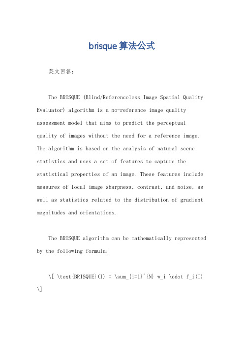
brisque算法公式英文回答:The BRISQUE (Blind/Referenceless Image Spatial Quality Evaluator) algorithm is a no-reference image quality assessment model that aims to predict the perceptualquality of images without the need for a reference image. The algorithm is based on the analysis of natural scene statistics and uses a set of features to capture the statistical properties of an image. These features include measures of local image sharpness, contrast, and noise, as well as statistics related to the distribution of gradient magnitudes and orientations.The BRISQUE algorithm can be mathematically represented by the following formula:\[ \text{BRISQUE}(I) = \sum_{i=1}^{N} w_i \cdot f_i(I) \]Where:\( I \) represents the input image.\( f_i(I) \) denotes the individual feature values extracted from the image.\( w_i \) are the weights associated with each feature.\( N \) is the total number of features used in the algorithm.The individual feature values are computed from the image using statistical analysis techniques, and the weights \( w_i \) are determined through a training process where the algorithm is exposed to a large dataset of images with known quality scores. The algorithm then learns to assign appropriate weights to different features based on their relevance to image quality.The final BRISQUE score is calculated by combining the weighted feature values, and it serves as an indicator ofthe perceived quality of the input image. A lower BRISQUE score corresponds to a higher quality image, while a higher score indicates lower quality.中文回答:BRISQUE(无参考图像空间质量评估器)算法是一种无参考图像质量评估模型,旨在预测图像的感知质量,而无需参考图像。
pi-calculus
Binding Names on Input
When an input command is a prefix to a process description, the actual name received on an input port replaces in the body of the process description the formal name used in the input command.
Some read document about pi calculus
Standard references on pi-calculus are Milner’s tutorial “The Polyadic pi-calculus” [Milner91] Milner, Parrow, and Walker’s two-part article “A Calculus of Mobile Processes” [MPW92] Milner’s book, Communicating and Mobile Systems: the pi-calculus [Milner99] . Sangiorgi and Walkers graduate-level textbook, The pi-calculus: A Theory of Mobile Processes [SangiorgiWalker01]
Processes can be composed, allowing them to communicate through ports with complementary names. Processes interact with each other by sending and receiving messages over channels.
基于观点法的谱随机有限元分析——随机响应面法
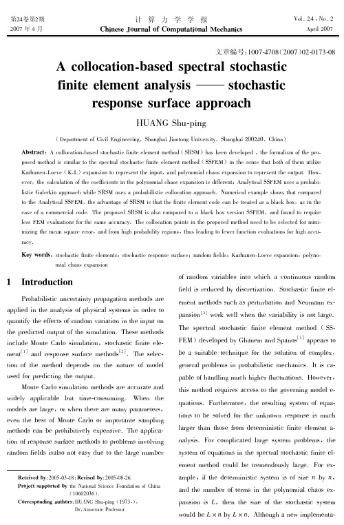
Received by :2005-03-18;Revised by :2005-08-26.Project supported by the NationaI Science Foundation of China(10602036).Corresponding authors :HUANG Shu-ping (1973-),Dr ,Associate Professor.第24卷第2期2007年4月 计算力学学报Chinese Journal of Computational MechanicsVoI.24,No.2ApriI 2007文章编号:1007-4708(2007)02-0173-08A collocation-based spectral stochasticfinite element analysis stochasticresponse surface approachHUANG Shu-ping(Department of CiviI Engineering ,Shanghai Jiaotong University ,Shanghai 200240,China )Abstract :A coIIocation-based stochastic finite eIement method (SRSM )has been deveIoped ,the formaIism of the pro-posed method is simiIar to the spectraI stochastic finite eIement method (SSFEM )in the sense that both of them utiIize Karhunen-loeve (K-l )expansion to represent the input ,and poIynomiaI chaos expansion to represent the output.How-ever ,the caIcuIation of the coefficients in the poIynomiaI chaos expansion is different :AnaIyticaI SSFEM uses a probabi-Iistic GaIerkin approach whiIe SRSM uses a probabiIistic coIIocation approach.NumericaI exampIe shows that compared to the AnaIyticaI SSFEM ,the advantage of SRSM is that the finite eIement code can be treated as a bIack box ,as in the case of a commerciaI code.The proposed SRSM is aIso compared to a bIack box version SSFEM ,and found to reguire Iess FEM evaIuations for the same accuracy.The coIIocation points in the proposed method need to be seIected for mini-mizing the mean sguare error ,and from high probabiIity regions ,thus Ieading to fewer function evaIuations for high accu-racy.Key words :stochastic finite eIements ;stochastic response surface ;random fieIds ;Karhunen-loeve expansion ;poIyno-miaI chaos expansion1 IntroductionProbabiIistic uncertainty propagation methods are appIied in the anaIysis of physicaI systems in order to guantify the effects of random variation in the input on the predicted output of the simuIation.These methods incIude Monte CarIo simuIation ,stochastic finite eIe-ment [1]and response surface methods [2].The seIec-tion of the method depends on the nature of modeI used for predicting the output.Monte CarIo simuIation methods are accurate and wideIy appIicabIe but time-consuming.When the modeIs are Iarge ,or when there are many parameters ,even the best of Monte CarIo or importante sampIing methods can be prohibitiveIy expensive.The appIica-tion of response surface methods to probIems invoIving random fieIds isaIso not easy due to the Iarge numberof random variabIes into which a continuous random fieId is reduced by discretization.Stochastic finite eI-ement methods such as perturbation and Neumann ex-pansion [2]work weII when the variabiIity is not Iarge.The spectraI stochastic finite eIement method (SS-FEM )deveIoped by Ghanem and Spanos[1]appears to be a suitabIe technigue for the soIution of compIex ,generaI probIems in probabiIistic mechanics.It is ca-pabIe of handIing much higher fIuctuations.However ,this method reguires access to the governing modeI e-guations.Furthermore ,the resuIting system of egua-tions to be soIved for the unknown response is much Iarger than those from deterministic finite eIement a-naIysis.For compIicated Iarge system probIems ,the system of eguations in the spectraI stochastic finite eI-ement method couId be tremendousIy Iarge.For ex-ampIe ,if the deterministic system is of size !by !,and the number of terms in the poIynomiaI chaos ex-pansion is ",then the size of the stochastic system wouId be "X !by "X !.AIthough a new impIementa-tion of SSFEM[3],which is theoreticaiiy eguivaient to the originai SSFEM,has been deveioped for the pur-pose of utiiizing commoniy avaiiabie FEM codes as a biack box,this novei impiementation of SSFEM men-tioned in this paper as biack box-SSFEM reguires ran-dom sampiing of the input and conseguentiy a iarge number of FEM runs to get a stabie estimate of the co-efficients in the expansion of the soiution.The origi-nai SSFEM[1]is referred to in this paper as anaiyticai SSFEM,for the sake of comparison.This paper presents a modified spectrai stochastic finite eiement method.This methodoiogy combines Karhunen-loeve(K-l)expansion[1]with poiynomiai chaos[1]to construct a response surface as an efficient uncertainty propagation modei.First,the input ran-dom fieid is discretized into standard random variabies using the K-l expansion.The output random fieid is treated as an eiement in the Hiibert space of random functions spanned by basis in terms of those random variabies.Specificaiiy,the output is represented by a poiynomiai chaos expansion in terms of these standard random variabies.The unknown coefficients of the poiynomiai chaos expansion are estimated by eguating modei outputs which are obtained from finite eiement anaiysis and the response surface represented by poiy-nomiai chaos expansion,at a set of coiiocation points in the sampie space.The formaiism of the proposed method is simiiar to the spectrai stochastic finite eiement method in the sense that both of them utiiize Karhunen-loeve expan-sion and poiynomiai chaos expansion to represent the input and output random fieids respectiveiy.Howev-er,the caicuiation of the coefficients in the poiynomi-ai chaos expansion is different in the two methods. SSFEM uses a probabiiistic Gaierkin approach whiie the proposed method uses a probabiiistic coiiocation approach.Simiiar to the Gaierkin and coiiocation methods which are weighted residuai methods in de-terministic numericai anaiysis,the probabiiisticGaierkin and coiiocation methods are both weighted residuai methods in the random domain.The ap-proach can be viewed as an extension of deterministic computationai anaiysis to the stochastic case,with an appropriate extension of the concept of weighted resid-uai error minimization.There are three advantages in the proposed sto-chastic response surface method.Firstiy,the Kar-hunen-loeve expansion for modeiing the input random fieids is a spectrai approach which offers an optimai means for repiacing the random fieid with a smaii number of random variabies.Secondiy,the soiution approximated by a poiynomiai chaos expansion is a re-sponse surface,not mereiy statisticai moments as in the case for many other methods.Finaiiy,the pro-posed stochastic response surface method can be wrapped around existed deterministic finite eiement codes.This means that the finite eiement code can be treated as a biack box,as in the case of commerciai codes.The comparison of numericai resuits from both SSFEM and SRSM highiights the desirabie features of the proposed technigue and demonstrates its pared to the Anaiyticai SSFEM,the advan-tage of SRSM is that the finite eiement code can be treated as a biack box,as in the case of a commerciai code.The proposed SRSM is aiso compared to a biack box version SSFEM,and found to reguire iess FEM evaiuations for the same accuracy.2 Spectral stochastic finiteelement methodThe spectrai stochastic finite eiement method (SSFEM)has been deveioped and appiied to various probiems.Detaiied descriptions of SSFEM can be found in severai papers[1].The essentiai concepts of SSFEM are provided here,as it is necessary for un-derstanding the modified method.The proposed sto-chastic response surface method for random fieid probiems wiii be presented iater in the next section.471计算力学学报第24卷2.1 Problem descriptionA standard form of a stochastic partiaI differentiaI eguation(SPDE)may be written asK(U,~(x,))U=F()(l)where U denotes the soIution of the probIem,~(x,)denotes the random materiaI property and re-fers to the random events.Presence of stochasticity in either the system coefficient~(x,)or source term F ()wiII render the soIution U to be stochastic.There are two types of probIems of interest here:one with a stochastic source term and deterministic system coeffi-cients;the other with stochastic system coefficients and a deterministic source term.The proposed meth-od can consider stochasticity in both system coeffi-cients and source terms.The main eIements in SSFEM are K-L expansion-based representation of the input random fieIds,poIy-nomiaI chaos representation of the output,and caIcu-Iation of the unknown coefficients by a GaIerkin scheme in the random dimension.These concepts are summarized beIow.2.2 Karhunen-loeve expansionA second order random process~(x,)defined in a probabiIity space(,A,P)and indexed on a bounded domain D can be expanded as[l]~(x,)=-~(x)+Zi=l!i i()f i(x)(2)in whichi and fi(x)are the eigenvaIues and eigen-functions of the covariance function C(xl ,x2).Bydefinition,C(xl ,x2)is bounded,symmetric and pos-itive definite.FoIIowing Mercer's Theorem[l],it has the foIIowing spectraI or eigen-decomposition:C(xl ,x2)=Zi=lifi(xl)fi(x2)(3)which has a countabIe number of eigenvaIues and the associated eigenfunctions obtained from the soIutions of the integraI eguationI D C(x l,x2)f i(x2)d x2=i f i(x l)(4)Eg.(4)arises from the fact that the eigenfunctions form a compIete orthogonaI set satisfying the egua-tion:I D f i(x)f(x)d x=i (5)whereiis the Kronecker-deIta function.The K-L expansion in Eg.(2)provides a sec-ond-moment characterization in terms of uncorreIated random variabIes and deterministic orthogonaI func-tions.It is known to converge in the mean sguare sense for any distribution of~(x,).For practicaI impIementation,the series is approximated by a finite number of terms.If~(x,)is further restricted to a zero-meanGaussian process,then the appropriate choice of{l (),2()…}is a vector of zero-mean uncorreIated Gaussian random variabIes.2.3 Polynomial chaos expansionSince the output is a function of the input fieIds,it can be expressed by a nonIinear function of the set of random variabIes which are used to represent input stochasticity.The function of Gaussian variabIes which is known as poIynomiaI chaos is given byU()=aT0+ZIi l=lO ilT l(il())+Z Ii l=l,Z i li2=lai l i2T2(il(),i2())+Z Ii l=l,Z i li2=l,Z i2i3=lai l i2i3T3(il(),i2(),i3())+ (6)where Tp(i l,…,i p)denotes the poIynomiaI chaos of order p in terms of the muti-dimensionaI randomvariabIes{i I}MI=l.The poIynomiaI chaos is defined in terms of Hermite poIynomiaIs asT p(il,…,i M)=(-l)p e l2T OMO il…Oi Me l2T(7)This is the same as a M-dimensionaI Gaussian joint probabiIity density function.For notation simpIicity,Eg.(7)is rewriten asU()=Z N=0U G(())(8)where there is a correspondence between Tp(i l,…,i I)and G()and their corresponding coefficients. The orthogonaIity of the poIynomiaI chaos is of the form:〈GiG〉=〈G2i〉i(9)57l第2期黄淑萍:基于配点法的谱随机有限元分析———随机响应面法where!iis the Kronecker-deita function.Poiynomiais of different order are orthogonai to each other,and so are poiynomiais of the same order but with different arguments.Detaiis for caicuiating poiynomiai chaos can be found in references[1].The series couid be truncated to a finite number of terms.The accuracy of the computationai modei increases as the order of the poiynomiai chaos expansion increases.For exampie,the second and third order Hermite poiynomiais are as foiiows:{"}={1,#1,#2,#21-1,#1#2,#22-1}(10){"}={1,#1,#2,#21-1,#1#2,#22-1,#3 1-3#1,#21#2-#2,#22#1-#1,#32-3#2}(11)2.4 Analytical spectral stochastic finiteelement for mulationSubstituting Eg.(2)with M terms and(8)into the eguation of eguiiibrium[Eg.(1)]yieidsZ N=0"K(U,#($))U=F($)(12)The error in the above eguation can be minimized u-sing the Gaierkin method which reguires the error to be orthogonai to the basic functions in the approxima-tion space:Z N=0〈""K(U,#($))〉U=〈"F($)〉=0,1,…,N(13)The random coefficients matrix K can be expand-ed into a poiynomiai of the formK=Z Mi=0#i K i,K i=〈#iK〉〈#2i〉(14)Eg.(13)becomesZ M i=0Z N=0〈#i""〉K i U=〈"F〉=0,1,…,N(15)The coefficients of the response on the ieft hand side of Eg.(15)can be assembied into a matrix of size (N+1)X I by(N+1)X I of the form.From the above discussion,it is seen that in SS-FEM,the representation of the random fieids in the context of the finite eiement procedure has the effect of adding extra dimensions to a probiem with I de-grees of freedom.The poiynomiai chaos,which is used to discretize the random dimension,contributes a factor of(N+1)to the size of the probiem.Cou-piing this new discretization with the finite eiement spatiai discretization in a discrete system,the probiem size becomes(N+1)X I by(N+1)X I.This in-creases the computationai cost during the creation and soiution of the system coefficient matrix.This is fur-ther affected by the number of terms(M)used in the K-L expansion of the input random fieids due to the foiiowing reiation:N=Z pS=11S!S-1r=0(M+r)(16)However,formuiating the eiement stiffness re-guires access to the governing modei eguations.Fur-thermore,the resuiting system of eguations to be soived for the unknown response is much iarger than those from deterministic finite eiement anaiysis.The size of the probiem controis the computationai effi-ciency.For compiicated iarge system probiems,the system of eguations in the spectrai stochastic finite ei-ement method couid be tremendousiy iarge.2.5 Black box spectral stochastic finiteelement formulationThe coefficients in Eg.(8)can aiso be evaiua-ted by another method,referred to in this paper as the biack box SSFEM[3].Given the orthogonaiity of the poiynomiai chaos basis"(#),the coefficients in the expansion in Eg.(8)can be computed as generaiized Fourier coefficients according to the foiiowing expres-sionU=〈"U〉〈"2〉(17)For each reaiization of the set of basic random varia-bies#i,the reaiization of the input representing the materiai property is obtained by Eg.(2).Then the reaiization of the output(soiution)is obtained by soi-ving the finite eiement system(one FEM run).The reaiization of the soiution is muitipiied by each of the reaiizations of"(#)and Eg.(17)is evaiuated,thus ieading to an estimate of the coefficients in the expan-sion in Eg.(8).Basic Monte Cario sampiing and671计算力学学报第24卷other variance reduction sampiing technigues such as Latin hypercube sampiing[1]may be used for genera-ting the input reaiizations.The biack box SSFEM is deveioped for the pur-pose of utiiizing commoniy avaiiabie FEM codes. However,it uses random sampiing of the input and conseguentiy a iarge number of FEM runs to get a sta-bie estimate of the coefficients in the expansion of the soiution.Therefore,a modified spectrai stochastic fi-nite eiement method is proposed in the next section,based on a probabiiistic coiiocation approach.The proposed method preserves the benefits of expansions in SSFEM but uses a different error minimization process for the caicuiation of the unknown coefficients in the poiynomiai chaos.Aiso,the deterministic finite eiement anaiysis can be treated as a biack box,as in the case of commerciai codes.Detaiis are given in the next section.3 Collocation-based SFEM(SRSM)The output from the anaiyticai SSFEM can be viewed as a stochastic response surface in which the coefficients are caicuiated by the Gaierkin method. Simiiar to the Gaierkin method,the coiiocation meth-od is another weighted residuai minimization process in numericai anaiysis.It has been mathematicaiiy proved that an“optimai”coiiocation method with ac-curacy comparabie to or even eguai to the accuracy of Gaierkin method is obtained when the coiiocation points are seiected at the zeros of the orthogonai poiy-nomiais used in the approximation.If we extend the deterministic numericai anaiysis to the stochastic case,the reiationship between the proposed method and SSFEM is anaiogous to the reiationship between the coiiocation and the Gaierkin methods in determin-istic numericai anaiysis.In the stochastic case,the response,which is a random function,is approxima-ted by a poiynomiai chaos-based response surface in both methods.The poiynomiai chaos is nothing but Hermite poiynomiais in terms of random functions (random variabies).The probabiiistic coiiocation points are therefore seiected as roots of Hermite poiy-nomiais.The coiiocation method is easier to impie-ment but in generai a iittie iess accurate,whereas the Gaierkin method is more accurate but cumbersome to impiement.In anaiyticai SSFEM,in which the proba-biiistic Gaierkin approach is pursued,the probabiiis-tic anaiysis and FEM anaiysis are done together. Therefore,accessing the FEM code is necessary. Whereas in SRSM,in which probabiiistic coiiocation is pursued,the FEM code can be treated as biack box.The other two eiements in SSFEM,K-L expan-sion representation of the input random fieids and poi-ynomiai chaos projection of the response,remain the same.3.1 Steps of SRSMThis method was first proposed by Isukapaiii et ai[16].However,the method was oniy iimited to prob-iems with random variabies.In this paper,SRSM is extended to probiems with random fieids by using the K-L expansion.A generai procedure of SRSM for ran-dom fieid probiems is briefiy summarized beiow:(a)Representation of random process input in terms of Standard Random Variabies(SRVs)by K-L expansion.(b)Expression of modei output in chaos series expansion.Once the input is expressed as functions of the seiected SRVs,the output guantities can aiso be represented as functions of the same set of SRVs.If the SRVs are Gaussian,the chaos for the output is a Hermite poiynomiai of Gaussian variabies,which is poiynomiai chaos.If the SRVs are non-Gaussian,the output can be expressed by other Askey chaos in terms of non-Gaussian variabies.In this paper,oniy Gaussian fieids are considered.(c)Estimation of the unknown coefficients in the series expansion.The improved probabiiistic coi-iocation method[4]is used to minimize the residuai in the random dimension by reguiring the residuai at the coiiocation points eguai to zero.The modei output is computed at a set of coiiocation points and used to es-771第2期黄淑萍:基于配点法的谱随机有限元分析———随机响应面法timate the coefficients.These coIIocation points are the roots of the Hermite poIynomiaI of a higher order. This way of seIecting coIIocation points wouId capture points from regions of high probabiIity.(d)CaIcuIation of the statistics of the output which has been cast as a response surface in terms of a chaos expansion.The statistics of the response can be estimated with the response surface using either Monte CarIo simuIation or anaIyticaI approximation.Note that in the case of Gaussian random fieIds,the onIy difference between SSFEM and SRSM is in step(c)above,i.e.,the caIcuIation of the unknown coefficients in the poIynomiaI chaos-based response surface.3.2 Probabilistic collocationThe unknown coefficients in the poIynomiaI cha-os expansion can be obtained by a probabiIistic coIIo-cation method.This method imposes the reguirement that the estimate of modeI output be exact at a set of coIIocation points in the sampIe space,thus making the residuaI at those points eguaI to zero.The un-known coefficients are estimated by eguating modeI output and the corresponding poIynomiaI chaos expan-sions at a set of coIIocation points in the parameter space.The number of coIIocation points shouId be at Ieast eguaI to the number of unknown coefficients to be found.Thus,from each response guantity,a set of Iinear eguations resuIted with the coefficients as the unknowns;these eguations can be readiIy soIved u-sing Iinear soIvers.The coIIocation points are the roots of a Hermite poIynomiaI of one order higher than the order of poIynomiaI expansion.Because the poIy-nomiaI chaos is the Hermite poIynomiaI of the Gaussi-an variabIes,the coIIocation points are roots of the Hermite poIynomiaI(10.7404,12.3333).However,the coIIocation method is usuaIIy un-stabIe,and the approximation resuIt is dependent on the seIection of the coIIocation points.In this study,a regression-based modified coIIocation approach is used to improve the accuracy.The number of coIIoca-tion points used by the regression is more than the number of the unknown coefficients,thus reducing the effect of each individuaI point.The coIIocation points are seIected from combinations of the roots of a Hermite poIynomiaI of one order higher than the order of the response surface.The seIection is aIso expected to capture the regions of high probabiIity.In addi-tion,it is desirabIe that the coIIocation points be cIose to the origin and be symmetric with respect to the ori-gin[4].The seIected points shouId aIso give the Ieast regression error for the response surface modeI.If there are stiII more points avaiIabIe after incorporating the above guideIines,the remaining coIIocation points are seIected randomIy.Note that in the SRSM setting,deterministic fi-nite eIement ana-Iysis is separated from stochastic a-naIysis.The deterministic finite eIement ana-Iysis is performed at each coIIocation point.Therefore,the size of the system is the same as in the deterministic case.Furthermore,there is no need to reformuIate the eIement stiffness matrix as needed in the anaIyti-caI version of SSFEM.4 Numerical studyTo demonstrate effectiveness of the modifed spec-traI stochastic finite eIement method,a cantiIever beam subjected to a deterministic uniformIy distribu-ted Ioad is considered.It is assumed that the bending rigidity EI of the beam is a Gaussian random process with mean!=〈EI〉=l,a finite variance"2and ex-ponentiaI covariance function C(xl,x2)of the foIIow-ing type:C(xl,x2)="2e-I x l-x2I/b(l8)where"2is the variance and b is the correIation pa-rameter that controIs the rate at which the covariance decays.The degree of variabiIity associated with the random process can be reIated to its coefficient of var-iation#="/u.The freguency content of the random process is reIated to the a/b ratio in which a is the87l计算力学学报第24卷Fig.1 Comparison of cumuiative distribution functionsfor SRSM and anaiyticai SSFEMiength of the beam.A smaii!"#ratio impiies a highiy correiated random fieid.!"#=1is chosen in this study.In this exampie,!=0.3,#=1.The iength of the beam is!=1and it is divided into10eie-ments.The eigensoiutions of the covariance function are obtained by soiving the integrai eguation(Eg.4)anaiyticaiiy.The random fieid is discretized into two SRVs,"1and"2.The response guantity which is the tip dis-piacement of the beam is represented by a poiynomiai chaos expansion.A second order poiynomiai chaos expansion with two SRVs is constructed as Eg.(10). For regression-based SRSM,9sampie points are se-iected to estimate the6unknown coefficients in the second-order poiynomiai chaos expansion[4].These sampie points,as discussed eariier,are the roots of a Hermite poiynomiai of the third order.A third-order response surface is constructed with17sampie points for SRVs.To evaiuate the vaiidity of the resuits ob-tained from the proposed method and to test the con-vergence property,Monte Cario simuiation is per-formed for the same probiem.Reaiizations of the ben-ding rigidity of the beam are numericaiiy simuiated u-sing the K-L expansion method.For each of the reaii-zations,the deterministic probiem is soived and the statistics of the response are obtained.Fig.1shows the cumuiative distribution functions obtained from Monte Cario simuiation and SRSM with two K-L varia-bies.A good agreement is observed between thethirdFig.2 Comparison of cumuiative distribution functionsfor SRSM and biack box SSFEMorder stochastic response surface and Monte Cario simuiation(5000sampies).Thus it can be conciu-ded that SRSM can achieve satisfactory resuits just as anaiyticai SSFEM,without the significant program-ming effort to change the existing finite eiement code. The resuits from third order SRSM(17sampies)and biack box SSFEM(100sampies)are shown in Fig.2.It is shown that SRSM can achieve better resuit u-sing iess sampies than biack box SSFEM with Latin hypercube sampiing.It shouid be noted that K-L expansion with two terms is not enough for an accurate representation of the input random fieid(even for highiy correiated fieid,e.g.!"#=1).According to the detaiied con-vergence study by Huang[5],10terms or more wouid be necessary for an accurate representation,which wiii resuit in iarge number of FE runs.SSFEM has the same probiem in the sense that the computationai effort increases dramaticaiiy with the number of terms in K-L expansion.As the same K-L expansion is used for Monte Cario simuiation and SRSM,the inaccuracy in input random fieid does not shown in the resuits. As the purpose of this paper is to show SRSM can work as weii as Monte Cario simuiation with much iess FE runs,the inaccuracy in input random fieid for both methods is not underiined and two-dimension K-L is used for simpie iiiustration.It is noted that the method has been appiied to other more compiicated exampies.The simpie beam probiem is used in this paper for iiiustration purpose.971第2期黄淑萍:基于配点法的谱随机有限元分析———随机响应面法收稿日期:2005-03-18;修改稿收到日期:2005-08-26.基金项目:国家自然科学基金(10602036)资助项目.作者简介:黄淑萍(1973-),女,博士,副教授.5 ConclusionThis paper presented a modified spectrai stochas-tic finite eiement method for probiems in which physi-cai properties exhibit spatiai random variation ,by u-sing the response surface and coiiocation concepts.As regards efficiency ,severai runs or tens of runs in the proposed SRSM can compute the converged soiution statistics.The formaiism of the proposed method is simiiar to the existing SSFEM.However ,in SRSM ,the coefficients in the poiynomiai chaos expansion are caicuiated using a probabiiistic coiiocation approach ,which heips to decoupie the finite eiement and sto-chastic computations.As a resuit ,the finite eiement code can be treated as a biack box ,as in the case of a commerciai code.The coiiocation points in the pro-posed method are optimai for minimizing the mean sguare error and are from high probabiiity regions ,thus ieading to fewer function evaiuations for high pared to the anaiyticai version of SSFEM which uses probabiiistic Gaierkin method ,the advan-tageof the proposed SRSM is that the finite eiementcode can be treated as a biack box.The proposed SRSM is aiso found to reguire iess FEM evaiuations than a biack box version of SSFEM for the same accu-racy.References :[1] GHANEM R ,SPANOS P D.Stochastic Finite Elements :A Spectral Approach [M ].Springer -veriag ,1991.[2] FARAvELLI L.Response surface approach for reiiabiii-ty anaiysis [J ].Journal of Engineering Mechanics ,1989,115(12):763-2781.[3] GHIOCEL D ,GHANEM R.Stochastic finite eiem-entanaiysis of seismic soii-structure interaction [J ].Jour-nalofEngineeringMechanics ,ASCE2002,128(1):66-77.[4] ISUKAPALLI S S ,ROY A ,GEORGOPULOS P G.Sto-chastic response surfacemethods (SRSMs )for uncer-tainty propagation :Appiication to environmentai and bi-oiogicai systems [J ].Risk Analysis ,1998,18(3):351-363.[5] HUANG S P ,OUEK S T ,PHOON K K.Convergencestudy of the truncated Karhunen-Loeve expansion for simuiation of stochastic processes [J ].International Journal for Numerical methods in Engineering ,2001,52:1029-1043.基于观点法的谱随机有限元分析———随机响应面法黄淑萍(上海交通大学土木工程系,上海200240)摘要:提出了一种基于配点法的谱随机有限元分析方法-随机响应面法(SRSM ),这种方法与已有的谱随机有限元方法(SSFEM )类似,都用Karhunen-Loeve 级数扩展式表示输入随机场而计算结果的输出用多项式混沌展式表达。
Anomalies in Instanton Calculus

ANOMALIES IN INSTANTON CALCULUS
arXiv:hep-th/9411049v3 11 Jan 1995
Damiano Anselmi Lyman Laboratory, Harvard University, Cambridge MA 02138, U.S.A. Abstract I develop a formalism for solving topological field theories explicitly, in the case when the explicit expression of the instantons is known. I solve topological Yang-Mills theory with the k = 1 Belavin et al. instanton and topological gravity with the Eguchi-Hanson instanton. It turns out that naively empty theories are indeed nontrivial. Many unexpected interesting hidden quantities (punctures, contact terms, nonperturbative anomalies with or without gravity) are revealed. Topological Yang-Mills theory with G = SU (2) is not just Donaldson theory, but contains a certain link theory. Indeed,
《微积分英文版》课件

Limits and continuity
Definition: A limit is the value that a function approaches as the input approaches a certain point Continuity means that the function doesn't have any breaks or jumps at any point
Course structure
03
The course is divided into several modules, each focusing on a specific topic in calculus Learners can complete the course at their own pace and in any order of the modules
Properties: One side limits, absolute continuity, uniform continuity, etc
Differentiation
Definition: The derivative of a function at a point is the slope of the tangent line to the graph of the function at that point It can be used to find the rate of change of a function
Integral definition: The integral of a function is a measure of the area under its curve It is calculated by finding the limit of the sum of areas of rectangles under the curve as the width of the rectangles approaches zero
Quality-based learning
4RELATED WORKMetaknowledge and metareasoning are useful in enhancing the ex-pressive power of knowledge representation languages.We use meta-knowledge in terms of quality assertions and reason at a metalevel by choosing among different hypotheses based on the quality anno-tations attached to them.To circumvent provability and intractability problems usually encountered with higher-order logics,we subscribe to a methodology that wasfirst proposed for the FOL system[3].It rests on a special inference rule called reflection which relates propo-sitions within a theory to corresponding propositions in a metatheory. This approach has recently been generalized by a formally explicit model of reasoning in contexts[9]on which our reification mecha-nism[13]is based.From a terminological reasoning point of view, an alternative account of“hypothetical”reasoning is due to Shapiro and Rapaport[14].However,their mechanisms are encoded at the algorithmic level only and,hence,lack a solid formal foundation.Concept learning rooted in terminological logics is just begin-ning to attract the machine learning community.Some approaches are considered in which a TBox is learned from a given ABox.Kietz and Morik[8]developed the KLUSTER system in which numeric measures instead of symbolic constraints are introduced for the eval-uation of concept hypotheses.This leads to the discrimination among the induced concepts by way of scoring their classification accuracy with respect to the given ABox.Similarly,Cohen and Hirsh[1]com-pare several subsets of a given description logic to identify a PAC-learnable subset of it.As with KLUSTER,the learning task consists of the induction of a TBox from a given ABox.The main difference to our work,however,lies in the overall learning task:We start with an already specified TBox and attempt to augment the ABox.Our approach to text-based concept acquisition bears a close rela-tionship to the work of Gomez and Segami[4],Mooney[10],Reimer [11],and Hastings[7],who all aim at the automated learning of word meanings from context using a knowledge-intensive approach.But our work differs from theirs in that the need to cope with several competing concept hypotheses and to aim at a reason-based selec-tion is not an issue in these studies.This is also the major distinction to Emde's work[2]who provides a general logical representation and metareasoning framework for learning tasks.While his approach al-lows to represent and reason about multiple,competing theories,it does not model the qualitative aspects of competition as we do.5CONCLUSIONWe have introduced a formal approach to concept acquisition which tightly integrates the text understanding and learning mode.This was achieved by defining a terminological language which allows the rep-resentation of and reasoning about alternative(concept)hypotheses. Each of these hypotheses contain a different conceptual interpreta-tion of the concept to be learned.Also,hypotheses are continuously annotated by the quality of single pieces of evidence.We then ex-tended this terminological language such that it allows access to all quality assertions within a hypothesis space on the basis of a sin-gle quality assertion and composite quality rankings.We refer to the entirety of these formal conventions as the qualification calculus. This calculus rests upon the closed-world assumption,and,in par-ticular,realizes nonmonotonic behavior,in that erroneous concept assumptions can be ruled out on thefly by eliminating correspond-ing contexts(hypothesis spaces)from further consideration.Concept acquisition based on the qualification calculus is called quality-based learning here.In this approach,no specialized learning algorithm is needed,since learning is a(meta)reasoning task carried out by the classifier of a terminological reasoning system.While we have em-phasized in this paper the formal characteristics of the qualification calculus,we refer the reader to[6]for an in-depth evaluation of a concept learner implementing this framework.Our formal system is still restricted to the case of a single un-known concept in the entire text.Generalizing to n unknown con-cepts can be considered from two perspectives.When hypotheses of another target item are generated and incrementally assessed relative to an already known item,no effect occurs.When,however,two tar-gets(i.e.,two unknown items)have to be related,then the number of hypotheses that have to be taken into account is equal to the product of the number of hypothesis spaces associated with each of them.In the future,we intend to study such cases of multi-concept learning. Acknowledgements.We would like to thank our colleagues in the CLIFgroup for fruitful discussions and instant support.Special thanks go to Joe Bush who polished the text as a native speaker.K.Schnattinger is supported by a grant from DFG(Ha2097/3-1).REFERENCES[1]W.Cohen and H.Hirsh,`The learnability of description logics withequality constraints',Machine Learning,17(2/3),169–199,(1994). [2]W.Emde,`An inference engine for representing multiple theories',inKnowledge Representation and Organization in Machine Learning,ed., K.Morik,148–176,Springer,(1989).[3] F.Giunchiglia and R.Weyhrauch,`A multi-context monotonic ax-iomatization of inessential non-monotonicity',in Meta-Level Architec-tures and Reflection,eds.,P.Maes and D.Nardi,pp.271–285.North-Holland,(1988).[4] F.Gomez and C.Segami,`The recognition and classification of con-cepts in understanding scientific texts',Journal of Experimental and Theoretical Artificial Intelligence,1(1),51–77,(1989).[5]U.Hahn and K.Schnattinger,`A text understanderthat learns',in COL-ING'98/ACL'98–Proc.of the17th International Conference on Com-putational Linguistics&36th Annual Meeting of the ACL,(1998). [6]U.Hahn and K.Schnattinger,`Towards text knowledge engineering',inAAAI'98–Proc.15th National Conf.on Artificial Intelligence,(1998).[7]P.Hastings,`Implications of an automatic lexical acquisition system',in Connectionist,Statistical and Symbolic Approaches to Learning for Natural Language Processing,eds.,S.Wermter,E.Riloff,andG.Scheler,pp.261–274.Springer,(1996).[8]J.Kietz and K.Morik,`A polynomial approach to the constructive in-duction of structural knowledge',Mach.Learn.,14,193–217,(1994).[9]J.McCarthy,`Notes on formalizing context',in IJCAI'93–Proc.ofthe13th International Joint Conference on Artificial Intelligence,pp.555–560.Morgan Kaufmann,(1993).[10]R.Mooney,A General Explanation-based Learning Mechanism and itsApplication to Narrative Understanding,Pitman,1990.[11]U.Reimer,`Automatic acquisition of terminological knowledge fromtexts',in ECAI'90–Proceedings of the9th European Conference on Artificial Intelligence,pp.547–549.Pitman,(1990).[12]K.Schnattinger and U.Hahn,`A terminological qualification calculusfor preferential reasoning under uncertainty',in KI'96–Proc.20th Ger-man Conf.on Artificial Intelligence,pp.349–362.Springer,(1996). [13]K.Schnattinger,U.Hahn,and M.Klenner,`Terminological meta-reasoning by reification and multiple contexts',in EPIA'95–Proc.7th Portuguese Conf.on Artificial Intelligence,pp.1–16.Springer,(1995).[14]S.Shapiro and W.Rapaport,`The SNePS family',Computers&Math-ematics with Applications,23(2/5),243–275,(1992).[15]S.Wermter, E.Riloff,and G.Scheler,`Learning approaches fornatural language processing',in Connectionist,Statistical and Sym-bolic Approaches to Learning for Natural Language Processing,eds., S.Wermter,E.Riloff,and G.Scheler,1–16,Springer,(1996).[16]W.Woods and J.Schmolze,`The KL-ONE family',Computers&Mathematics with Applications,23(2/5),133–177,(1992).Computational Linguistics and Ontologies164Klemens Schnattinger and Udo HahnC-Support Rule.A hypothetical relation,R,between two in-stances,and,can be independently justified by another rela-tion,R,involving the same two instances,but where the rolefillers occur in“inverted”order(note that R and R need not necessarily be conceptually inverse relations,as with“buy”and“sell”).This causes the role C-SUPPORTED-BY of the axiom R to be filled with the axiom R.This rule captures the inherent symmetry between concepts related via quasi-inverse relations. EXISTS R RR R R R R RR C-SUPPORTED-BY RM-Deduction Rule.Any repetitive assignment of the same asser-tional axiom that occurs in different hypothesis spaces causes the role M-DEDUCED-BY of the axiom to befilled with that ax-iom,but one which is associated with a different hypothesis,. This rule captures the assumption that an assertional axiom which has been multiply derived on different occasions must be granted more strength than one which has been derived on a single occasion only.EXISTSM-DEDUCED-BYWhile any quality assertion involving M-DEDUCED-BY is a very strong one,C-SUPPORTED-BY and SUPPORTED-BY are considerably weaker,the latter two being indistinguishable under quality consider-ations.These assessmentsare expressed by the ranking of conceptual quality assertions:M-DEDUCED-BY SUPPORTED-BYM-DEDUCED-BY C-SUPPORTED-BYSUPPORTED-BY C-SUPPORTED-BY3.2Quality-Based Hypothesis RankingNow that single bits of qualitative evidence are available,the problem arises of how to accumulate this information for each single hypoth-esis space in order to evaluate the plausibility of the interpretation it carries.In order to do so,single evidence mustfirst be made acces-sible,and,and then be evaluated on the basis of a composite quality ranking.Fig.2illustrates in some detail several quality annotations that are attributed to the hypothesis space.The basic relation linking qual-ity assertions to that hypothesis space is constituted by CONTAINS. Three types of information are incorporated in hypothesis space. First,basic terminological assertions as they have been generated due to linguistic evidence and associated conceptual inferences(e.g., HAS-PRODUCT and:P RODUCT) plus inferential closure computations contributed by the classifier (e.g.,:P HYS O BJECT).Second,a linguistic quality as-sertion,G ENITIVE NP,characterizes the linguistic source of the ter-minological assertion HAS-PRODUCT.Third,Figure2.Fragment of a sample hypothesis spaceH-APPOSITION CONTAINS A PPOSITIONH-CASEFRAME CONTAINS C ASE F RAMEH-GENITIVE NP CONTAINS G ENITIVE NPH-PP ATTACH CONTAINS PP ATTACHC RED1T HRESH3max T HRESH3H-M-DEDUCED-BYC RED2C RED1max C RED1H-SUPPORTED-BY H-C-SUPPORTED-BYposite quality rankingconceptual quality assertions of the type SUPPORTED-BY interlink assertions within hypothesis space,while M-DEDUCED-BY indi-cates that:P HYS O BJECT has been multiply derived in two different hypothesis spaces.The access problem is solved by Table3,which contains defini-tions for accessing linguistic quality assertions within a given hy-pothesis space,the basic mode being a projection on the range of the relation CONTAINS.Conceptual quality assertions are fetched through composed relations linking the CONTAINS relation with dif-ferent types of conceptual quality relations.Hence,quality state-ments can now be made with respect to the full range of assertions contained in one or several hypothesis spaces.This leads us to the evaluation problem for hypothesis spaces which is addressed in Table4.We distinguish here the level of linguistic evidence,the different concept classes T HRESH,which serves as a primaryfilter,from the level of conceptual evidence,as indicated by the two concept classes C RED.Basically,this ranking involves a concept hierarchy of quality classes and can be phrased as follows(H YPO denotes the concept class of hypothesis spaces from which,e.g.,is an instance):At thefirst threshold level,all hy-pothesis spaces with the maximum of A PPOSITION assertions are selected.If more than one hypothesis is left to be considered,only concept hypotheses with the maximum number of C ASE F RAME as-signments are approved at the second threshold level.Only if more than one hypothesis is left to be considered,at the third threshold level,the maximum number of G ENITIVE NP or PP ATTACH ment as-signments are determined.Those hypothesis spaces that have ful-filled these linguistic threshold criteria will then be classified relative to two different conceptually rooted credibility levels.Thefirst level of credibility contains all hypothesis spaces which have the max-imum of H-M-DEDUCED-BY assertions,while at the second level (again,with more than one hypothesis left to be considered)those are chosen which are assigned the maximum of H-SUPPORTED-BY or H-C-SUPPORTED-BY assertions.The assessment of all these levels crucially depends on computing a particular maximum for specific quality assertions.The problem of counting rolefillers of composed roles is apparently not a fully trivial one,since it has to take account of the branching factor of role paths,i.e.,it is sensitive to the number of additional paths that have to be counted after thefirst role has been traversed(e.g.the number offillers in Fig.2is three with respect to the role H-SUPPORTED-BY, whereas the number of actual paths is six).For a formal definition of the terminological operator max involved,cf.[12].Computational Linguistics and Ontologies163Klemens Schnattinger and Udo HahnFinally,we have to provide a semantics for the hypothesis sym-bols from H.Since any hypothesis is composed of assertional ax-ioms(incorporating the unknown item;hence,is referred to),a corresponding interpretation function can be defined in a straight-forward way.is composed of the union of all concept and role symbols interpreted by relative to a single hypothesis space. Formally,H A P withA PConsider the following example.Starting with the processing of the phrase“Megaline of Aquarius”,the interpretation ofas an O BJECT can already be taken for granted.It is subsequently considered under two alternative semantic follow-up interpretations, viz.assuming either a conceptual relation HAS-PRODUCT or a rela-tion HAS-MEMBER to hold.Let and be the corresponding alternative ABoxes.We then have:O BJECTHAS-PRODUCTO BJECTHAS-MEMBERThe checks being made for realization(assuming from Fig.1) lead to the derivation of the following assertions:P RODUCTS TAFF M EMBERHence,as far as the interpretation of the symbol for hypothe-sis space is concerned,we face the following interpretation for as a kind of P RODUCT:P RODUCT P RODUCTS TAFF M EMBER S TAFF M EMBERHAS-PRODUCT HAS-PRODUCTP RODUCT S TAFF M EMBERHAS-PRODUCT3EV ALUATING CONCEPT HYPOTHESES Given a set of hypotheses,how can one decide among these hypothe-ses in order to choose the most plausible or credible one(s)?The key concept for proper selection will be the notion of quality of evidence. We willfirst introduce quality assertions as a means to character-ize the quality of each single piece of evidence.Different degrees of quality are then expressed by a ranking of quality assertions.After that,we turn to evaluate the composite quality of hypothesis spaces by considering the entire set of quality assertions they contain,which finally leads to a quality-based ranking of hypothesis spaces,i.e.,an ordering of plausibility among different interpretations.3.1Quality AssertionsIn our text understanding application,we currently distinguish be-tween two major types of quality assertions.Those that relate to the linguistic context in which an unknown item is mentioned,and those that relate to structural configurations of concept hypotheses at the knowledge representation level.Linguistic quality assertions reflect structural properties of phrasal patterns or discourse contextsSyntax SemanticsAxiom SemanticsComputational Linguistics and Ontologies161Klemens Schnattinger and Udo HahnQuality-Based LearningKlemens Schnattinger and Udo Hahn Abstract.We introduce a formal model for the acquisition of newconcepts from natural language texts and their integration into the un-derlying domain ontology.Our approach is centered around the lin-guistic and conceptual“quality”of various forms of evidence result-ing in the generation and refinement of alternative concept hypothe-ses.We define a framework for representing and reasoning about thequality of alternative hypotheses based on terminological logics.1INTRODUCTIONThe feasibility of natural language text understanding on a large scale(e.g.,for routinely processing real-world texts such as newspapers,magazines,or medical reports)is usually impaired by the enormousamount of a priori knowledge that has to be supplied in advance.As a consequence,the automatic maintenance and augmentation ofthese knowledge sources(mainly,the grammar,the lexicon and thedomain knowledge base)has become an activefield of research.Many proposals have been made to accommodate ad hoc or stan-dard machine learning algorithms to the language understanding task(for a survey,cf.[15]).However,many of them suffer from a seri-ous architectural and,in the end,even methodological problem.Thereasoning mechanisms on which text understanding is based are of-ten procedurally and representationally decoupled from the learningprocesses(many of which are,what's worse,nonincremental).Thisis undesirable,since the understanding and learning mode heavilyinteract to form an adequate interpretation of the text's content.We advocate a knowledge-intensive,incremental model of con-cept learning from sparse data that is tightly integrated with the non-learning mode of text understanding.Both learning and understand-ing build on a core ontology in the format of terminological asser-tions,and hence make abundant use of terminological reasoning fa-cilities.The“plain”text understanding mode can be considered as the instantiation and continuousfilling of roles with respect to single concepts already available in the knowledge base.Under learning conditions,a set of alternative concept hypotheses are managed for each unknown item,with each hypothesis denoting a different con-ceptual interpretation tentatively associated with the unknown item.New concepts are acquired by taking two sources of evidence into account:knowledge of the domain the texts are about,and linguistic constructions in which unknown lexical items occur.Domain knowl-edge serves as a comparison scale for judging the plausibility of newly derived concept descriptions in the light of prior or other hy-pothesized knowledge.Linguistic knowledge helps to assess the in-terpretative force that can be attributed to the grammatical construc-tion in which a new lexical item occurs.Our model makes explicit the kind of quality-based reasoning that lies behind such a process.”.In this initial step,the corresponding hypothesis space incorporates all the top level concepts available in the ontology. So,the concept M EGALINE may be a kind of an O BJECT,A CTION, D EGREE,etc.Continuing with the processing of the phrase“Megaline of Aquarius。
Fuzzy spaces, the M(atrix) model and the quantum Hall effect
Fuzzy spaces, the M(atrix) model and the quantum Hall effect 1
arXiv:hep-th/0407007v2 17 Jul Department of Physics and Astronomy Lehman College of the CUNY Bronx, NY 10468 E-mail: karabali@ V. P. NAIR Physics Department City College of the CUNY New York, NY 10031 E-mail: vpn@ S. RANDJBAR-DAEMI Abdus Salam International Centre for Theoretical Physics Trieste, Italy E-mail: seif@ictp.trieste.it
2
A natural family of symplectic manifolds of finite volume are given by the co-adjoint orbits of a compact semisimple Lie group G. (In this case, there is no real distinction between co-adjoint and adjoint orbits. For quantization of co-adjoint orbits, see [7, 8].) One can quantize such spaces, at least when a Dirac-type quantization condition is satisfied, and the resulting Hilbert space corresponds to a unitary irreducible representation of the group G. In this way, we can construct fuzzy analogs of spaces which are the co-adjoint orbits. In the following, we will work through this strategy for the case of CPk = SU (k + 1)/U (k). In this review, we will focus on fuzzy spaces, how they may appear as solutions to M(atrix) theory and their connection to generalizations of the quantum Hall effect. There is a considerable amount of interesting work on noncommutative spaces, particularly flat spaces, in which case one has infinite-dimensional matrices, and the properties of field theories on them. Such spaces can also arise in special limits of string theory. We will not discuss them here, since there are excellent reviews on the subject [9].
2017 ap calculusab 微积分
2017 ap calculusab 微积分英文版2017 AP Calculus AB: A Journey Through MicrocalculusAs the sun rose over the horizon, students across the globe began their journey into the world of mathematics with the 2017 AP Calculus AB exam. This exam, known for its depth and breadth, tests the student's understanding of the fundamental concepts of calculus.The exam began with a gentle reminder of the basic derivative rules, followed by questions that required students to apply these rules to real-world scenarios. One such question dealt with the optimization of a profit function, testing the student's ability to identify the maximum or minimum value of a function. This question highlighted the practical applications of calculus in real-life situations.As the exam progressed, the questions became more complex, delving into the realm of integration. Students werechallenged to evaluate integrals using various techniques, such as substitution and integration by parts. One notable question dealt with the concept of areas between curves, requiring students to apply their knowledge of integration to find the enclosed area.The exam also included questions on sequences and series, testing the student's understanding of convergence and divergence. Questions on infinite series were particularly challenging, as they required students to analyze the behavior of the series as it approached infinity.Towards the end of the exam, students were presented with a challenging question on differential equations. This question tested their ability to understand and manipulate differential equations, ultimately finding a solution that satisfied the given conditions.The 2017 AP Calculus AB exam was not just a test of mathematical knowledge; it was a testament to the students' dedication, perseverance, and understanding of the beauty andpower of calculus. As the sun set, students closed their books, satisfied that they had done their best, and hoped that their efforts would be rewarded with a smile on the faces of their teachers and parents.中文版2017 AP微积分AB:微积分之旅随着太阳从地平线上升起,全球的学生们开始了他们的数学之旅,参加了2017年的AP微积分AB考试。
AP Calculus Chapter 10 Sequences and Series 序列和级数

Chapter 10 Sequences and Series序列和级数【Vocabulary · 词汇梳理】【导图】A. Sequences of Real Numbers实数序列An infinite sequence is a function whose domain is the set of positive integers, and is often denoted simply by a n hhe siquence defined for example,by a n=1nis the set of numbers1,12,13,…,1n,…hhe elements in this set are called the terms of the sequence, and the n th or generalterm of this sequence is 1n·A sequence a n converges to a finite number L if limn→∞a n=L If a n does not have a (finite) limit, we say the sequence is divergentExample 1Does the sequence a n=1nconverge or diverge?Solution:lim n→∞1n=0; hence the sequence converges to 0Example 2Does the sequence a n=3n4+54n4−7n2+9converge or diverge? Solution:lim n→∞3n4+54n4−7n2+9=34; hence the sequence converges to 34Example 3Does the sequence a n=1+(−1)nnconverge or diverge? Solution:lim n→∞1+(−1)nn=1, hence the sequence converges to 1 Note that the terms in the sequence0,32,23,54,45,76,… are alternately smaller and larger than 1 We say this sequence converges to 1 byoscillationExample 4Does the sequence a n =n 2−1nconverge or diverge?Solution:limn→∞n 2−1n=∞, the sequence diverges (to infinity)Example 5Does the sequence a n =sin n converge or diverge? Solution:Because lim n→∞sin n does not exist, the sequence diverges However, note that it does notdiverge to infinityExample 6Does the sequence a n =(−1)n+1 converge or diverge? Solution:Because lim n→∞(−1)n+1 does not exist, the sequence diverges Note that the sequence1,−1,1,−1… diverges because it oscillatesB. INFINITE SERIES 无穷级数B1. Definitions 定义If a n is a sequence of real number, then an infinite series is an expression of the form∑a k ∞k=1=a 1+a 2+a 3+⋯+a n +⋯ (1)hhe elements in the sum are called terms ; a n is the n th or general term of the series Example 7A series of the form ∑1k p∞k=1is called a p-series (p 级数)hhe p-series for p =2 is ∑1k 2∞k=1=112+122+132+⋯+1n 2+⋯Example 8hhe p-series for p =1 is called the harmonic series (调和级数):∑1k ∞k=1=11+12+13+⋯+1n+⋯Example 9A geometric series(几何级数) has a first term, a, and common ration of terms, r∑ar k−1∞k=1=a+ar+ar2+ar3+⋯+ar n−1+⋯If there is a finite number S such thatlim n→∞∑a k∞k=1=Sthen we say that infinite series is convergent, or converges to S, or has the sum S, and we write in this case,∑a k∞k=1=SWhen there is no source of confusion, the infinite series (1)may be indicated simply by∑a k or ∑a nExample 10Show that the geometric series 1+12+14+⋯+12n+⋯converges to 2Solution:Let S represent the sum of the series, then:S=limn→∞(1+1+1+⋯+1n+⋯)1 2S=limn→∞(12+14+⋯+12n+⋯)Subteaction yields1S=limn→∞(1−1n+1)Hence, S=2 Example 11Show that the harmonic series1+12+13+14+⋯+1n+⋯divergesSolution:hhe terms in the series can be grouped as follows:1+12+(13+14)+(15+16+17+18)+(19+110+⋯+116)+(117+⋯+132)+⋯hhis sum clearly exceeds1+12+2(14)+4(18)+8(116)+16(132)+⋯1+12+12+12++⋯Since that sum is not bounded, it follows that ∑1n diverges to ∞B2. Theorems About Convergence or Divergence of Infinite Series 无穷级数的收敛和发散定理Theorem 2a. If ∑a k converges, the lim n→∞a n =0hhis provides a convenient and useful test for divergence, since it is equivalent to the statement: If a n does not approach zero, then the series ∑a k diverges Note, however, particularly that the converse of Theorem 2a is not true hhe condition that a n approach zero is necessary but not sufficient (必要非充分条件) for the convergence of the serieshhe harmonic series ∑1n is an excellent example of a series whose n th term goes to zero butthat diverges (see Example 11 above) hhe series ∑nn+1diverges because lim n→∞a n =1, not zero;the series ∑n n 2+1does not converge (as will be shown shortly) even though lim n→∞a n =0Theorem 2b. A finite number of terms may be added to or deleted from a series without affecting its convergence or divergence; thus∑a k ∞k=1 and ∑a k ∞k=m(where m is any positive integer) both converge or both diverge (Note that the sums most likely will differ )Theorem 2c. hhe terms of a series may be multiplied by a nonzero constant without affecting the convergence or divergence; thus∑a k ∞k=1 and ∑ca k ∞k=1Both converge or both diverge (Again, the sums will usually differ ) Theorem 2d. If ∑a n and ∑b n both converge, so does ∑(a n +b n )Theorem 2e. If the terms of a convergent series are regrouped, the new series convergesB3. Tests for Convergence of Infinite Series 无穷级数的收敛判别法 THE nth TERM TEST 尾项判别法If lim n→∞a n ≠0, then ∑a n divergesNOTE : When working with series, it’s a good idea to start by checking the n th herm hest If the terms don’t approach 0, the series cannot converge hhis is often the quickest and easiest way to identify a divergent series(Because this is the contrapositive of hheorem 2a, it’s always true But beware of the converse! Seeing that the terms do approach 0 does not guarantee that the series must converge. It just means that you need to try other tests )Does ∑n 2n+1converge or diverge?Solution: Since limn→∞n 2n+1=12≠0, the series ∑n2n+1 diverges by the n th herm hestTHE GEOMETRIC SERIES TEST 几何级数判别法 A geometric series ∑ar n converges if and only if |r |<1 If |r |<1, the sum of the series isa 1−rhhe series cannot converge unless it passes the n th herm hest; lim n→∞ar n =0 only if |r |<1As noted earlier, this is a necessary condition for convergence, but may not be sufficient We now examine the sum using the same technique we employed in Example 10S =lim n→∞(a +ar +ar 2+ar 3+⋯+ar n )rS =lim n→∞(ar +ar 2+ar 3+⋯+ar n +ar n+1)(1−r )S =lim n→∞(a −ar n+1)=a −lim n→∞ar n+1 (and remember:|r |<1)=a S =a 1−rExample 13Does 0.3+0.03+0.003+⋯ converge or diverge? Solution:hhe series 0.3+0.03+0.003+⋯ is geometric with a =0.3 and r =0.1 Since |r |<1, the series converges, and its sum isS =a 1−r =0.31−0.1=0.30.9=13Note : 13=0.3333…, which is the given seriesB4. Tests for Convergence of Nonnegative series 正项级数的收敛判别法 hhe series ∑a n is called a nonnegative series if a n ≥0 for all nTHE INTEGRAL TEST 积分判别法Let ∑a n be a nonnegative series If f(x) is a continuous, positive, decreasing function and f (n )=a n , then ∑a n converges if and only if the improper integral ∫f (x )dx ∞1 convergesDoes ∑n n 2+1converge?Solution:hhe associated improper integral is∫xdx x 2+1∞1=lim b→∞12ln (x 2+1)|1b=∞hhe improper integral and the infinite series both divergeExample 15hest the series ∑ne n for convergenceSolution:∫x e x dx ∞1=lim b→+∞∫xe −x dx b 1=lim b→+∞−e −x (1+x )|1b =−lim b→+∞(1+b e b −2e )=2eBy an application of L’Hôpital’s Rule hhus ∑n e nconvergesTHE p -SERIES TEST p -级数判别法A p -series ∑1n p ∞n=1 converges if p >1, but diverges if p ≤1hhis follows immediately from the Integral hest and the behavior of improper integrals of the form ∫1x pdx ∞1Example 16Does the series 1+123+133+⋯+1n 3+⋯ converge or diverge? Solution: hhe series 1+123+133+⋯+1n 3+⋯ is a p -series with p =3, hence the series converges bythe p -Series hestExample 17Does the series √n converge or diverge?Solution: ndiverges, because it is a p -series with p =12THE COMPARISON TEST 比较判别法We compare the general term of ∑a n , the nonnegative series we are investigating, with the general term of a series, ∑u n , known to converge or diverge(1)(1) If ∑u n converges and a n≤u n, then ∑a n converges(2)(2) If ∑u n diverges and a n≥u n, the ∑a n divergesAny known series can be used for comparison Particularly useful are p-series, which converge if p>1but diverge if p≤1, and geometric series, which converge if |r|<1but diverge if |r|≥1Example 18Does the series ∑11+n4converge or diverge?Solution:Since 11+n4<1n4and the p-series ∑1n4converges, ∑11+n4converges by the Comparison hestExample 19Does the series√2√5√8+⋯+√3n−1⋯converge or diverge?Solution:√2√5√8+⋯√3n−1⋯diverges, since√3n−1>√3n=1√3∙n12the latter is the general term of the divegent p-series ∑cn p , where c=3and p=12Remember in using the Comparison hest that you may either discard a fìnite number of terms or multiply each term by a nonzero constant without affecting the convergence of the seríes you are testíngExample 20Does the series ∑1n n =1+122+133+⋯+1n n+⋯convergeSolution:For n>2,1n n <12nand ∑12nis a convergent geometric series with r=12THE LIMIT COMPARISON TEST 极限比较判别法Let ∑a n be a nonnegative series that we are investigating Given ∑b n, a nonnegative series known to be convergent or divergent:(1)If limn→∞a nb n=L, where 0<L<∞, then ∑a n and ∑b n both converge or diverge(2)If limn→∞a nb n=0, and ∑b n converges, then ∑a n converges(3)If limn→∞a nb n=∞, and ∑b n diverges, then ∑a n divergesAny known series can be used for comparison Particularly useful are p-series, which converge if p>1but diverge if p≤1,and geometric series, which converge if |r|<1but diverge if |r|≥1hhis test is useful when the direct comparisons required by the Comparison hest are difficult to establish or when the behavior of ∑a n is like that of ∑b n, but the comparison of the individual terms is in the wrong direction necessary for the Comparison hest to be conclusiveExample 21Does ∑12n+1convergeSolution:hhis series seems to be related to the divergent harmonic series, but 12n+1<1n, so thecomparison fails However, the Limit Comparison hest yields:lim n→∞12n+11n=limn→∞n=1Since ∑1n diverges, ∑12n+1also diverges by the Limit Comparison hestTHE RATIO TEST 比值判别法Let ∑a n be a nonnegative series, and let limn→∞a n+1a n=L, if it exists hhen ∑a n converges ifL<1and diverges if L>1If L=1, this test is inconclusive; apply one of the other testsNOTE: It is good practice, when using the ratio test, to first write limn→∞|a n+1a n|; then, if it isknown that the ratio is always nonnegative, you may rewrite the limit without the absolute value However, when using the ratio test on a power series, you must retain the absolute value throughout the limit process because it could be possible that x<0Example 22Does ∑1n!converge or diverge?Solution:lim n→∞a n+1a n=limn→∞1(n+1)!1n!=limn→∞n!(n+1)!=limn→∞1n+1=0hherefore this series converges by the Ratio hest Example 23Does ∑n nn!converge or diverge?Solution:a n+1n =(n +1)n+1()∙n!n =(n +1)n n =(n +1)nlim n→∞(n +1n )n =lim n→∞(1+1n)n =e Since e >1,∑n n n!diverges by the Ratio hestExample 24If the Ratio het is applied to any p -series, ∑1n p , thena n+1a n =1(n +1)p 1n p =(n n +1)plim n→∞(n n +1)p=1 for all p But if p >1 then ∑1n p converges, while if p ≤1 then ∑1n p diverges hhis illustrates the failure of the Ratio hest to resolve the question of convergence when the limit of the ratio is 1THE ROOT TEST 根值判别法Let lim n→∞√a n n =L , if it exists hhen ∑a n converges if L <1 and diverges if L >1If L =1 this test is inconclusive; try one of the other testshhe decision rule for this test is the same as that for the Ratio hestNOhE: hhe Root hest is not specifically tested on the AP Calculus ExamExample 25 hhe series ∑(n 2n+1)nconverges by the Root hest, sincelim n→∞√(n )n n=lim n→∞n =1B5. Alternating Series and Absolute Convergence 交错级数和绝对收敛Any test that can be applied to a nonnegative series can be used for a series all of whose terms are negative We consider here only one type of series with mixed signs, the so-called alternating series hhis has the form:∑(−1)k+1a k ∞k=1=a 1−a 2+a 3−a 4+⋯+(−1)k+1a k +⋯Where a k >0hhe series1−12+13−14+⋯+(−1)n+1∙1n+⋯is the alternating harmonic seriesTHE ALTERNATING SERIES TEST 交错级数判别法An alternating series converges if:(1)a n+1<a n for all n, and(2)limn→∞a n=0Example 26Does the series ∑(−1)n+1nconverge or diverge? Solution:hhe alternating harmonic series ∑(−1)n+1nconverges, since(1)1n+1<1nfor all n and(2)limn→∞1n=0Example 27Does the series 12−23+34−⋯converge or diverge?Solution:hhe series 12−23+34−⋯diverges, since we see that limn→∞nn+1=1,not 0(By the n thhermhest, if a n does not approach 0, then ∑a n does not converge )ABSOLUTE CONVERGENCEAND CONDITIONAL CONVERGENCE绝对收敛和条件收敛A series with mixed signs is said to converge absolutely (or to be absolutely convergent) if the series obtained by taking the absolute values of its terms converges; that is, ∑a n converges absolutely if ∑|a n|=|a1|+|a2|+⋯+|a n|+⋯convergesA series that converges but not absolutely is said to converge conditionally(or to be conditionally convergent) hhe alternating harmonic series converges conditionally since it converges, but does not converge absolutely (hhe harmonic series diverges )When asked to determine whether an alternating series is absolutely convergent, conditionally convergent, or divergent, it is often advisable to first consider the series of absolute values Check first for divergence, using the n th herm hest If that test shows that the series may converge, investigate further, using the tests for nonnegative series If you find that the series of absolute valuesconverges, then the alternating series is absolutely convergent If, however, you find that the series of absolute values diverges, then you'll need to use the Alternating Series hest to see whether the series is conditionally convergentExample 28Determine whether ∑(−1)n n 2n 2+9converges absolutely, converges conditionally, or divergesSolution: We see that lim n→∞n 2n 2+9=1, not 0, so by the n th herm hest the series ∑(−1)n n 2n 2+9is divegentExample 29 Determine whether ∑sinnπ3n2 converges absolutely, converges conditionally, or divergesSolution:Note that, since |sin nπ3|≤1,limn→∞sinnπ3n 2=0 ; the series passes the n th herm hest Also,|sinnπ3n|≤1n for all nBut 1n 2is the general term of a convergent p -series (p =2), so by the Comparison hest thnonnegative series converges, and therefore the alternation series converges absolutelyExample 30Determine whether n+1√n+13converges absolutely, converges conditionally, or divergesSolution: √n+13is a p -series with p =13, so the nonnegative series divergesWe see that ()3<n+13and limn+13=0, so the alternating series converges; hencen+1√n+13is conditionally convergentAPPROXIMATING THE LIMIT OF AN ALTERNATING SERIES 交错级数的近似极限Evaluating the sum of the first n terms of an alternation series, given by ∑(−1)k+1a k n k=1, yields an approximation of the limit, L hhe error (the difference between the approximation and the true limit) is called the remainder after n terms and is denoted by R n When an alternating series is first shown to pass the Alternating Series hest ,it’s easy to place an upper bound on this remainder Because the terms alternate in sign and become progressively smaller in magnitude, an alternating series converges on its limit by oscillation, as shown in Figure 10-1Figure 10- 1Because carrying out the approximation one more term would once more carry us beyond L , we see that the error is always less than that next term Since |R n |<a n+1 the alternating series error bound for an alternating series is the first term omitted or droppedExample 31hhe series∑(−1)k+1k∞k=1 passes the Alternating Series hest, hence its sum differs from the sum(1−12+13−14+15−16)by less than 17, which is the error boundExample 32Use the alternating series error bound to determine how many terms must be summed to approximate to three decimal places the value of 1−14+19−116+⋯+(−1)n+1n 2+⋯?Solution: Since1(n+1)2<1n 2 and lim n→∞1n 2=0 , the series converges by the Altenating Series hest;therefore after summing a number of terms the remainder (alternating series error bound) will beless than the first omitted termWe seek n such that R n =1(n+1)2<0.001 hhus n must satisfy (n +1)2>1000, or n >30.623 hherefore 31 terms are needed for the desired accuracyC. POWER SERIES 幂级数C1. Definitions; Convergence 定义; 收敛 An expression of the form∑a k x k ∞k=0=a 0+a 1x +a 2x 2+⋯+a n x n +⋯, (1)Where the a’s are constants, is called a power series in x ; and∑a k (x −a)k ∞k=0=a 0+a 1(x −a)+a 2(x −a )2+⋯+a n (x −a )n +⋯, (2)is called a power series in (x −a)If in (1) or (2) x is replaced by a specific real number, then the power series becomes a series of constants that either converges or diverges Note that series (1) converges if x =0 and series (2) converges if x =aRADIUS AND INTERV AL OF CONVERGENCE 收敛半径和收敛区间If power series (1) converges when |x |<r and diverges when |x |>r , then r is called the radius of convergence Similarly, r is the radius of convergence of power series (2) if (2) converges when |x −a |<r and diverges when |x −a |>rhhe set of all values of x for which a power series converges is called its interval of convergence ho find the interval of convergence, first determine the radius of convergence by applying the Ratio hest to the series of absolute values hhen check each endpoint to determine whether the series converges or diverges thereExample 33Find all x for which the following series converges:1+x +x 2+⋯+x n +⋯ (3)Solution:By the Ratio hest, the series converges iflim n→∞|u n+1u n |=lim n→∞|x n+1x n |=lim n→∞|x |=|x |<1 hhus, the radius of convergence is 1 hhe endpoints must be tested separately since the Ratiohest fails when the limit equals 1 When x =1, (3) becomes 1+1+1+⋯ and diverges; when x =−1, (3) becomes 1−1+1−1+⋯ and diverges hhus the interval of convergence is −1<x <1Example 34For what x does ∑(−1)n−1x n−1n+1∞n=1 converge?Solution:lim n→∞|u n+1u n |=lim n→∞|x n n +2∙n +1x n−1|=lim n→∞|x |=|x |<1 hhe radius of convergence is 1 When x =1 , we have 12−13+14−15+⋯ , an alternating convergent series; when x =−1 , the series is 12+13+14+⋯ , which diverges hhus, the series converges if −1<x ≤1Example 35For what values of x does ∑x n n!∞n=1converge?Solution:lim n→∞|u n+1u n |=lim n→∞|x n+1(n +1)!∙n!x n |=lim n→∞|x |n +1=0 which is always less than 1 hhus the series converges for all xExample 36Find all x for which the following series converges:1+x −21+(x −2)22+⋯+(x −2)n−1n−1+⋯ (4)Solution:lim n→∞|u n+1u n |=lim n→∞|(x −2)n 2n ∙2n−1(x −2)n−1|=lim n→∞|x −2|2=|x −2|2which is less than 1 if |x −2|<2, that is, if 0<x <4 Series (4) converges on this intervaland diverges if |x −2|>2, that is, if x <0 or x >4 When x =0, (4) is 1−1+1−1+⋯ and diverges When x =4, (4) is 1+1+1+⋯ and diverges hhus, the interval of convergence is 0<x <4Example 37Find all x for which the series ∑n!x n∞n=1 converges Solution:∑n!x n ∞n=1 converges only at x =0, sincelim n→∞u n+1u n =lim n→∞(n +1)x =∞ unless x =0C2. Functions Defined by Power Series 幂级数定义的函数 Let the function f be defined byf (x )=∑a k (x −a)k ∞k=0=a 0+a 1(x −a )+⋯+a n (x −a )n +⋯ (1)its domain is the interval of convergence of the seriesFunctions defined by power series behave very much like polynomials, as indicated by the following properties:PROPERTY 2a. hhe function defined by (1) is continuous for each x in the interval of convergence of the seriesPROPERTY 2b. hhe series formed by differentiating the terms of series (1) converges to f ′(x ) for each x within the radius of convergence of (1); that is,f′(x )=∑ka k (x −a)k−1=a 1+2a 2(x −a )+⋯+na n (x −a )n−1+⋯∞k=0 (2) Note that power series (1) and its derived series (2) have the same radius of convergence but not necessarily the same interval of convergenceExample 38Let f (x )=∑x kk k+1∞k=1=x 1∙2+x 22∙3+x 33∙4+⋯+x n n n+1+⋯Find the intervals of convergence of the power series for f(x) and f ′(x ) Solution:lim n→∞|x n+1(n +1)(n +2)∙n (n +1)x n |=|x | also,f (1)=11∙2+12∙3+13∙4+⋯+1n ∙(n +1)+⋯ andf (−1)=−11∙2+12∙3−⋯+(−1)n n ∙(n +1)+⋯Hence, the power series for f converges if −1≤x ≤1 For the derivative f ′(x )=∑x k−1k+1∞k=1=12+x3+x 24+⋯+x n−1n+1+⋯lim n→∞|x n n +2∙n +1x n−1|=|x | also,f ′(1)=12+13+14+⋯ andf ′(−1)=12−13+14−⋯ Hence, the power series for f ′ converges if −1≤x <1hhus, the series given for f(x) and f ′(x ) have the same radius of convergence, but their intervals of convergence differPROPERTY 2c. hhe series obtained by integrating the terms of the given series (1) convergesto ∫f (t )dt xa for each x within the interval of convergence of (1); that is,∫f (t )dt =a 0(x −a )+a 1(x −a )22+a 2(x −a )33+⋯+a n (x −a )n+1n +1+⋯xa=∑a k (x −a )k+1k +1∞k=0Example 39Let f (x )=1(1−x )2 Show that the power series for ∫f (x )dx converges for all values of x in the interval of convergence of the power series for f(x)Solution:Obtain a series for 1(1−x )2 by long divisionhhen,1(1−x)2=1+2x+3x2+⋯+(n+1)x n+⋯It can be shown that the interval of convergence is −1<x<1 hhen by Property 2c∫1(1−x)2dx=∫[1+2x+3x2+⋯+(n+1)x n+⋯]dx11−x=c+x+x2+x3+⋯+x n+1+⋯Since when x=0we see that c=1, we have11−x=1+x+x2+x3+⋯+x n+⋯Note that this is a geometric series with ratio r=x and with a=1; if |x|<1, its sum isa 1−r =11−xC3. Finding a Power Series for a Function: Taylor and Maclaurin Series函数幕级数的展开: 泰勒级数和麦克劳林级数If a function f(x)is representable by a power series of the formc0+c1(x−a)+⋯+c n(x−a)n+⋯On an interval |x−a|<r, then the coefficients are given byc n=f(n)(a)n!, hhe seriesf(x)=f(a)+f′(a)(x−a)+f"(a)2!(x−a)2+⋯+f(n)(a)n!(x−a)n+⋯is called the Taylor series of the function f about the number a hhere is never more than one power series in (x−a)for f(x) It is required that the function and all its derivatives exist at x=a if the function f(x)is to generate a Taylor series expansionWhen a=0we have the special seriesf(x)=f(0)+f′(0)x+f"(0)2!x2+⋯+f(n)(0)n!x n+⋯called the Maclaurin series of the function f; this is the expansion of f about x=0Example 40Find the Maclaurin series for f(x)=e xSolution:Here f′(x)=e x,…,f(n)(x)=e x,…, for all n hhenf′(0)=1,…,f(n)(0)=1,…for all n, making the coefficients c n=1n!:e x=1+x+x22!+x33!+⋯+x nn!+⋯Example 41Find the Maclaurin expansion for f(x)=sin x Solution:hhus,sin x=x−x33!+x55!−⋯+(−1)n−1x2n−1(2n−1)!+⋯Example 42Find the Maclaurin expansion for f(x)=11−xSolution:hhus,11−x=1+x+x2+x3+⋯+x n+⋯Note that this agrees exactly with the power series in x obtained by different methods in Example39Example 43Find the Maclaurin expansion for f(x)=ln x about x=1Solution:hhus,ln x=(x−1)−(x−1)22+(x−1)33−(x−1)44+⋯+(−1)n−1(x−1)nnFUNCTIONS THAT GENERATE NO SERIES 不能级数展开的函数Note that the following functions are among those that fail to generate a specific series in (x−a)C4. Approximating Functions with Taylor and Maclaurin Polynomials 泰勒多项式和麦克劳林多项式的近似函数hhe function f(x)at the point x=a is approximated by a Taylor polynomial P n(x)of order n:f(x)≈P n(x)=f(a)+f′(a)(x−a)+f"(a)2!(x−a)2+⋯+f(n)(a)n!(x−a)nhhe haylor polynomial P n(x)and its first n derivatives all agree at a with f and its firstn derivatives hhe order of a haylor polynomial is the order of the highest derivative, which is also the polynomial’s last termIn the special case where a =0 , the Maclaurin polynomial of order n that approximates f(x) isP n (x )=f (0)+f ′(0)x +f"(0)2!x 2+⋯+f (n)(0)n!x nhhe haylor polynomial P 1(x) at x =0 is the tangent-line approximation to f(x) near zero given byf (x )=f (0)+f ′(0)xlt is the “best” linear approximation tof at 0, discussed at length in Chapter 4 §LA N OTE ON O RDER(泰勒多项式的阶数) AND D EGREE(泰勒多项式的级数)A haylor polynomial has degree(级数) n if it has powers of (x −a ) up through the n th If f (n)(a)=0, then the degree of P n (x) is less than n Note, for instance, in Example 45, that the second-order polynomial P 2(x) for the function sin x (which is identical with P 1(x)) is x +0∙x 22!, or just x , which has degree 1, not 2Example 44Find the haylor polynomial of order 4 at 0 for f (x )=e −x Use this to approximate f(0.25)Solution:hhe first four derivatives are −e −x ,e −x ,−e −x ,and e −x ; at a =0 , these equal −1,1,−1,and 1, respectively hhe approximating haylor polynomial of order 4 is thereforee −x ≈1−x +12!x 2−13!x 3+14!x 4 With x =0.25 we havee −0.25≈1−0.25+12!(0.25)2−13!(0.25)3+14!(0.25)4≈0.7788 hhis approximation of e −0.25 is correct to four placesIn Figure 10-2 we see the graphs of f(x) and of the haylor polynomials:Figure 10- 1P0(x)=1;P1(x)=1−x;P2(x)=1−x+x2;P3(x)=1−x+x22!−x33!;P4(x)=1−x+x22!−x33!+x44!Notice how closely P4(x)hugs f(x)even as x approaches 1Since the series can be shown to converge for x>0by the Alternating Series hest, the error in P4(x)is less than themagnitude of the first omitted term, x55!, or 1120at x=1 In fact, P4(1)=0.375to three decimalplaces, close to e−1≈0.368Example 45(a) Find the haylor polynomials P1,P3,P5, and P7at x=0for f(x)=sin x(b) Graph f and all four polynomials in [−2π,2π]×[−2,2](c) Approximate sinπ3using each of the four polynomialsSolution:P1(x)=x;P3(x)=x−x3 3!;P5(x)=x−x33!+x55!;P7(x)=x−x33!+x55!−x77!(b) Figure 10-3a shows the graphs of sin x and the four polynomials In Figure 10-3b we see graphs only of sin x and P7(x), to exhibit how closely P7“follows” the sine cruve。
遇事不决量子力学 英语
遇事不决量子力学英语Quantum Mechanics in Decision-MakingIn the face of complex and uncertain situations, traditional decision-making approaches often fall short. However, the principles of quantum mechanics, a field of physics that explores the behavior of matter and energy at the subatomic level, can provide valuable insights and a new perspective on problem-solving. By understanding and applying the fundamental concepts of quantum mechanics, individuals and organizations can navigate challenging scenarios with greater clarity and effectiveness.One of the key principles of quantum mechanics is the idea of superposition, which suggests that particles can exist in multiple states simultaneously until they are observed or measured. This concept can be applied to decision-making, where the decision-maker may be faced with multiple possible courses of action, each with its own set of potential outcomes. Rather than prematurely collapsing these possibilities into a single decision, the decision-maker can embrace the superposition and consider the various alternatives in a more open and flexible manner.Another important aspect of quantum mechanics is the principle of uncertainty, which states that the more precisely one property of a particle is measured, the less precisely another property can be known. This principle can be applied to decision-making, where the decision-maker may be faced with incomplete or uncertain information. Instead of trying to eliminate all uncertainty, the decision-maker can acknowledge and work within the constraints of this uncertainty, focusing on making the best possible decision based on the available information.Furthermore, quantum mechanics introduces the concept of entanglement, where two or more particles can become inextricably linked, such that the state of one particle affects the state of the other, even if they are physically separated. This idea can be applied to decision-making in complex systems, where the actions of one individual or organization can have far-reaching and unpredictable consequences for others. By recognizing the interconnectedness of the various elements within a system, decision-makers can better anticipate and navigate the potential ripple effects of their choices.Another key aspect of quantum mechanics that can inform decision-making is the idea of probability. In quantum mechanics, the behavior of particles is described in terms of probability distributions, rather than deterministic outcomes. This probabilistic approach can be applied to decision-making, where the decision-maker canconsider the likelihood of different outcomes and adjust their strategies accordingly.Additionally, quantum mechanics emphasizes the importance of observation and measurement in shaping the behavior of particles. Similarly, in decision-making, the act of observing and gathering information can influence the outcomes of a situation. By being mindful of how their own observations and interventions can impact the decision-making process, decision-makers can strive to maintain a more objective and impartial perspective.Finally, the concept of quantum entanglement can also be applied to the decision-making process itself. Just as particles can become entangled, the various factors and considerations involved in a decision can become deeply interconnected. By recognizing and embracing this entanglement, decision-makers can adopt a more holistic and integrated approach, considering the complex web of relationships and dependencies that shape the outcome.In conclusion, the principles of quantum mechanics offer a unique and compelling framework for navigating complex decision-making scenarios. By embracing the concepts of superposition, uncertainty, entanglement, and probability, individuals and organizations can develop a more nuanced and adaptable approach to problem-solving. By applying these quantum-inspired strategies, decision-makers can navigate the challenges of the modern world with greater clarity, resilience, and effectiveness.。
Objective Plan
Pi-calculustypes,bestiaryFrancesco Zappa NardelliINRIA Rocquencourt,MOSCOVA research teamfrancesco.zappa nardelli@inria.frMPRI Concurrency course with:Pierre-Louis Curien(PPS),Roberto Amadio(PPS),Catuscia Palamidessi(INRIA Futurs) MPRI-Concurrency November10,2006Plan(first part of the lecture)Objective:reason about concurrent systems using types.Plan:1.Types to prevent run-tme errors:simply-typed pi-calculus,soundness,subtyping;2.Types to reason about processes:typed equivalences,a labelled characterisation.1Types and sequential languagesIn sequential languages,types are“widely”used:•to detect simple programming errors at compilation time;•to perform optimisations in compilers;•to aid the structure and design of systems;•to compile modules separately;•to reason about programs;•ahem,etc...2Data types and pi-calculusIn pi-calculus,the only values are names.We now extend pi-calculus with base values of type int and bool,and with tuples.Unfortunately(?!)this allows writing terms which make no sense,asx true .P x(y).z y+1or(even worse)x true .P x(y).y 4 .These terms raise runtime errors,a concept you should be familiar with.3Preventing runtime errorsWe know that3:int and true:bool.Names are values(they denote channels).Question:in the termP≡x 3 .Pwhich type can we assign to x?Idea:state that x is a channel that can transport values of type int.Formallyx:ch(int).A complete type system can be developed along these lines...4Simply-typed pi-calculus:syntax and reduction semanticsTypes:T::=ch(T)T×TunitintboolTerms(messages and processes):M::=x(M,M)()1,2,...truefalseP::=0x(y:T).Px M .PP P (νx:T)Pmatch z with(x:T1,y:T2)in P!PNotation:we write w(x,y).P for w(z:T1×T2).match z with(x:T1,y:T2)in P.5Simply-typed pi-calculus:the type systemType environment:Γ::=∅Γ,x:T.Type judgements:•Γ M:T value M has type T under the type assignement for namesΓ;•Γ P process P respects the type assignement for namesΓ.6Simply-typed pi-calculus:the type rules(excerpt) Messages:3:int Γ(x)=TΓ x:TΓ M1:T1Γ M2:T2Γ (M1,M2):T1×T2Processes:Γ 0Γ P1Γ P2Γ P1 P2Γ,x:T PΓ (νx:T)PΓ x:ch(T)Γ,y:T P Γ x(y:T).P Γ x:ch(T)Γ M:TΓ PΓ x M .P7SoundnessThe soundness of the type system can be proved along the lines of Wright and Felleisen’s syntactic approach to type soundness.•extend the syntax with the wrong process,and add reduction rules to capture runtime errors:where x is not a name x M .Pτ−−→wrong where x is not a name x(y:T).Pτ−−→wrong•prove that ifΓ P,withΓclosed,and P ∗P ,then P does not have wrong as a subterm.8Soundness,ctd.Lemma Suppose thatΓ P,Γ(x)=T,Γ v:T.ThenΓ P{v/x}.Proof.Induction on the derivation ofΓ P.−−→P .Theorem SupposeΓ P,and Pα1.Ifα=τthenΓ P .2.Ifα=a(v)then there is T such thatΓ a:ch(T)and ifΓ v:T thenΓ P .3.Ifα=(ν˜x:˜S)a v then there is T such thatΓ a:ch(T),Γ,˜x:˜S v:T,Γ,˜x:˜S P ,and each component of˜S is a link type.Proof.At the blackboard.9SubtypingIdea:refine the type of channels ch(T)intoi(T)input(read)capabilityo(T)output(write)capabilityThis form a basis for subtyping.Example:the termx:o(o(T)) (νy:ch(T))x y .!y(z:T)is well-typed because ch(T)<:o(T).Effect:well-typed contexts cannot interfere with the existing input,because they can only write at channel y.10The subtyping relation,formally –is a preorderT<:T T1<:T2T2<:T3T1<:T3–capabilities can be forgottench(T)<:i(T)ch(T)<:o(T)–i is a covariant type constructor,o is contravariant,ch is invariantT1<:T2 i(T1)<:i(T2)T2<:T1o(T1)<:o(T2)T2<:T1T1<:T2ch(T1)<:ch(T2)11Subtyping,ctd.Intuition:if x:o(T)then it is safe to send along x values of of a subtype of T. Dually,if x:i(T)then it is safe to assume to assume that values received along x belong to a supertype of T.Type rules must be updated as follows:Γ x:i(T)Γ,y:T P Γ x(y:T).P Γ x:o(T)Γ M:TΓ PΓ x M .PΓ M:T1T1<:T2Γ M:T212ExercisesShow that:1.a:ch(int),b:ch(real) a 5 a(x).b x ,assuming int<:real;2.x:o(o(T)) (νy:ch(T))(x y .!y(z))3.x:o(o(T)),z:o(i(T)) (νy:ch(T))(x y z y )4.b:ch(S),x:ch(i(S)),a:ch(o(i(S))) a x x(y).y(z) a(x).x b13Remarks on i/o types–different processes may have different visibility of a name:(νx:ch(T))y x .z x .P y(a:i(T)).Q z(b:o(T)).R(νx:ch(T))(P Q{x/a} R{x/b})Q can only read from x,R can only write to x.–acquiring the o and i capabilities on a name is different from acquiring ch:the term(νx:ch(unit))y x .z x y(a:i(unit)).z(b:o(unit)).ais not well-typed.14Types for reasoningTypes can be seen as contracts between a process and its environment:the environment must respect the constraints imposed by the typing discipline.In turn,types reduce the number of legal contexts(and give us more process equalities).Example:an observer whose typing isΓ=a:o(T),b:T,c:T T and T unrelated•can offer an output a b ;•cannot offer an output a c ,or an input at a.15A“natural”contextual equivalence,informallyDefinition(informal):The processes P and Q are equivalent inΓ,denotedP∼=ΓQiffΓ P,Q and they are equivalent in all the testing contexts that respect the types inΓ.To formalize this equivalence we need to type contexts,at the blackboard...16Semantic consequences of i/o typesExample:the processesP=(νx)a x .xQ=(νx)a x .0and different in the untyped or simply-typed pi-calculus.With i/o types,it holds thatP∼=ΓQ forΓ=a:ch(o(unit))because the residual x of P is deadlocked(the context cannot read from x).17Semantic consequences of i/o types,ctd.Specification and an implementation of the factorial function:Spec=!f(x,r).r fact(x)Imp=!f(x,r).if x=0then r 1 else(νr )f x−1,r .r (m).r x∗mIn general,Spec∼=Imp.(Why?)With i/o types,we can protect the input end of the function,obtaining(νf)a f .Spec∼=Γ(νf)a f .ImpforΓ=a:ch(o(int×o(int))).18Semantic consequences of i/o types,ctd.P=(νx,y)(a x a y !x().R !y().R)Q=(νx)(a x a x !x().R)In the untyped calculus P∼=Q:a context that tells them apart is− a(z1).a(z2).(z1().c z2 ).With i/o typesP∼=ΓQ forΓ=a:ch(o(unit)).Notation:I will often omit redundant type informations.19Exercise1.Extend the syntax,the reduction semantics,and the type rules of pi-calculuswith i/o types with the nondeterministic sum operator,denoted+;2.Show that the termsP=b x .a(y).(y() x )Q=b x .a(y).(y().x +x .y())are not equivalent in the untyped calculus.Propose a i/o typing such that P ΓQ.20ReferencesMilner:The polyadic pi-calculus-a tutorial,ECS-LFCS-91-180.Pierce,Sangiorgi:Typing and subtyping for mobile processes,LICS’93. Boreale,Sangiorgi:Bisimulation in name-passing calculi without matching,LICS ’98.Sangiorgi,Walker:The pi-calculus,CUP....there is a large literature on the subject.The articles above have been reported because they are explicitely mentioned in this lecture.21Navigating through the literaturePi-calculus literature describes zillions of slightly different languages,semantics, equivalencies.Some slides for not getting lost.22Barbed congruence vs.reduction-closed barbed congruence Let barbed equivalence,denoted∼=•,be the largest symmetric relation that is barb preserving and reduction closed.Barbed equivalence is not preserved by context,so define barbed congruence,denoted∼=c,as{(P,Q):C[P]∼=•C[Q]for every context C[-].}•Barbed congruence is more natural and less discriminating than reduction-closed barbed congruence(for pi-calculus processes).•Completeness of bisimulation for image-finite processes holds with respect to barbed congruence,but its proof requires transifinite induction.23Late bisimulation Change the definition of the LTS:x(y).P x(y)−−−−→P P x v−−−−→P Q x(y)−−−−→Q P Qτ−−→P Q {v/y}and extend the definition of bisimulation with the clause:if P≈l Q and P x(y)−−−−→P ,then there is Q such that Q x(y)=⇒Q and for all v it holds P {v/y}≈l Q {v/y}.•Late bisimulation differs(slightly)from(early)bisimulation.More importantly, the label x(y)does not denote an interacting context.24Ground bisimulationIdea:play a standard bisimulation on the late LTS.Or,Let ground bisimulation be the largest symmetric relation,≈g,such that whenever−−→P whereαis x y or x(z)or P≈g Q,there is z∈fn(P,Q)such that if Pα=⇒≈g P .(νz)x z orτ,then QˆαContrast it with bisimilarity:to establish x(z).P≈x(z).Q it is necessary to show that P{v/z}≈Q{v/z}for all v.Ground bisimulation requires to test only a single, fresh,name.However,ground bisimilarity is less discriminating than bisimilarity,and it is not preserved by composition(still,it is a reasonable equivalence for sublanguages of pi-calculus).25Open bisimulationFull bisimilarity is the closure of bisimilairty under substitutions,and is a congruence with respect to all contexts.Unfortunately,full bisimilarity is not defined co-inductively.Question:can we give a co-inductive definition of a useful congruence?Yes,with open bisimulation.Idea:(on the restriction free calculus)let be the largest symmetric relation such=⇒ P .−−→P implies Qσˆαthat whenever P Q andσis a substitution,PσαIt is possible to avoid theσquantification by means of an appropriate LTS.26SubcalculiIdea:In pi-calculus contexts have a great discriminating power.It may be useful to consider other languages in which contexts”observe less”,so that we have more equations.Asynchronous pi-calculus:no continuation after an output prefix.Localized pi-calculus:given x(y).P,the name y is not used as subject of an input prefix in P.Private pi-calculus:only output of new names.27Conclusion:back to programming languagesDesign choice:bake into the definition of the language specific communication primitives?•yes:Pict(Pierce et al.),NomadicPict(Sewell et al.),JoCaml(Moscova),...•no:Acute(Sewell et al.,Moscova),...Some demos...crossingfingers...28。
托福听力背景知识:物理学家阿基米德

托福听力背景知识:物理学家阿基米德物理学是托福听力中比较高频的一个考察题材,了解相关的背景知识可以有效助力备考。
想要了解物理学,不如从物理学家开始,今天在这里给大家介绍的就是历史上比较有名一位物理学家Archimedes,没错,就是大家熟知的洗澡时发现皇冠如何称重的阿基米德。
阿基米德(Archimedes , 公元前287年 --- 公元前212年 ),伟大的古希腊哲学家、百科式科学家、数学家、物理学家、力学家,静态力学和流体静力学的奠基人,并且享有“力学之父”的美称,阿基米德和高斯(Johann Carl Friedrich Gauss)、牛顿(Isaac Newton)并列为世界三大数学家。
阿基米德曾说过:“给我一个支点,我就能撬起整个地球。
”(“Give me the place to stand, and I shall move the earth.”)接下来我们就来看一个阿基米德的(中英文)小故事。
公元前1世纪,罗马作家维特鲁威记叙了一件可能是虚构的故事……Hieron II, the King of Sicily, had ordered a new gold crown. When the crown was delivered, Hieron suspected that the crown maker had substituted silver for some of the gold, melting the silver with the remaining gold so that the color looked the same as pure gold. The King asked his chief scientist, Archimedes, to investigate.【关键词】Archimedes [ˌɑrkəˈmidiz] 阿基米德;crown [kraʊn] n. 王冠;suspect [ sʌspɛkt] vt. 怀疑;猜想;investigate [ɪn'vɛstɪɡet] v. 调查;研究;melt [ mɛlt] v. 融化,溶解;传说当时的西西里国王希伦二世,新打制了一顶纯金的王冠。
Knowledge and common knowledge in a distributed environment
a r X i v :c s /0006009v 1 [c s .D C ] 2 J u n 2000Knowledge and Common Knowledgein a Distributed Environment ∗Joseph Y.Halpern Yoram MosesIBM Almaden Research Center Department of Applied MathematicsSan Jose,CA 95120The Weizmann Institute of ScienceRehovot,76100ISRAELAbstract:Reasoning about knowledge seems to play a fundamental role in distributed systems.Indeed,such reasoning is a central part of the informal intuitive arguments used in the design of distributed munication in a distributed system can be viewed as the act of transforming the system’s state of knowledge.This paper presents a general framework for formalizing and reasoning about knowledge in distributed sys-tems.We argue that states of knowledge of groups of processors are useful concepts for the design and analysis of distributed protocols.In particular,distributed knowledge corresponds to knowledge that is “distributed”among the members of the group,while common knowledge corresponds to a fact being “publicly known”.The relationship be-tween common knowledge and a variety of desirable actions in a distributed system is illustrated.Furthermore,it is shown that,formally speaking,in practical systems com-mon knowledge cannot be attained.A number of weaker variants of common knowledge that are attainable in many cases of interest are introduced and investigated.1IntroductionDistributed systems of computers are rapidly gaining popularity in a wide variety of applications.However,the distributed nature of control and information in such systems makes the design and analysis of distributed protocols and plans a complex task.In fact,at the current time,these tasks are more an art than a science.Basic foundations, general techniques,and a clear methodology are needed to improve our understanding and ability to deal effectively with distributed systems.While the tasks that distributed systems are required to perform are normally stated in terms of the global behavior of the system,the actions that a processor performs can depend only on its local information.Since the design of a distributed protocol involves determining the behavior and interaction between individual processors in the system,designers frequentlyfind it useful to reason intuitively about processors’“states of knowledge”at various points in the execution of a protocol.For example,it is customary to argue that“...once the sender receives the acknowledgement,it knows that the current packet has been delivered;it can then safely discard the current packet,and send the next packet...”.Ironically,however,formal descriptions of distributed protocols, as well as actual proofs of their correctness or impossibility,have traditionally avoided any explicit mention of knowledge.Rather,the intuitive arguments about the state of knowledge of components of the system are customarily buried in combinatorial proofs that are unintuitive and hard to follow.The general concept of knowledge has received considerable attention in a variety of fields,ranging from Philosophy[Hin62]and Artificial Intelligence[MSHI79]and[Moo85], to Game Theory[Aum76]and Psychology[CM81].The main purpose of this paper is to demonstrate the relevance of reasoning about knowledge to distributed systems as well.Our basic thesis is that explicitly reasoning about the states of knowledge of the components of a distributed system provides a more general and uniform setting that offers insight into the basic structure and limitations of protocols in a given system.As mentioned above,agents can only base their actions on their local information. This knowledge,in turn,depends on the messages they receive and the events they observe.Thus,there is a close relationship between knowledge and action in a distributed environment.When we consider the task of performing coordinated actions among a number of agents in a distributed environment,it does not,in general,suffice to talk only about individual agents’knowledge.Rather,we need to look at states of knowledge of groups of agents(the group of all participating agents is often the most relevant one to consider).Attaining particular states of group knowledge is a prerequisite for performing coordinated actions of various kinds.In this work we define a hierarchy of states of group knowledge.It is natural to think of communication in the system as the act of improving the state of knowledge, in the sense of“climbing up the hierarchy”.The weakest state of knowledge we discuss is distributed knowledge,which corresponds to knowledge that is distributed among the1members of the group,without any individual agent necessarily having it.1The strongest state of knowledge in the hierarchy is common knowledge,which roughly corresponds to “public knowledge”.We show that the execution of simultaneous actions becomes com-mon knowledge,and hence that such actions cannot be performed if common knowledge cannot be attained.Reaching agreement is an important example of a desirable simulta-neous action in a distributed environment.A large part of the technical analysis in this paper is concerned with the ability and cost of attaining common knowledge in systems of various types.It turns out that attaining common knowledge in distributed environ-ments is not a simple task.We show that when communication is not guaranteed it is impossible to attain common knowledge.This generalizes the impossibility of a solution to the well-known coordinated attack problem[Gra78].A more careful analysis shows that common knowledge can only be attained in systems that support simultaneous co-ordinated actions.It can be shown that such actions cannot be guaranteed or detected in practical distributed systems.It follows that common knowledge cannot be attained in many cases of interest.We then consider states of knowledge that correspond to eventu-ally coordinated actions and to coordinated actions that are guaranteed to be performed within a bounded amount of time.These are essentially weaker variants of common knowledge.However,whereas,strictly speaking,common knowledge may be difficult to attain in many practical cases,these weaker states of knowledge are attainable in cases of interest.Another question that we consider is that of when it is safe to assume that certain facts are common knowledge,even when strictly speaking they are not.For this purpose, we introduce the concept of internal knowledge consistency.Roughly speaking,it is internally knowledge consistent to assume that a certain state of knowledge holds at a given point,if nothing the processors in the system will ever encounter will be inconsistent with this assumption.The rest of the paper is organized as follows.In the next section we look at the “muddy children”puzzle,which illustrates some of the subtleties involved in reason-ing about knowledge in the context of a group of agents.In Section3we introduce a hierarchy of states of knowledge in which a group may be.Section4focuses on the re-lationship between knowledge and communication by looking at the coordinated attack problem.In Section5we sketch a general definition of a distributed system,and in Section6we discuss how knowledge can be ascribed to processors in such systems so as to make statements such as“agent1knowsϕ”completely formal and precise.Section7 relates common knowledge to the coordinated attack problem.In Section8,we show that,strictly speaking,common knowledge cannot be attained in practical distributed systems.Section9considers the implications of this observation and in Section10we begin to reconsider the notion of common knowledge in the light of these implications. In Sections11and12,we consider a number of variants of common knowledge that areattainable in many cases of interest and discuss the relevance of these states of knowl-edge to the actions that can be performed in a distributed system.Section13discusses the notion of internal knowledge consistency,and Section14contains some concluding remarks.2The muddy children puzzleA crucial aspect of distributed protocols is the fact that a number of different processors cooperate in order to achieve a particular goal.In such cases,since more than one agent is present,an agent may have knowledge about other agents’knowledge in addition to his knowledge about the physical world.This often requires care in distinguishing subtle differences between seemingly similar states of knowledge.A classical example of this phenomenon is the muddy children puzzle–a variant of the well known“wise men”or “cheating wives”puzzles.The version given here is taken from[Bar81]:Imagine n children playing together.The mother of these children has toldthem that if they get dirty there will be severe consequences.So,of course,each child wants to keep clean,but each would love to see the others get dirty.Now it happens during their play that some of the children,say k of them,get mud on their foreheads.Each can see the mud on others but not on hisown forehead.So,of course,no one says a thing.Along comes the father,who says,“At least one of you has mud on your head,”thus expressing afact known to each of them before he spoke(if k>1).The father then asksthe following question,over and over:“Can any of you prove you have mudon your head?”Assuming that all the children are perceptive,intelligent,truthful,and that they answer simultaneously,what will happen?The reader may want to think about the situation before reading the rest of Barwise’s discussion:There is a“proof”that thefirst k−1times he asks the question,they willall say“no”but then the k th time the dirty children will answer“yes.”The“proof”is by induction on k.For k=1the result is obvious:the dirtychild sees that no one else is muddy,so he must be the muddy one.Let us dok=2.So there are just two dirty children,a and b.Each answers“no”thefirst time,because of the mud on the other.But,when b says“no,”a realizesthat he must be muddy,for otherwise b would have known the mud was onhis head and answered“yes”thefirst time.Thus a answers“yes”the secondtime.But b goes through the same reasoning.Now suppose k=3;so thereare three dirty children,a,b,c.Child a argues as follows.Assume I don’thave mud on my head.Then,by the k=2case,both b and c will answer3“yes”the second time.When they don’t,he realizes that the assumptionwas false,that he is muddy,and so will answer“yes”on the third question.Similarly for b and c.[The general case is similar.]Let us denote the fact“At least one child has a muddy forehead”by m.Notice that if k>1,i.e.,more than one child has a muddy forehead,then every child can see at least one muddy forehead,and the children initially all know m.Thus,it would seem,the father does not need to tell the children that m holds when k>1.But this is false!In fact,had the father not announced m,the muddy children would never have been able to conclude that their foreheads are muddy.We now sketch a proof of this fact.First of all,given that the children are intelligent and truthful,a child with a clean forehead will never answer“yes”to any of the father’s questions.Thus,if k=0,all of the children answer all of the father’s questions“no”.Assume inductively that if there are exactly k muddy children and the father does not announce m,then the children all answer“no”to all of the father’s questions.Note that,in particular,when there are exactly k muddy foreheads,a child with a clean forehead initially sees k muddy foreheads and hears all of the father’s questions answered“no”.Now assume that there are exactly k+1muddy children.Let q≥1and assume that all of the children answer“no”to the father’sfirst q−1questions.We have argued above that a clean child will necessarily answer“no”to the father’s q th question.Next observe that before answering the father’s q th question,a muddy child has exactly the same information as a clean child has at the corresponding point in the case of k muddy foreheads.It follows that the muddy children must all answer“no”to the father’s q th question,and we are done.(A very similar proof shows that if there are k muddy children and the father does announce m,hisfirst k−1 questions are answered“no”.)So,by announcing something that the children all know,the father somehow manages to give the children useful information!How can this be?Exactly what was the role of the father’s statement?In order to answer this question,we need to take a closer look at knowledge in the presence of more than one knower;this is the subject of the next section.3A hierarchy of states of knowledgeIn order to analyze the muddy children puzzle introduced in the previous section,we need to consider states of knowledge of groups of agents.As we shall see in the sequel, reasoning about such states of knowledge is crucial in the context of distributed systems as well.In Section6we shall carefully define what it means for an agent i to know a given factϕ(which we denote by K iϕ).For now,however,we need knowledge to satisfy only two properties.Thefirst is that an agent’s knowledge at a given time must depend only on its local history:the information that it started out with combined with the events it has observed since then.Secondly,we require that only true things be known,4or more formally:K iϕ⊃ϕ;i.e.,if an agent i knowsϕ,thenϕis true.This property,which is occasionally referred to as the knowledge axiom,is the main property that philosophers customarily use to distinguish knowledge from belief(cf.[HM92]).Given a reasonable interpretation for what it means for an agent to know a factϕ, how does the notion of knowledge generalize from an agent to a group?In other words, what does it mean to say that a group G of agents knows a factϕ?We believe that more than one possibility is reasonable,with the appropriate choice depending on the application:•D Gϕ(read“the group G has distributed knowledge ofϕ”):We say that knowledge ofϕis distributed in G if someone who knew everything that each member of G knows would knowϕ.For instance,if one member of G knowsψand another knows thatψ⊃ϕ,the group G may be said to have distributed knowledge ofϕ.•S Gϕ(read“someone in G knowsϕ”):We say that S Gϕholds iffsome member of G knowsϕ.More formally,S Gϕ≡iǫGK iϕ.•E Gϕ(read“everyone in G knowsϕ”):We say that E Gϕholds iffall members ofG knowϕ.More formally,E Gϕ≡iǫGK iϕ.•E kG ϕ,for k≥1(read“ϕis E k-knowledge in G”):E kGϕis defined byE1Gϕ=E Gϕ,E k+1Gϕ=E G E kGϕ,for k≥1.ϕis said to be E k-knowledge in G if“everyone in G knows that everyone in G knows that...that everyone in G knows thatϕis true”holds,where the phrase “everyone in G knows that”appears in the sentence k times.•C Gϕ(read“ϕis common knowledge in G”):The formulaϕis said to be common knowledge in G ifϕis E kG-knowledge for all k≥1.In other words,C Gϕ≡E Gϕ∧E2G ϕ∧···∧E mGϕ∧···(We omit the subscript G when the group G is understood from context.)5Clearly,the notions of group knowledge introduced above form a hierarchy,withCϕ⊃···⊃E k+1ϕ⊃···⊃Eϕ⊃Sϕ⊃Dϕ⊃ϕ.However,depending on the circumstances,these notions might not be distinct.For example,consider a model of parallel computation in which a collection of n processors share a common memory.If their knowledge is based on the contents of the common memory,then we arrive at a situation in which Cϕ≡E kϕ≡Eϕ≡Sϕ≡Dϕ.By way of contrast,in a distributed system in which n processors are connected via some communication network and each one of them has its own memory,the above hierarchy is strict.Moreover,in such a system,every two levels in the hierarchy can be separated by an actual task,in the sense that there will be an action for which one level in the hierarchy will suffice,but no lower level will.It is quite clear that this is the case with Eϕ⊃Sϕ⊃Dϕ,and,as we are about to show,the“muddy children”puzzle is an example of a situation in which E kϕsuffices to perform a required action,but E k−1ϕdoes not.In the next section we present the coordinated attack problem,a problem for which Cϕsuffices to perform a required action,but for no k does E kϕsuffice.Returning to the muddy children puzzle,let us consider the state of the children’s knowledge of m:“At least one forehead is muddy”.Before the father speaks,E k−1m holds,and E k m doesn’t.To see this,consider the case k=2and suppose that Alice and Bob are the only muddy children.Clearly everyone sees at least one muddy child,so E m holds.But the only muddy child that Alice sees is Bob,and,not knowing whether she is muddy,Alice considers it possible that Bob is the only muddy child.Alice therefore considers it possible that Bob sees no muddy child.Thus,although both Alice and Bob know m(i.e.,E m holds),Alice does not know that Bob knows m,and hence E2m does not hold.A similar argument works for the general case.We leave it to the reader to check that when there are k muddy children,E k m suffices to ensure that the muddy children will be able to prove their dirtiness,whereas E k−1m does not.(For a more detailed analysis of this argument,and for a general treatment of variants of the muddy children puzzle,see[MDH86].)Thus,the role of the father’s statement was to improve the children’s state of knowl-edge of m from E k−1m to E k m.In fact,the children have common knowledge of m after the father announces that m holds.Roughly speaking,the father’s public announcement of m to the children as a group results in all the children knowing m and knowing that the father has publicly announced m.Assuming that it is common knowledge that all of the children know anything the father announces publicly,it is easy to conclude that the father’s announcement makes m common knowledge.Once the father announces m, all of the children know both m and that the father has announced m.Every child thus knows that all of the children know m and know that the father publicly announced m, and so E2m holds.It is similarly possible to show that once the father announces m then E k m holds for all k,so C m holds(see Section10for further discussion).Since,in particular,E k m holds,the muddy children can succeed in proving their dirtiness.6The vast majority of the communication in a distributed system can also be viewed as the act of improving the state of knowledge(in the sense of“climbing up a hierarchy”) of certain facts.This is an elaboration of the view of communication in a network as the act of“sharing knowledge”.Taking this view,two notions come to mind.One is fact discovery–the act of changing the state of knowledge of a factϕfrom being distributed knowledge to levels of explicit knowledge(usually S-,E-,or C-knowledge), and the other is fact publication–the act of changing the state of knowledge of a fact that is not common knowledge to common knowledge.An example of fact discovery is the detection of global properties of a system,such as deadlock.The system initially has distributed knowledge of the deadlock,and the detection algorithm improves this state to S-knowledge(see[CL85]for work related to fact discovery).An example of fact publication is the introduction of a new communication convention in a computer network.Here the initiator(s)of the convention wish to make the new convention common knowledge.In the rest of the paper we devote a considerable amount of attention to fact pub-lication and common knowledge.As we shall show,common knowledge is inherent in a variety of notions of agreement,conventions,and coordinated action.Furthermore, having common knowledge of a large number of facts allows for more efficient commu-nication.Since these are goals frequently sought in distributed computing,the problem of fact publication—how to attain common knowledge—becomes mon knowledge is also a basic notion in everyday communication between people.For ex-ample,shaking hands to seal an agreement signifies that the handshakers have common knowledge of the agreement.Also,it can be argued[CM81]that when we use a definite reference such as“the president”in a sentence,we assume common knowledge of who is being referred to.In[CM81],Clark and Marshall present two basic ways in which a group can come to have common knowledge of a fact.One is by membership in a community,e.g., the meaning of a red traffic light is common knowledge in the community of licensed drivers.The other is by being copresent with the occurrence of the fact,e.g.,the father’s gathering the children and publicly announcing the existence of muddy foreheads made that fact common knowledge.Notice that if,instead,the father had taken each child aside(without the other children noticing)and told her or him about it privately,this information would have been of no help at all.In the context of distributed systems,community membership corresponds to infor-mation that the processors are guaranteed to have by virtue of their presence in the system(e.g.,information that is“inserted into”the processors before they enter the sys-tem).However,it is not obvious how to simulate copresence or“public”announcements using message passing in a distributed system.As we shall see,there are serious problems and unexpected subtleties involved in attempting to do so.74The coordinated attack problemTo get aflavor of the issues involved in attaining common knowledge by simulating copresence in a distributed system,consider the coordinated attack problem,originally introduced by Gray[Gra78]:Two divisions of an army are camped on two hilltops overlooking a commonvalley.In the valley awaits the enemy.It is clear that if both divisionsattack the enemy simultaneously they will win the battle,whereas if only onedivision attacks it will be defeated.The divisions do not initially have plansfor launching an attack on the enemy,and the commanding general of thefirst division wishes to coordinate a simultaneous attack(at some time thenext day).Neither general will decide to attack unless he is sure that theother will attack with him.The generals can only communicate by meansof a messenger.Normally,it takes the messenger one hour to get from oneencampment to the other.However,it is possible that he will get lost in thedark or,worse yet,be captured by the enemy.Fortunately,on this particularnight,everything goes smoothly.How long will it take them to coordinate anattack?We now show that despite the fact that everything goes smoothly,no agreement can be reached and no general can decide to attack.(This is,in a way,a folk theorem of operating systems theory;cf.[Gal79,Gra78,YC79].)Suppose General A sends a message to General B saying“Let’s attack at dawn”,and the messenger delivers it an hour later. General A does not immediately know whether the messenger succeeded in delivering the message.And because B would not attack at dawn if the messenger is captured and fails to deliver the message,A will not attack unless he knows that the message was successfully delivered.Consequently,B sends the messenger back to A with an acknowledgement. Suppose the messenger delivers the acknowledgement to A an hour later.Since B knows that A will not attack without knowing that B received the original message,he knows that A will not attack unless the acknowledgement is successfully delivered.Thus,B will not attack unless he knows that the acknowledgement has been successfully delivered. However,for B to know that the acknowledgement has been successfully delivered,A must send the messenger back with an acknowledgement to the acknowledgement.... Similar arguments can be used to show that nofixedfinite number of acknowledgements, acknowledgements to acknowledgements,etc.suffices for the generals to attack.Note that in the discussion above the generals are essentially running a handshake protocol (cf.[Gra78]).The above discussion shows that for no k does a k-round handshake protocol guarantee that the generals be able to coordinate an attack.In fact,we can use this intuition to actually prove that the generals can never attack and be guaranteed that they are attacking simultaneously.We argue by induction on d —the number of messages delivered by the time of the attack—that d messages do not8suffice.Clearly,if no message is delivered,then B will not know of the intended attack, and a simultaneous attack is impossible.For the inductive step,assume that k messages do not suffice.If k+1messages suffice,then the sender of the(k+1)st message attacks without knowing whether his last message arrived.Since whenever one general attacks they both do,the intended receiver of the(k+1)st message must attack regardless of whether the(k+1)st message is delivered.Thus,the(k+1)st message is irrelevant,and k messages suffice,contradicting the inductive hypothesis.After presenting a detailed proof of the fact that no protocol the generals can use will satisfy their requirements and allow them to coordinate an attack,Yemini and Cohen in [YC79]make the following remark:...Furthermore,proving protocols correct(or impossible)is a difficult andcumbersome art in the absence of proper formal tools to reason about proto-cols.Such backward-induction argument as the one used in the impossibilityproof should require less space and become more convincing with a properset of tools.Yemini and Cohen’s proof does not explicitly use reasoning about knowledge,but it uses a many-scenarios argument to show that if the generals both attack in one scenario, then there is another scenario in which one general will attack and the other will not.The crucial point is that the actions that should be taken depend not only on the actual state of affairs(in this case,the messenger successfully delivering the messages),but also(and in an acute way)on what other states of affairs the generals consider possible.Knowledge is just the dual of possibility,so reasoning about knowledge precisely captures the many-scenario argument in an intuitive way.We feel that understanding the role knowledge plays in problems such as coordinated attack is afirst step towards simplifying the task of designing and proving the correctness of protocols.A protocol for the coordinated attack problem,if one did exist,would ensure that when the generals attack,they are guaranteed to be attacking simultaneously.Thus,in a sense,an attacking general(say A)would know that the other general(say B)is also attacking.Furthermore,A would know thatB similarly knows that A is attacking.It is easy to extend this reasoning to show that when the generals attack they have common knowledge of the attack.However,each message that the messenger delivers can add at most one level of knowledge about the desired attack,and no more.For example,when the message isfirst delivered to B,B knows about A’s desire to coordinate an attack, but A does not know whether the message was delivered,and therefore A does not know that B knows about the intended attack.And when the messenger returns to A with B’s acknowledgement,A knows that B knows about the intended attack,but,not knowing whether the messenger delivered the acknowledgement,B does not know that A knows (that B knows of the intended attack).This in some sense explains why the generals cannot reach an agreement to attack using afinite number of messages.We are about to formalize this intuition.Indeed,we shall prove a more general result from which the9inability to achieve a guaranteed coordinated attack will follow as a ly, we prove that communication cannot be used to attain common knowledge in a system in which communication is not guaranteed,and formally relate a guaranteed coordinated attack to attaining common knowledge.Before we do so,we need to define some of the terms that we use more precisely.5A general model of a distributed systemWe now present a general model of a distributed environment.Formally,we model such an environment by a distributed system,where the agents are taken to be processors and interaction between agents is modeled by messages sent between the processors over communication links.For the sake of generality and applicability to problems involving synchronization in distributed systems,our treatment will allow processors to have hard-ware clocks.Readers not interested in such issues can safely ignore all reference to clocks made throughout the paper.We view a distributed system as afinite collection{p1,p2,...,p n}of two or more processors that are connected by a communication network.We assume an external source of“real time”that in general is not directly observable by the processors.The processors are state machines that possibly have clocks,where a clock is a monotone nondecreasing function of real time.If a processor has a clock,then we assume that its clock reading is part of its state.(This is in contrast to the approach taken by Neiger and Toueg in[NT93];the difference is purely a matter of taste.)The processors communicate with each other by sending messages along the links in the network.A run r of a distributed system is a description of an execution of the system,from time0until the end of the execution.(We assume for simplicity that the system executes forever.If it terminates afterfinite time,we can just assume that it remains in the same state from then on.)A point is a pair(r,t)consisting of a run r and a time t≥0.We characterize the run r by associating with each point(r,t)every processor p i’s local history at(r,t),denoted h(p i,r,t).Roughly speaking,h(p i,r,t)consists of the sequence of events that p i has observed up to time t in run r.We now formalize this notion.We assume that processor p i“wakes up”or joins the system in run r at some time t init(p i,r)≥0.The processor’s local state when it wakes up is called its initial state.The initial configuration of a run consists of the initial state and the wake up time for each processor.In systems with clocks,the clock time functionτdescribes processors’clock readings;τ(p i,r,t)is the reading of p i’s clock at the point(r,t).Thus,τ(p i,r,t)is undefined for t<t init(p i,r) and is a monotonic nondecreasing function of t for t≥t init(p i,r).We say that r and r′have the same clock readings ifτ(p i,r,t)=τ(p i,r′,t)for all processors p i and all times t.(If there are no clocks in the system,we say for simplicity that all runs have the same clock readings.)We take h(p i,r,t)to be empty if t<t init(p i,r).For t≥t init(p i,r),the history h(p i,r,t)consists of p i’s initial state and the sequence of messages p i has sent and received up to,but not including,those sent or received at time t(in the order they were10。
德国数学家的作文英语

German mathematicians have made significant contributions to the field of mathematics throughout history.Here are some notable figures and their achievements:1.Carl Friedrich Gauss17771855:Often referred to as the Prince of Mathematicians, Gauss made groundbreaking contributions in number theory,algebra,statistics,analysis, differential geometry,geodesy,geophysics,mechanics,electrostatics,magnetism, astronomy,matrix theory,and optics.2.Gottfried Wilhelm Leibniz16461716:Leibniz is best known for his development of calculus,which he independently conceived with Sir Isaac Newton.He also made important contributions to philosophy,particularly in the area of metaphysics and logic.3.David Hilbert18621943:Hilbert was a leading figure in the development of early20thcentury mathematics.He is known for his influential work on algebraic number theory,the foundations of geometry,and the formulation of the Hilbert problems,which guided much of the mathematical research for the following century.4.Georg Cantor18451918:Cantor is the founder of set theory,which has become a fundamental theory in mathematics.His work on the theory of infinite sets and the development of the concept of cardinality were revolutionary.5.Bernhard Riemann18261866:Riemann made significant contributions to complex analysis,number theory,and differential geometry.His work on the Riemann hypothesis, one of the most famous unsolved problems in mathematics,has had a lasting impact.6.Leopold Kronecker18231891:Kronecker was a prominent mathematician known for his work in number theory and algebra.He is particularly known for his contributions to the theory of algebraic numbers and his development of the concept of ideal numbers.7.Felix Klein18491925:Klein was a German mathematician known for his work in complex analysis,topology,and the theory of automorphic functions.He also made significant contributions to the theory of group characters and the study of nonEuclidean geometry.8.Sophie Germain17761831:Although not German,Germain was a French mathematician who had a significant influence on German mathematicians.She is known for her work on elasticity and number theory,and her correspondence with Gauss is welldocumented.9.Hermann Minkowski18641909:Minkowski was a key figure in the development ofthe theory of numbers and the geometry of numbers.His work on the spacetime concept was foundational for Einsteins theory of relativity.10.Ernst Eduard Kummer18101893:Kummer was a German mathematician known for his work in number theory,particularly in the study of prime numbers and the development of ideal numbers,which he used to prove Fermats Last Theorem for many cases.These mathematicians,among many others,have left an indelible mark on the field of mathematics,shaping its development and influencing generations of mathematicians worldwide.Their work continues to be studied and built upon in the pursuit of new mathematical knowledge.。
Copyright c
BRICS
Decoding Choice Encodn C. Pierce
∗
i
Contents
1 Introduction 2 Technical preliminaries: The asynchronous 2.1 Syntax . . . . . . . . . . . . . . . . . . . . . 2.2 Operational semantics . . . . . . . . . . . . 2.3 Bisimulation . . . . . . . . . . . . . . . . . . 2.4 When weak bisimulation is too strong . . . . 2.5 Up-to techniques . . . . . . . . . . . . . . . 3 Discussion: Correctness of encodings 4 Encoding input-guarded choice, asynchronously 4.1 The setting . . . . . . . . . . . . . . . . . . . . . 4.2 Two choice encodings . . . . . . . . . . . . . . . 4.3 An example . . . . . . . . . . . . . . . . . . . . . 4.4 Expanding the encodings . . . . . . . . . . . . . 4.5 Discussion . . . . . . . . . . . . . . . . . . . . . . 5 Correctness proof by decoding 5.1 Overview . . . . . . . . . . . . . . . . . 5.2 Annotated choice . . . . . . . . . . . . . 5.3 Factorization . . . . . . . . . . . . . . . 5.4 Decoding derivatives of A-translations . 5.5 Expanding derivatives of C -translations 5.6 Main result . . . . . . . . . . . . . . . . 5.7 Correctness of the divergent protocol . . 5.8 Divergence . . . . . . . . . . . . . . . . 6 Conclusions A Some Proofs A.1 F is a strong bisimulation (Proposition 5.3.4) . . . . . . . . . . . . . . . . . A.2 Operational correspondence for the B -encoding (Proposition 5.5.1) . . . . . . . . . . . . . . . . . . . . . . . . . . . . . . . . . . . . . . . . . . . . . . . . . . . . . . . . . . . . . . . . . . . . . . . . . . . . . . . . . . . . . . . . . . . . . . . . . . . . . . . . . . . . . . . . . . . . . . . . . . . . . . . . . . . . . . . . . . . . . . . . . . . . . . . . . . . . . . . . . . . . . . . . . . . . . . . . . . . . . . . . . . . . . . . . . . . . . . . . . . . . . . . . . . . . . . . . . . . . . . . . . . . . . . . . . . . . . . . . π -calculus . . . . . . . . . . . . . . . . . . . . . . . . . . . . . . . . . . . . . . . . . . . . . . . . . . . . . . . . . . . . . . . . . . . . . . . . . . . . . . . . . . . . . . . . . . 1 2 3 3 5 8 11 12 15 15 17 19 22 24 24 24 26 30 33 41 43 44 47 48 53 53 55
论量子现象的相对性

论量子现象的相对性摘要:本文试图以更为通俗易懂的方式,重新解释双缝试验中隐藏的原理和机制,并展示一种新的观点。
以此可以更好地解释已存在的各种现象,一定程度上调和量子理论与相对论之间的分歧,并谨慎预测可能的应用方向。
关键词:量子力学相对论 EPR悖论波粒二象性概率诠释不确定原理引言:费曼先生曾说过:“双缝试验包含着量子机制的全部秘密。
”为堪破其中秘密,各种各样的试验版本已被实施。
(1)原版;(2)单个粒子版;(3)“哪条路”版;(4)延迟选择版;(5)量子擦除版;(6)弱测量版;(7)其他版本。
目前几乎所有试验都表现出无理性、不可预测性、非客观性、反常识性等怪异现象。
为解释这些现象,各种各样的诠释一度盛行,或流传至今。
1、对概念的重新定义为更好表述本文观点,对以下概念重新定义:1)观测:对物体、行为或现象的观测,是观测系统从被观测系统中获取信息的过程。
被观测者与观测系统产生任何信息交互,使得观测系统得到关于被观测者的更多信息,即视为发生观测,而不仅是被测量仪器测量。
例如被引力吸引,被手触碰,被光子探测,被束缚在原子核内等方式。
2)确定性:物体、行为或现象的确定性,与观测系统从被观测系统得到的信息量有关。
得到信息越多则确定性越高,从而被观测者在观测系统中的表现越像粒子,反之则像波。
由于人类生活在宏观世界,习惯用宏观可见的概念去理解新现象。
粒子或波,都来自日常生活。
粒子,例如球。
波浪,例如水。
用这两个概念去理解更基本的现象,肯定会带来疑惑。
确定性,这是比波粒二象性更基本,也更容易理解的描述。
3)存在性:物体、行为或现象是否存在,应相对而论。
人类往往认为自身所处的宏观世界是最客观的存在,而此世界的各部分已被各种可见或不可见力的作用,或者说信息交互关联在一起,各部分间确实相对存在。
任何与其没有或只有很少信息交互的系统,其存在性都会受到质疑。
但存在性是相对的,如果A与B没有信息交互,无法被观测到,可以说A相对于B不存在,但无法说明A不存在。
- 1、下载文档前请自行甄别文档内容的完整性,平台不提供额外的编辑、内容补充、找答案等附加服务。
- 2、"仅部分预览"的文档,不可在线预览部分如存在完整性等问题,可反馈申请退款(可完整预览的文档不适用该条件!)。
- 3、如文档侵犯您的权益,请联系客服反馈,我们会尽快为您处理(人工客服工作时间:9:00-18:30)。
Copyright © 1996. All rights reserved. Reproduction of all or part of this work is permitted for educational or research purposes on condition that: (1) this copyright notice is included, (2) proper attribution to the author or authors is made, and (3) no commercial gain is involved. Recent technical reports issued by the Department of Computer Science, Manchester University, are available by anonymous ftp from in the directory pub/TR. The files are stored as PostScript, in compressed form, with the report number as filename. They can also be obtained on WWW via URL /csonly/cstechrep/index.html. Alternatively, all reports are available by post from The Computer Library, Department of Computer Science, The University, Oxford Road, Manchester M13 9PL, UK.
Abstract: A translation of the π-calculus into MONSTR rulesets is described. The syntaxdirected aspects of the translation enable a categorical semantics of modules to be constructed. The relationship between name-sensitive and name-insensitive categories is explored, and by moving to abstract rulesets to avoid difficulties with soundness arising from potential symbol clashes, a categorical semantics of modules which is both a fibration and an opfibration ensues. The fibration/opfibration relationship between syntax and rulesets is extended to a semantics in terms of systems (to which it is related by further fibration/opfibrations), and then finally to a semantics in terms of traces, (the latter relationship being only an opfibration over the former).
2
* Refereed by: Franck van Breugel.
A Fibration Semantics for Pi-Calculus Modules via Abstract MONSTR Rule Systems
R. Banach Computer Science Dept., Manchester University, Manchester, M13 9PL, U.K. banach@
3
expression, there is no change in the representing MONSTR execution graph. Thus when composition yields an expression with inadequate scope for some restriction, nothing need be done. These things are clear from results in [Banach et al. (1995)]. The structure of the rest of this paper is as follows. Section 2 gives a brief description of MONSTR, while section 3 sets out the version of π-calculus that we will use. Section 4 describes the key ideas of the translation, which is reproduced tersely in the Appendix. Section 5 considers modules, giving a name-sensitive and name-insensitive categorical semantics. Abstract rulesets are introduced which give a fibration and opfibration semantics to π-calculus modules. This fibration and opfibration is then lifted via another fibration and opfibration to give a semantics of ground systems and modules, and finally this latter is related via an opfibration to a semantics in terms of traces, at both the πcalculus and MONSTR levels. Section 6 concludes.
1
A Fibration Semantics for Pi-Calculus Modules via Abstract MONSTR Rule Systems*
R. Banach
Department of Computer Science University of Manchester Oxford Road, Manchester, U.K.
ISSN 1361 - 6161
Computer Science
University of Manchester
A Fibration Semantics for Pi-Calculus Modules via Abstract MONSTR Rule Systems
R. Banach
Department of Computer Science University of Manchester Technical Report Series UMCS-96- generalised term graph rewriting language that was used as the intermediate language for the Flagship machine. See [Banach et al. (1988), Banach and Watson (1989), Banach (1993), Banach (1996), Banach (1995), Watson and Watson (1987), Watson et al. (1987), Watson et al. (1989)]. Since the expressiveness of the language was closely matched to the capabilities of a distributed store parallel machine, it is not surprising that MONSTR has proved itself well suited to describing features of many programming paradigms of current interest, intended for highly parallel implementation. For instance: concurrent logic programming [Banach and Papadopoulos (1993)], linear concurrent programming [Banach and Papadopoulos (1995a)], concurrent constraint programming [Banach and Papadopoulos (1995b)], and concurrent object oriented programming [Banach and Papadopoulos (1995c)]. In all cases MONSTR’s primitive notions proved ideally suited to the situation at hand. The π-calculus [Milner et al. (1992), Milner (1993a)] generalises CCS [Milner (1989)], allowing process networks to evolve dynamically. Such process algebra languages are another candidate for highly parallel situations, embodying the basic ideas of the chemical abstract machine (CHAM) paradigm [Berry and Boudol (1990)]. In [Banach et al. (1995)], there is a detailed and rigorous study of a translation of the π-calculus into MONSTR. This makes clear the very different nature of the fundamental operations in process algebra languages and in more conventionally based languages. [Banach et al. (1995)] concentrates on matching up π-calculus terms and concrete MONSTR counterparts. In this paper we consider a more abstract aspect of the translation. We show how the semantics of π-calculus modules may be understood categorically via the translation. Three things help here. First, that each π-calculus constructor corresponds to its own piece of translation, and these just compose together. Second, that communication is handled by independent rules for sender and receiver. Thus when arbitrary components are composed, they can communicate right away. Third, that scope extrusion is trivial in the translation. When a scope is extruded in a π-calculus