Using Confidence Bands for Parallel Texts Alignment
福特汽车零部件EMC测试标准介绍(传导部分)

功能重要性分级或性能调整 测试前20天向 FMC EMC部门提交测试计划,包含测试项目,试验设置,操作模式,判定准 则,以及报告要求的文档 最少需要两个样本 指明的测试顺序,ESD始终是第一个测试项目 再验证,任何电路或者PCB的布局的变化均需要再验证 测试实验室的选择,FORD EMC的网站上面有认可实验室的名录 数据报告和审核,全部递交给FORD EMC部门
3
EMC-CS-2009 What must be Tested?
What Must be Tested: 必须测试的产品: Basically anything that connects to the battery Any active electronic module A motor (brushless or otherwise) Any module that contains a motor (any type) Any module that contains a relay Special cases must be clarified with the contractor 连接到电池上的所有零部件 所有有源电子模块 马达(无刷或以其他方式的) 包含有马达(所有类型的)的模块 包含有继电器的模块 制造商必须澄清的特oduction
Introduction 介绍 Each laboratory must be accepted by Ford as a supplier through an intensive accreditation process. Prior to September 2011, the process used for laboratory recognition was the Automotive EMC Laboratory Recognition Program (AEMCLRP). However, FMC, along with Chrysler and General Motors (i.e. the OEMs) have collectively agreed to officially terminate AEMCLRP and replace it with a similar "OEM recognition process". 要成为FORD的认可实验室需要经过一系列完整的认可鉴定程序。在2011年9月之前,由FORD,GM和DC 组成的组织AEMCLRP来负责制定和实施这个认可工作。但现在三大车厂达成共识,取消了这个组织而由类 似于OEM认可程序来替代原来的认可程序,但实验室想通过这三大车厂认可的话,需要分别进行。 You will see that TESEQ equipment are fully cover the need of Ford standard. And lots of Ford certification laboratory is using TESEQ solution. 你可以看到,特测的设备完全能满足Ford测试标准的要求,越来越多的Ford认证实验室使用TESEQ的解决方 案。
机电仪类专业英语题库

F F1327C256 is a CMOS 256K bit EPROM. The device is organized as 32K words by 16 bits .T T63A disadvantage of connecting lamps in series is that if one lamp blows all of them will go out because the circuit is broken.T T43A lamp may be used to test a rectifier diode, but do not use a lamp to test a signal diode because the large current passed by the lamp will destroy the diode!T T21 A PIC is a Programmable Integrated Circuit microcontroller, a 'computer-on-a-chip'.F F101 A products made of interchangeable parts is slowly assembled, higher in cost.T T68 A relay is an electrically operated switch.T T100 A resistor placed in a circuit will resist the passage of electrical current through it.T T94 A thermistor is an input transducer (sensor) which converts temperature (heat) to resistance. T T99 A transformer consists of two coils (often called 'windings') linked by an iron core.T82A transistor may be used as a switch (either fully on with maximum current, or fully off with no current) and as an amplifier (always partly on).T4 A warning notice has to be set up on the equipment while repairing.F46All rectifier diodes are made from silicon and therefore have a forward voltage drop of 0.2V.T98An audio (AC) signal with a constant DC signal will make a large current flow through the Loudspeaker due to its low resistance, possibly damaging both the speaker and the driving circuit.F105Automatic control systems are a product of this generation.T6Be careful not to damage or scar the inner surface finish of the bottom sub.T133Before logging, inspect the cable drum assembly for apparent damage or cracked welds.T131Before starting engine ,we must check the batteray cables and terminals for corrosion or loose connection. F111Cams are the most versatile lathe.T34Capacitors are also used in filter circuits because capacitors easily pass AC (changing) signals but they block DC (constant) signals.T33Capacitors are used to smooth varying DC supplies by acting as a reservoir of charge.T32Capacitors store electric charge.T8Check the cable and wire for proper connections both before and after repair.F125Checking the engine oil level,we don't wipe dipstick clean ,we can get a good reading.F67Connecting several LEDs in parallel with just one resistor shared between them is generally a good idea.T69Current flowing through the coil of the relay creates a magnetic field which attracts a lever and changes the switch contacts.F28Current is measured with an voltmeter, connected in series.T27Current is the rate of flow of charge.T31Currents add up for components connected in parallel.T29Currents are the same through all components connected in series.T57Datasheets are available for most ICs giving detailed information about their ratings and functions. F39Diodes allow electricity to flow in two directions.T77Electrical energy is converted to heat when current flows through a resistor.F14EPROM can be read and writen.F112Form the fits point of view, a key is referred to as the hole and the keyway as the shaft.T44General purpose signal diodes such as the 1N4148 are made from silicon and have a forward voltage drop of 0.7V. T124Going downhole,screw the adjustable uphole torque control valve fully clockwiseF150Heat treatment can decrease material Hardness.T149Heat treatment can increase material Hardness.F103High carbon steel is softer than tempered steel, but it is much more easier to work.T128Hot exhaust system parts can cause serious bodily injury.F114Hot working is defined as plastic deformation below the recrystallization temperature.T121Hydraulic oil temperature is controlled by the thermostatic bypass valve and hydraulic system heat exchanger.T141Hydrostatic charge fluid pressure is measured by the CHARGE PRESSURE GAUGE.T88IC (chip) pin diagrams show the view from above.T54ICs (chips) are easily damaged by heat when soldering ,so we usually use an IC holder(socket).T135If any fuel leaking are found above exhaust system, shut down engine immediately and repair.F118If hoist parking brake control knob is pushed,the brake bands located on each side of the hoist drum tighten and hold the drum.T126If the engine oil level has reached between the high and low mark,the engine oil level is normal.F110If the follower lose contact with the cam, it will natural work.T134If there is no engine oil pressure or low engine oil pressure, stop the engine immediately.T55If you need to remove an IC it can be gently prised out of the holder(socket) with a small flat-blade screwdriver.T85In addition to standard (bipolar junction) transistors, there are field-effect transistors which are usually referred to as FETs.T130Inspect the engine radiator , insure that core is clean and free of debris.T129Inspect the engine radiator cap, verify that the seals and spring are good.T5Install the retaining ring in the bottom sub using the modified pliers.T52Integrated Circuits are complex circuits which have been etched onto tiny chips of semiconductor (silicon). T51Integrated Circuits are usually called ICs or chips.T36It is easy to find the value of electrolytic capacitors because they are clearly printed with their capacitance and voltage rating.T9It is forbidden that using a high-volt insulation tester to measure circuit insulation T113It is important that the product be designed with material.F24It is impossible to have voltage without current, current cannot flow without voltage.F75kF61Lamps can not be connected either way round in a circuit.T59Lamps emit light when an electric current passes through them.T64LEDs means Light Emitting DiodesF65LEDs need not a resistor in series to limit the current to a safe value for testing it.T58Logic ICs process digital signals and there are many devices, including logic gates, flip-flops, shift registers, counters and display drivers.T97Loudspeakers are output transducers which convert an electrical signal to sound. T115Machine parts are maunfactured so they are interchangeable.T102Materials differ widely in physical properties,machinability characteristics,methods of Forming,and possibe service life.T80Multi-way switches have 3 or more conducting positions.T17Normally,the TTL IC use the 5Vdc power supply.T79ON-OFF SPST switch means Single Pole, Single ThrowT15Operational amplifier can be used as a part of an active filter.F96Piezo transducers are output transducers which convert an electrical signal to heat.F87Please note that transistor lead diagrams show the view from top with the leads towards you.T123Pre-start checks,make sure the drum brake is on and both hoist control lever are in the neutral position. T41Rectifier diodes are quite robust and no special precautions are needed for soldering them.T45Rectifier diodes are used in power supplies to convert alternating current (AC) to direct current (DC), a process called rectification.F71Relays and transistors compared ,relays can only switch DC, transistors can switch AC and DC. F127Remove the engine radiator cap when engine is running.T76Resistors in Parallel will get a smaller value.T73Resistors may be connected either way round. They are not damaged by heat when soldering.F72Resistors restrict the flow of electric voltage.T11Rig safety can be improved by using MWD measurements in real time to avoid potentially dangerous well control problems.F62Several lamps can be successfully connected in parallel provided they all have identical voltage and power (or current) ratings.T104Smooth flat belts and V belts depend on friction on the pulleys and some slippage is inherent in their operation.T12Sperry-Sun’s FEWD measurements can be used in horizontal wells to steer a well for maximum formation exposure in the productive part of the reservoir.T56Static sensitive ICs will be supplied in antistatic packaging with a warning label.F78Switch contacts are rated with a maximum voltage and current, and there should be same ratings for AC and DC. F106The all material may have higher strength.T83The amount of current amplification of a transistor is called the current gain, symbol h FE.T47The bridge rectifier have four leads or terminals: the two DC outputs are labelled + and -, the two AC inputs are labelled "~".F22The CMOS circuitry used in the 74HC series ICs means that they are static sensitive. Touching a pin while charged with static electricity is always safe.T66The colour of an LED is determined by the semiconductor material, not by the colouring of the 'package' (the plastic body).F132The drum bearing don't need to be greased separately T109The element must be kept stiff and rigid.T122The engine must be shut down immediately if the water temperature gauge registers higher than normal coolant temperatures.T140The ENGINE STOP CONTROL is used to stop the flow of diesel fuel to the engine.T139The ENGINE THROTTLE CONTROL increases and decreases the speed of the diesel engine.T137The FREQUENCY METER measures the frequency of the diesel generator.T90The heat sink of power transistor helps to dissipate (remove) the heat by transferring it to the surrounding air. F117The hoist control lever have two positions,uphole and downhole.F1The hoist in the worker-house can be used by everyone to move the logging tools.F20The Input Impedance of FET transistor is very low.T18The Intel 87C51 is a single-chip control-oriented microcontroller which is fabricated on Intel's reliable CHMOS EPROM technology.F143The machine for manufacture charge holder tube is CNC lathe.T144The machine for manufacture charge holder tube is laser cutter machining.T148The material Hardness commonly denotes "Rockwell hardness " or "Brinell hardness".T146The material mechanical properties of perforating gun include: Tensile Strength,Yield Strength,Elongation,Reduction of Area,Hardness etc.F147The material mechanical properties of perforating gun only include Tensile Strength.T142The material of charge holder tube is welder tubing.F19The negtive pulse makes the resistance between pin D and pin S of N-Channel MOSFET very low. F3The O-Ring oil can be replaced by thread compound.F138The output voltage of diesel generator is normally 120V DC.T145The perforating gun can match charges including deep perforate, super deep, big hole, super big hole and low debris or no debris types.F53The pins of ICs are numbered clockwise around the IC (chip) starting near the notch or dot.T119The speed range control switch has no effect over the back-up hoist control.T136The SPEED RANGE CONTROL SWITCH is used as a course speed adjustment by the operator.F108The surface and the pitch circle and the bottom of the tooth.T60The voltage and power (or current) ratings are usually printed or embossed on the body of a lamp.T35There are many types of capacitor but they can be split into two groups, polarised and unpolarised F84There are two types of all transistors, NPN and PNP.T95Thermistors with a negative temperature coefficient (NTC) means their resistance decreases as their temperature increases.T16These devices are sensitive to electrostatic discharge. Users should follow proper IC Handling Procedures.T10Thread protectors should always be installed when transporting instrument to aid in securing or handling tool. T70Transistors and ICs must be protected from the brief high voltage produced when a relay coil is switched off.F81Transistors are used to amplify current only.F89Transistors can not be damaged by heat when solderingF86Transistors have three leads which be connected no matter the way round.F37Unpolarised capacitors are small value and must be connected correct way round.T38Variable capacitors are mostly used in radio tuning circuits and they are sometimes called 'tuning capacitors'. T93Variable resistors are often called potentiometers in books and catalogues.T92Variable resistors consist of a resistance track with connections at both ends and a wiper which moves along the track as you turn the spindle.T23Voltage and Current are vital to understanding electronics, but they are quite hard to grasp because we can't see them directly.F25Voltage is measured with a voltmeter, connected in series.F30Voltages are the same across all components connected in series.T107We can alter the characteristics of steel in various ways.T116We can alter the characteristics of steel in various ways.F120we increase engine throttle control,the injectors will be delived little amount of fuel.T7We must apply Lubriplate to the threads of the pressure housingF40When a reverse voltage is applied a perfect diode does not conduct, no diodes leak current .F2When we make the insulate check,either megger or multimeter can be used.T T91You can use a multimeter or a simple tester (battery, resistor and LED) to check the transistorF F42You can use a multimeter or a simple tester (battery, resistor and LED) to check that a diode conducts in two directions.F F74You may have noticed that resistors are available with every possible value.T T49Zener diodes are designed to 'breakdown' in a reliable and non-destructive way so that they can be used in reverse to maintain a fixed voltage across their terminals.T T48Zener diodes are used to maintain a fixed voltage.F F50Zener diodes can not be distinguished from ordinary diodes easily .T T26Zero volts could be any point in the circuit, but to be consistent it is normally the negative terminal of the battery or power supply.判断题答案序号中中难难易中中中中中难难易中难易中难中中易中易易易易易易中中中中易难易易中易易中易易难中中中易难难难易易中易中易中中难中易易易易易中中易易难中中中易中难易中中难易易难易中易难中中易易难中易中难难易中难难易程度。
Multirate Filter
Tapio Saramaki and Robert Bregovic
Institute of Signal Processing Tampere University of Technology, Tampere, FINLAND E-mail: {ts, bregovic} ,cs.tut.fi
Keywords complementary multirate filters, decimation, halfband filters, interpolation, multirate filters, multistage systems, sampling rate conversion
finite-impulse response (FIR) filters or infinite-impulse response (IIR) filters are used for generating the overall system. In some cases, both filter types are in use for building the overall conversion system. The selection of the filter type depends on the criteria at hand. The advantage of using linearphase FIR filters is that they preserve the waveform of the signal components of interest at the expense of a higher overall complexity compared to their IIR counterparts. However, multirate techniques significantly improve the efficiency of FIR filters that makes them very desirable in practice. Second, multirate filtering is required in constructing multirate as well wavelet filterbanks. Third, it one of the best approaches together with the proper use of complementary filter pairs for solving complex filtering problems when a single filter operating at a fixed sampling rate is of a significantly high order and suffers from output noise due to multiplication round-off errors and from the high sensitivity to variations in the filter coefficients. The purpose of this paper is to give a short review on the above-mentioned first and third key advantages of using multirate filtering.
基于改进的编码器和译码器的自适应半盲信道估计法分析时变信道空间的MIMO系统容量(IJITCS-V4-N10-1)
MIMO Capacity Analysis Using Adaptive Semi Blind Channel Estimation with Modified Precoder and Decoder for Time Varying Spatial Channel
Ravi kumar, Rajiv Saxena Department of Electronics and Communication Engineering, Jaypee University of Engineering and Technology, Guna, India ravi.kumar6@, rsaxena2001@ Abstract— Multiple Input Multiple Output(MIMO) has been in much importance in recent past because of high capacity gain over a single antenna system. In this article, analysis over the capacity of the MIMO channel systems with spatial channel with modified precoder and decoder has been considered when the channel state information (CSI) is considered partial. Due to delay in acquiring transmitted information at the receiver end, the time selective fading wireless channel often induces incomplete or partial CSI. The dynamic CSI model has also been implemented consisting channel mean and covariance which leads to extracting of channel estimates and error covariance which then further applied with the modified precoder and decoder utilizing both the parameters indicating the CSI quality since these are the functions of temporal correlation factor, and based on this, the model covers data from perfect to statistical CSI, either partially or fully blind. It is found that in case of partial and imperfect CSI, the capacity depends on the statistical properties of the error in the CSI which has been manipulated according to the precoder and decoder conditions. Based on the knowledge of statistical distribution of the deviations in CSI knowledge, a new approach which maximizes the capacity of spatial channel model with modified precoder and decoder has been tried. The interference then interactively reduced by employing the iterative channel estimation and data detection approach, where by utilizing the detected symbols from the previous iteration, multiuser/MIMO channel estimation and symbol detection is improved. Index Terms— MIMO Capacity, Blind Channel Estimation, Semiblind Channel Estimation, Partial CSI, Spatial Channel fading channels due to its capability to combat the intersymbol interferences (ISI), low complexity, and spectral efficiency. Also it increases the multiplexing gain (i.e. throughput) and diversity gain (i.e. robustness) of communication system in fading channels. It has been shown that for any given number of antennas, there is a fundamental tradeoff between these two gains and works on space-time architecture had focused on maximizing either of these two gains. However, recent works have proposed space-time architecture that simultaneously achieves good diversity and multiplexing performance. This increase in capacity is enabled by the fact that in rich scattering wireless environment, the signals from each individual transmitter appear highly uncorrelated at each of the receive antennas. When conveyed through uncorrelated channels between the transmitter and receiver, the received signals responds to each of the individual transmitter antenna to separate the signals originating from different transmit antennas. Spatial multiplexing examples are given in [1] . It obtains high data spectral efficiencies by dividing the incoming data into multiple streams and transmitting each stream using different antenna. At the receiver end, these streams are separated by various techniques as given in [1]. The gains obtained by implementing of multiple antennas at both sides of the link can be characterized by the array gain, diversity gain and the multiplexing gain. By combining the information signal on multiple transmit or multiple receive, there is an improvement in signal to noise ratio (SNR) which is to be known as Array gain which has been generalized for low SNR system whereas improvement in link reliability by obtaining different replicas of the information through different fading environment gives us the diversity gain which is generalized for high SNR systems. These two gains are not exclusive for MIMO systems, whereas meant for single input multiple output (SIMO) and Multiple input single output (MISO) too. On the
Keysight PXI GSM EDGE 测量套件数据手册说明书

• A product i on ready ATE solut i on for RF al i gnment and performance verification•TX average power and single/multi slot burst power profile•GSM phase and frequency error •EDGE EVM and frequency error•EDGE origin offset suppression •Output radio frequency spectrum •Rx sensitivity (BER/BLER) measurementThe GSM/EDGE measurement suite is a collection of software tools for use with PXI 3000 Series RF modular instruments for characterising the transmitter and receiver performance of GSM/HSCSD/GPRS and EGPRS mobile devices in accordance with the methods described in 3GPP 51-010-1.Using the measurement suite with PXI 3000 RF modular instruments simplifies test system integration and increases test speed to accelerate new product introduction and lower the cost of test.The measurement suite is ideal for performing all non signalling mode RF alignment and performance verification measurements during mobile UE production test.The measurement suite components can be used for applications spanning bench-top manual operation in R&D to high volume production ATE.•Measurement and analysis component libraries provide programming APIs for highly customised ATE system integration for design validation or production.•An easy to use and versatile graphical user interface enables bench-top manual operation using PXI Studio 2 for design integration or trouble shooting•A test sequencer provides an out of the box production ready ATE solution using PXI Maestro software.The test sequencing feature provides an off the shelf production ready ATE solution for testing up to four devices in parallel. This includes fully integrated tester and device control providing the user the ability to write and execute a custom test sequence optimized for speed with ease.The test sequencing feature is an optional extension to the measurement suite used with PXI Maestro software.Manual operation uses PXI Studio 2 application software. This intuitive software, common to all measurement suites, allows the user to configure instrument and measurement parameters, execute measurements and display results.Measurements can be performed for either single or multiple active-slot GSM frames. Burst detection and signal analysis is performed on either Normal or Access burst types with automatic detection of modulation type from GMSK or 8PSK and automatic detection of training sequence (TSC). Measurement results are output as either numerical values with/without statistics or graphical trace displays.Signal generation waveforms provide downlink broadcast, control and data channels to simulate a BTS. These signals enable the mobile device to synchronise and perform receiver sensitivity measurements either as a single BER/BLER measurement or using loopback methods as defined in ETSI TS 100 293-GSM 04.14PXI Maestro and PXI Studi o 2 appli cati on software i s suppli ed free of charge wi th all PXI 3000 modules. Operati on of the GSM/EDGE measurement suite requires simple activation of a license key option on the PXI 3000 hardware. Further information for these applications is available through the following links:PXI StudioPXI MaestroSPECIFICATIONGSM/EDGEAll specifications are defined when used in conjunction with the 3030 Series PXI RF digitizer with option 100 operating in any GSM band between 400 MHz and 2000 MHz.Test sequencing with PXI Maestro additionally requires option 200Specifications are defined with the input signal at the RF digitizer tuned frequency and at the reference level unless otherwise stated. Measurements performed are in accordance with 3GPP TS 151 010-1 section 13 and 14 as applicable.BER/BLER measurements, Burst Timing Error measurements, specific timeslot analysis and multi-DUT operation additionally require a 3020 Series PXI digital RF signal generator to be assigned.CONFIGURATIONFrequencyUplink (Hz)User defined frequency or preset bands, as shown in the table belowBurst TypeGMSK: Auto or Manual (Normal / Access)8PSK: NormalTSC (training sequence)Uplink: Auto or Manual (0 to 7)Path Loss CorrectionTx and Rx (dB)Acquisition Trigger SourceImmediate (free run), Burst (video), Ext (PXI trigger bus, local bus, star trigger, LVDS, TTL)Synchronization (Auto Burst Detection)Burst Detection threshold (dB)Search length (ms)Burst Timing Latency Compensation0 to ±78.125 symbolsBER/BLER LoopbackGSM (Mode A/B)Number of Speech Frames: 1 to 250GSM (Mode C)Number of Burst Frames: 1 to 1000Measurement ResultsUseful Part/Guard (Pass / Fail)Useful Part/Guard Fail time (symbols)Useful Part/Guard Fail level (dB)Values with closest proximity to mask or worst case failure for the complete, rising edge, falling edge, guard and useful parts of the burst. Dynamic RangeTypically -80 dBc (for 3030 Series RF input levels > 0 dBm)Accuracy (rising falling edges)Level: Typically ±0.1 dB /10 dB(1)(relative to peak power)Time accuracy <0.5 μsAccuracy (useful part)Level: Typically ±0.02 dB (relative to peak power)Time accuracy <0.25 symbolAccuracy (Guard)Level: Typically ±0.1 dB /10 dB(1)(relative to peak power)Time Accuracy <0.25 symbolGMSK MODULATIONGMSK phase error measurements performed for a single slotPhase Error Range0 to 100RMS0 to 400peakIndicationResults are expressed as numerical values for RMS + Peak phase errorTracesPeak phase error vs. timeAccuracyBetter than ±0.5° rms phase error ±1.0° peak phase error8PSK MODULATIONThe minimum RMS magnitude of the error vector is calculated for a single slot.Burst TypeNormal onlyEVM Range0 to 20% EVM RMS0 to 40% EVM peakIndicationEVM % (rms and peak), phase error degrees (rms and peak), 95th percentile EVM %, origin offset suppression (dB), and droop (dB) Accuracy±0.4% RMS ±1% peakOffset Origin Suppression Range>20 dB to 60 dB (floor)Offset Origin Suppression Accuracy±0.5 dB at 33 dBNotes(1) Excluding the effects of noise(2) Requires opt 100BLERMeasurement ResultsBlock Error Rate (%)Number of Radio Blocks TestedNumber of Radio Blocks in ErrorNumber of Active Slots Analyzed per frameBER, BER II, RBER II, FERMeasurement ResultsMode C burst loopbackNumber of bits examinedNumber of error bits foundBit Error Rate (%)Mode A/B Speech loopbackNumber of frames examinedErased Speech FramesSpeech Frame Erasure Rate (%)GENERALOperating SystemWindows®7/32-bit or 7/64 bitRequired Memory512 Mbytes minimum, 1024 Mbytes recommendedDisplay ResolutionMinimum 1024 x 768OtherPXI 3000 Series modules require NI VISA version 4.6 or later (NI Visa 4.2 or later). PXI 3000 Series module drivers version 7.0.0 or laterORDERINGGSM/EDGE Measurement SuiteWhen purchased with a 303x, order as: 3030 option 100When purchased as an upgrade, then order as: RTROPT100/3030GSM/EDGE test sequencing (for use with PXI Maestro)(2)When purchased with a 303x, order as: 3030 option 200When purchased as an upgrade, then order as: RTROPT200/3030PXI Studi o 2 and PXI Maestro core appli cati ons are suppli ed as standard wi th PXI 3000 Seri es modules or may be downloaded from/products/validation/modular-instrumentation/pxi/application-software/Cobham Wireless -Validation/wireless Part No.46891/475, Issue 5, 07/15。
科学文献

Strengthening Integrality Gaps for Capacitated Network Designand Covering ProblemsRobert D.Carr Lisa K.Fleischer Vitus J.Leung Cynthia A.PhillipsAbstractA capacitated covering IP is an integer program of the form,where all entries of,,and are nonnegative.Given such a formulation,the ratio betweenthe optimal integer solution and the optimal solution to the linearprogram relaxation can be as bad as,even when consistsof a single row.We show that by adding additional inequalities,thisratio can be improved significantly.In the general case,we showthat the improved ratio is bounded by the maximum number ofnon-zero coefficients in a row of,and provide a polynomial-timeapproximation algorithm to achieve this bound.This improves theprevious best approximation algorithm which guaranteed a solutionwithin the maximum row sum times optimum.We also show that for particular instances of capacitated cov-ering problems,including the minimum knapsack problem and thecapacitated network design problem,these additional inequalitiesyield even stronger improvements in the IP/LP ratio.For the mini-mum knapsack,we show that this improved ratio is at most2.Thisis thefirst non-trivial IP/LP ratio for this basic problem.Capacitated network design generalizes the classical networkdesign problem by introducing capacities on the edges,whereasprevious work only considers the case when all capacities equal1.For capacitated network design problems,we show that thisimproved ratio depends on a parameter of the graph,and we alsoprovide polynomial-time approximation algorithms to match thisbound.This improves on the best previous-approximation,where is the number of edges in the graph.We also discuss im-provements for some other special capacitated covering problems,including thefixed charge networkflow problem.Finally,for thecapacitated network design problem,we give some stronger resultsand algorithms for series parallel graphs and strengthen these fur-ther for outerplanar graphs.Most of our approximation algorithms rely on solving a sin-gle LP.When the original LP(before adding our strengthening in-equalities)has a polynomial number of constraints,we describe acombinatorial FPTAS for the LP with our(exponentially-many)in-equalities added.Our contribution here is to describe an appropriatebroken into multiple packets and packets are sent along many different paths.In order for an eavesdropper to glean any information from the message,he must intercept all pack-ets,and therefore must have compromised a cut between the sender and receiver.By interpreting strength and protection levels as capacities,this problem is easily reinterpreted as a capacitated network design problem.Capacitated network design is one generalization of the minimum knapsack problem.The minimum knapsack problem is defined by a set of objects,each with a cost and a value,and a specified demand.The goal is to select a minimum cost set of edges with total value at least the demand.This is equivalent to capacitated network design on a graph consisting of1vertex pair with multiple parallel edges.One generalization of capacitated network design is capacitated covering.A capacitated covering IP is an integer program(IP)of the form,where all entries of,,and are nonnegative.To see that this is a generalization,we write the capacitated network design problem as a capacitated covering IP below.Here is the number of copies of edge we select,is the set of all cutsets,and is the maximum of over all pairs of vertices and disconnected by the removal of.(IP1)Since the minimum knapsack problem is NP-hard[22], all of the abovementioned problems are NP-hard problems. In this paper,we focus on obtaining improved approximation algorithms for these problems.A-approximation algorithm is a polynomial-time algorithm that returns a solution with cost at most times the cost of the optimal solution.A fully polynomial-time approximation scheme(FPTAS)is an algorithm that,given,returns a solution of cost at most times the optimal solution in time polynomial in the size of the problem,and.One special case of the capacitated network design problem is the Steiner tree problem,which is known to be MAXSNP-hard[4].Thus we cannot hope to find an FPTAS for this problem.Most of our approximation algorithms depend on strengthening the LP relaxation of the given IP.(The LP re-laxation is the problem obtained by removing the integral-ity constraint on the variables.)An LP relaxation of an in-teger program can be strengthened by adding inequalities that are satisfied by all integer solutions.These inequali-ties are called valid.Given a problem instance P,we de-note its optimal solution by OPT(P).For an IP,and its re-laxation LP,we refer to the ratio of their optimal solutions, OPT(IP)/OPT(LP),as the IP/LP ratio.1.1Previous Work.The best previous approximation al-gorithm for the capacitated network design problem is the algorithm that greedily removes the unnecessary edges in or-der of decreasing cost.Thisfinds a solution within a factor of of the optimum[12].Many of the approximation algorithms for network de-sign problems that achieve approximation guarantees that are better than linear consider the uncapacitated network design problem,where for all edges,and multiple copies of each edge are allowed(although some do handle upper bounds on the number of copies of each edge).In particu-lar,Jain[21]describes a2-approximation for precisely this problem.Before[21],the best approximation guarantees ob-tained by polynomial-time algorithms for the uncapacitated network design problem were all logarithmic in. For references,and a survey of related work,see for exam-ple[13].When all edge costs are also uniform,the problem remains NP-hard,even when all demands are also uniform. The best known approximation in this case is when connectivity requirement is[23].If,in addition,the underlying graph is the complete graph and multiple edges are allowed,then the problem is solvable in polynomial time[8,28].Other researchers have considered approximation algo-rithms for the capacitated network design problem when the objective is to design a network with enough capacity to route all demands simultaneously,without any restriction on the number of copies of edges allowed[1,6,26,31].There has also been significant research on develop-ing the techniques of integer programming and polyhe-dral combinatorics to attack these problems.For example, see[3,7,25].The knapsack problem has been studied exten-sively[27],and is one of the original NP-complete prob-lems[22].While the knapsack problem and the minimum knapsack problems are equivalent if an exact solution is sought,they are not equivalent for approximation purposes in that a-approximation algorithm for one problem does not imply the existence of a comparable guarantee for the second.The FPTAS for knapsack[24,19]can be easily mod-ified to work for min knapsack.However,the bound on the IP/LP ratios for the two problems is vastly different:2for knapsack versus for minimum knapsack.1.2Our results.Almost all of the known approximation algorithms for network design problems,and many cover-ing problems,consider a standard integer programming(IP) formulation of the problem and the optimal solution value obtained from the corresponding linear programming(LP) relaxation[13].These algorithms then construct an integer solution and prove its approximation guarantee by compar-ing it with the value of the LP relaxation.One difficulty inapproximating the capacitated network design problem lies in the fact that the ratio of the optimal IP solution to the op-timal LP solution can be as bad as. This holds also for the minimum knapsack problem.Thus one cannot hope to obtain improved approximation guaran-tees by comparing an integer solution obtained by any means to the optimal LP value.We add a class of simple inequalities,which we call knapsack cover(KC)inequalities,that provably strengthen the standard linear programming relaxation.For the mini-mum knapsack problem,we show that the improved IP/LP ratio with these inequalities is2.This improves on the best previous bound of.For capacitated covering problems,we add this class of inequalities for each constraint in the original IP formulation.We show that the resulting IP/LPratio is strengthened to be bounded by the maximum number of nonzero coefficients in a row of the constraint matrix.For capacitated network design problems,we show an improvedratio that equals,where,defined below,is a parameter of the graph that is often significantly less than ,and never greater.D EFINITION1.1.A bond is a minimal cardinality set ofedges whose removal disconnects a pair of vertices with pos-itive demand.For a multigraph,is the cardinalityof the maximum-cardinality bond in the underlying simple graph.For example,in Figure1,.Figure1:A bondSeries-parallel graphs are defined inductively.Each series-parallel graph has a source node and a sink node ,called the defining nodes.A single edge is the simplest series-parallel graph.New series-parallel graphsare built by composing two series-parallel graphs having sources and and sinks and respectively.In a series composition,the source and sink are unified.In a parallel composition the sources and are unified and the sinks and are unified.We can represent the series and parallel steps used to produce a graph in a decomposition tree.For series-parallel graphs,we show that the IP/LP ratio can be improved to,and that this bound is almost tight for the LP with KC inequalities.We also describe polynomial-time approximation algo-rithms that meet these bounds.Thus,for the capacitated cov-ering problem,our result improves the best previous approx-imation guarantee of the maximum row sum of[5].For capacitated network design,our algorithms improve the best previous approximation guarantee of[12].We describe some additional capacitated covering prob-lems for which KC inequalities can be used to obtain im-proved approximation guarantees.These include generalized vertex cover,multicolor network design,andfixed charge networkflow.The vertex cover problem is to select a mini-mum weight set of vertices so that each edge is incident to at least one selected vertex.There are several2-approximations known for this problem.In the multiple-choice vertex cover problem,each vertex is actually a cluster of weighted ver-tices.An edge from cluster to cluster is covered if a subset of vertices from clusters and are selected with total weight at least the demand of the edge.The objective is again to se-lect a minimum weight subset of vertices so that all edges are covered.Our algorithms yield a3-approximation for this problem.If the graph is bipartite,the problem is still NP-hard,since it generalizes min knapsack.We describe a2-approximation.The multi-color network design problem.In this prob-lem,each edge has a constant number of different types(col-ors)of capacities.Demand pairs come with a specified type and amount of capacity demand.The objective is to build a minimum cost network to satisfy all demands.Given ca-pacity types such thatfor all edges and all capacity types and, we obtain a approximation for this problem.Thefixed chargeflow problem has afixed cost associ-ated with each arc,in addition to a per-unit-flow cost.The objective is to build a network with enough capacity to route given demand between two nodes to minimize the total cost of building the network and sending theflow.For the2-node problem,we give a2-approximation based on introducing inequalities to tighten the LP relaxation.We also show how to model this problem as a capacitated network design prob-lem,yielding a approximation guarantee in general graphs.Our approximation algorithms depend on solving a sin-gle LP with an exponential number of constraints.Given a polynomial-time separation oracle,this can be done in poly-nomial time using the ellipsoid method[15].When the orig-inal LP(before adding our exponentially-many KC inequal-ities)has a polynomial number of constraints,we describe a combinatorial FPTAS for solving the strengthened LP.We do this by describing an appropriate separation algorithm re-quired by the FPTAS for positive packing and covering de-scribed by Garg and K¨o nemann[10].For solving the LP using the ellipsoid method,or simplex method,we describe simpler separation routines.When there is only one demand pair,Schwarz and Krumke[32]describe an FPTAS on series parallel graphs, if this demand pair corresponds to the defining nodes of the series parallel graph.An outerplanar graph is a planar graph that can be embedded so that all vertices lie on the outside face.Frequently pipeline infrastructure networks(natural gas,water)are outerplanar at the highest distribution levels. We describe an FPTAS for this problem on outerplanar graphs,without restricting the location of the demand pair. 2Strengthening the LPIn this section,we describe inequalities to strengthen the lin-ear programming relaxation for capacitated covering prob-lems and show how they can be used to obtain improved ap-proximation algorithms.2.1The Minimum Knapsack Problem and KC Inequal-ities.In this section we restrict our attention to the capaci-tated network design problem with demand on two-node graphs with many parallel arcs.This is the minimum knapsack problem.The IP/LP ratio for the minimum knap-sack problem,and hence IP1,can be as large as the demand .Consider a set with just2elements and,and de-mand.Let,,,and ,where is the vector of values of the elements.Any feasible integer solution must include element for a cost of1,while the optimal LP solution sets and for a cost of.We introduce inequalities to strengthen the linear-programming relaxation for this problem.In general graphs, these inequalities are defined on subsets of edges corre-sponding to cutsets.In capacitated covering IP’s,these in-equalities are defined for each inequality of the IP.Consider a set of edges such that,and letbe the unmet demand after selecting all edges in.We call the residual demand.Then any feasible solution to the minimum knapsack problem when restricted to must also be feasible for the minimum knapsack problem on with demand.As with any minimum-knapsack problem,we can assume that the capacity of each edge is no more than the demand.Let.The subproblem constraint is enforced by a knapsack cover(KC)inequality:(2.1)Under certain conditions,these inequalities are facet defin-ing,see[33]for example.Previous researchers[2,17,33]have considered an uncapacitated form of inequality(2.1)that forces the choice of at least one edge in.We can show that if only these weaker constraints are added to IP1,the IP/LP ratio can still be as bad ascapacities of the two buckets is at most the-capacity ofthe highest capacity edge,which is at most.If one of the buckets corresponds to an infeasible so-lution,it has capacity.Assume the last(lowest-capacity)bucket has capacity less than.This impliesthat thefirst bucket has-capacity less than,andthe total-capacity in all buckets is less than.Thisthen implies that,whichcontradicts the fact that satisfies the knapsack cover in-equality for set.Hence all buckets have capacity at least.The minimum knapsack problem can be solved in pseu-dopolynomial time using dynamic programming which read-ily suggests an FPTAS[24,19].However,unlike the FPTAS,our results are readily applicable to more general problemsfor which no strong approximation results exist.The following example shows that Theorem2.2is al-most tight.Consider the problem with edges,each of ca-pacity and cost1,and demand.The optimal IPsolution picks any two edges for a cost of2.The optimal LPsolution assigns a value of to each edge,for a totalcost of.Thus the ratio of IP to LP solutions iscover inequalities hold for any cut that separates demandpairs.Such a cut can be considered in isolation as a minimum knapsack problem with the cutset as the elementset and the demand equal to the maximum demand separatedby the cut.A cyclic multigraph is a multigraph for which the under-lying simple graph is a cycle.T HEOREM2.4.The IP/LP ratio of IP1with knapsack coverinequalities on a cyclic multigraph is.Proof.Let be a feasible LP solution.We show thatdominates a convex combination of feasible integer solu-tions.Given,we run the bucketing algorithm on each mul-tiedge separately,for the set of edges,and then take the sets of buckets(where,the number of nodes in the graph,is also the number of edges in the under-lying simple cycle),and merge these sets in any order toobtain solutions.Each integer solution contains exactly one bucket from each of the sets.Consider a particular cutsetdefined by two multiedges,with maximum demand sepa-rated by the implied cut.Let, and consider the buckets for either one of the multiedges before the merge.As shown in the proof of The-orem2.1,the difference in-capacity between the highest-capacity bucket and the lowest is at most.Hence, once the buckets are merged,the difference in the total ca-pacity across this cut between the highest capacity solution and the lowest is at most.Thus,among all integer solutions,if the one with the lowest capacity across this cut has capacity less than,then the highest has capac-ity less than,and this contradicts the fact that the knapsack cover inequality for across the cut is satisfied.The IP/LP ratio for the cyclic multigraph improves when there is only one pair of nodes with demand,though algorithmically we would prefer the FPTAS of[32]for series-parallel graphs.C OROLLARY2.6.The IP/LP ratio for the capacitated network design problem on cyclic multigraphs is at most. Proof.Perform the bucketing separately for each multiedge as described in Theorem2.4except include all edges with .The underlying cycle has exactly two disjointpaths between and.Let be the set of multiedges corresponding to one such path and let.All multiedges in merge their bucket into the integral solution.All multiedges in merge their bucket into the integral solution.Consider a cutset implied by a simple cut separating and so contains exactly one member of and one member of.Let.The largest difference in-capacities among the buckets for either multiedge is. When we merge the buckets for these two multiedges as described above,we create a new set of buckets such that the difference in capacity between any2buckets is still at most.Suppose that before merging bucket for the multiedge in has greater capacity than bucket.Then, for the multiedge in,bucket will have capacity no larger than bucket.Thus merging the two sets of buckets cannot increase the maximum difference.The previous arguments yield the bound of2.As before,it is sufficient to check that the knapsack inequality forcheck the lowest-capacity integer solution(last bucket)for feasibility.This can be done by using the polynomial-time Gomory-Hu algorithm[14]to determine the value of the minimum cut separating each pair of vertices,and comparing these values with the demand values.If some cut has insufficient capacity,the set.Proof Hint:As in the proof of Corollary2.6,order the buckets of multiedges in either increasing or decreasing order.By using the series-parallel decomposition tree,we can choose an orientation for each multiedge such that each bond has half its multiedges oriented in each direction.As with previous problems,it suffices here tofind a -integer-valued solution(a solution satisfying the KC inequalities for the set),which can be done in polynomial time.We can also obtain an-approximate solution to the LP via a combinatorial FPTAS as described in Section3.2.7Generalized Vertex ing knapsack cover inequalities for each constraint corresponding to an edge in the generalized vertex cover problem,we show that the IP/LP ratio for this formulation is at most3,and if the graph is bipartite,this ratio is at most2.Polynomial-time approximation algorithms follow using previous arguments.The3-approximation is apparent from the fact that every constraint in the integer programming formulation of this problem involves node variables from only2groups of nodes.A group of nodes for this IP is analogous to a group of parallel edges for the cyclic multigraph problem.Thus, Theorem2.4implies a3-approximation for this problem. If is bipartite,we obtain a2-approximation by using arguments similar to those in the proof of Corollary2.62.8Fixed Charge Network Flow.We start by considering the two node graph with multi-ple arcs between the nodes.Each arc has afixed cost and a per unitflow cost.We wish to select a set of arcs with sufficient capacity to route demand to minimize the fixed cost of the arcs,plus the cost of routing units offlow on these arcs.This2-nodefixed charge networkflow problem can be modelled as an MIP,given below.As with the min knapsack problem,the integrality gap for(MIP1)can be quite large.We introduce a modification of the knapsack cover inequalities for this problem and show that adding these to(MIP1)reduces the integrality gap to2.We then show how to obtain a2-approximation algorithm using the ideas in this proof.The2-node MIP can be generalized to arbitrary graphs and pairwise demands as in IP1.(MIP1)Let be an edge set such that.Then for every partition of the edge set,the following inequalities,which we callflow cover inequalities are valid.(2.2)A different form offlow cover inequalities were introduced in a polyhedral study offixed charge problems[29].They presented them as packing,not covering,inequalities;and they did not consider their effect at tightening the IP/LP ratio. T HEOREM2.10.The integrality gap for2-nodefixed-charge networkflow withflow cover inequalities is2. Proof.Let be the optimal solution to the LP withflow cover inequalities.We will show that dominates a convex combination of feasible solutions.Thus the mini-mum cost solution in this combination has cost at most twice the LP value.Let.We include all in all integer solutions,and set theflow value on such equal to.This at most doubles the contribution of to the objective function.Suppose there is an edge with and(since would imply).Then setting andtogether with the set yields a feasible integer solution of cost at most twice the LP value,and we are done.In the remaining proof,we assume this is not the case.To distribute the remaining edges,we partition into two sets.Let,. Let be the least common multiple of denominators of and .We create feasible solutions.For edgeswe create copies.For edges we create copies.The total number of copies of any edge does not exceed.For this to hold,edges in must have.Suppose this is not the case. Then by the assumption above,and we haveby the definition of edge set. Using a similar argument,we have for all edges in.Order the edges by nonincreasing values ofand perform the bucketing algorithm.If edge is placed in a bucket,we associate with this edge the corresponding values ,.The total cost of all solutions obtained in this manner iswhich is at most times the contribution of edges in to the LP solution value.Hence,at least one of the solutions has cost at most twice the LP value.We must now show all solutions are feasible.Let.In words,is the con-tribution of edge to theflow cover inequality correspond-ing to,,and.Note that.Ourfirst observation is that the difference in-capacity of any two buckets is at most.This holds,as before,by the ordering of the edges in the bucketing algorithm,and sinceimplies.If some bucket has capacity less than,then the last bucket does,since this has the least-capacity.If the-capacity of the last bucket is less than,then all buckets have-capacity less than.Summing over the-capacity of all copies of edges put in buckets, this then implies the following inequality:This contradicts a solution to the LP withflow cover inequalities.Hence all buckets contain feasible solutions.inequalities)contains a polynomial number of constraints.In the capacitated network design setting,this corresponds to graphs with a polynomial number of interesting cuts.To solve LPs with many constraints,as is the case here, it may be more efficient to use a fast approximation al-gorithm instead of the simplex method,ellipsoid method, or other separation-based,exact solution procedure.Thereexist polynomial-time,combinatorial methods for approxi-mately solving LPs with special structure using separation oracles.For example,Plotkin,Shmoys,and Tardos[30] describe such a method for linear programs with all coeffi-cients non-negative,and all inequalities(a packing LP), or all inequalities(a covering LP).Recently,Garg and K¨o nemann[10]describe a similar,but simpler procedure. Thisfinds-approximate solutions to both the primal and dual problems,and relies on an oracle tofind a most violated inequality,or an-approximate most violated inequality of the covering problem.For the systemand a vector,a most violated inequality is the row minimizing.Wefirst consider the minimum knapsack problem.The arguments extend to more general capacitated covering prob-lems by examining the set of KC inequalities for each origi-nal covering constraint.For LP2,the LP relaxation of IP2,we mustfind an inequality minimizing,where. Forfixed,each edge has a weight.The Garg and K¨o nemann’s FPTAS for solving positive packing LPs requires most-violated-inequality-subroutine calls.Thus the corresponding FPTAS for solv-ing our LP requires time,where is the time required to obtain an-approximate so-lution to a minimum knapsack problem on items.For capacitated covering problems,this runtime is multiplied by the number of original covering constraints.4Outerplanar GraphsIn this section,we give a pseudopolynomial-time dynamic program and corresponding FPTAS for the-capacitated network design problem on outerplanar multigraphs.This problem is NP-complete since it generalizes the minimum knapsack problem.Schwarz and Krumke[32]give a FPTAS for the capacitated network design problem on series parallel graphs when and are the two endpoints.Their algorithm uses dynamic programming,moving up the series-parallel decomposition tree.Our result is not subsumed by this algorithm since we allow and to be any two nodes on an outerplanar graph(where such decomposition trees do not exist).The dynamic program for outerplanar graphs proceeds as follows.Consider an outerplanar embedding of the graph from which the multigraph is derived.If and are not biconnected,the problem easily partitions into two or more smaller parts whose solutions are easily combined into a solution for the whole.Therefore,we can assume without loss of generality that and are biconnected.Furthermore, the biconnected components not containing both and can be ignored.Consider the biconnected component containing both and.Since is outerplanar,must be a cycle with chords.If the edge exists,is series-parallel,and we can use the dynamic program and FPTAS of Schwarz and Krumke.Otherwise,the vertices and partitioninto an upper path and a lower path.In general it is challenging tofind an order in which to process the vertices for standard dynamic programming.We transform the graph to an equivalent form where dynamic programming is easy.Replace each vertex()in() adjacent to vertices in both and by a path()of length equal to the number of vertices in()to which ()is adjacent.Give the edges in()capacity andcost zero.Each vertex in()becomes an endpoint of an edge originally adjacent to().There is only one way to assign edges to vertices while preserving outerplanarity.The dynamic program processes each edge (where and)in order from to.For each such edge,we compute a minimum-cost solution that routes demand to and demand to for.References[1] B.Awerbuch and Y.Azar,Buy-at-bulk network design,in38thAnnual Symposium on Foundations of Computer Science, 1997,pp.542–547.[2] E.Balas,Facets of the knapsack polytope,MP,8(1975),pp.146–164.[3] F.Barahona,Network design using cut inequalities,SJO,6(1996),pp.823–837.[4]M.Bern and P.Plassmann,The Steiner problem with edgelengths1and2,IPL,32(1989),pp.171–176.[5] D.Bertsimas and R.V ohra,Rounding algorithms for coveringproblems,MP,80(1998),pp.63–89.[6]M.Charikar,C.Chekuri,A.Goel,S.Guha,and S.Plotkin,Approximating afinite metric by a small number of tree metrics,in IEEE[20].[7]G.Dahl and M.Stoer,A cutting plane algorithm for multi-commodity survivable network design problems,INFORMS Journal on Computing,10(1998),pp.1–11.[8] A.Frank,Augmenting graphs to meet edge connectivity re-quirements,SIAM J.Discr.Math.,5(1992),pp.25–53. [9]M.Franklin,Complexity and Security of Distributed Proto-cols,PhD thesis,Dept.of Computer Science,Columbia Uni-versity,1994.[10]N.Garg and J.K¨o nemann,Faster and simpler algorithms formulticommodityflow and other fractional packing problems, in IEEE[20],pp.300–309.[11] F.Glover,D.Klingman,and N.Phillips,Network Models inOptimization and Their Applications in Practice,John Wiley &Sons,Inc.,New York,1992.[12]M.Goemans,A.Goldberg,S.Plotkin,D.Shmoys,´E.Tardos,and D.Williamson,Improved approximation algorithms for network design problems,in Proc.5th Annual ACM-SIAM Symp.on Discrete Algorithms,1994,pp.223–232.[13]M.Goemans and D.Williamson,The primal-dual methodfor approximation algorithms and its application to network design problems,in Hochbaum[18],pp.144–191.[14]R.Gomory and T.Hu,Multi-terminal networkflows,J.Soc.Indust.Appl.Math,9(1991),pp.551–570.[15]M.Gr¨o tschel,L.Lov´a sz,and A.Schrijver,Geometric Al-gorithms and Combinatorial Optimization,Springer-Verlag, 1988.[16]N.Hall and D.Hochbaum,A fast approximation algorithm forthe multicovering problem,Discrete Applied Mathematics,15 (1986),pp.35–40.[17]P.Hammer,E.Johnson,and U.Peled,Facets of regular0-1polytopes,MP,8(1975),pp.179–206.[18] D.Hochbaum,editor,Approximation Algorithms for NP-Hard Problems,PWS Publishing Company,Boston,1997.[19]O.Ibarra and C.Kim,Fast approximation algorithms forthe knapsack and sum of subset problems,JACM,22(1975), pp.463–468.[20]39th Annual Symposium on Foundations of Computer Sci-ence,1998.[21]K.Jain,A factor2approximation algorithm for the general-ized steiner network problem,in IEEE[20].[22]R.Karp,Reducibility among combinatorial problems,inler and J.Thatcher,editors,Complexity of Computer Computations,Plenum Press,1972,pp.85–103.[23]S.Khuller,Approximation algorithms forfinding highly con-nected subgraphs,in Hochbaum[18],pp.236–265.[24] wler,Fast approximation algorithms for knapsack prob-lems,Mathematics of Operations Research,4(1979),pp.339–356.[25]T.Magnanti,P.Mirchandani,and R.Vachani,Modeling andsolving the two-facility capacitated network loading problem, Operations Research,43(1995),pp.142–157.[26]Y.Mansour and D.Peleg,An approximation algorithm forminimum-cost network design,Technical Report CS94-22, The Weizman Institute of Science,Rehovot,Isreal,1994. [27]S.Martello and P.Toth,Knapsack Problems:Algorithms andcomputer implementations,Series in Discrete Mathematics and Optimization,Wiley-Interscience,1990.[28] D.Naor,D.Gusfield,and C.Martel,A fast algorithm for op-timally increasing the edge connectivity,in31st Annual Sym-posium on Foundations of Computer Science,1990,pp.698–707.[29]M.Padberg,T.Van Roy,and L.Wolsey,Valid linear in-equalities forfixed charge problems,Operations Research,33 (1985),pp.842-861.[30]S.Plotkin,D.Shmoys,and´E.Tardos,Fast approximationalgorithms for fractional packing and covering problems, Mathematics of Operations Research,20(1995),pp.257–301.[31] F.Salman,J.Cheriyan,R.Ravi,and S.Subramanian,Buy-at-bulk network design:approximating the single-sink edge installation problem,in Proc.8th Annual ACM-SIAM Symp.on Discrete Algorithms,1997.[32]S.Schwarz and S.Krumke,On budget constrainedflowimprovement,IPL,66(1998),pp.291–297.[33]L.Wolsey,Facets for a linear inequality in0-1variables,MP,8(1975),pp.168–175.。
【轻木航模飞机图纸】Taylorcraft
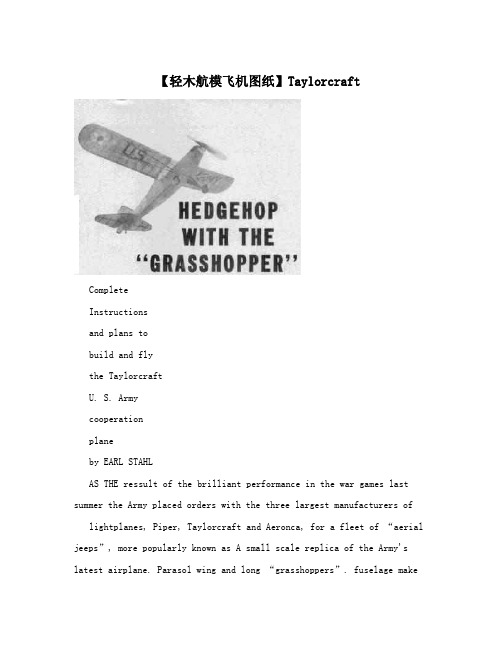
【轻木航模飞机图纸】TaylorcraftCompleteInstructionsand plans tobuild and flythe TaylorcraftU. S. Armycooperationplaneby EARL STAHLAS THE ressult of the brilliant performance in the war games last summer the Army placed orders with the three largest manufacturers of lightplanes, Piper, Taylorcraft and Aeronca, for a fleet of “aerial jeeps”, more popularly known as A small scale replica of the Army's latest airplane. Parasol wing and long “grasshoppers”. fuselage makeit an excellent contest model. The structure is simple, light Operating under simulated war conditions, and strong the "grasshopper fleet" proved that lightplanes are indispensable in modern warfare. Flown by civilian pilots, these planes proved their adaptability for all kinds of observation work, personnel carrying, directing traffic and troop movements, even picking-up and delivering massages, maps, and materials in flight.To further prove their value the "grasshoppers" repeatedly flew from seemingly impossible areas. In Louisiana army engineers prepared landing spots measuring a mere 400 ft. long and 100 ft. wide-and without considering wind direction. Obviously larger, faster planes could not use such bases, but these lightplanes in hands of skilled pilots made numerous takeoffs and landings. It was all in a day's work for pilots to land on highways, sometimes in open spaces between moving convoys, to complete a mission or possibly borrow a few gallons of gas. During maneuvers in Texas one pilot made several landings on the up-slope of a high mountain, then taxied around the gravel ledge rim, and took off on the down - slope. Of course there were a few accidents, but they were of a minor nature and quickly repaired. The most serious mishap resulted from a spin as a pilot cicled l ow so he could “Yoo-Hoo” to his girl friend."Grasshoppers" used in the war games were identical with ships available to civilians, all being converted tandem trainers powered by Continental 65 hp. engines. The only important additions were radio transmitters and receiver.For our model we have selected crosspiece centers under the upper formers shaft, then carve a right - hand propeller, the Taylorcraft trainer, known in the on the nose so they will not interfere with by cutting away the back, face of the Army as the O-57. This plane is similar in the rubber motor. Use the widest sheet blades until there is about 1/16" appearance, construction and performance available; cement it to the entire adjacent undercamber in each. Make each surface to other tandem trainers on the market. frame using pins and rubber bands to hold smooth and uniform with sandpaper. Available with Continental, Lycoming or it in place until dry. Extreme front of the Blade thickness is then easily determined Franklin engines of 65 hp., the nose is asolid block or laminations, as as the front is shaved away. Thin the commercial version performs as follows: shown. Roughly cut to shape, cut out hole blades as much as possible, still retaining Top speed, 102m.p.h.; landing speed, 35 for the nose plug, then cement to the desired strength. Round the tips like the m.p.h.; climb 600 ft. per min.; cruising fuselage front. When dry, cut the block to prop shown in the photos. Carefully sand range, 300 miles on 14 gallons of fuel. a smooth shape, then sand entire nose to and balance the prop as the final The model has the same fine shape. operation. Several coats of light dope, if characteristics as the real ship: Bend the two landing gear struts lightly sanded between each, will produce construction is easy and flight to shape and size shown from .040 music a smooth surface. A free - wheel gadget to performance is matched only by wire, attach to fuselage by neatly binding improve glide should be attached to the attractiveness. with thread and then applying several front and a bearing to the back.coats of cement. Join bottoms of the struts The nose plug is made fromby soldering or with thread and cement. laminated squares of 1/8" sheet with a CONSTRUCTION. -BeforeThe 1/16" sheet fill-in can be cut and 1/32" plywood front. Test flights of the starting, the fuselage plans should befitted but should not be attached until the original model showed that several joined: incidentally, if you do not want tofuselage is covered; the center struts degrees of both right and down thrust are mar your magazine, make tracings of thelikewise. desirable, so drill the hole in this manner. plans onsemi-transparent paper.Make full size plans of the right Cement washers to the front and back to First make the fuselageand left wing halves so parts call be fix the thrust line. underframe, of 3/32" sq. balsa longeronsassembled directly over them. Using the and cross-pieces, indicated by lightpatterns given, cut 18 of the regular and 2 shading. Make two side frames, one atop COVERING ANDof the tip ribs from soft 1/16" or 1/20" the other for identity; the cement will ASSEMBLY - Before the frames aresheet. Pin all like ribs together and sand to probably cause them to stick together but covered, they must be lightly butuniformity, then cut the notches with they can be separated by a razor blade. thoroughly sanded to remove all flaws andaccuracy. Pieces for the tips are cut from When dry, invert the side frames over a roughness. Colored tissue is used, banana1/8" sheet and assembled over the plan. complete top view plan and join with oil or light dope is the adhesive. CementTaper the 1/8" x 3/8" trailing edges before 3/32" sq. cross-pieces at the cabin. Next cellophane to side windows beforepinning to place over the plan. Pins keep pull the backs togetherand add remaining covering the fuselage. While performing the ribs in position. Spars are hard balsa; cross-pieces in the rear. Crack longerons the latter use numerous small pieces,the uppers being 1/16" sq. while the lower just in front of thecabin to pull sides carefully lapped, to avoid wrinkles; also are 3/32" sq. Leading edge is 1/8" x 1/4". together as shown. Check continually for cover the sheet balsa nose with tissue.Tilt the inner ribs a bit for correct correct alignment. Each sideof each wing half, stabilizer anddihedral. Cement all joints firmly, remove The various fuselage formers are rudder requires a separate piece of tissue,from plans and finish the leading edges shown; cut from each medium grade 1/16" tips, etc., require individual pieces, too.and tips by trimming with a razor and sheet. Cut the notches shown and cement Lightly spray all covered parts with watersandpapering. to place. Stringers are medium hard 1/16" to tightenthe covering - do not, howeverTail surfaces come next; both sq. strips: fit in the notches and cement apply any clear dope until later.stabilizer and rudder are of similar fast. From the cabin back stringers are Prepare to assemble parts byconstruction. Make complete frames using cemented directly to the sides of the under completing the fuselage. Cut a windshield1/16" sheet outlines, 1/16" x 1/8" strips for frame. Center section ribs, cut from 1/16" pattern from writing paper by the trial and spars and 1/16" sq. pieces for ribs. When sheet, are shown: two are needed with a error method; note the windshield extends dry, remove frames from the jigs and add third center cut as shown by the broken over the center section to the first1/16" sq. strips to every side of each rib. lines. Cement them to top longerons, crossmember. Once the pattern fitsThe ribs are later cut and sanded to against the inner edge leaving a 1/32" perfectly cut from celluloid and attachstreamline shape indicated. Taper leading ledge on which to later rest the wing with cement. The landing gear fill-in was and trailing edges to match the ribs. panels. Finish around the cabin by adding made previously and is cemented to theTo obtain fine flights from any the wedge-shaped pieces. The curved back wires. Cover the whole landing gear withflying scale model the propeller must be windows are cut from 1/16" sheet. tissue. The center landing struts areefficient. Select a hard block of proper Cover the nose with soft1/32" rounded bamboo splints with streamlinedimensions and cut the blank to shape sheet, but before installing remove the balsa covers at the top, representing shockshown. Drill the tiny hole for the propabsorber covers. Cement the bamboo to outlines, etc., etc., are all made with along the wing chord. Add weight to the the bottom of the struts but not the top so colored tissue. Tail wheel and similar nose if necessary to obtain this balance, they can spring apart. Wheels can be made parts are made from balsa scraps. since only minor, adjustments are made by from laminated discs of balsa or may be Additional details can be found on photos warping tail surfaces. Glide the model purchased. Cement bearings to the sides of of the big "grasshoppers" for those over deep grass making any further the wheels so they will revolve smoothly interested in reproducing every item. adjustments for a good glide. then place on the axles and hold in place Naturally any uncolored wood parts Power flight adjustments are with a drop of solder. should be doped to match the color made by off-setting the thrust line. Start Care must be exercised when scheme. with just a few turns - then use more assembling the surfaces to the fuselage to Bend the propeller shaft power as justified. Placing a sliver of wood keep everything in perfect alignment. First from .040 music wire. Slip the nose plug, between the tip of the nose plug and the cemet stabilizer to place; it is parallel to several washers and prop on the shaft in nose tilts the thrust line down, helping to the work bench. A tissue fillet is placed that order, then bend the shaft end as iron out stalls under power. Right or left from fuselage to stabilizer before the required for the free-wheeler. thrust helps to control the circles. rudder is set in position. Off-set the rudder Once the "bugs" that usually about 1/16" for a right circleglide. Wing show up in first tests are eliminated, use a FLYING - Depending on thetips must be dihedraled about 1-1/2" for mechanical winder to get maximum turns finished weight of the model, ten or twelve proper stability. Be sure to attach the and power from the rubber motor. Take strands of 1/8" brown rubber is requiredwings firmly. Wing struts are shown; care where you launch your for power. Lubricate the strands, hookassemble and color before cementing to "grasshopper," for the top of a tree or the them on the prop shaft and then drop theposition. The entire model is now given side of a building is hardly a suitable other end through the fuselage. As shown,one or two coats of clear dope. landing field; you have quite an a bamboo pin holds the motor in the rear.There are numerous minor details investment of time and effort in your If necessary, remove a small section ofadded to improve appearance. For the Taylorcraft - protect it with good covering to aid in getting the motor inmore ambitious builder the four - cylinder judgment. position.engine offers plenty of possibilities for The Taylorcraft "grasshopper" VICTORYdetail. Insignia, letters, control surface should balance at a point about 1/2 backA large high pitch prop gives it. long duration Scanned from April 1942Model Airplane NewsbyGarry T. Hunter。
音箱可靠性测试规范

HARMAN INTERNATIONALRELIABILITY TEST PLANforAUTOMOTIVE AUDIO SPEAKERharman consumer groupCentral Quality GroupRelease Date: 2/1/98 Revision Level: KRevision Level Date: 03/31/051.0 PurposeThe purpose of this test plan is to describe the environmental and functional performancerequirements to which the speaker will undergo in order to be validated. The intent of thevalidation program is to expose the speaker to an accelerated aging process.2.0 Test PlanThis test plan details the type of tests and the number of units required for each. The sample size outlined below may change depending on Reliability Target.2.1 Test ImplementationThe full qualification test program consists of the groups listed below. This is a parallel test sequence such that each group is run independently. This test plan must be performed on at least one member of a “Product Family”. The most complex or highest power model should be chosen.Full Qualification Test SequenceGroupQuantityDV PVTest Name Spec. Sect.No.Functional TestRequirementsA 2 6Life Cycle 5.1 4.4 and 4.5B 2 6Power Test 5.4 4.4 and 4.5UV Exposure Test 5.8Impact Test 5.5C 2 6Humidity Test 5.3 4.4 and 4.5Random Vibration Test 5.6 4.4 and 4.5D 2* 6 Packaging Test (ASTM) 5.7 4.4 and 4.5For Packages up to 150 lbs (ASTM4169)Handling (Drop), First Sequence 5.7.1 4.4 and 4.5Compression Test (Vehicle StackingAssurance Level II)5.7.2 4.4 and 4.5Loose Load Vibration 5.7.3 4.4 and 4.5Vehicle Vibration 5.7.4 4.4 and 4.5Handling (Drop), Second Sequence 5.7.5 4.4 and 4.5Temperature Test 5.2 4.4 and 4.5(1) For Master Pack Shipping Option (ifavailable)5.7.9Humidity Storage Test 5.7.9.1Loose Load Vibration 5.7.3VehicleVibration 5.7.4* If packaging is available.Note 1: Unless otherwise specified, all units shall be tested in the orientation that unit will be mounted in the car.Note 2: The performance limits of the units under test will be specified in the HCG approved Engineering Test Specification (ETS) [see Section 6].2.2 Abbreviated QualificationThe abbreviated test program consists of the groups listed below. This is a parallel test sequence such that each group is run independently. These tests must be performed on all members of a “Product Family” not subjected to the Full Qualification found in section 2.1.Abbreviated Qualification Test ScheduleGroupDV PV Test Name Spec. Sect.No.Functional TestRequirementsA 2 6Life Cycle 5.1 4.4 and 4.5B 2 6Power Test 5.4 4.4 and 4.5Handling Drop Test 5.5C 2* 6Packaging Test (ASTM) 5.7 4.4 and 4.5For Packages up to 150 lbs (ASTM4169)Handling (Drop), First Sequence 5.7.1 4.4 and 4.5Compression Test (Vehicle StackingAssurance Level II)5.7.2 4.4 and 4.5Loose Load Vibration 5.7.3 4.4 and 4.5Vehicle Vibration 5.7.4 4.4 and 4.5Handling (Drop), Second Sequence 5.7.5 4.4 and 4.5* If packaging is available.Note 1: Unless otherwise specified, all units shall be tested in the normal car mounting orientation.Note 2: The performance limits of the UUT will be specified in the Engineering Test Specification.3.0 Standard Test Conditions3.0.1 Signal SourceUnless otherwise specified, all tests shall be conducted with the Audio SignalGenerator/Amplifier output configured to be balanced, less than or equal to 50-ohm source impedance, and floating. The signal source GND shall be connected to the speaker PWRGND at the speaker.3.0.2 PositionUnless otherwise specified, the speaker shall meet all requirements in the “normal mounting position”. It is defined on the Product Specification as to the horizontal or vertical position of the mounting surface.3.0.3 Room TemperatureUnless otherwise specified, all measurements shall be made at room temperature. Roomtemperature is specified as 23o C +/-3o C.3.0.4 Frequency RangeThe frequency range is specified from the -3dB point at the upper and lower operating range of the driver. This range and the limits with in that range shall specified on the ProductSpecification.3.0.5 NoiseThe products are divided into three groups, full range (multi-element), mid-bass, and sub-woofer. The type of product shall be specified on the Product Specification.Full Range will use track 13 on the Car Audio Test Disc Version 2.0: IEC noise with acrest factor of 9dB.Mid-bass will use track 14 on the Car Audio Test Disc Version 2.0: a decade of pinknoise, 50 to 500Hz (-3dB points) 12dB slopes, with a crest factor of 9dB.Sub-woofer will use track 15 on the Car Audio Test Disc Version 2.0: a decade of pinknoise, 30 to 300Hz (-3dB points), 12dB slopes, with a crest factor of 9dB.3.0.6 Music SignalThe products are divided into two groups: 1) full range (multi-element) and mid-bass, 2) sub-woofer. The type of product shall be specified on the Product Specification.Full Range and Mid-bass – track 16 on the Car Audio Test Disc Version 2.0: “Beat It”by Michael JacksonSub-woofer – track 17 on the Car Audio Test Disc Version 2.0: “Crime Stories” by MCHammer4.0 Functional RequirementsFunctional requirements are to be tested in accordance with an HCG approved product engineering specification (ETS).4.0.1 PolarizationWith the driver face down and the terminal facing toward you the Product Specification shall identify the positive terminal, which shall be labeled Pin 1 or “+”. When a positive potential is applied to the positive terminal, the cone shall move outward from the basket producingpositive pressure.Ref. IEC 268-24.0.2 DC ResistanceEnsure that the test lead resistance is factored out of this measurement. Connect the test leads to the speaker and measure the resistance in ohms with an averaging ohmmeter to ensure that ambient noise levels do not produce an EMF at the meter yielding false resistance readings.The DCR shall be within the limits specified on the Product Specification.4.0.3 ImpedanceRigidly suspend the speaker from the motor structure in free air at least 50 cm from thenearest reflecting surface. Mounting means must be minimal in bulk such that the airmovement during testing is substantially unrestricted.Measure the deviation from the Reference Sample Speaker impedance at each of the definedfrequencies. The deviation at all frequencies shall be within the limits specified on the Product Specification.4.0.4 Frequency ResponseApply a stepped sine wave sweep or a Canetics signal over the specified frequency range,using the specified frequency spacing, with the specified bandwidth smoothing per theProduct Specification, and analyze the microphone output. Calibrate the measurement system to display the 1 Watt 1 Meter equivalent sensitivity based on Z nom as specified on the Product Specification. Display the SPL and the Frequency in ISO standard 25dB/decade aspect ratio.The resultant graph of amplitude vs. frequency is defined as the frequency response. Measure the deviation from the Reference Sample Speaker sound pressure level at each of the definedfrequency bands. The deviation at all frequencies shall be within the limits specified on theProduct Specification.To verify that no damage has occurred to the Reference Sample Speaker and that the testequipment is functioning properly, the first process shall be to test the Reference SampleSpeaker against the stored data from the previous production runs. If there is a change of more than one standard deviation at any frequency, both the Reference Sample Speaker and testequipment shall be re-calibrated.4.0.5 Extraneous NoiseThe speaker assembly shall not produce extraneous noise when a dynamic test is performed.The following types of deficiencies are some typical causes of extraneous noise:Buzz: Any noise produced by a looseness of components vibrating against othercomponents.Rub: Any noise produced by the voice coil sliding or rubbing against other components.Bottoming: The noise produced by the contact of the moving system with the speakerstructure.Rattle: The random noise produced by an object trapped within the speaker strikingmoving components or any intermittent noise caused by loose electrical connections orcontrols.Frozen Coil: Absence of free excursion caused by adhesive in the magnetic gap or anoffset (loose) component of magnetic circuit.Air Noise: The noise produced by high velocity airflow through a small leak.5.0 Qualification TestingThe reliability target for all car speaker products is zero defects at 50,000 miles operation.Successful completion of the test is intended to demonstrate 90% reliability with 90% confidence.5.1 Life CycleEach speaker shall withstand 5 cycles (totaling 215 hours) of the environmental conditionsoutlined below. The speakers should be checked once a day on a regular basis. A full functional test should be performed on all units at the end of the second and fifth cycles.5.1.1 Life Cycle CalibrationThe supplied Car Audio Test Disc Version 2.0 facilitates accurate test level calibration and testing consistency by incorporating sine wave test tones (first three tracks) that are calibrated to the music tracks specified for testing.Using the RMS number from the Product Specification under the “Life Cycle” column, the level will be calibrated with the appropriate test tone (track 1 for subwoofers, track 2 for mid-bass, and track 3 for multi-element full range). Then skip to track 16 “Beat It” for full range and mid-bass or track 17 “Crime Stories” for subwoofer and repeat for the specified duration.The level of the music signal is already calibrated to the test tone.A. Over a 30-minute period, raise the temperature to 40°C with a relative humidity of 95%.B. Stabilize the temperature at 40°C with a relative humidity of 95% for 16 hours. After 6 ½hours, apply the designated music signal at 1/8th the specified RMS voltage (section3.0.6). At the end of the 16-hour period, remove the signal.C. Over a 30-minute period, raise the temperature to 90°C with a relative humidity of <20%.D. Stabilize the temperature at 90°C with a relative humidity of 20% for 8 hours. After 3hours, apply the designated music signal at 1/8th the specified RMS voltage. At the end of the 8-hour period, remove the signal.E. Over a 30-minute period, lower the temperature to 25°C.F. Stabilize the temperature at 25°C for 2 hours.G. Over a 30-minute period, lower the temperature to -35°C.H. Stabilize the temperature at -35°C for 5 hours. After 2 hours, apply the designated musicsignal at 1/8th the specified RMS voltage. At the end of the 5-hour period, remove the signal.I. Over a 1-hour period, raise the temperature to 90°C.J. Stabilize the temperature at 90°C for 5 hours. After 2 hours, apply the designated music signal at 1/8th the specified RMS voltage. At the end of the 5-hour period, remove the signal.K. Over a 30-minute period, lower the temperature to 25°C.L. Stabilize the temperature at 25°C for 3.5 hours.M. This is the end of one cycle.(See graph on next page)5.2 Temperature (Non-Operational) TestEach speaker shall withstand 24 hours of exposure to -35o C and 24 hours to 90o C inside theenvironmental chamber. The test duration should be 24 hours at each temperature with aminimum of 4 hours between temperature conditions. Let the speakers cool down to a normal room temperature before any post-test evaluation is performed. The speaker should be tested at the end of each 24-hour period.Ref. Chrysler PF 9506 2.2.2.5 Temperature Test5.3 Humidity (Non-Operational) TestEach speaker shall withstand exposure to 40o C at 95% relative humidity for 16 hours, then 90o C at 20% relative humidity for 8 hours with 15 minutes ramp between the two temperature and humidity conditions. This is considered one cycle. The total test is 5 cycles long totaling 122 hours. Leave the speakers for a minimum of 4 hours at room temperature before any post-test evaluation is performed.Ref. Chrysler PF 9506 2.2.2.1 Damp/Dry Cycling5.4 Operating Power (Noise) TestEach speaker shall withstand 100 hours of application of noise signal specified in section 3.0.5.The noise signal should be calibrated to 100% of the RMS voltage rating as specified on the Product Specification. Leave the speakers for a minimum of 4 hours at room temperature before any post-test evaluation is performed.5.4.1 Power Test Calibration ProcedureThe supplied Car Audio Test Disc Version 2.0facilitates accurate test level calibration andtesting consistency by incorporating sine wave test tones (first three tracks) that are calibrated to the noise tracks specified for testing.Using the RMS number from the Product Specification under the “Power Test” column, the level will be calibrated as follows:Subwoofer – use track 1: 50 Hz 0 dBMid-bass – use track 2: 100 Hz 0 dBFull range (multi-element) – use track 3: 1 kHz 0 dBThen skip to the appropriate noise track (Subwoofer – track 15, Mid-bass – track 14, Fullrange – track 13) and repeat for the designated 100-hour duration of speaker testing. Thelevel of the test signal is already calibrated to the test tone.NOTE: The amplifier used in the test set-up must be capable of slightly higher PEAKvoltage than the level required for testing. An oscilloscope will be used to verify theabsence of a clipped output signal (which could cause damage to the transducer andpremature failure).5.5 Impact (Non-operational) TestEach speaker (without the packaging) shall withstand one (1) drop from a height of 1 meter onto a concrete base. Each speaker shall be dropped once for each side. A total of 6 units are needed to cover all six (6) sides.Each speaker shall be visually inspected for any loose or broken parts and components. Results of the test should be treated for information purposes only and not part of the acceptancecriteria.5.6 Random Vibration (Non-operational) TestEach unit shall withstand 2 hours per axis of the Random Vibration outlined below: Z – AxisBreakpoint (Hz) Magnitude (G2/Hz)0.005550.059100.035602000.00070.000041000Total Spectral Content = 1.8 GrmsY-AxisBreakpoint (Hz) Magnitude (G2/Hz)0.009250.07680.076120.00031000Total Spectral Content = 1.685 GrmsX-AxisBreakpoint (Hz) Magnitude (G2/Hz)0.00545100.05120.00271900.000233700.000231000Total Spectral Content = 1.4 GrmsPost TestTest units shall be visually inspected for any loose or broken parts and components, followed by functional testing.Ref. Chrysler PF 9825 2.3.2.1 Vibration5.7 Packaging Test (ASTM)5.7.1 Schedule A–Manual Handling, First SequenceFor purposes of this procedure, the bottom of a small parcel is the surface on which the parcel rests in its most stable orientation. Recommended drop heights, the number of drops, thesequence of drops, and the shipping unit orientation at impact are as follows:Shipping Weight, lb (kg) Drop Height, in. (mm)0 to 20 (0 to 9.1) 24 (610)20 to 40 (9.1 to 18.1) 21 (533)40 to 60 (18.1 to 27.2) 18 (457)60 to 80 (27.2 to 36.3) 15 (381)80 to 100 (36.3 to 45.4) 12 (305)100 to 200 (45.4 to 90.7) 10 (254)Number ofImpacts AtSpecified Height Impact Orientation –First Sequence of Distribution CycletopOneTwo adjacent bottom edgesTwo diagonally opposite bottom cornersbottomOneRef: ASTM D 4169 – 99Post TestThe units should be checked for functional performance and external appearance after the test.No impaired function or concealed damage is permitted. End pads may be cracked with no separation. Cartons should have no tearing or de-bonding of the seam edge.5.7.2Compression Test: Vehicle Stacking Assurance Level IISchedule B – Warehouse Stacking and Vehicle StackingThis test is intended to determine the ability of the shipping unit to withstand thecompressive loads that occur during warehouse storage or vehicle transport. Theformula calculates the compressive load over the largest footprint of the package usinga shipping density factor. A safety factor is used to take into effect time in storage,stacking pattern, variables in container strength and atmospheric conditions(temperature, humidity). The test is to be conducted by loading the shipping unit to thecomputed load value, as calculated below. The compressive load is to be uniformlydistributed about its largest footprint. Remove the load within 3 seconds after reachingthe specified value.Formula:L = Mf*J*((l*w*h)/K)*((H-h)/h)*FL = Minimum Required Test Load=lb or NMf = Shipping Cargo Density factor = 10.0 lb/ft3 or 160 kg/m3J = conversion factor = 1 lbf/lb or 9.8 N/kgl = length of shipping unit = in or mw = width of shipping unit = in or mh = height of shipping unit = in or mK = conversion factor = 1728 in3/ft3 or 1 m3/m3H = maximum stack height = 108.0 in or 2.7mF = factor to account for individual factors described above = 7Acceptance Criteria:1. No visible damage2. Product intact internally3. Packaging components able to provide further protection4. Compression test cannot cause the outer shipping container to crease, split or tear at the joint.Test Conditioning: 73.4o F (+/-2o F) [23o C (+/-1o C)] and 50% (+/-2%) relative humidity in accordance with practice D 4332.Ref: ASTM D 41695.7.3 Loose Load Vibration Method A1—Repetitive Shock TestPlace the test specimen on the test machine platform in its normal shipping orientation. Attach restraining devices to the platform to prevent the specimen from moving horizontally off the platform and to prevent excessive rocking without restricting the vertical movement. Adjust the restraining devices to permit free movement of the specimen of approximately 10 mm (0.4 in.) in any horizontal direction from its center position. Start the vibration of the platform at a frequency of about 2 Hz and steadily increase the frequency until some portion of the test specimen repeatedly leaves the test surface. To ensure that the test specimen receives acontinuing series of repetitive shocks, a shim with a 1.6 mm (1 /16 -in.) thickness and a width of 50 mm (2.0 in.) shall be used to determine when the test specimen is leaving the testplatform. The shim should be inserted under the package a minimum of 100 mm (4.0 in.) and moved intermittently along one entire length of the package.Continue the test at this frequency for a period of 1 hour. The test may be stoppedmomentarily to inspect for damage.If the container might possibly be transported in any other orientations, test at least onecontainer in each possible orientation for the full-specified test duration.Inspect the container and its contents and record any damage or deterioration resulting from the test.Ref: ASTM D 4169 – 99, ASTM D 999 – 965.7.4 Schedule E-Vehicle VibrationPerform the test for each possible shipping orientation. Recommended intensities anddurations for the random tests are given below.Random Test:The following power spectral densities (as defined by their mode of transport, frequency and amplitude breakpoints) and test durations are recommended:Air: Assurance Level IFrequency, Hz Power Spectral Density Level, g 2 /Hz0.000420.02120.021000.00002300Overall, g rms 1.49Duration, min B180B For vehicle vibration tests in multiple shipping unit orientations, the total duration should bedistributed evenly between the orientations tested.Ref: ASTM D 4169 - 995.7.5 Schedule A–Manual Handling, Second SequenceFor purposes of this procedure, the bottom of a small parcel is the surface on which the parcel rests in its most stable orientation. Recommended drop heights, the number of drops, the sequence of drops, and the shipping unit orientation at impact are as follows:Shipping Weight, lb. (kg) Drop Height, in. (mm)0 to 20 (0 to 9.1) 24 (610)20 to 40 (9.1 to 18.1) 21 (533)40 to 60 (18.1 to 27.2) 18 (457)60 to 80 (27.2 to 36.3) 15 (381)80 to 100 (36.3 to 45.4) 12 (305)100 to 200 (45.4 to 90.7) 10 (254)Number ofImpacts AtSpecified Height Impact Orientation –Second Sequence of Distribution CycleOne vertical edgeTwo adjacent side facesTwo one top corner and one adjacent top edgeOne the drop should be in the impact orientation most likely for adrop to occur, usually the largest face or the bottom. Fordistribution cycles where any drop orientation is possible (i.e.,small parcel environment), this drop should be in the mostcritical or damage–prone orientation.Ref: ASTM D 4169 – 99Post TestThe units should be checked for functional performance and external appearance after the test.No impaired function or concealed damage is permitted. End pads may be cracked with no separation. Cartons should have no tearing or de-bonding of the seam edge.5.7.9 Master Pack Shipping Option (if available)This test is intended to determine the ability of the individual beauty boxes in a mastershipping carton to withstand the potentially abrasive environment that could occur during vehicle transport following warehouse storage. A master pack is considered to be at least six units in a larger carton. If the product master pack is less than this number, then additional master packs will be tested until the six individual unit requirement is met.The test samples will be repacked in previously untested beauty boxes free of any visibledefects before being packed in the master pack for this test. Samples will complete theHumidity Storage test in the master carton.5.7.9.1 Humidity Storage TestThe units shall be exposed to the following conditions:ConditionTemperature 40° C (+/-2° C)-2%/+3%Humidity 93%Exposure Time 48 hoursStabilization Time AfterMinimum of 8 hoursTest*Unit Configuration With Packaging*Stabilization Time is referred to as the elapsed time the unit has been out of theenvironmental chamber and allowed to reach ambient temperature and humidityconditions before continuing into the next test.The master pack will complete the Loose Load Vibration test (5.7.3). This will be followed by the Vehicle Vibration test (5.7.4).Post TestAfter the test the individual unit beauty boxes must be checked for appearance. No visiblesurface abrasion or carton degradation is permitted.5.8 Ultraviolet (UV) Exposure TestEach speaker should be place inside the UV test chamber and withstand 20 cycles of UVexposure test outlined below. The type of UV lamp should be 40 watts UV-C lamp as shown: Test Set Up:Environmental conditions as follows:Temperature is 90° C constant.Over a 30-minute period, raise the humidity from ambient to 90%.Maintain at this level for 2 hours.At the end of 2 hours, discontinue the humidity (allow to return to ambient).Continue at 90° C constant for 5 hours 30 minutes.This is one cycle (eight hours). Total test duration is 20 cycles.UV Test Environmental Profile:Int 1Post TestTest units shall be visually inspected for any degradation in parts and components, followed by functional testing. Cone and surround material should not become brittle or crack and there should be no de-bonding cone-to-dust cap or cone-to-surround. Some discoloration or fading is expected.6.0 PRODUCT SPECIFICATIONTEST PARAMETER SECTIONPosition 3.2 Hor/VertFrequency Range 3.4 Range +dB -dBNoise 3.5 Product Type RMSLevelPolarization 4.1 Lt/RtDC Resistance 4.2 Min Max NomOhmsMaxMinImpedance 4.3RangeOhmsOhms Frequency Response 4.4 Range +dB -dB。
A Meandered Loop Antenna for LTE/WWAN Operations in A Smart Phone
Progress In Electromagnetics Research C,Vol.16,147–160,2010A MEANDERED LOOP ANTENNA FOR LTE/WW AN OPERATIONS IN A SMART PHONEC.-W.Chiu and C.-H.ChangDepartment of Electronic EngineeringNational Ilan UniversityIlan260,TaiwanY.-J.ChiDepartment of Electrical EngineeringNational Chiao-Tung UniversityHsinchu350,TaiwanAbstract—This paper presents a multiband meandered loop antenna for smart phone applications.The proposed antenna which features a meandered folded-loop generates two resonance modes in the LTE/GSM bands.The current distributions of the excited resonance modes are analyzed to investigate the mode characteristic.By using a capacitively coupled feed on the backplane,the impedance bandwidth is broadened to cover LTE/WWAN bands.The simulation performed in this research used a high frequency structure simulator (HFSS)to optimally design the antenna,and a practical structure was constructed for the test.Details of the various antenna parameters are presented and discussed in this paper.1.INTRODUCTIONLTE(Long Term Evolution)is a new high-performance air interface standard for cellular mobile communication systems.It is the last step toward the4th generation(4G)of radio technologies designed to increase the capacity and speed of mobile telephone networks.LTE provides ultra-broadband speeds for mega multimedia applications by using a high performance antenna[1].The frequency spectrum allocated for LTE applications ranges from600MHz to3GHz,and Received25July2010,Accepted13September2010,Scheduled26September2010 Corresponding author:C.-W.Chiu(alexchiu@).148Chiu,Chang,and Chi the LTE band12–14covers from698MHz to798MHz.For the incorporation of the LTE band with the existing cellular phone,the operating bandwidth of a handset should cover from698MHz to 960MHz and from1710to2690MHz[1].In order to include LTE700/LTE2300/LTE2500,Wong and Chen recently proposed a small-size printed loop antenna integrated with two stacked coupled-fed shorted strip monopoles for multiband operation in a mobile phone[2].Some published papers proposed a multi-input and multi-output(MIMO)antenna configuration for LTE handset application in order to deliver ultra-broadband speeds for mega multimedia applications[3,4].Since the spectrum for the LTE700 system is allocated at700MHz bands,the operating wavelength is longer than400mm.The ground plane size of a typical handset(say 100mm)is only about a quarter-wavelength.As a result,the chassis of a traditional monopole or PIFA in the handsets is a resonator.The resonating currents are spread out over the system’s ground plane[5–8].To avoid degrading of the antenna performance,a loop antenna is a good candidate for a LTE system.The performance of the loop antenna is less dependent on the ground plane,thus it is suitable for a LTE antenna design[9].The main current distribution of the loop antenna is limited in the closed loop pattern and feed port.Therefore, handheld and head proximity influences are reduced since the current of the loop antenna on the ground plane is less than that of the PIFA or monopole[10–14].In this paper,a compact internal antenna which operates in the LTE/GSM and PCS/UMTS/WLAN/LTE2300bands is proposed.The antenna is a kind of folded loop which is fed by a back-coupling element connected to a microstrip transmission line[15].A parallel monopole-like mode and a combination mode formed by loop pattern and device chassis are excited to cover the bandwidth from698MHz to960MHz. This design is easily to be implemented in a double-sided printed circuit board.The occupied geometrical space of the antenna structure measures only60mm×10mm×6.5mm.The proposed antenna design is described in Section2,and a parameter study on analyzing the effect of some critical parameters is also presented.Experimental results of the proposed prototype are presented and discussed in Section3.2.ANTENNA DESIGN AND ANALYSIS2.1.Antenna DesignFigure1(a)shows the three-dimensional configuration of the proposed antenna.The antenna is mounted on a0.8-mm thick FR4substrate with a relative permittivity of4.4and a loss tangent of0.02.TheProgress In Electromagnetics Research C,Vol.16,201014960110unit: mm6.550Ω microstrip feeding line on the back sideground plane 60x100CDFYZ XH27.527.5strip line A(a)(b)unit:mmn=22m =17.7d=650 Ω microstrip feeding line29.2529.25 Lg=1001ground plane on the back side 100 x 60top edge of ground plane (on the back side )coupling elementtuning stub(c)Figure 1.Geometry of the proposed antenna.(a)3D view,(b)plan view of the front-side,and (c)plan view of the back-side.antenna system consists of a folded loop strip and a capacitively-coupled feeding line.The loop pattern is meandered and folded to increase the electrical length but at the same time reduce the size it occupies.The total length of the folded and meandered loop strip from C to D is about 286mm,as shown in Fig.1(b).To excite a new resonant mode by coupling,a strip line A is arranged directly above the coupling element on the back plane.To increase electric length and support the meandered loop,a tuning strip line B is inserted into the loop.On the same side of the substrate,a copper plate which is 60mm wide and 100mm long is printed to act as the system ground plane of a smart phone.To broaden the impedance bandwidth,an inverted L-shape coupling element with a matching stub,as shown in Fig.1(c),is placed on the back side and connected to the feed port.The150Chiu,Chang,and Chicoupling feed scheme generates two resonance modes in the LTE/GSM band.The coupling element on the backplane is connected to a 50ohm microstrip line with a strip width of 1.5mm.Figure 2(a)shows the simulated reflection coefficient for the folded loop antenna fed by the capacitively-coupled microstrip line compared with the one fed directly by a coaxial cable at point C shown in Fig.1(b).Basically,a parallel monopole-like mode,which its current path is from point D,through E,G,to H,is excited on the loop pattern by the unbalance-fed scheme.If the antenna is fed directly,the monopole-like mode is generated on the two arms from D to H and C to H in the lower GSM band.The field of the antenna system with the direct feeding scheme is inductively coupled to the ground plane.Since the maximum magnetic field is located at the center of the ground plane,not near the rim of the conductor plane,the antenna system cannot generate a chassis wavemode.However,two resonating modes are excited when the antenna is capacitively fed on the backside of the substrate because the maximum electric field of the chassis mode is close to the rim of the ground plane.Hence,the PCB resonance mode is easily excited by capacitive coupling.As a result,the impedance bandwidth could be broadened to cover the LTE/GSM850/GSB900bands.Figure 2(b)shows the input impedance when the antenna is fed by the two different feed schemes.The reactance of the impedance in the low band is inductive when the antenna is fed directly by a cable at point C.This inductive reactance has a high rate of change with respect to frequency so as to limit the bandwidth;therefore,the PCB chassis mode cannot be generated.Consider the loop antenna has a back-coupled feed port.The inductive reactance is compensated by theFrequency (GHz)R e f l e c t i o n C o e f f i c i e n t (d B )direct feedingcapacitively-coupling-6dBR e [Z i n ](Ω)I m [Zi n](Ω)Frequency (GHz)0.511.522.53-30-25-20-15-10-50200400600800(a)(b)Figure 2.Simulated results of (a)the reflection coefficient and (b)the input impedance with different feed schemes.Progress In Electromagnetics Research C,Vol.16,2010151Frequency (GHz)R e f l e c t i o n C o e f f i c i e n t (d B )Figure 3.Simulated results of the reflection coefficient with strip lines A and B.capacitively coupled element to form a self-complimentary impedance so as to widen the impedance bandwidth (red line).The input signal launched from the inverted-L-shape feed line capacitively couples to strip line A.Strip line A helps to excite a new resonant mode.Fig.3shows the reflection coefficient for the antenna with and without strip lines A and B.A new loop mode is excited when strip line A is inserted.The new chassis-handset combination,which is generated from point C’,through F,E,G to H and C’,is supported by the coupled structure with strip line A,as Fig.1(b)shows.On the other hand,a parasitic line B is inserted into the loop to increase the electrical length of the lowest resonance frequency and support the folded loop.When inserting the strip lines A and B,this study finds that the bandwidth is broadened because two modes are generated in the low GSM band.2.2.Current DistributionThe surface current distribution on the conductor strip confirms the mode characteristic.Fig.4shows the vector current distributions at 720and 990MHz.The current behavior demonstrates that the monopole-like mode creates the resonance at 720MHz and the antenna-chassis combination mode at 990MHz,respectively.These results are simulated by a commercial electromagnetic simulation tool,HFSS.The strip ends of the loop antenna structure symmetrically terminate to the ground plane.The currents on both sides of the loop are of the same phase at 720MHz with respect to the central feed line,as Fig.4(a)shows.Thus,the antenna behaves like two parallel folded monopoles at 720MHz.The quarter wavelength at 720MHz is calculated to be around 104mm but the meander length of one arm,as shown in152Chiu,Chang,and Chi(a)(b)Figure4.Simulated vector current distributions and surface current densities.(a)720MHz,(b)990MHz.Progress In Electromagnetics Research C,Vol.16,2010153Fig.1(b),is around 141.5mm.The physical length of the wavelength of the monopole-like mode is longer than the electrical length due to fold and meander.The monopole-like mode can also be verified by the radiation patterns discussed in Section 3,where E Θin the x -y plane is basically omni-directional.The current behavior in Fig.4(b)shows that the antenna-chassis combination mode is excited at 990MHz.Since the proposed antenna has an unbalanced feeding scheme,the currents are generated on the groundplane,and therefore,the ground plane is operated as a part of a radiator.Since the ground length is smaller than half-wave length below 1GHz,the resonance mode at 990MHz uses the printed circuit board of the mobile terminal as part of the antenna.The characteristic wave modes of the PCB conductor have contribution on the combined radiation behavior of the PCB and the loop element.The radiation mode is characterized as the combination of the handset antenna and the PCB conductor [16].The current distribution at 990MHz shows that it doesn’t form complete resonance current path in the loop pattern.The antenna element dominantly acts as a coupling element at 990MHz.Therefore,the antenna system can be modeled as a dual-resonant circuit [16].The radiation mode due to the groundplane resonance enhances the bandwidth when the antenna system is properly designed [7].Fig.5shows the effect of ground length Lg on the antenna performance,and observations showed larger effects on the resonance modes in the low band.The longer the length,the greater the bandwidth [7,16].Frequency (GHz)R e f l e c t i o n C o e f f i c i e n t (d B )Figure 5.Simulated results as a function of length L g (system ground planelength).-5Frequency (GHz)R e f l e c t i o n C o e f f i c i e n t (d B )Figure 6.Simulated results as a function of length m .154Chiu,Chang,and ChiFrequency (GHz)R e f l e c t i o n C o e f f i c i e n t (d B )Figure 7.Simulated results as a function of length n of the tuning stub.Frequency (GHz)R e f l e c t i o n C o e f f i c i e n t (d B )Figure 8.Simulated results as a function of distance d of the tuning stub.2.3.Parametric AnalysisTo obtain better impedance matching,an inverted L-shape coupling element with a tuning stub is connected to the feeding microstrip line on the back plane.The design of the coupling element is a critical factor.This research conducted a parametric study on the length m and the stub length n shown in Fig.1(c).When the parameter m varies between 14.7to 24.7mm or the parameter n varies from 19to 25mm,the rest of the dimensions of the antenna remain the same as shown in Fig.1.Fig.6shows the simulation reflection coefficient as a function of length m .Length m plays an important role in exciting the second mode in the low band.The variation in length has a substantial influence on the impedance matching in the design bands.Fig.7shows the simulation reflection coefficient as a function of stub length n .The findings show that the stub length n has a larger effect in the higher band.When the length is tuned to about 22mm,the bandwidths in the low band and the higher band achieve the bandwidth requirement of −6dB.Fig.8shows the simulation reflection coefficient as a function of d which is the distance from the ground plane edge to the tuning stub shown in Fig.1(c).When distance d is fixed at 6mm,the impedances are well matched in the higher band.3.RESULTS OF THE PROPOSED ANTENNAThe proposed antenna was constructed for testing purposes.The measurements were performed using an Agilent E5071B network analyzer.Fig.9shows the measured and simulated reflectionProgress In Electromagnetics Research C,Vol.16,2010155Frequency (GHz)R e f l e c t i o n C o e f f i c i e n t (d B )Figure 9.Measured results compared with simulation results.coefficient of the proposed antenna.The simulated results were obtained using Ansoft HFSS.There was a good agreement between the measurement and simulation below 1.8GHz.The finding shows that the achieved bandwidth covers the LTE/GSM850/GSM900band and PCS/UMTS/WLAN/LTE2300.In the low band,the achieved bandwidth with reflection coefficient better than −6dB was 423MHz (675–1098MHz)and in the high band it was 870MHz (1760–2630MHz).Figure 10shows the measured and simulated radiation patterns of the proposed antenna on the XY plane.The radiation-pattern and gain measurements were performed in the anechoic chamber of SGS pany in Taiwan.The radiation patterns E Θare nearly omni-directional in the xy -plane.These features are desirable characteristics for mobile phones.Fig.11shows the measured peak gains and radiation efficiencies.The peak gains and the radiation efficiencies were measured using the ETS-Lindgren model AMS-8500antenna measurement system and the 3164-08open boundary quad-ridged horn antenna,respectively.The measured antenna gain over the low band varied from around 1.5–3.0dBi and the radiation efficiency was higher than 50%.The measured antenna gain for the higher band varied around 1–4.2dBi and the radiation efficiency was larger than 50%,ranging from 1.8to 2.5GHz.Since the connecting semi-rigid coaxial cable (about 30cm)between the DUT and the testing system of SGS is not wrapped by a choke or a ferrite bead,the connecting cable used in the measurement acts as a radiator in the lower band (below 1GHz)due to the currents traveling on its outer face [17].The additional radiation from the outer conductor of the cable has some impact on the gain.Therefore,the measured gain is larger than that156Chiu,Chang,and Chiof ordinary monopoles in the lower band.The specific absorption rate (SAR)of the proposed antenna was studied using the FEKO simulation software [18].Fig.12shows the simulation model with the antenna placed at the cheek position near the phantom.The phantom of the head model used in SAR computation is a specific anthropomorphic mannequin (SAM)defined by the IEEE Standards Coordinating Committee 34[19].The separation distance between the system ground plane and the earpiece of the SAR phantom head is 5mm.The tilted angle between the center2045MHz2350MHzX-Y planeY270180270180(d)(e)Figure 10.Measured and simulated radiation patterns at 745MHz,850MHz,925MHz,2.045GHz,and 2.35GHz,respectively.line of the printed circuit board and the vertical line of the phantom is 63◦.The antenna is placed at the top edge of the system ground plane or at the bottom position (rotating 180◦).The testing power is 24dBm (0.25W)for the GSM850/GSM900/UMTS bands,while the testing power is 20.8dBm (0.121W)for the DCS/PCS bands.Table 1lists the simulated 1-g average SARs at the transmitting frequencies of 836.6,914.8,1747,1880,and 1950MHz.The finding shows that the SAR at the bottom position is lower than that at the top position owing to the larger distance to the cheek.It seems that placing the antenna at the bottom edge is more promising for practical mobile phone applications.Table 1.Simulated 1-g average SAR(W/kg)at GSM850/GSM900-/DCS/PCS/UMTS bands.Band GSM850GSM900DCS PCS UMTS Frequency (MHz)f =836.6f =914.8f =1747f =1880f =1950At the top (W/kg) 1.866 1.887 1.734 1.712 3.281At the bottom(W/kg)1.1771.1490.7390.8911.458Frequency (GHz)A n t e n n a G a i n (dB i )R a d i a t i o n E f f i c i e n c y (%)A n t e n n a G a i n (dB i )R a d i a t i o n E f f i c i e n c y (%)Frequency (GHz)(a)(b)Figure 11.Measured peak gain and radiation efficiency,(a)in the low band and (b)in the higher band.Figure12.Simulation model with the proposed antenna for the SAR analysis.4.CONCLUSIONThis paper proposes a folded and meandered loop antenna for smart phone applications.By using a capacitively coupled feed on the back plane,two resonance modes excited on the meandered loop pattern and the ground plane have been demonstrated to achieve wideband in the lower band.The parametric study on the coupling element was performed to optimally design the folded loop antenna. The measured results on the constructed antenna were presented to validate the proposed design.The achieved bandwidth ranges from675to1098MHz and1760to2630MHz,and the measured results indicate that they cover LTE and WWAN bands.Since the proposed loop antenna is designed to include the new emerging LTE700/LTE2300/LTE2500bands,it is very suitable for the use in the4G smart phone.ACKNOWLEDGMENTWe are grateful to the National Center for High-performance Computing for the HFSS computer time and use of facilities.Also, the authors would like to thank Mr.Yu-Chou Chuang and Mr.Cheng-Chang Chen,Bureau of Standards,Metrology and Inspection, M.O.E.A,Taiwan,for their help in the SAR simulation using the FEKO simulation tool.REFERENCES1.Sesia,S.,I.Toufik,and M.Baker,LTE—The UMTS Long TermEvolution:From Theory to Practice,Wiley,Chichester,UK,2009.2.Wong,K.L.and W.Y.Chen,“Small-size printed loo-typeantenna integrated with two stacked coupled-fed shorted strip monopoles for eight-band LTE/GSM/UMTS operation in the mobile,”Microwave and Optical Technology Letters,Vol.52,No.7, 1471–1476,Jul.2010.3.Chaudhury,S.K.,H.J.Chaloupka,and A.Ziroff,“NovelMIMO antennas for mobile terminal,”Proceedings of the1st European Wireless Technology Conference,330–333,Amsterdam, Netherlands,Oct.2008.4.Bhatti,R.A.,S.Yi,and S.O.Park,“Compact antenna arraywith port decoupling for LTE-standardized mobile phones,”IEEE Antennas and Wireless Propagation Letters,Vol.8,1430–1433, 2009.5.Abedin,M.F.and M.Ali,“Modifying the ground plane and itseffect on planar inverted-F antennas(PIFAs)for mobile phone handsets,”IEEE Antennas and Wireless Propagation Letters, Vol.2,226–229,2003.6.Anguera,J.,I.Sanz,A.Sanz,A.Condes,D.Gala,C.Puente,and J.Soler,“Enhancing the performance of handset antennas by means of groundplane design,”IEEE International Workshop on Antenna Technology:Small Antennas and Novel Metamaterials (IWAT),29–32,New York,USA,Mar.2006.7.Cabedo, A.,J.Anguera, C.Picher,M.Rib´o,and C.Puente,“Multi-band handset antenna combining PIFA,slots,and ground plane modes,”IEEE Transactions on Antennas and Propagation, Vol.57,No.9,2526–2533,Sep.2009.8.Picher,C.,J.Anguera,A.Cabedo,C.Puente,and S.Kahng,“Multiband handset antenna using slots on the ground plane: Considerations to facilitate the integration of the feeding transmission line,”Progress In Electromagnetics Research C, Vol.7,95–109,2009.9.Lin,C.I.and K.L.Wong,“Internal meandered loop antenna forGSM/DCS/PCS multiband operation in a mobile phone with the user’s hand,”Microwave and Optical Technology Letters,Vol.49, No.4,759–765,Apr.2007.10.Chi,Y.W.and K.L.Wong,“Internal compact dual-band printedloop antenna for mobile phone application,”IEEE Transactions on Antennas and Propagation,Vol.55,No.5,1457–1462,May2007.11.Wong,K.L.and C.H.Huang,“Printed loop antenna witha perpendicular feed for penta-band mobile phone application,”IEEE Transactions on Antennas and Propagation,Vol.56,No.7, 2138–2141,Jul.2008.12.Chi,Y.W.and K.-L.Wong,“Compact multiband folded loopchip antenna for small-size mobile phone,”IEEE Transactions on Antennas and Propagation,Vol.56,No.12,3797–3803,Dec.2008.13.Chiu,C.W.,C.H.Chang,and Y.J.Chi,“Multiband foldedloop antenna for smart phones,”Progress In Electromagnetics Research,Vol.103,123–136,2010.14.Chiu,C.W.and Y.J.Chi,“Printed loop antenna with a U-shaped tuning element for hepta-band laptop applications,”IEEE Transactions on Antennas and Propagation,Vol.58,No.11, Nov.2010.15.Li,W.Y.and K.L.Wong,“Seven-band surface-mount loopantenna with a capacitively coupled feed for mobile phone application,”Microwave and Optical Technology Letters,Vol.51, No.1,81–88,Jan.2009.16.Vainikainen,P.,J.Ollikainen,O.Kivekas,and K.Kelander,“Resonator-based analysis of the combination of mobile handset antenna and chassis,”IEEE Transactions on Antennas and Propagation,Vol.50,No.10,1433–1444,Oct.2002.17.Chen,Z.N.,N.T.Yang,Y.X.Guo,and M.Y.W.Chia,“An investigation into measurement of handset antennas,”IEEE Trans.Instrumentation and Measurement,Vol.54,No.3,1100–1110,Mar.2005.18.FEKO,EM Software&Systems—S.A.(Pty)Ltd.(EMSS),[Online],available:.19.Beard, B. B.and W.Kainz,“Review and standardization ofcell phone exposure calculations using the SAM phantom and anatomically correct head models,”Biomed.Eng.Online,Vol.3, 34,Oct.13,2004.。
中国民用航空技术标准规定 独立式北斗机载导航有源双频天线(B1C 和B2a 频段)-英文版

Number:CTSO-2C608Date of approval:March 24,2023Approved by:Yang Zhenmei China Civil Aviation Technical Standard Order This China Civil Aviation Technical Standard Order (CTSO) is issued according to Part 37 of the China Civil Aviation Regulations (CCAR-37). Each CTSO is a criterion which the concerned aeronautical materials, parts or appliances used on civil aircraft must comply with when it is presented for airworthiness certification.Independent BDS Airborne Active Navigation Antennafor the B1C and B2a Frequency Bands1.Purpose.This China Civil Aviation Technical Standard Order (CTSO) is applicable to the manufacturers of the Project Approval for application of CTSO authorization (CTSOA) for independent BDS(BeiDou Navigation Satellite System) airborne active navigation antenna for the B1C and B2a frequency bands. This CTSO specifies the minimum performance standards(MPS) that independent BDS airborne active navigation antenna for the B1C and B2a frequency bands must first meet for approval and identification with the applicable CTSO marking.2.Applicability.This CTSO affects new application submitted after its effective date. Major design changes to article approved under this CTSO will require a new authorization in accordance with section 21.353 of CCAR-21R4.3. RequirementsThe equipment manufactured on or after the effective date of this CTSO and intended to be marked with this CTSO mark shall meet the minimum performance standards specified in Appendix 1 of this CTSO.a. Functionality.This CTSO standard is applicable to the independent BDS airborne active navigation antenna for the B1C and B2a frequency bands used to receive signals from the BDS and provides signals for the independent BDS airborne navigation equipment used in the en-route phases of the aircraft certified according to CCAR-23, CCAR-25, CCAR-27, CCAR-29 and CCAR-31.b. Failure Condition Classifications.(1) Failure of the function defined in Section 3.a is a minor failure condition if it causes erroneous information.(2) Loss of the function defined in Section 3.a is a failure condition without safety impact.(3) Design the system to at least these failure condition classifications.c. Functional Qualification.The test conditions specified in Appendix 1 of this CTSO shall prove that the performance of the equipment meets the requirements.d. Environmental Qualification.According to the test conditions in Appendix 1 of this CTSO, the standard environmental conditions and test procedures applicable to the equipment shall be adopted to prove that the performance of the equipment meets the requirements. In addition to RTCA/DO-160G, the applicant may also adopt other applicable standard environmental conditions and test procedures.Note 1:Some performance requirements in Appendix 1 are not required to be tested under all conditions contained in RTCA/DO-160G. If it can be shown that these specific performance parameters are not easily affected by environmental conditions according to calculation analysis, comparative analysis of similar designs, etc. and that the performance levels specified in Appendix 1 are not significantly reduced by exposure to such special environmental conditions, then this Class tests can be ignored.e.Software Qualification.If the article includes software, develop the software according to RTCA/DO-178C, Software Considerations in Airborne Systems and Equipment Certification, dated December 13, 2011, including referenced supplements as applicable, to at least the software level consistent with the failure condition classification defined in paragraph 3.b of this CTSO. The applicant may also develop the software according to RTCA/DO-178B, dated December 1, 1992.f.Electronic Hardware Qualification.If the article includes complex custom airborne electronic hardware, develop the component according to RTCA/DO-254, dated April 19, 2000, Design Assurance Guidance for Airborne Electronic Hardware, to at least the design assurance level consistent with the failure condition classification defined in paragraph 3.b of this CTSO. For custom airborne electronic hardware determined to be simple, RTCA/DO-254, paragraph1.6 applies.g. Deviations.For using alternative or equivalent means of compliance to the criteria in this CTSO, the applicant must show that the equipment maintains an equivalent level of safety. Apply for a deviation under the provision of 21.368(a) in CCAR-21R4.4. Marking.a. Mark at least one major component permanently and legibly with all the information in 21.423(b) of CCAR-21R4. The marking must include the serial number.b. Also, mark the following permanently and legibly, with at least the manufacturer’s name, subassembly part number, and the CTSO number:(1) Each component that is easily removable (without hand tools);(2) Each subassembly of the article that manufacturer determinedmay be interchangeable.c. If the article includes software and/or airborne electronic hardware, then the article part numbering scheme must identify the software and airborne electronic hardware configuration. The part numbering scheme can use separate, unique part numbers for software, hardware, and airborne electronic hardware.d. The applicant may use electronic part marking to identify software or airborne electronic hardware components by embedding the identification within the hardware component itself (using software) rather than marking it on the equipment nameplate. If electronic marking is used, it must be readily accessible without the use of special tools or equipment.5. Application Data Requirements.The applicant must furnish the responsible certification personnel with the related data to support design and production approval. The application data include a statement of conformance as specified in section 21.353(a)(1) in CCAR-21R4 and one copy each of the following technical data:a. A Manual(s) containing the following:(1) Operating instructions and equipment limitations sufficient to describe the equipment’s operational capability.(2) Describe in detail any deviations.(3) Installation procedures and limitations sufficient to ensure that the antenna equipment, when installed according to the installation or operational procedures, still meet this CTSO’s requirements. Limitations must identify any unique aspects of the installation. The limitations must include a note with the following statement:“This article meets the minimum performance and quality control standards required by a CTSO. Installation of this article requires separate approval.”(4) For each unique configuration of software and airborne electronic hardware, reference the following:(i) Software part number including revision and design assurance level;(ii) Airborne electronic hardware part number including revision and design assurance level;(iii) Functional description.(5) A summary of the test conditions used for environmental qualifications for each component of the article. For example, a form as described in RTCA/DO-160G, Environmental Conditions and Test Procedures for Airborne Equipment, Appendix A.(6) Schematic drawings, wiring diagrams, and any other documentation necessary for installation of the antenna equipment.(7) List of replaceable components, by part number, that makes upthe airborne equipment. Include vendor part number cross-references, when applicable.b. Instructions covering periodic maintenance, calibration, and repair, for the continued airworthiness of the antenna equipment. Include recommended inspection intervals and service life, as appropriate.c. If the article includes software: a plan for software aspects of certification (PSAC), software configuration index, and software accomplishment summary.d. If the article includes hardware: a plan for hardware aspects of certification (PHAC), hardware configuration index and hardware completion accomplishment summary.e. A drawing depicting how the article will be marked with the information required by paragraph 4 of this CTSO.f. Identify functionality or performance contained in the article not evaluated under paragraph 4 of this CTSO (that is, non-CTSO functions). Non-CTSO functions are accepted in parallel with the CTSO authorization. For those non-CTSO functions to be accepted, the applicant must declare these functions and include the following information with CTSO application:(1) Description of the non-CTSO function(s), such as performance specifications, failure condition classifications, software, hardware, and environmental qualification levels. Include a statement confirming thatthe non-CTSO function(s) don’t interfere with the article’s compl iance with the requirements of paragraph 3.(2) Installation procedures and limitations sufficient to ensure that the non-CTSO function(s) meets the declared functions and performance specification(s) described in paragraph 5.f.(1).(3)Continued airworthiness requirements for non-CTSO functions described in section 5.f.(1) of this CTSO.(4) Interface requirements and applicable installation test procedures to ensure compliance with the performance data defined in paragraph 5.f.(1).(5) (if applicable) Test plans, analysis and results, as appropriate, to verify that performance of the hosting CTSO article is not affected by the non-CTSO function(s).(6) (if applicable) Test plans, analysis and results, as appropriate, to verify the function and performance of the non-CTSO function(s) as described in paragraph 5.f.(1).g. The quality system description required by section 21.358 of CCAR-21R4, including functional test specifications. The quality system should ensure that it will detect any change to the approved design that could adversely affect compliance with the CTSO MPS, and reject the article accordingly.h. Material and process specifications list.i. List of all drawings and processes (including revision level) that define the article’s design.j. Manufacturer’s CTSO qualification report showing results of testing accomplished according to paragraph 3.c of this CTSO.6. Manufacturer Data Requirements.Besides the data given directly to the authorities, have the following technical data available for review by the authorities:a. Functional qualification specifications for qualifying each production article to ensure compliance with this CTSO.b. Equipment calibration procedures.c. Schematic drawings.d. Wiring diagrams.e. Material and process specifications.f. The results of the environmental qualification tests conducted according to paragraph 3.d of this CTSO.g. If the article includes software, the appropriate documentation defined in the version of RTCA/DO-178 specified by paragraph 3.e of this CTSO, including all data supporting the applicable objectives in Annex A, Process Objectives and Outputs by Software Level.h. If the article includes complex custom airborne electronic hardware, the appropriate hardware life cycle data in combination with design assurance level, as defined in RTCA/DO-254, Appendix A, TableA-l. For simple custom airborne electronic hardware, the following data: test cases or procedures, test results, test coverage analysis, tool assessment and qualification data, and configuration management records, including problem reports.i. If the article contains non-CTSO function(s), the applicant must also make available items 6.a through 6.h as they pertain to the non-CTSO function(s).7. Furnished Data Requirements.a. If furnishing one or more articles manufactured under this CTSO to one entity (such as an operator or repair station), provide one copy or technical data and information specified in paragraphs 5.a and 5.b of this CTSO. Add any data needed for the proper installation, certification, use, or for continued compliance with the CTSO, of the antenna equipment.b. If the article contains declared non-CTSO function(s), include one copy of the data in paragraphs 5.f.(1) through 5.f.(4).8. Availability of Referenced Documents.Order RTCA documents from:Radio Technical Commission for Aeronautics, Inc.1150 18th Street NW, Suite 910, Washington D.C. 20036Appendix 1 Minimum Performance Standards for Independent BDS Airborne Active Navigation Antenna for the B1C and B2a Frequency BandsIndependent BDS airborne active navigation antenna for the B1C andB2a frequency bands shall meet the requirements of Chapter 2 of RTCA/DO-373 “MOPS for GNSS Airborne Active Antenna Equipment for the L1/E1 and L5/E5a Frequency Bands”and the following modifications1.Modify2.1.2 to “The antenna shall perform its intended function(s), asdefined by the manufacturer, and its proper use shall not create a hazard to other airspace users”.2.Modify 2.1.3 to “All equipment shall comply with the RadioRegulations of the People's Republic of China”.3.Modify the n ote in 2.1.4 to “Compliance can be demonstrated throughCCAR-25-R4 Appendix F”.4.Modify “L5 GPS”in the first column of the table in 2.2.1 to “B2aBDS”, modify “L1 GPS" in the first column of the table in 2.2.1 to “B1C BDS”, and delete E5a Galileo and E1 Galileo frequencies.Modify “L1/E1” to “B1C” and “L5/E5a” to “B2a” in the full text.5.Delete the note under the table in 2.2.1.6.Modify “1dB Input Compression Point” of 1149.45MHz to “-2dbm”,and modify “1dB Input Compression Point” of 1200.45MHz to“-2dbm”while other frequency points remain unchanged in 2.2.6.3 Boresight Transducer Gain Compression Point.7.Modify “Relative Frequency Response” of 1149.45MHz to “-20dB”,and modify “Relative Frequency Response” of 1200.45MHz to “-20dB” while other frequency points remain unchanged in 2.2.8 Boresight Gain Relative Frequency Response.8.Delete the Group Delay Versus Aspect Angle requirements in 2.2.11.2.9.Delete “2.2.11.2” from “Insert the delay values in the appropriate limitformula in Section 2.2.11 and verify that the requirements of Sub-sections 2.2.11.1 and 2.2.11.2 are met.” in 2.4.2.2.6.10.I n Table 2-7 of 2.4.2.6.2, modify the “RF Peak Field”value of1149.45MHz to “6.65”, modify the “RF Peak Field”value of 1200.45MHz to “6.9”.11.D elete item 2 of note in 2.4.2.4.(The English version is for reference only. In case of any discrepancy or ambiguity of meaning between this English translation and the Chinese version, the latter shall prevail.)。
Anders et al. - 2004 -

Mon.Not.R.Astron.Soc.347,196–212(2004)Analysing observed star cluster SEDs with evolutionary synthesis models:systematic uncertaintiesP.Anders,1 N.Bissantz,2U.Fritze-v.Alvensleben1and R.de Grijs3,41Universit¨a ts-Sternwarte,University of G¨o ttingen,Geismarlandstr.11,37083G¨o ttingen,Germany2Institut f¨u r Mathematische Stochastik,University of G¨o ttingen,Lotzestr.13,37083G¨o ttingen,Germany3Institute of Astronomy,University of Cambridge,Madingley Road,Cambridge CB30HA4Department of Physics&Astronomy,University of Sheffield,Hicks Building,Hounsfield Road,Sheffield S37RHAccepted2003September9.Received2003August28;in original form2003June23ABSTRACTWe discuss the systematic uncertainties inherent to analyses of observed(broad-band)spectralenergy distributions(SEDs)of star clusters with evolutionary synthesis models.We investigatethe effects caused by restricting oneself to a limited number of available passbands,choicesof various passband combinations,finite observational errors,non-continuous model inputparameter values,and restrictions in parameter space allowed during analysis.Starting froma complete set of UBVRIJH passbands(respectively,their Hubble Space Telescope/WFPC2equivalents)we investigate to what extent clusters with different combinations of age,metal-licity,internal extinction and mass can or cannot be disentangled in the various evolutionarystages throughout their lifetimes and what are the most useful passbands required to resolvethe ambiguities.Wefind the U and B bands to be of the highest significance,while the V bandand near-infrared data provide additional constraints.A code is presented that makes use ofluminosities of a star cluster system in all of the possibly available passbands,and tries tofindranges of allowed age–metallicity–extinction–mass combinations for individual members ofstar cluster systems.Numerous tests and examples are presented.We show the importance ofgood photometric accuracies and of determining the cluster parameters independently withoutany prior assumptions.Key words:methods:data analysis–globular clusters:general–open clusters and associations:general–galaxies:evolution–galaxies:star clusters.1I N T RO D U C T I O NSince the seminal work by Tinsley(1968),evolutionary synthe-sis has become a powerful tool for the interpretation of integrated spectrophotometric observations of galaxies and galactic subcom-ponents,such as star clusters.Several groups have introduced their evolutionary synthesis codes,e.g.Bruzual&Charlot(1993)[B&C], Fritze-v.Alvensleben&Gerhard(1994)[GALEV],Fioc&Rocca-V olmerange(1997)[PEGASE],Leitherer et al.(1999)[STARBURST99] (all with regular updates),with various input physics(evolutionary tracks versus isochrones from various groups,different sets of stellar spectral libraries,extinction laws,etc.).The codes not only vary in terms of input physics but also regarding computational implemen-tation,interpolation routines,etc.A number of publications deal with the intercomparison of various evolutionary synthesis codes (e.g.Worthey1994;Charlot,Worthey&Bressan1996).The im-pact of uncertainties in the various model parameters(such as in the descriptions of overshooting and mass loss,stellar spectral li- E-mail:panders@uni-sw.gwdg.de braries,etc.)on the resulting colours is challenged by Yi(2003). These publicationsfind good general agreement among the various models,and assign acceptable uncertainties to the model results.Yi (2003)points out the importance of a proper choice offilters for observing objects characterized by different age ranges.This is jus-tified by the light being dominated by stars in different evolutionary stages at different times.The age–metallicity degeneracy is a ma-jor drawback for accurate age determinations,especially for young ages 200Myr.In addition to the choice of the specific evolutionary synthesis model used,another important caveat merits discussion here.A common assumption in dealing with evolutionary synthesis is a well-populated stellar initial mass function(IMF),up to the model’s upper mass limit.While this is probably a justifiable assumption for galaxy-sized systems(although uncertainties regarding the slope of the IMF persist),it certainly breaks down at levels of small (open)star clusters and OB associations,where stars are formed purely stochastically(by consumption of the available amount of gas),and these statistics dominate the observed dispersion in cluster luminosities.A great deal of progress has already been achieved onC 2004RASSystematic uncertainties in SED analysis197this topic,in particular by Cervi˜n o and collaborators(e.g.Cervi˜n o et al.2002;Cervi˜n o&Valls-Gabaud2003).The main conclusion is that for systems more massive than≈105M the impact of the stochasticity of the IMF on the results is–in general–low,and the ultraviolet(UV)continuum is least affected by stochastic disper-sions.The studies referred to before concentrated on the models them-selves.When comparing the model results with observations,in order to constrain the cluster parameters–age,metallicity,internal extinction and mass–one does not only need to take into account the model uncertainties,however.Thefinal parameter uncertainties also depend on the observational errors,the choice of passbands used,their number,spectral coverage and individualfilter proper-ties,and the analysis algorithm applied to one’s data.The most common method of model-observation comparison for astrophysi-cal purposes is the chi-squared minimization technique,used,e.g. for parameter determination of star clusters(e.g.Maoz et al.2001; de Grijs et al.2003a,b),determination of star-formation histories of galaxies(e.g.Gavazzi et al.2002),and photometric redshift deter-mination(e.g.Massarotti et al.2001).Slightly different,but compa-rable algorithms,like the least-squares method(e.g.Ma et al.2002) or maximum-likelihood estimation(e.g.Gil de Paz&Madore2002; Bik et al.2003),are used as well.However,see Bissantz&Munk (2001)for a critical discussion about the applicability of chi-squared versus least-squares criteria.The aim of the present paper is a systematic evaluation of in-herent uncertainties in the analysis of observed star cluster spectral energy distributions(SEDs)using evolutionary synthesis models. We define an SED as an ensemble of(absolute)magnitudes in a given set of(broad-band)passbands.We pay special attention to the most appropriate choice of passbands to improve future observation strategies.We will point out severe pitfalls,such as trends caused byfinite observational errors and unjustified a priori assumptions. 2M O D E L D E S C R I P T I O NIn Section2.1we present the basic properties of our evolutionary synthesis models.Section2.2is a general description of our cluster SED analysis algorithm,regardless of whether it is used to study the parameters of observed star clusters or of simulated artificial clus-ters.In Section2.3we present the specific properties of the artificial clusters(clusters for which SEDs are taken directly from our mod-els)used to simulate observed clusters and study the performance of our analysis tool.From Section3onwards only these artificial clusters are used.2.1Input modelsWe use the single stellar population(SSP)models presented in Schulz et al.(2002),with important improvements regarding the treatment of gaseous emission in the early stages of cluster evolu-tion,as presented in Anders&Fritze-v.Alvensleben(2003).These models include isochrones from the Padova group including the TP-AGB phase,and model atmosphere spectra from Lejeune,Cuisinier &Buser(1997,1998).These extend from90Åthrough160µm for five different metallicities,Z=0.0004,0.004,0.008,0.02=Z and0.05or[Fe/H]=−1.7,−0.7,−0.4,0and+0.4(i.e.matching the metallicities of the Padova isochrones),and gaseous emission (both lines and continuum)due to the ionizingflux from young massive stars.The models can be retrieved from http://www.uni-sw.gwdg.de/∼galev/panders/.For a general description of the stel-lar models see Bertelli et al.(1994)and Girardi et al.(2000);for details about the specific isochrones in our models see Schulz et al. (2002).All calculations presented here are based on a Salpeter IMF in the mass range of0.15to approximately70M (0.15to ap-proximately50M for super-solar metallicity,following from the Padova isochrones).Stellar synthesis models for a Scalo IMF are presented in Schulz et al.(2002)and Anders&Fritze-v.Alvensleben (2003),and are available from the aforementioned Web address.2.2General description of the analysis algorithmIn order to analyse observed SEDs of star clusters in terms of the individual cluster’s age,metallicity,extinction,and mass we calcu-late a grid of models for a large range of values for each of these parameters(except mass,which is a simple scaling of the model mass[M model=1.6×10⁹M ]to the absolute observed cluster magnitudes).Input parameters for the analysis are the time evolu-tion of the spectra of the SSP models,and the derived magnitude evolution in the various passbands.The individual uncertainties contributing to the overall photomet-ric uncertainties are:the observational uncertainties,an estimated model uncertainty of0.1mag,and an uncertainty of an additional 0.1mag for passbands bluewards of the B band due to known cali-bration and model problems in the UV.The total uncertainty is the square-root of the quadratic sum of these individual errors.The ob-servational and model uncertainties are expected to be independent. Galactic extinction is taken into account by dereddening the observations using the Galactic extinction values from Schlegel, Finkbeiner&Davis(1998).First,we calculated dust-reddened spectra,using the starburst galaxy extinction law by Calzetti et al.(2000),assuming a fore-ground screen geometryk (λ)=2.659×(−1.857+1.040/λ)+4.05for0.63µm λ 2.20µm,k (λ)=2.659×(−2.156+1.509/λ−0.198/λ2+0.011/λ3) +4.05for0.09µm λ<0.63µmwith a reddenedfluxF red(λ)=F0(λ)×100.4×E s(B−V)×k (λ)and a range of values for the colour excess of the stellar continuum E s(B−V).Since the gaseous emission is relevant only for a short time and even then not the dominating term,the difference between the colour excess of the stellar continuum and that from nebular gas emission lines(e.g.Calzetti et al.2000)is neglected.We emphasize that the Calzetti law is valid only for starburst galaxies,while for‘normal’galaxies(i.e.undisturbed and quies-cent spiral and elliptical galaxies)it is probably at least marginally incorrect(due to the lower dust content in such galaxies).However, for our systematic uncertainty analysis,the specific shape of the extinction law assumed is of minor importance.We construct SEDs from these models by folding the spectra with a large number offilter response functions to obtain absolute magnitudes.The parameter resolutions are:(i)Age:4-Myr resolution for ages from4Myr to2.36Gyr, 20-Myr resolution for ages from2.36Gyr to14Gyr;(ii)Extinction:the resolution is E(B−V)=0.05mag,for E(B−V)=0.0–1.0mag;(iii)Metallicities:[Fe/H]=−1.7,−0.7,−0.4,0and+0.4,as given by the Padova isochrones;C 2004RAS,MNRAS347,196–212198P.Anders et al.(iv)Mass:an arbitrary model mass of M model=1.6×10⁹M is used.When comparing our observed SEDs with the model SEDs we first determine the mass of the cluster by shifting the model SED on to the observed SED.A number of these model SEDs(for M cluster=M model)are shown in Fig.1,for thefive available metallicities and forfive representative ages used for the artificial clusters considered in this paper(see Section2.3).Each of the models in our grid is now assigned a certain probabil-ity to be the most appropriate one,given by a likelihood estimator of the form p∼exp(−χ2),whereχ2= (m obs−m model)2σ2obs,where m obs and m model are the observed and the model magnitudes in each band,respectively,andσobs are the observational uncertainties. The summation is over allfilters.Clusters with unusually large‘best’χ2are rejected,since this is an indication of calibration errors, features not included in the models(such as spectra dominated by Wolf–Rayet stars,objects younger than4Myr,etc.)or problems due to the limited resolution of the parameters.The cut-off level isset to a total probability 10−20,corresponding toχ2best 46.Thetotal probability per cluster is then normalized. Subsequently,the model with the highest probability is cho-sen as the‘best-fitting model’.Models with decreasing probabil-ities are summed up until reaching68.26per cent total probability (=1σconfidence interval)to estimate the uncertainties in the best-fitting model.These uncertainties are in fact upper limits,since their determination does not take into account effects like the existence of several solution‘islands’for one cluster(such as,e.g.the age–metallicity degeneracy,see below),and discretization in parameter space.For real observations,several passband combinations(containing at least four passbands)were used for the analysis,to minimize the impact of calibration errors and statistical effects.A minimum of four passbands is required to determine the four free parameters of age,metallicity,extinction and mass independently(see also Anders et al.2004;de Grijs et al.2003a,b).Only clusters with observational errors 0.2mag in all passbands of a particular combination are included to minimize the uncertain-ties in the results(except for some artificial clusters considered in this paper,for which we adopt errors=0.3mag).For each com-bination,the best-fitting models and their associated parameter un-certainties are determined.For a given cluster all best-fitting mod-els(and the associated uncertainties)originating from the different passband combinations are compared.For each of these best-fitting models the product P of the relative uncertaintiesP=age+age−×mass+mass−×metallicity Z+metallicity Z−is calculated(the superscripts indicate the1σupper(+)and lower (−)limits,respectively).The relative uncertainty in the extinction is not taken into account,since the lower extinction limit is often zero.The data set with the lowest value of this product is adopted as the most representative set of parameters(with its corresponding parameter uncertainties)for the particular cluster being analysed. In cases where the algorithm converges to a single model,a generic uncertainty of30per cent for all parameters is assumed,in linearspace,corresponding to an uncertainty of+0.1−0.15dex in logarithmicparameter space.See also Anders et al.(2004)for an application to the star clusters in the dwarf starburst galaxy NGC1569,and de Grijs et al.(2003a,b)for applications of this algorithm to clusters in the interacting starburst galaxies NGC3310and NGC6745.2.3Artificial clustersIn this study we will use artificial clusters to investigate the uncer-tainties related to our analysis on the basis of a comparison with the model grid.The SED magnitudes of the‘ideal’artificial clusters are taken directly from the models.Standard parameters of these clus-ters are:metallicity[Fe/H]=0.0=[Fe/H] ,internal extinction E(B−V)=0.1,and ages of8Myr(‘cluster1’),60Myr(‘cluster 2’),200Myr(‘cluster3’),1Gyr(‘cluster4’),and10Gyr(‘cluster 5’).In this standard set only age variations,and neither metallic-ity nor extinction variations are considered initially,for reasons of clarity.The impact of varying the metallicity and extinction values is treated separately,see especially Section3.3.The cluster mass is the model’s mass,1.6×109M ,and the‘observational’errors are set to be0.1mag in eachfilter.Unless otherwise indicated,the clusters in this paper will have these standard parameters.For each of thesefive sets of artificial cluster parameters10000 cluster SEDs were generated by adding statistical noise to the mag-nitudes of the‘ideal’cluster.The errors are drawn from a Gaussian distribution with the Gaussianσcorresponding to the‘observa-tional’uncertainty(=0.1mag as standard value).All clusters are analysed separately with our algorithm in order to assess under which conditions and to what accuracy their input parameters are recovered by our method.Subsequently,all clusters originating from a given‘ideal’cluster are used to calculate median parameters and their associated uncertainties.The uncertainties are centred around the median solution;they serve as equivalents to the1σstandard deviation around the average values.However,for our analysis we chose to use the median instead of the average of the distribution,since we believe the median to be physically more relevant.We are interested infinding the most likely result when comparing our model grid with observations.Free parameters are the metallicity[Fe/H],the extinction E(B−V),log(age)and log(mass).[Fe/H]and log(age)are used instead of Z and age because the evolution of magnitudes is approximately linear in[Fe/H]and log(age).3S T U DY O F T H E AC C U R AC YO F O U R A NA LY S I S3.1Passbands included in our analysisWe consider the followingfilters(the impact of only slightly differ-entfilter response curves is small).Allfilters are taken from the set of availablefilters for observations of the Hubble Space Telescope (HST)/WFPC2,ACS,and NICMOS cameras.The standard set offilters is:HST WFPC2(and ACS)filters F336W(‘U’),F439W(‘B’),F555W(‘V’),F675W(‘R’),F814W (‘I’),NICMOS(NIC2camera)F110W(‘J’)and F160W(‘H’).This standard set will be referred to as‘UBVRIJH’.In addition the follow-ingfilters are included in our study as well:the HST WFPC2(and ACS where appropriate)widefilters F300W(‘wide U’),F450W (‘wide B’),F606W(‘wide V’)and F702W(‘wide R’);and the HST Str¨o mgrenfilters F336W(‘u’≡‘U’),F410M(‘v’),F467M(‘b’) and F547M(‘y’).In this paper we will use the term‘UV passband’essentially for the U band,and the term‘NIR passbands’for the J and H bands. In the relevantfigures,the horizontal lines mark the input values, and the symbols represent the median of the recovered values withC 2004RAS,MNRAS347,196–212200P.Anders et al.the associated uncertainties.The clusters with‘cluster number’=1 x<2are clusters with the youngest input age of8Myr,clusters with‘cluster number’=2 x<3are clusters with an input age of 60Myr,and so on(this offset is chosen for reasons of clarity). 3.2Choice of passband combinationFirst,we investigate which passbands contain the maximum amount of information,and hence which passbands are preferred for obser-vations,if one can obtain observations in only a limited number of passbands.This aims at improving future observing strategies. 3.2.1Importance of individual passbandsIn Fig.2we present the dispersions in our recovered parameters using the standard input parameters,and SEDs covering the full wavelength range UBVRIJH,compared with passband combina-tions where one of the UBVRIJH passbands is left out.Thisfigure provides direct evidence of the importance of the U band(and to a lesser degree also of the B band)for all stages of cluster evolution,while for ages>1Gyr also a lack of the V band results in problems in recovering the age.The systematic deviations from the input values for the combinations without the U or B bands are caused by an insufficiently accurate determination of the cluster metallicity.The resulting SED changes are therefore balanced by the analysis algorithm by adjusting the extinction and/or age,and are also accompanied by higher-than-input median masses in our fitted results.Systematic biases are only apparent in the age determination of the oldest artificial cluster(with a slight bias towards younger recovered ages),balanced by an overestimate of the internal extinction(which is a sign of the age–extinction degeneracy)and a minor bias towards smaller median masses.For the60-Myr-old artificial cluster,the metallicity determination leads to an underestimate(presumably due to the criss-crossing of the models and/or the non-negligible impact of the age–metallicity degeneracy at these ages)for all passband combinations,while for the oldest cluster the uncertainty in the metallicity determination encompasses almost the entire available range.In general,the median values recovered by our code agree fairly well with the input parameters,with the exceptions mentioned above.The parameter dispersions are largest for the young(ages 60Myr)and the oldest(age=10Gyr)clusters.This is caused by the criss-crossing of the models for young ages and theflat magni-tude evolution for old ages.The importance of the U and B band is immediately apparent from the overview of artificial SEDs presented in Fig.1.U and B are important for tracing the hook-like structure for young ages, while there appears to be a kink in the SEDs at the V band for older ages.3.2.2Combinations of four passbandsThe minimum number of passbands required to determine the four free parameters–age,metallicity,extinction and mass–indepen-dently is four.In Figs3and4we present the recovered parameters for UBVRIJH compared with various passband combinations con-sisting of four passbands,for opticalfilters only and including one near-infrared(NIR)band,respectively.For optical passbands only,the U band plays a major role once more,especially in determining the metallicity.Missing U-band in-formation leads to underestimates of the metallicity,thereby causing extinction values and ages to be adjusted improperly,and hence this also leads to incorrect mass estimates.Even in cases where the me-dian is recovered correctly,such clusters show the largest uncertain-ties.In some cases,missing B-band information has similar effects, especially for the youngest cluster,while for the oldest cluster the B band is vital to break the age–extinction degeneracy.Only for the oldest cluster does the V band contain vital information,which is in accordance with our results in Section3.2.1.For optical+NIR passbands,the situation is similar:the U band (and to a lesser degree also the B band)is essential.Generally,the offsets from the input values and the uncertainty ranges are smaller than for optical passbands only,thus proving the importance of NIR data.Choosing a NIR band closely resembling the K band instead of J or H would give similar results,possibly restricting the values slightly better.However,we concentrated on the H band since there are more observations available in H in the HST data archive than forfilters with longer central wavelengths.In Fig.4we also see the effect of a limited wavelength coverage: in all parameters,the RIJH combination gives the worst results(see also de Grijs et al.2003a).Similar,but less pronounced,is the effect for the UBVR combination.Fig.5compares the normal WFPC2UBVR system with the cor-responding passband combination using the WFPC2widefilters.In addition,results based on the medium band Str¨o mgrenfilter system of WFPC2are shown.In most cases the widefilter system gives slightly worse results than the standard system.However,driven by the widerfilter re-sponse curves and the associated smaller observational errors thanks to the largerflux throughput,the wide system might be preferable, e.g.for faint objects.Using the WFPC2Str¨o mgren medium-band system does not re-sult in significant improvements compared to wide-band systems.In conjunction with the lowerflux throughput(caused by the narrower bandwidth)this system seems less preferable for our purpose.We emphasize that this only holds for our SED analysis.In de Grijs et al.(2003a)we investigated the impact of the choice of passbands for the young cluster system(with ages of few×10–100Myr)in NGC3310with HST data from the UV through to the NIR.Starting with the full set of available passbands,we stud-ied the changes in accuracy of the recovered parameters if we repeated the analysis using only a subset of our passbands.By com-paring the results from our analyses using all passbands with those from smaller subsets we found severe biases in the age distributions originating from different passband combinations,in particular for combinations biased towards longer wavelengths(VIJH),but also for UV–UBV(covering shorter wavelengths only)and BVIJH,con-sistent with the results presented here.3.2.3Conclusions on the choice of passbandsFrom these comparisons we conclude that the passband com-binations for the most reliable parameter determination must include the U band,the B band,and use the maximum available wavelength range,preferably including at least one NIR band. If only observations in four passbands can be obtained,the best combinations are UBIH or UBVH,especially for genuinely old objects,and UBVI,if NIR data cannot be acquired.We emphasize once again that tracing the kink around the B/V band in the SEDs(see Fig.1)is vital.For improved metallicity determinations,and consequently for improved determinations of the other parameters as well,NIR data seem to be crucial (for young clusters the U/B bands are also important,in order toC 2004RAS,MNRAS347,196–212Systematic uncertainties in SED analysis201r e c o v e r e d e x t i n c t i o n E (B -V )-1.5-1-0.50.5123456r e c o v e r e d m e t a l l i c i t y [F e /H ]cluster number6.577.588.599.51010.5r e c o v e r e d l o g (a g e )cluster number88.599.51010.511r e c o v e r e d l o g (m a s s )cluster number Figure 2.Dispersion of recovered properties of arti ficial clusters,assuming availability of UBVRIJH and passband combinations rejecting one of the UBVRIJH passbands,as indicatedin the legend.Cluster parameters are standard.r e c o v e r e d e x t i n c t i o n E (B -V )-1.5-1-0.50.5123456r e c o v e r e d m e t a l l i c i t y [F e /H ]cluster number6.577.588.599.51010.5r e c o v e r e d l o g (a g e )cluster number88.599.51010.511r e c o v e r e d l o g (m a s s )cluster numberFigure 3.Dispersion of recovered properties of arti ficial clusters,assuming availability of various optical passband combinations,as indicated in the legend.Cluster parameters are standard.C2004RAS,MNRAS 347,196–212202P .Anders etal.Figure 4.Dispersion of recovered properties of arti ficial clusters,assuming availability of various optical +NIR passband combinations,as indicated in the legend.Cluster parameters are standard.r e c o v e r e d e x t i n c t i o n E (B -V )-1.5-1-0.50.5123456r e c o v e r e d m e t a l l i c i t y [F e /H ]cluster number6.577.588.599.51010.5r e c o v e r e d l o g (a g e )cluster number88.599.51010.511r e c o v e r e d l o g (m a s s )cluster numberFigure 5.Dispersion of recovered properties of arti ficial clusters,comparing various wide and medium-band HST filters,as indicated in the legend.Cluster parameters are standard.C2004RAS,MNRAS 347,196–212Systematic uncertainties in SED analysis203Figure6.Dispersion of recovered properties of artificial clusters,assuming availability of UBVRIJH magnitudes and varying observational errors,as indicated in the legend.Other parameters are standard.determine the metallicity correctly).However,due to the limited metallicity resolution(and the numerous effects the metallicity has on the synthetic magnitudes),the metallicity determination remains the weakest point in our cluster analysis algorithm,and presumably in any routine using synthetic magnitudes from stellar isochrones or tracks.3.3Varying the input parametersIn this section we investigate to what extent the input parameters can be recovered as a function of their respective values and obser-vational errors.3.3.1Using all sevenfiltersFig.6shows,for a range of observational uncertainties,the re-liability of our recovered parameters if the standard set offilters (UBVRIJH)is available.We caution that we still apply the model uncertainty of0.1mag(and an additional uncertainty of0.1mag for UV passbands).A slight trend towards an underestimate of the ages,balanced by a slight overestimate of the internal extinction and an occasional underestimate of the metallicity,is seen.However,even for the largest observational errors of0.3mag that we tested for,all recov-ered parameters are consistent with the input parameters,within the uncertainties.With increasing observational errors,there seems to be a trend to underestimate the ages for the oldest cluster,balanced by an increasing overestimate of the internal extinction.For genuinely old cluster systems,this degeneracy can be broken by restricting the extinction range.This is generally justified,since such systems are usually dust-poor,if not dust-free,and show fairly homogeneous extinction distributions.Fig.7shows that the degree to which our code recovers the input parameters is largely independent of the input extinction value,with the exception of the ages recovered for the oldest artificial clusters (in this latter case clear signs of the age–extinction degeneracy are apparent).The remaining deviations of the median recovered values from the input values are always less than0.2dex,and in most cases even smaller.The deviations in metallicity and extinction are one step in resolution(except for the extinction of the oldest cluster, which is,in most cases,two steps off).Small trends for increasing age underestimates with lower input extinction are discernible. Fig.8indicates good agreement between the input parameters and their recovered values for allfive metallicities.Median extinc-tion values and metallicities match the input values very well.The age determination is correct to log(age) 0.25dex.The mass is recovered very well,as is the extinction.The various metallicity input values are in general correctly recovered,but in a few cases a difference of one resolution step is seen.3.3.2Using the minimum of fourfiltersThe followingfigures show the accuracy if observations in only the minimum of four passbands are available(i.e.a more realistic case). We discuss the best-suited four-passband combination identified in Section3.2.2,including the H band,i.e.the combination UBIH. Fig.9shows significant trends caused by increasing observational errors,especially for the oldest clusters.For the other clusters,the trends are less severe,with deviations of less than a factor of2,C 2004RAS,MNRAS347,196–212。
periodontal tissues

Structure of periodontal tissues in health and disease*A N T O NI O N A N C I &D I E T E R D.B O S S H A R D TThe periodontium,defined as those tissues support-ing and investing the tooth,comprises root cemen-tum,periodontal ligament,bone lining the tooth socket (alveolar bone),and that part of the gingiva facing the tooth (dentogingival junction).The wide-spread occurrence of periodontal diseases and the realization that lost tissues can be repaired and,perhaps,regenerated has generated considerable interest in the factors and cells regulating their for-mation and maintenance.It is important to under-stand that each of the periodontal components has its very specialized structure and that these structural characteristics directly define function.Indeed,proper functioning of the periodontium is only achieved through structural integrity and interaction between its components.In recent years,a number of detailed descriptions of the structural and compositional features of periodontal tissues have been published (3,5–7,9,15,17,46,50,56,58,61);we refer the reader to these for a comprehensive description of the develop-ment,formation,and structure of periodontal tissues.The present review will focus on structure–function relationships pertinent to understanding periodontal tissue breakdown and the repair ⁄regeneration of affected structures.Healthy periodontal tissuesDentogingival junctionThe dentogingival junction (gingiva facing the tooth)is an adaptation of the oral mucosa that comprises epithelial and connective tissue components.The epithelium is divided into three functional com-partments –gingival ,sulcular ,and junctionalepithelium –and the connective tissue into s uper-ficial and deep compartments.The junctional epi-thelium plays a crucial role since it essentially seals off periodontal tissues from the oral environment.Its integrity is thus essential for maintaining a healthy periodontium.Periodontal disease sets in when the structure of the junctional epithelium starts to fail,an excellent example of how structure determines function.The junctional epitheliumThe junctional epithelium arises from the reduced enamel epithelium as the tooth erupts into the oral cavity.It forms a collar around the cervical portion of the tooth that follows the cementoenamel junction (Fig.1).The free surface of this collar constitutes the floor of the gingival sulcus.Basically,the junctional epithelium is a nondifferentiated,stratified squa-mous epithelium with a very high rate of cell turn-over.It is thickest near the bottom of the gingival sulcus and tapers to a thickness of a few cells as it descends apically along the tooth surface.This epi-thelium is made up of flattened cells oriented paral-lel to the tooth that derive from a layer of cuboidal basal cells situated away from the tooth surface that rest on a basement membrane.Suprabasal cells have a similar ultrastructure and,quite remarkably,maintain the ability to undergo cell division.The cell layer facing the tooth provides the actual attachment of the gingiva to the tooth surface by means of a structural complex called the epithelial attachment .This complex consists of a basal lamina-like structure that is adherent to the tooth surface and to which the superficial cell layer is attached by hemidesmosomes.The basal lamina-like structure is a specialized extracellular matrix in which typical basement membrane constituents have not been immuno-detected in any significant quantity but which is*Parts of this article are adapted from Reference 50.11Periodontology 2000,Vol.40,2006,11–28Printed in the UK.All rights reservedCopyright ÓBlackwell Munksgaard 2006PERIODONTOLOGY 2000enriched in glycoconjugates and contains laminin 5.The latter matrix protein mediates cell adhesion and regulates the polarization and migration of kera-tinocytes (27).Junctional epithelial cells differ considerably from those of the gingival epithelium.They contain more cytoplasm,rough endoplasmic reticulum,and Golgi bodies.They exhibit fewer tonofilaments and des-mosomes,and wider intercellular spaces.The latter fluid-filled spaces normally contain polymorpho-nuclear leukocytes and monocytes that pass from the subepithelial connective tissue through the junc-tional epithelium and into the gingival sulcus.The mononuclear cells,together with molecules they secrete and others originating from junctional epi-thelial cells,blood and tissue fluid represent the first line of defense in the control of the perpetual microbial challenge.Among these molecules are a -and b -defensins,cathelicidin LL-37,interleukin (IL)-8,IL-1a and -1b ,tumor necrosis factor-a ,inter-cellular adhesion molecule-1,and lymphocyte func-tion antigen-3.Connective tissue compartmentThe connective tissue supporting the junctional epi-thelium is structurally different from that supporting the oral gingival epithelium.Even in clinically normal circumstances,it shows an inflammatory cell infil-trate.The gingival connective tissue adjacent to the junctional epithelium contains an extensive vascular plexus.Inflammatory cells such as polymorphonu-clear leukocytes and T-lymphocytes continually extravasate from this dense capillary and postcapil-lary venule network,and migrate across the junc-tional epithelium into the gingival sulcus and eventually the oral fluid.The vascular distribution in the gingival lamina propria is described in detail in Schroeder &Listgarten (58).One point of view considers the junctional epi-thelium as an incompletely developed stratified squamous epithelium.Alternatively,it may be viewed as a structure that evolves along a different pathway and produces the components of the epithelial attachment instead of progressing further into a keratinized epithelium.The special nature of the junctional epithelium is believed to reflect the fact that the connective tissue supporting it is function-ally different than that of the sulcular epithelium,a difference with important implications for under-standing the progression of periodontal disease and the regeneration of the dentogingival junction after periodontal surgery.The subepithelial connective tissue (lamina propria)is believed to provide instructive signals for the normal progression of stratified squamous epithelia (36,38).Such signaling presumably is absent from deeper connective tissues so that epithelium in contact with it does not attain the same degree of differentiation.Thus the sulcular epithelium,in marked distinc-tion to the gingival epithelium,is nonkeratinized,yet both are technically supported by a similar lamina propria.Indeed,this difference in epithelial expression may be attributed to inflammation.Even under normal clinical conditions,the connective tissue associated with the dentogingival junction is slightly inflamed.If the inflammatory process is removed by implementation of a strict regimen of oral hygiene combined with antibiotic coverage in experimental animals,the sulcular epithelium kera-tinizes (21,22).CementumCementum is the hard,avascular connective tissue that coats the roots of teeth and that servesprimarilyFig.1.Backscattered scanning electron micrograph of a decalcified tissue section showing the cervical region of a rat tooth with the junctional epithelium (JE),the enamel space (ES),and the cemento-enamel junction (CEJ).Numerous blood vessels (BV)are present in the connect-ive tissue (CT)of the lamina propria.Note how the enamel space extends between cementum and dentin (arrow-head),a situation which may give the impression that there is an intermediate layer between them.D,dentin.12Nanci &Bosshardtto invest and attach the principal periodontal liga-ment fibers.There are basically two varieties of ce-mentum distinguished on the basis of the presence or absence of cells within it and the origin of the colla-gen fibers of the matrix.Cementum varietiesAcellular extrinsic fiber cementum (primary cemen-tum or acellular cementum)is found on the cervical half to two thirds of the root (Fig.2–4).It develops very slowly and is considered to be acellular since the cells that form it remain on its surface.The very high number of principal periodontal ligament fibers inserting into the AEFC (where they are called Sharpey’s fibers)points to its important function in tooth attachment.The overall degree of mineraliza-tion of AEFC is about 45–60%,but soft X-ray examination reveals that the innermost layer is less mineralized and that the outer layers are character-ized by alternating bands of more and less mineral content that run parallel to the root surface.Cellular intrinsic fiber cementum (secondary cementum,cellular cementum)is distributed along the apical third or half of the root and in furcation areas (Fig.5).As cellular intrinsic fiber cementum is also produced as a repair tissue that fills resorptive defects and root fractures,it may also be found further coro-nally.Collagen produced by cementoblasts (intrinsic collagen fibers)and the presence of cementoblasts entrapped in lacunae within the matrix they produce (cementocytes)are the characteristic features of cel-lular intrinsic fiber cementum.The heterogeneous collagen organization,its rapid speed of formation,and the presence of cells and lacunae may be the reason why this cementum variety is less well miner-alized than acellular extrinsic fiber cementum.Cellular intrinsic fiber cementum constitutes the intrinsic component of cellular mixedstratifiedFig.2.Backscattered scanning electron micrographs showing the development of acellular extrinsic fiber ce-mentum (AEFC)in a human premolar from apical (A)to cervical (B,C).A)Following disintegration of Hertwig’s epithelial root sheath (HERS),cells on the exposed root surface implant a collagenous fiber fringe (FF)into the not yet mineralized dentin matrix (PD ¼predentin).B)The fiber fringe is oriented perpendicular to the root surface and engulfs the adjacent cells.C)When the cementum layer has attained a thickness of approximately 10l m,most of the fringe fibers are still short,while others have elongated into the periodontal ligament (PL)space.D,dentin;MF,mineralization front;P,pulp;Od,odonto-blasts.13Structure of periodontal tissuescementum,which possesses a stratification that is derived from consecutively deposited,alternating layers of acellular extrinsic fiber cementum and cellular intrinsic fiber cementum.Cellular mixed stratified cementum is not found in rodent molars but is always present in human teeth.BecausetheFig.3.Transmission electron micro-graph illustrating the cervical root surface of a human tooth.acellular extrinsic fiber cementum (AEFC),which prevails in this root region,is characterized by densely packed periodontal ligament fibers (PLF)that enter the cementum layer at the miner-alization front (MF).Cb,cementoblast;N,nucleus.Fig.4.Electron micrographs of acellular extrinsic fiber cementum (AEFC)from tissue sections following im-munogold labeling for bone sialoprotein (BSP).A)Perio-dontal ligament fibers (PLF)enter the cementum layer at the mineralization front (MF).Labeling predominates over the interfibrillar cementum matrix.B)In the region of the dentino-cemental junction,cemental and dentinal collagen fibrils overlap and interdigitate.noncollagenous proteins like bone sialoprotein fill the wide interfibrillar spaces.D,dentin.14Nanci &Bosshardtintrinsic cementum variety can be formed very rap-idly and focally,it may serve as a means to adjust the tooth position to new requirements.Biochemical composition of cementumThe composition of cementum resembles that of bone.As a bulk,it contains about 50%mineral (substituted apatite)and 50%organic matrix.Type I collagen is the predominant organic component,constituting up to 90%of the organic matrix.Other collagens associated with cementum include type III,a less cross-linked collagen found in high concen-trations during development and repair ⁄regener-ation of mineralized tissues,and type XII,a fibril-associated collagen with interrupted triple helices (FACIT)that binds to type I collagen and also to noncollagenous matrix proteins.Trace amounts of other collagens,including type V,VI,and type XIV,are also found in extracts of mature cementum;however,these may be contaminants from the peri-odontal ligament region associated with fibers inserted into cementum.Almost all noncollagenous matrix proteins identified in cementum are also found in bone (7).These include bone sialoprotein (Fig.4),dentin matrix protein 1(DMP-1)(20,24,44),dentin sialoprotein (1),fibronectin,osteocalcin,osteonectin,osteopontin,tenascin (47,69),proteo-glycans,proteolipids,and several growth factors including cementum growth factor that appears to be an insulin-like growth factor (IGF)-like molecule.Enamel proteins have also been suggested to be present in cementum.It has been reported that Hertwig’s epithelial root sheath (HERS)cells may synthesize amelogenins that accumulate on the forming root surface to form a layer,referred to as intermediate cementum (40–42,60).To date,how-ever,there is no conclusive evidence that either amelogenins or nonamelogenins accumulate in nor-mal cementum matrix constituents or even form a distinct layer between dentin and cementum.Whenever enamel matrix proteins are found on the root,their presence is limited to a very short,cervical region which likely represents the cervical extremity of the crown onto which cementum is deposited (11,12).Sporadic expression of enamel proteins has also been reported along the root in porcineteethFig.5.Backscattered scanning electron micrographs showing the development of cellular intrinsic fiber cementum (CIFC)in a human premolar from apical (A)to a coronal direction (B,C).A)Following disintegration of Hertwig’s epithelial root sheath (HERS),cementoblasts (Cb)on the exposed root surface rapidly deposit the cementum matrix onto the not yet mineralized dentin matrix (PD =predentin).B)Some cementoblasts become embedded as cementocytes (Cc)in their own matrix.C)In a more mature,thicker cementum layer,the cementocytes lodge in lacunae.D,dentin;Od,odontoblasts;PGE 2,prostaglandin E 2.15Structure of periodontal tissues(Fig.6)(13),and in rodent molars in association with epithelial cells entrapped in cellular intrinsic fiber cementum (12,25,26,63).Finally,an apparently unique cementum attachment protein has also been identified in cementum (64).Cementum developmentCementum formation takes place along the entire root and during the entire life of the tooth.However,its initiation is limited to the advancing root edge during root formation.At this site,Hertwig’s epithe-lial root sheath,which derives from the apical extension of the inner and outer enamel epithelium,is believed to send an inductive message,possibly by secreting some enamel matrix proteins,to the facing ectomesenchymal pulp cells.These cells differentiate into odontoblasts and produce a layer of predentin.Soon after,HERS becomes fragmented and ectome-senchymal cells from the inner portion of the dental follicle can now come in contact with the predentin.Some cells from the fragmented root sheath form discrete masses surrounded by a basement mem-brane,known as epithelial rests of Malassez that persist in the mature periodontal ligament.Followingthese events,cementoblasts will differentiate and deposit cementum matrix onto the forming radicular dentin.The origin of cementoblasts and series of events that culminates in their differentiation is still unresolved and will be discussed below.Cementum formationAcellular extrinsic fiber cementum :during root development in human teeth,the first cells that align along the newly formed,but not yet mineralized,mantle dentin surface exhibit fibroblastic character-istics (Fig.2).These cells deposit collagen within the unmineralized dentin matrix so that fibrils from both matrices interdigitate.Mineralization of the mantle dentin starts internally and does not reach the sur-face until blending of collagen fibrils from both layers has occurred.It then spreads across into cementum matrix,thereby establishing the dentin–cementum junction.Initial acellular extrinsic fiber cementum thus consists of a thin mineralized layer with a short fringe of collagen fibers implanted perpendicular to the root surface.The cells on the root surface con-tinue to deposit collagen so that the fiber fringe lengthens and thickens.At the same time,theyalsoFig.6.Transmission electron micro-graph showing the cervical root surface at the beginning of root formation in a porcine tooth;the tissue section was processed for immunogold labeling with anti-amelogenin antibody.Matrix masses containing amelogenin (arrowheads)are sporadically observed along the dentin (D)surface.They co-localize with the collagenous pre-cementum (PC)matrix.AMEL;amelogenin;N,nucleus.16Nanci &Bosshardtsecrete noncollagenous matrix proteins thatfill in the spaces between the collagenfibers and regulate mineralization of the forming cementum layer (Fig.4).This activity continues until about15–20l m of cementum has been formed,at which time the intrinsicfibrous fringe becomes connected to the developing periodontal ligamentfiber bundles (Fig.3).Thereafter,acellular extrinsicfiber cemen-tum formative cells will be essentially engaged in synthesis of noncollagenous matrix proteins;collagen fibrils that embed in it will be formed by periodontal ligamentfibroblasts.No morphologically distinct layer of cementoid,akin to osteoid or predentin, exists on the surface of acellular extrinsicfiber cementum.Although this cementum variety is classi-fied as having extrinsicfibers,one may question whether its initial part should rather be classified as having intrinsicfibers.As described above,the col-lagenous matrix of thefirst-formed cementum is the result of cementum-associated cells and is elaborated before the periodontal ligament forms;therefore, the collagen is of local origin and thus of intrinsic derivation.Cellular intrinsicfiber cementum:after at least half of the root has been formed,cementoblasts start forming a less mineralized variety of cementum that is distinctive in that its constituent collagenfibrils are produced by the cementoblasts themselves(Fig.5). In all cases,thefirst collagen is deposited onto the unmineralized dentin surface such thatfibrils from both layers intermingle.As for acellular extrinsicfiber cementum,cellular intrinsicfiber cementum-form-ing cementoblasts also manufacture a number of noncollagenous matrix proteins thatfill in the spaces between the collagenfibrils,regulate mineral deposition and impart cohesion to the mineralized layer.A layer of unmineralized matrix,termed cementoid,is established at the surface of the min-eralized cementum matrix,with the mineralization front at the interface between the two layers.In contrast to osteoid,cementoid is not as regular and readily discernible.As the process proceeds,some cementoblasts become trapped in the matrix they form.These entrapped cells,with reduced secretory activity,are called cementocytes and sit in lacunae. The structural organization of the matrix and the presence of cells in it give cellular intrinsicfiber cementum a bone-like appearance.Collagenfibrils are produced rapidly and deposited haphazardly during the initial phase;however,subsequently the bulk offibrils organize as bundles oriented mostly parallel to the root surface.When the periodontal ligament becomes organized,cementum may form around some of the periodontal ligamentfiber bun-dles–they are thus incorporated into cementum and become partially mineralized.In human teeth, incorporation of periodontal ligamentfibers into cellular intrinsicfiber cementum occurs only rarely, essentially in the acellular extrinsicfiber cementum component of cellular mixed stratified cementum.How does cementum hold onto dentin?The attachment mechanism of cementum to dentin is both of biological interest and of clinical relevance, since pathological alterations and clinical interven-tions may influence the nature of the exposed root surface and hence the quality of the new attachment that forms when repair cementum is deposited.The mechanism by which these hard tissues bind together is essentially the same for acellular extrinsic fiber cementum and cellular intrinsicfiber cemen-tum.Mineralization of the mantle dentin starts internally and does not reach the surface until the collagenfibrils of dentin and cementum have had time to blend together.It then spreads through the surface layer of dentin,across the dentin–cementum junction and into cementum,essentially resulting in an amalgamated mass of mineral.Whereas dentin mineralization is initiated by matrix vesicles,the subsequent spread of mineral deposition is under the regulatory influence of noncollagenous matrix proteins.From a biomechanical perspective,this arrangement appears optimal for a strong union between dentin and cementum.In acellular extrinsic fiber cementum of rodent teeth,cementum is deposited onto mineralized dentin,making amalga-mation of dentin and cementum impossible and establishing a weakened interface.Indeed,histologi-cal sections of rodent teeth often show a separation between dentin and cementum in the cervical third of the root.Although tissue processing is commonly held responsible for tissue separation in histologic sections,arguments have been raised to question this generalized interpretation(16).Interestingly,repair cementum adheres very well to the root surface if a resorptive phase precedes new matrix deposition (14,8),implying that odontoclasts favorably precon-dition the root surface.Chemical preconditioning of the root surface with acids or chelators(Fig.7B)is an often-applied step in periodontal therapy(43,45). Following various regenerative procedures,tissue separation between repair cementum and the treated root surface is frequently observed,implying poor attachment quality(8,16)and suggesting that there17Structure of periodontal tissuesstill is room for improvements in chemical root sur-face conditioning of periodontitis-affected teeth.Origin of cementoblasts and periodontal ligament fibroblastsThere are still several fundamental issues that need to be resolved and whose clarification is not only essential to understand the process of cemento-genesis but,most importantly,to devise targeted therapeutic approaches for the prevention and treatment of periodontal diseases.These include determining the following:•the precursors of cementoblasts;•whether cementoblasts are a distinct cell popula-tion that expresses unique gene products;•whether acellular and cellular cementum are dis-tinct tissues;•what regulates formation and maintenance of periodontal ligament vs.cementum,thus pre-venting fusion of the root to the alveolar bone (ankylosis).The long-standing view is that precursors of cementoblasts and periodontal ligament fibroblasts reside in the dental follicle and that factors within the local environment regulate their ability to function as cementoblasts that form root cementum,fibroblasts of the periodontal ligament or osteoblasts forming bone tissue (32).It is widely held that infiltrating dental follicle cells receive a reciprocal inductive signal from the forming dentin and differentiate into cementoblasts.However,there is increasing evidence that HERS cells may undergo epithelial–mesenchy-mal transformation into cementoblasts during development (7).This is a fundamental process in developmental biology that occurs,among others,as ectodermal cells migrate away from the neural crest and during medial edge fusion of the palatal shelves.Structural and immunocytochemical data support the possibility that cementoblasts derive,at least in part,from transformed epithelial cells of HERS.In rodents,initial formation of acellular cementum takes place in the presence of epithelial cells and it has been shown that enamel organ cells are capable of producing typical mesenchymal products such as type I collagen,bone sialoprotein,and osteopontin (10,12,13,18,48).There is still debate as to whether acellular (pri-mary)and cellular (secondary)cementum are pro-duced by distinct populations of cells expressing spatio-temporal behaviors that result in the charac-teristic histological differences between these tissues.The possibility has been raised that acellularextrinsicFig.7.Transmission electron micrographs of human teeth affected by periodontitis and conservatively treated with root scaling and planing,and root surface deminer-alization using EDTA.A)A long junctional epithelium (LJE)may establish on the treated root.Note the presence of bacteria (arrowheads)among the epithelial cells.B)The EDTA treatment aims at exposing collagen fibrils (CF).AEFC,acellular extrinsic fiber cementum.18Nanci &Bosshardtfiber cementum is formed by HERS-derived cells, whereas cellular intrinsicfiber cementum is pro-duced by cells that derive from the dental follicle(68). Experimental evidence supports the concept that the periodontal ligament is a repository for cells involved in the formation of cementum,periodontal ligament itself,and alveolar bone(37);however,the nature and precise location of progenitor cells remain to be determined.It is also not known whether dis-tinct precursor cell lines exist for each of the three support tissues or whether periodontal ligament fibroblasts,cementoblasts,and osteoblasts arise from a common precursor.The complexity of the perio-dontal ligament is enhanced by the fact that it con-tains several cell types(fibroblastic subpopulations, osteoblasts,cementoblasts,endothelial cells,peri-vascular cells,blood-borne cells,and epithelial cells). In addition,recentfindings also suggest the presence of cells with stem cell characteristics(59).A com-prehensive review of the literature on cell origin and differentiation has recently been published by Bosshardt(7).This review highlights several lines of evidence that support the concept that cemento-blasts producing both acellular extrinsicfiber cementum and cellular intrinsicfiber cementum are unique phenotypes that differ from osteoblasts,and proposes a model that may explain how cell diversity evolves in the periodontal ligament.This new theory proposes that cells derived from HERS play an essential role in tissue development and mainten-ance,and that periodontal regeneration recapitulates tooth development.Cells descending from HERS may give direct rise to cells that form new cementum and periodontal ligament tissues,or play an indirect role by producing the necessary signaling molecules for cell recruitment and differentiation.Understanding cell origin and cell differentiation mechanisms within the periodontal ligament is mandatory for the development of more effective therapies aimed at achieving true and significant periodontal regener-ation.Molecular factors regulating cementogenesisBone morphogenetic proteins:Bone morphogenic proteins are members of the transforming growth factor b(TGF-b)superfamily that act through transmembrane serine⁄threonine protein kinase receptors.These signaling molecules have a variety of functions during morphogenesis and cell differ-entiation and,in teeth,they are considered to be part of the network of epithelial–mesenchymal signaling molecules regulating crown development. The roles for bone morphogenic proteins in root development,including whether they are involved in epithelial–mesenchymal signaling,and the sign-aling pathways and transcription factors involved in modulating their behavior remain to be defined. However,it is known that several of the bone morphogenic proteins,including BMP-2,-4,and-7, promote differentiation of preosteoblasts and putative cementoblast precursor cells.In this con-text,bone morphogenic proteins have been suc-cessfully used to induce periodontal regeneration in a number of experimental models but their clinical use is still lagging behind.Epithelial factors:The same two populations of cells involved in crown morphogenesis,i.e.enamel epithelium and ectomesenchymal cells,also take part in root formation.It would thus not be surprising if some of the same signaling molecules implicated in crown morphogenesis were also active during development of the root.Prospective candidates include enamel matrix proteins,parathyroid hor-mone-related protein and basement membrane constituents.In the case of enamel matrix proteins, the debate centers on the fact that they have not been consistently detected along the root,in every species and in all teeth.However,this inconsistency does not rule out their participation in root forma-tion.Some proteins may still be transiently secreted in limited amounts at early stages of root formation by HERS cells to influence odontoblast or cemento-blast differentiation;such a limited expression would be difficult to detect.Matrix proteins:as indicated above,bone sialoprotein and osteopontin are fundamental con-stituents of cementum matrix,during both its development and repair.Present data suggest that osteopontin is involved in regulating mineral growth, whereas bone sialoprotein promotes mineral forma-tion on the root surface(18,49).They may also be involved in cellular events through their RGD cell-binding motifs.Since no tooth root develop-mental anomalies have to date been reported in osteopontin knockout mice,it is likely that other noncollagenous matrix proteins compensate for the absence of osteopontin in these animals.BoneÔGlaÕprotein(osteocalcin)is a marker for maturation of osteoblasts,odontoblasts and cementoblasts that may regulate the extent of mineralization.No root development and forma-tion problems have so far been reported in knockout mice.Transcription factors:Runx-2(runt-related tran-scription factor2),also known as Cbfa1(core binding factor alpha1),and osterix,downstream from Cbfa1,19Structure of periodontal tissues。
越南电信频段分配

ARFM
8
Frequency assignment and Licensing
• Granting and renewing >28.000 licenses in 2015 • Radio frequency use licenses for all
1. Initial price of the candidate frequency band(s) 2. Public notification: form, registration, preliminary evaluations 3. Spectrum auction: multi-round, parallel for multi frequency bands 4. Withdrawal , abrogation, final result announcement 5. Re-auction 6. Auction fee, deposit (1~15% of initial price) & final payment 7. Spectrum license, communications license grant / revoke 8. Winners’ responsibilities
radiocommunication services e.g telecommunications, broadcasting, aeronautical and maritime services. • Including around 21,280 electronic licenses
Licenced Frequency Bands
Background and Significance

P.E. Strazdins, Department of Computer Science, Australian National University January 4, 1996
Background and Signi cance
Dense linear algebra computations form one of the major uses of supercomputing. These computations include matrix factorization, the solution of linear systems, eigenvalue computations and singular value decomposition. One of the increasingly promising architectural platforms for supercomputing is distributed memory parallel computers made up of scalar processors. Recent examples of such computers achieving very high performance include the Cray T3D, the IBM SP-2 and the Fujitsu AP+. It is important then to establish and re ne techniques for obtaining optimal performance of dense linear algebra computations on such platforms. Dense linear algebra computations require the technique of `block-partitioned algorithms' for their e cient implementation on memory-hierarchy processors. For scalar-based distributed memory parallel processors, the register, cache and o -processor memory levels of the memory hierarchy all a ect the optimal block-partition size for such algorithms. Most existing studies on dense linear algebra computations have assumed that the block-partition size or panel width for the algorithm, !, to be the same as the matrix distribution block size, r, where a square (r r) block-cyclic matrix distribution is being employed on a P Q rectangular processor con guration. Here the choice of ! = r is essentially determined by the o -processor memory level of the memory hierarchy. This means that the panel formation part of the computation is not fully parallelized, as the panel is fully contained in a row or column of processors, and hence only that subset of processors can participate in panel formation. On this assumption, a parallel version of the extensive dense linear algebra library LAPACK (Linear Algebra PACKage), called ScaLAPACK (Scalable LAPACK) is currently available under release 1.1. Key references for work in this area include Dongarra (1994) and Choi (1994); these are most readily accessible from the LAPACK Working Notes (numbers 80, 92, and 95) available from /scalapack. This assumption has been re-examined in the context of matrix factorization computations on scalar-based distributed memory parallel processors, such as the Fujitsu AP1000 1]. There considerations of the register and cache levels of the memory hierarchy require a large panel width !. `Distributed panels' versions of these computations, where ! > r (and typically ! > rP ), allow full parallelization of the panel formation stage. It has been shown that on the AP1000, the `distributed panels' technique yields signi cantly better performance (15%{20% overall improvement in speed) on these computations (which can still be improved by further optimizations). A preliminary theoretical performance analysis predicts similar bene ts on the Cray T3D, the IBM SP-2 and the Fujitsu AP+. It should be further noted that near-future successors to these parallel processors are likely to have secondary caches, which will enhance the bene ts of the distributed panels technique. 1
虚实结合的电磁频谱监测训练系统设计

关键词:电磁频谱;虚拟仿真;装备操作训练;监测
中图分类号:TN971
文献标识码:A
DOI:10.14022/j.issn1674-6236.2020.03.024
文章编号:1674-6236(2020)03-0106-05
行操作从而掌握设备的操作使用方法,从而达到在
同方等公司的产品,院校和训练机构配发周期长、难
实物上进行训练的效果 [1-6]。但是,模拟软件训练缺
度大,导致实际教学中单一种类训练设备有限,难以
乏实际设备和环境的真实感受。而半实物仿真模拟
开展多组训练,影响训练效果。因此,需要一种现代
训练通过模拟实装的外形结构与操作面板功能特
频谱扫描、放大、显示。
练系统。
训练控制单元。该单元是系统的控制中心,实
天线单元。作为系统的前端设备,主要实现真
实环境下超短波、微波电磁信号的有效接收。
为了解决真实环境下电磁信号的接收与监测控制训
频谱扫描接收单元。根据训练控制单元的指令
练问题,同时降低训练成本,我们提出采取虚拟与现
工作,主要对真实电磁信号进行分析处理,实现电磁
实相结合的方式构建小型网络化的电磁频谱监测训
训练系统实现方法,并完成了系统设计。采用全数字中频接收机工作原理设计了频谱扫描接收单
元,实现了真实环境电磁信号的有效接收;采用 HFSS 仿真优化设计了两种监测天线,可以满足超
短波和微波常用频段的电磁信号接收;针对数据采集效率问题,提出多线程并行处理有效提高扫
描速率的方法;采用虚拟仿真实现电磁信号测向训练功能。系统以真实环境电磁信号为监测对象开
proposed to improve the scanning rate effectively. And the training of electromagnetic signal direction-
DEVICE FOR CONNECTING PARALLEL BANDS OR OPPOSITELY

专利名称:DEVICE FOR CONNECTING PARALLEL BANDS OR OPPOSITELY DISPOSED WALL PORTIONSOF A TUBE BY TRANSVERSE WELDINGSEAMS发明人:HEINZER H,CH申请号:US14965971申请日:19710603公开号:US3740300A公开日:19730619专利内容由知识产权出版社提供摘要:1357594 Seaming non-metallic sheet material SIG SCHWEIZERISCHE INDUSTRIE-GES 7 June 1971 [8 June 1970] 19217/71 Heading B5K [Also in Division B8] Apparatus for transversely sealing a tube 2 containing articles 3 comprises oppositely driven shafts 11, 111 carrying cranks 9, 91 which support hubs 8, 81 carrying opposed welding dies 4, 41 which follow circular paths on rotation of the shafts, so as to be brought together in the Fig. 4 position and travel with the tube 2 to a position at which they move apart, the shafts 11, 111 being moved apart to permit this continued contact. Cams 24, 241 carried by the shafts 11, 111 and cams 25, 251 carried by stub shafts 14, 141, secured to the cranks 9, 91, are supported by rollers 26, 261, 27, 271 and are so profiled (Fig. 5) as to effect movement of the shafts 11, 111 and 14, 141 towards and away from one another. The hubs 8, 81 have legs 31, 31a in slots of which the crank supporting other hub is engaged so as to maintain the dies parallel. To cut the sealed tube, a blade 40 is carried by arms 44 on the hub 8 and a counter blade 48 is carried by arms 46 on the hub 81. In a second embodiment (Fig. 6) only the lower shaft 111 is movable. A third embodiment(Figs. 7-9) is identical to that shown in Figs. 5-7 of Specification 1,357,593. The dies are electrically heated and the tube 2 is of plastics or plastics coated paper.申请人:SCHWEIZERISCHE IND GES,CH更多信息请下载全文后查看。
pdh名词解释

pdh名词解释PDH是平行双带高速传输(Parallel Double Banded High-speed Transmission)的缩写。
PDH是一种数据传输技术,它使用平行双带来提供高速数据传输。
1. The PDH technology allows for parallel transmission of data over two separate bands, resulting in faster transfer rates.PDH技术允许在两个独立频带上进行并行传输数据,从而提高传输速率。
2. With PDH, businesses can transmit large amounts of data simultaneously, increasing efficiency and productivity.通过PDH,企业可以同时传输大量数据,提高效率和生产力。
3. PDH is commonly used in telecommunications and networking industries to achieve faster and more reliable data transmission.PDH常用于电信和网络行业,以实现更快、更可靠的数据传输。
4. The implementation of PDH technology has revolutionized data transfer, allowing for seamless video streaming and real-time online gaming.PDH技术的应用彻底改变了数据传输方式,实现了无缝的视频流媒体和实时在线游戏。
5. PDH systems require specialized equipment and infrastructure to support the parallel transmission of data over the dual bands.PDH系统需要专用设备和基础设施来支持数据在双频带上的并行传输。
- 1、下载文档前请自行甄别文档内容的完整性,平台不提供额外的编辑、内容补充、找答案等附加服务。
- 2、"仅部分预览"的文档,不可在线预览部分如存在完整性等问题,可反馈申请退款(可完整预览的文档不适用该条件!)。
- 3、如文档侵犯您的权益,请联系客服反馈,我们会尽快为您处理(人工客服工作时间:9:00-18:30)。
Using Confidence Bands for Parallel Texts AlignmentAntónio RIBEIRO Departamento de Informática Faculdade de Ciências e Tecnologia Universidade Nova de LisboaQuinta da TorreP-2825-114 Monte da CaparicaPortugalambar@di.fct.unl.ptGabriel LOPESDepartamento de InformáticaFaculdade de Ciências e TecnologiaUniversidade Nova de LisboaQuinta da TorreP-2825-114 Monte da CaparicaPortugalgpl@di.fct.unl.ptJoão MEXIADepartamento de MatemáticaFaculdade de Ciências e TecnologiaUniversidade Nova de LisboaQuinta da TorreP-2825-114 Monte da CaparicaPortugalAbstractThis paper describes a language independent method for alignment of parallel texts that makes use of homograph tokens for each pair of languages. In order to filter out tokens that may cause misalignment, we use confidence bands of linear regression lines instead of heuristics which are not theoreti-cally supported. This method was originally inspired on work done by Pascale Fung and Kathleen McKeown, and Melamed, provid-ing the statistical support those authors could not claim.IntroductionHuman compiled bilingual dictionaries do not cover every term translation, especially when it comes to technical domains. Moreover, we can no longer afford to waste human time and effort building manually these ever changing and in-complete databases or design language specific applications to solve this problem. The need for an automatic language independent task for equivalents extraction becomes clear in multi-lingual regions like Hong Kong, Macao, Quebec, the European Union, where texts must be translated daily into eleven languages, or even in the U.S.A. where Spanish and English speaking communities are intermingled. Parallel texts (texts that are mutual transla-tions) are valuable sources of information for bilingual lexicography. However, they are not of much use unless a computational system may find which piece of text in one language corre-sponds to which piece of text in the other lan-guage. In order to achieve this, they must be aligned first, i.e. the various pieces of text must be put into correspondence. This makes the translations extraction task easier and more reli-able. Alignment is usually done by finding correspondence points – sequences of characters with the same form in both texts (homographs, e.g. numbers, proper names, punctuation marks), similar forms (cognates, like Region and Região in English and Portuguese, respectively) or even previously known translations.Pascale Fung and Kathleen McKeown (1997) present an alignment algorithm that uses term translations as correspondence points between English and Chinese. Melamed (1999) aligns texts using correspondence points taken either from orthographic cognates (Michel Simard et al., 1992) or from a seed translation lexicon. However, although the heuristics both ap-proaches use to filter noisy points may be intui-tively quite acceptable, they are not theoretically supported by Statistics.The former approach considers a candidate correspondence point reliable as long as, among some other constraints, “[...] it is not too far away from the diagonal [...]” (Pascale Fung and Kathleen McKeown, 1997, p.72) of a rectangle whose sides sizes are proportional to the lengths of the texts in each language (henceforth, ‘the golden translation diagonal’). The latter ap-proach uses other filtering parameters: maxi-mum point ambiguity level, point dispersion and angle deviation (Melamed, 1999, pp. 115–116). António Ribeiro et al. (2000a) propose a method to filter candidate correspondence points generated from homograph words which occur only once in parallel texts (hapaxes) using linear regressions and statistically supported noise filtering methodologies. The method avoids heuristic filters and they claim high precision alignments.In this paper, we will extend this work by de-fining a linear regression line with all points generated from homographs with equal frequen-cies in parallel texts. We will filter out those points which lie outside statistically defined confidence bands (Thomas Wonnacott and Ronald Wonnacott, 1990). Our method will repeatedly use a standard linear regression line adjustment technique to filter unreliable points until there is no misalignment. Points resulting from this filtration are chosen as correspondence points.The following section will discuss related work. The method is described in section 2 and we will evaluate and compare the results in sec-tion 3. Finally, we present conclusions and fu-ture work.1BackgroundThere have been two mainstreams for parallel text alignment. One assumes that translated texts have proportional sizes; the other tries to use lexical information in parallel texts to generate candidate correspondence points. Both use some notion of correspondence points.Early work by Peter Brown et al. (1991) and William Gale and Kenneth Church (1991) aligned sentences which had a proportional number of words and characters, respectively. Pairs of sentence delimiters (full stops) were used as candidate correspondence points and they ended up being selected while aligning. However, these algorithms tended to break down when sentence boundaries were not clearly marked. Full stops do not always mark sentence boundaries, they may not even exist due to OCR noise and languages may not share the same punctuation policies.Using lexical information, Kenneth Church (1993) showed that cheap alignment of text segments was still possible exploiting ortho-graphic cognates (Michel Simard et al., 1992), instead of sentence delimiters. They became the new candidate correspondence points. During the alignment, some were discarded because they lied outside an empirically estimated bounded search space, required for time and space reasons.Martin Kay and Martin Röscheisen (1993) also needed clearly delimited sentences. Words with similar distributions became the candidate correspondence points. Two sentences were aligned if the number of correspondence points associating them was greater than an empirically defined threshold: “[...] more than some mini-mum number of times [...]” (Martin Kay and Martin Röscheisen, 1993, p.128). In Ido Dagan et al. (1993) noisy points were filtered out by deleting frequent words.Pascale Fung and Kathleen McKeown (1994) dropped the requirement for sentence boundaries on a case-study for English-Chinese. Instead, they used vectors that stored distances between consecutive occurrences of a word (DK-vec’s). Candidate correspondence points were identified from words with similar distance vectors and noisy points were filtered using some heuristics. Later, in Pascale Fung and Kathleen McKeown (1997), the algorithm used extracted terms to compile a list of reliable pairs of translations. Those pairs whose distribution similarity was above a threshold became candidate correspon-dence points (called potential anchor points). These points were further constrained not to be “too far away” from the ‘translation diagonal’. Michel Simard and Pierre Plamondon (1998) aligned sentences using isolated cognates as candidate correspondence points, i.e. cognates that were not mistaken for others within a text window. Some were filtered out if they either lied outside an empirically defined search space, named a corridor, or were “not in line” with their neighbours.Melamed (1999) also filtered candidate corre-spondence points obtained from orthographic cognates. A maximum point ambiguity level filters points outside a search space, a maximum point dispersion filters points too distant from a line formed by candidate correspondence points and a maximum angle deviation filters points that tend to slope this line too much.Whether the filtering of candidate correspon-dence points is done prior to alignment or during it, we all want to find reliable correspondence points. They provide the basic means for ex-tracting reliable information from parallel texts. However, as far as we learned from the above papers, current methods have repeatedly used statistically unsupported heuristics to filter out noisy points. For instance, the ‘golden transla-tion diagonal’ is mentioned in all of them but none attempts filtering noisy points using statis-tically defined confidence bands.2Correspondence Points Filters2.1OverviewThe basic insight is that not all candidate corre-spondence points are reliable. Whatever heuris-tics are taken (similar word distributions, search corridors, point dispersion, angle deviation,...), we want to filter the most reliable points. We assume that reliable points have similar charac-teristics. For instance, they tend to gather some-where near the ‘golden translation diagonal’. Homographs with equal frequencies may be good alignment points.2.2Source Parallel TextsWe worked with a mixed parallel corpus con-sisting of texts selected at random from the Offi-cial Journal of the European Communities1 (ELRA, 1997) and from The Court of Justice of the European Communities2 in eleven lan-guages3.Language Written Questions Debates Judgements Total da259k (52k)2,0M (395k)16k (3k)2250kde234k (47k)1,8M (368k)15k (3k)2088kel272k (54k)1,9M (387k)16k (3k)2222ken263k (53k)2,1M (417k)16k (3k)2364kes292k (58k)2,2M (439k)18k (4k)2507kfi------13k (3k)13kfr310k (62k)2,2M (447k)19k (4k)2564kit279k (56k)1,9M (375k)17k (3k)2171knl275k (55k)2,1M (428k)16k (3k)2431kpt284k (57k)2,1M (416k)17k (3k)2381ksv------15k (3k)15k Total2468k (55k)18,4M (408k)177k (3k)21005kSub-corpusTable 1: Words per sub-corpus (average per text inside brackets; markups discarded)4.For each language, we included:•five texts with Written Questions asked by members of the European Parliament to the European Commission and their corre-sponding answers (average: about 60k words or 100 pages / text);1 Danish (da), Dutch (nl), English (en), French (fr), German (de), Greek (el), Italian (it), Portuguese (pt) and Spanish (es).2 Webpage address: curia.eu.int3 The same languages as those in footnote 1 plus Finnish (fi) and Swedish (sv).4 No Written Questions and Debates texts for Finnish and Swedish are available in ELRA (1997) since the texts provided are from the 1992-4 period and it was not until 1995 that the respective countries became part of the European Union.•five texts with records of Debates in the European Parliament (average: about 400k words or more than 600 pages / text). These are written transcripts of oral discussions;•five texts with judgements of The Court of Justice of the European Communities (aver-age: about 3k words or 5 pages / text).In order to reduce the number of possible pairs of parallel texts from 110 sets (11 lan-guages×10) to a more manageable size of 10 sets, we decided to take Portuguese as the kernel language of all pairs.2.3Generating Candidate Correspon-dence PointsWe generate candidate correspondence points from homographs with equal frequencies in two parallel texts. Homographs, as a naive and par-ticular form of cognate words, are likely transla-tions (e.g. Hong Kong in various European lan-guages). Here is a table with the percentages of occurrences of these words in the used texts:Pair Written Questions Debates Judgements Averagept-da2,8k (4,9%) 2,5k (0,6%) 0,3k (8,1%) 2,5k (1,1%) pt-de2,7k (5,1%) 4,2k (1,0%) 0,4k (7,9%) 4,0k (1,5%) pt-el2,3k (4,0%) 1,9k (0,5%) 0,3k (6,9%) 1,9k (0,8%) pt-en2,7k (4,8%) 2,8k (0,7%) 0,3k (6,2%) 2,7k (1,1%) pt-es4,1k (7,1%) 7,8k (1,9%) 0,7k (15,2%) 7,4k (2,5%) pt-fi--- --- 0,2k (5,2%) 0,2k (5,2%) pt-fr2,9k (5,0%) 5,1k (1,2%) 0,4k (9,4%) 4,8k (1,6%) pt-it3,1k (5,5%) 5,4k (1,3%) 0,4k (9,6%) 5,2k (1,8%) pt-nl2,6k (4,5%) 4,9k (1,2%) 0,3k (8,3%) 4,7k (1,6%) pt-sv--- --- 0,3k (6,9%) 0,3k (6,9%) Average2,9k (5,1%) 4,4k (1,1%) 0,4k (8,4%) 4,2k (1,5%)Sub-corpusTable 2: Average number of homographs with equal frequencies per pair of parallel texts (aver-age percentage of homographs inside brackets). For average size texts (e.g. the Written Ques-tions), these words account for about 5% of the total (about 3k words / text). This number varies according to language similarity. For instance, on average, it is higher for Portuguese–Spanish than for Portuguese–English.These words end up being mainly numbers and names. Here are a few examples from a parallel Portuguese–English text: 2002 (num-bers, dates), ASEAN (acronyms), Patten (proper names), China (countries), Manila (cities), apartheid (foreign words), Ltd (abbreviations), habitats (Latin words), ferry (common names), global (common vocabulary).In order to avoid pairing homographs that are not equivalent (e.g. ‘a’, a definite article in Por-tuguese and an indefinite article in English), werestricted ourselves to homographs with the same frequencies in both parallel texts. In this way, we are selecting words with similar distri-butions . Actually, equal frequency words helped Jean-François Champollion to decipher the Ro-setta Stone for there was a name of a King (Ptolemy V) which occurred the same number of times in the ‘parallel texts’ of the stone.Each pair of texts provides a set of candidate correspondence points from which we draw a line based on linear regression. Points are de-fined using the co-ordinates of the word posi-tions in each parallel text. For example, if the first occurrence of the homograph word Patten occurs at word position 125545 in the Portuguese text and at 135787 in the English parallel text, then the point co-ordinates are (125545,135787). The generated points may adjust themselves well to a linear regression line or may be dispersed around it. So, firstly, we use a simple filter based on the histogram of the distances between the expected and real posi-tions. After that, we apply a finer-grained filter based on statistically defined confidence bands for linear regression lines.We will now elaborate on these filters.2.4 Eliminating Extreme PointsThe points obtained from the positions of homo-graphs with equal frequencies are still prone to be noisy. Here is an example:Noisy Candidate Correspondence Pointsy = 0,9165x + 141,650100002000030000400005000001000020000300004000050000pt Word Positionse n W o r d P o s i t i o n sFigure 1: Noisy versus ‘well-behaved’ (‘in line’) candidate correspondence points. The linear regression line equation is shown on the top right corner.The figure above shows noisy points because their respective homographs appear in positions quite apart. We should feel reluctant to accept distant pairings and that is what the first filter does. It filters out those points which are clearlytoo far apart from their expected positions to be considered as reliable correspondence points.We find expected positions building a linear regression line with all points, and then deter-mining the distances between the real and the expected word positions:pten PositionsPosition Word Real Expected Distance 3877I 249983695213039009etc 2289783991449911791I 25060109481411215248As 3398141171071916965As 3591156901209922819volume323372105611281Table 3: A sample of the distances betweenexpected and real positions of noisy points in Figure 1.Expected positions are computed from the lin-ear regression line equation y = ax + b , where a is the line slope and b is the Y-axis intercept (the value of y when x is 0), substituting x for the Portuguese word position. For Table 3, the ex-pected word position for the word I at pt word position 3877 is 0.9165 × 3877 + 141.65 = 3695(see the regression line equation in Figure 1)and, thus, the distance between its expected and real positions is | 3695 – 24998 | = 21303.If we draw a histogram ranging from the smallest to the largest distance, we get:Histogram of Distances24681002769553883071107613845166141938322152249212769304593322835997Distances between Real and Expected Word PositionsN u m b e r o f P o i n t sfiltered points3297Figure 2: Histogram of the distances between expected and real word positions.In order to build this histogram, we use the Sturges rule (see ‘Histograms’ in Samuel Kotz et al. 1982). The number of classes (bars or bins) is given by 1 + log 2n , where n is the total number of points. The size of the classes is given by (maximum distance – minimum distance) /number of classes. For example, for Figure 1, we have 3338 points and the distances between expected and real positions range from 0 to35997. Thus, the number of classes is 1 + log 23338 ≅ 12.7 → 13 and the size of the classes is (35997 – 0) / 13 ≅ 2769. In this way,the first class ranges from 0 to 2769, the second class from 2769 to 5538 and so forth.With this histogram, we are able to identify those words which are too far apart from their expected positions. In Figure 2, the gap in the histogram makes clear that there is a discontinu-ity in the distances between expected and real positions. So, we are confident that all points above 22152 are extreme points. We filter them out of the candidate correspondence points set and proceed to the next filter.2.5 Confidence Bands of Linear Regres-sion LinesConfidence bands of linear regression lines (Thomas Wonnacott and Ronald Wonnacott,1990, p. 384) help us to identify reliable points,i.e. points which belong to a regression line with a great confidence level (99.9%). The band is typically wider in the extremes and narrower in the middle of the regression line.The figure below shows an example of filter-ing using confidence bands:Linear Regression Line Confidence Bands87008800890090009100940094509500955096009650970097509800pt Word Positione n W o r d P o s i t i o nExpected y Real yConfidence bandFigure 3: Detail of the filter based on confi-dence bands. Point A lies outside the confidence band. It will be filtered out.We start from the regression line defined by the points filtered with the Histogram technique,described in the previous section, and then we calculate the confidence band. Points which lie outside this band are filtered out since they are credited as too unreliable for alignment (e.g.Point A in Figure 3). We repeat this step until no pieces of text belong to different translations, i.e.until there is no misalignment.The confidence band is the error admitted at an x co-ordinate of a linear regression line. A point (x ,y ) is considered outside a linear regres-sion line with a confidence level of 99.9% if its yco-ordinate does not lie within the confidence interval [ ax + b – error(x); ax + b + error(x)],where ax + b is the linear regression line equa-tion and error(x) is the error admitted at the x co-ordinate. The upper and lower limits of the confidence interval are given by the following equation (see Thomas Wonnacott & Ronald Wonnacott, 1990, p. 385):∑=−−+±+=ni i X x X x ns t b ax y 122005.0)()(1)(where:• t 0.005 is the t -statistics value for a 99.9% con-fidence interval. We will use the z -statistics instead since t 0.005 = z 0.005 = 3.27 for large samples of points (above 120);• n is the number of points;• s is the standard deviation from the expectedvalue yˆ at co-ordinate x (see Thomas Won-nacott & Ronald Wonnacott, 1990, p. 379):b ax yn yy s ni i+=−−=∑=ˆ where ,2)ˆ(1• X is the average value of the various x i :∑==ni ixnX 113 EvaluationWe ran our alignment algorithm on the parallel texts of 10 language pairs as described in section 2.2. The table below summarises the results:Pair Written Questions DebatesJudgements Averagept-da 128 (5%) 56 (2%) 114 (35%) 63 (2%) pt-de 124 (5%) 99 (2%) 53 (15%) 102 (3%) pt-el 118 (5%) 115 (6%) 60 (20%) 115 (6%) pt-en 88 (3%) 102 (4%) 50 (19%) 101 (4%) pt-es 59 (1%) 55 (1%) 143 (21%) 56 (1%) pt-fi --- ---60 (26%) 60 (26%) pt-fr 148 (5%) 113 (2%) 212 (49%) 117 (2%) pt-it 117 (4%) 104 (2%) 25 (6%) 105 (2%) pt-nl 120 (5%) 73 (1%) 53 (15%) 77 (2%) pt-sv --- ---74 (23%) 74 (23%) Average 113 (4%)90 (2%)84 (23%)92 (2%)Sub-corpusTable 4: Average number of correspondence points in the first non-misalignment (average ratio of filtered and initial candidate correspon-dence points inside brackets).On average, we end up with about 2% of the initial correspondence points which means that we are able to break a text in about 90 segments (ranging from 70 words to 12 pages per segmentAfor the Debates). An average of just three filtra-tions are needed: the Histogram filter plus two filtrations with the Confidence Bands.The figure below shows an example of a mis-aligning correspondence point.Misalignments (Crossed segments)3004005006007008009001000300400500600700800pt Word Positione n W o r d P o s i t i o nFigure 4: Bad correspondence points (× – mis-aligning points; ^±FRUUHVSRQGHQFH SRLQWV Had we restricted ourselves to using homo-graphs which occur only once (hapaxes ), we would get about one third of the final points (António Ribeiro et al. 2000a). Hapaxes turn out to be good candidate correspondence points because they work like cognates that are not mistaken for others within the full text scope (Michel Simard and Pierre Plamondon, 1998).When they are in similar positions, they turn out to be reliable correspondence points.To compare our results, we aligned the BAF Corpus (Michel Simard and Pierre Plamondon,1998) which consists of a collection of parallel texts (Canadian Parliament Hansards, United Nations, literary, etc.).Filename # Tokens # Segments Chars / Segment # Segments Chars / Segment Ratio citi1.fr 175564918607421206,6%citi2.fr 3353948336013931043,4%cour.fr 49616101221713771407,3%hans.fr 8283445893230591171,5%ilo.fr 210342681565471291371,0%onu.fr 74402271410125591321,1%tao1.fr 105065210193659514,2%tao2.fr 9825519723059716,7%tao3.fr 4673445311766225,0%verne.fr 79858291273625211271,2%xerox.fr 6660511429173454853,3%Average 111883601027139241231,5%Equal Frequency HomographsBAF Analysis Table 5: Comparison with the Jacal alignment (Michel Simard and Pierre Plamondon, 1998).The table above shows that, on average, we got about 1.5% of the total segments, resulting in about 10k characters per segment. This num-ber ranges from 25% (average: 500 characters per segment) for a small text (tao3.fr-en) to 1%(average: 15k characters per segment) for a large text (ilo.fr-en). Although these are small num-bers, we should notice that, in contrast with Mi-chel Simard and Pierre Plamondon (1998), weare not including:• words defined as cognate “if their four first characters are identical”;• an ‘isolation window’ heuristics to reduce the search space;• heuristics to define a search corridor to find candidate correspondence points;We should stress again that the algorithm re-ported in this paper is purely statistical and re-curs to no heuristics. Moreover, we did not re-apply the algorithm to each aligned parallel segment which would result in finding more correspondence points and, consequently, fur-ther segmentation of the parallel texts. Besides,if we use the methodology presented in Joaquim da Silva et al. (1999) for extracting relevant string patterns, we are able to identify more sta-tistically reliable cognates.António Ribeiro and Gabriel Lopes (1999) re-port a higher number of segments using clusters of points. However, the algorithm does not as-sure 100% alignment precision and discards some good correspondence points which end up in bad clusters.Our main critique to the use of heuristics is that though they may be intuitively quite accept-able and may significantly improve the results as seen with Jacal alignment for the BAF Corpus,they are just heuristics and cannot be theoreti-cally explained by Statistics.ConclusionsConfidence bands of linear regression lines help us to identify reliable correspondence points without using empirically found or statistically unsupported heuristics. This paper presents a purely statistical approach to the selection of candidate correspondence points for parallel texts alignment without recurring to heuristics as in previous work. The alignment is not restricted to sentence or paragraph level for which clearly delimited boundaries markers would be needed.It is made at whatever segment size as long as reliable correspondence points are found. This means that alignment can result at paragraph,sentence, phrase, term or word level.Moreover, the methodology does not depend on the way candidate correspondence points are generated, i.e. although we used homographs with equal frequencies, we could have also boot-strapped the process using cognates (Michel Simard et al. 1992) or a small bilingual lexicon to identify equivalents of words or expressions (Dekai Wu 1994; Pascale Fung and Kathleen McKeown 1997; Melamed 1999). This is a par-ticularly good strategy when it comes to distant languages like English and Chinese where the number of homographs is reduced. As António Ribeiro et al. (2000b) showed, these tokens ac-count for about 5% for small texts. Aligning languages with such different alphabets requires automatic methods to identify equivalents as Pascale Fung and Kathleen McKeown (1997) presented, increasing the number of candidate correspondence points at the beginning. Selecting correspondence points improves the quality and reliability of parallel texts alignment. As this alignment algorithm is not restricted to paragraphs or sentences, 100% alignment preci-sion may be degraded by language specific term order policies in small segments. On average, three filtrations proved enough to avoid crossed segments which are a result of misalignments. The method is language and character-set inde-pendent and does not assume any a priori lan-guage knowledge (namely, small bilingual lexi-cons), text tagging, well defined sentence or paragraph boundaries nor one-to-one translation of sentences.Future WorkAt the moment, we are working on alignment of sub-segments of parallel texts in order to find more correspondence points within each aligned segment in a recursive way. We are also plan-ning to apply the method to large parallel Portu-guese–Chinese texts. We believe we may sig-nificantly increase the number of segments we get in the end by using a more dynamic ap-proach to the filtering using linear regression lines, by selecting candidate correspondence points at the same time that parallel texts tokens are input. This approach is similar to Melamed (1999) but, in contrast, it is statistically sup-ported and uses no heuristics.Another area for future experiments will use relevant strings of characters in parallel texts instead of using just homographs. For this pur-pose, we will apply a methodology described in Joaquim da Silva et al. (1999). This method was used to extract string patterns and it will help us to automatically extract ‘real’ cognates.AcknowledgementsOur thanks go to the anonymous referees for their valuable comments on the paper. We would also like to thank Michel Simard for pro-viding us the aligned BAF Corpus. This research was partially supported by a grant from Funda-ção para a Ciência e Tecnologia / Praxis XXI. ReferencesPeter Brown, Jennifer Lai and Robert Mercer (1991) Aligning Sentences in Parallel Corpora. In “Pro-ceedings of the 29th Annual Meeting of the Asso-ciation for Computational Linguistics”, Berkeley, California, U.S.A., pp. 169–176.Kenneth Church (1993) Char_align: A Program for Aligning Parallel Texts at the Character Level. In “Proceedings of the 31st Annual Meeting of the Association for Computational Linguistics”, Columbus, Ohio, U.S.A., pp. 1–8.Ido Dagan, Kenneth Church and William Gale (1993) Robust Word Alignment for Machine Aided Translation. In “Proceedings of the Workshop on Very Large Corpora: Academic and Industrial Perspectives”, Columbus, Ohio, U.S.A., pp. 1–8. ELRA (European Language Resources Association) (1997) Multilingual Corpora for Co-operation, Disk 2 of 2. Paris, France.Pascale Fung and Kathleen McKeown (1994) Aligning Noisy Parallel Corpora across Language Groups: Word Pair Feature Matching by Dynamic Time Warping. In “Technology Partnerships for Crossing the Language Barrier: Proceedings of the First Conference of the Association for Machine Translation in the Americas”, Columbia, Maryland, U.S.A., pp. 81–88.Pascale Fung and Kathleen McKeown (1997) A Technical Word- and Term-Translation Aid Using Noisy Parallel Corpora across Language Groups. Machine Translation, 12/1–2 (Special issue), pp. 53–87.William Gale and Kenneth Church (1991) A Pro-gram for Aligning Sentences in Bilingual Corpora. In “Proceedings of the 29th Annual Meeting of the Association for Computational Linguistics”, Berkeley, California, U.S.A., pp. 177–184 (short version). Also (1993) Computational Linguistics, 19/1, pp. 75–102 (long version).Martin Kay and Martin Röscheisen (1993) Text-Translation Alignment. Computational Linguistics, 19/1, pp. 121–142.Samuel Kotz, Norman Johnson and Campbell Read (1982) Encyclopaedia of Statistical Sciences. John Wiley & Sons, New York Chichester Brisbane Toronto Singapore.。