Probability via the Central Limit Theorem
专业物理英语词汇a

acoustic conductivity 声导率
acoustic diffraction 声衍射
acoustic dispersion 声弥散
acoustic disturbance 声扰动
acoustic electron spin resonance 声电子自旋共振
abundance of elements 元素的丰度
ac bias 交莲压
ac circuit 交羚路
ac galvanometer 交羚疗
ac voltage 交羚压
accelerated motion 加速运动
accelerating chamber 加速室
accelerating electrode 加速电极
accumulated temperature 积温
accumulation 蓄集
accumulation layer 累积层
accumulation point 聚点
accumulation ring 累积环
accumulator 二次电池
accuracy 准确度
accuracy grade 准确度
acoustic gravity wave 声力波
acoustic image 声象
acoustic impedance 声阻抗
acቤተ መጻሕፍቲ ባይዱustic instrument 声学仪器
acoustic interferometer 声波干涉计
acoustic lens 声透镜
acoustic line 声传输线
absolute configuration 绝对组态
Convexity of chance constraints with dependent random

(i = 1, 2).
Then, for p∗ ≈ 0.7 one has that M (p) is nonconvex for p < p∗ whereas it is convex for p ≥ p∗ . Note, that though the multivariate normal distribution is log-concave (see [Pre95]), the result by Pr´ ekopa mentioned above does not apply because the gi are not concave. As a consequence, M (p) is not convex for all p as it would be guaranteed by that result. Nonetheless, eventually convexity can be verified by the tools developed in [HS08]. The aim of this paper is to go beyond the restrictive independence assumption made in [HS08]. While to do this directly for arbitrary multivariate distributions of ξ seems to be very difficult, we shall see that positive results can be obtained in case that this distribution is modeled by means of a copula. Copulae allow to represent dependencies in multivariate distributions in a more efficient way than correlation does. They may provide a good approximation to the true underlying distribution just on the basis of its one-dimensional margins. This offers a new perspective also to modeling chance constraints not considered extensively so far to the best of our knowledge. The paper is organized as follows: in a first section, some basics on copulae are presented and the concepts of r-concave and r-decreasing functions introduced. The following section contains our main result on eventual convexity of chance constraints defined by copulae. In a further section, log-exp concavity of copulae, a decisive property in the mentioned convexity result, is discussed. Finally,
07Quantitative Methods For Decision Makers
Such interval estimates are called confidence intervals
a confidence interval provides
additional information about
variability
Lower Confidence Limit
Point Estimate
Upper Confidence Limit
Width of confidence interval
population standard deviation is 0.35 ohms.
Solution:
XZ σ n
2.20 1.96 (0.35/ 11)
2.20 0.2068
1.9932 2.4068
Interpretation
We are 95% confident that the true mean resistance is between 1.9932 and 2.4068 ohms
80% 90% 95% 98% 99% 99.8% 99.9%
Confidence Coefficient,
1
0.80 0.90 0.95 0.98 0.99 0.998 0.999
Z value
1.28 1.645 1.96 2.33 2.58 3.08 3.27
Confidence intervals
Point Estimate ± (Critical Value)(Standard Error)
图像分割的熵方法综述
*国家自然科学基金资助项目(No.40971217)收稿日期:2011-10-13;修回日期:2012-07-13作者简介曹建农,男,1963年生,博士后,教授,主要研究方向为遥感、图像分析、地理信息系统.E-mail :caojiannong@126.com.图像分割的熵方法综述*曹建农(长安大学地球科学与资源学院西安710054)摘要对图像分割的熵方法进行较全面地分析和综述,其中包括一维最大熵、最小交叉熵、最大交叉熵图像分割方法等.对Shannon 熵、Tsallis 熵及Renyi 熵之间的关系等进行分析与评述.对二维(高维)熵及空间熵等进行分析与评述.最后指出一维熵与其它理论的有机结合、高维熵模型的计算效率等未来研究方向.关键词图像分割,交叉熵,二维(高维)熵,空间熵,玻耳兹曼熵中图法分类号P 237Review on Image Segmentation Based on EntropyCAO Jian-Nong(School of Earth Science and Resourses ,Chang 'an University ,Xi 'an 710054)ABSTRACTThe image segmentation based on entropy is analyzed and reviewed including one-dimensional maximum entropy ,minimum cross entropy ,maximum cross entropy and so on.The relations of Shannon entropy ,Tsallis entropy and Renyi entropy are analyzed and commented ,and the performance of two dimensional (high dimension )entropy and spatial entropy is also appraised.In conclusion ,it points out the future research direction ,such as the computational efficiency of the high-dimensional entropy model and one-dimensional entropy and other theories integrated.Key WordsImage Segmentation ,Cross Entropy ,Two Dimensional (High Dimentional )Entropy ,Spatial Entropy ,Boltzmann Entropy1引言许多应用中,图像分割是最困难且最具挑战的问题之一.自从20世纪80年代开始,利用熵的概念选择图像分割阈值一直受到研究者的关注.文献[1]首先提出最大后验熵上界法,文献[2]提出一维最大熵阈值法,文献[3]提出二维熵阈值法.在最大熵阈值法中,熵采用香农(Shannon )熵的定义形式[1-10].香农熵满足可加性(Additivity )或者说广延性(Ex-tension ),这一特性忽略了子系统之间的相互作用.Tsallis 熵[11]和Renyi 熵[12]具有非可加性(Non-addi-tivity )或者说非广延性(Non-extension ),它考虑两个子系统之间的相互作用.文献[13]提出最小交叉熵,并不断完善[14],随后产生最大交叉熵算法[15]以及极大交叉熵算第25卷第6期模式识别与人工智能Vol.25No.62012年12月PR &AI Dec 2012法[16],它们具有较好的有效性、合理性和鲁棒性,受到广泛关注[17].文献[18]提出基于高斯分布的最小交叉熵迭代方法.文献[19]提出基于伽马(Gamma)分布的最小交叉熵阈值优化搜索方法.文献[20]提出基于伽马分布的最小交叉熵迭代算法.文献[21]将交叉熵应用于马尔可夫随机场(MRF)能量函数的构造.文献[22]提出基于MRF的空间熵概念.文献[23]用玻耳兹曼熵直接表达灰度变化.基于熵方法的图像分割经历三十多年的研究发展,存在一些值得综合讨论的问题,因此有必要进行梳理与评价,以利于继续深入研究.2图像分割的熵方法文献[24]将图像分割方法分为6类:1)基于直方图形状;2)基于聚类;3)基于熵;4)基于对象属性;5)空间分析:包括高维概率分布和像素共生关系;6)局部方法:调整像素与图像局部特征关系阈值选择,并认为,基于熵的方法是最好的分割方法之一[24].文献[25]将熵方法分为7类:局部熵(Local Entropy,LE);全局熵(Global Entropy,GE);联合熵(Joint Entropy,JE);局部相对熵(Relative Local Entropy,LRE);全局相对熵(Relative Global Entropy,GRE);联合相对熵(Relative Joint Entropy,JRE);最大熵(Maximum Entropy,ME)[1]等.相对熵又称互熵或交叉熵等,本文统一称为交叉熵(Cross Entropy,CE).综合上述观点,本文将熵在图像分割中的应用分为5类:1)基于直方图形状的熵方法;2)基于熵测度的聚类方法;3)基于对象属性熵方法;4)基于熵的空间分析方法:包括高维概率分布的高维熵和基于共生关系的联合熵;5)局部熵方法:调整像素与图像局部熵特征关系的阈值选择.因为聚类和对象属性熵方法中的熵测度可以是任何一种熵形式,所以本文进一步概括为3种基本熵方法:基于全局信息的一维熵方法;基于局部信息的二维(高维)熵方法;交叉熵方法.2.1熵方法概念香农[26-27]定义一个n状态系统的熵:H=-∑ni=1piln(pi),(1)其中,pi是第i个事件发生的概率,并且相关事件的概率满足∑n i=1pi=1,0≤pi≤1.(2)认为获得一个事件的信息增益(Gain in Information)恰好与事件发生的概率相关,所以香农用ΔI=ln(1p i)=-ln(p i),(3)作为信息增益的测度,显然,上式表达的信息增益的数学期望就是H=E(ΔI)=-∑ni=1piln(pi).(4)考虑到,概率为“0”时,式(3)和式(4)均无定义;无知性测度(Measure of Ignorance)或信息增益在统计学上更宜于表示成(1-pi)的形式,文献[28]提出将信息增益表达成ΔI(p i)=e(1-p i),则上式表达的信息增益的数学期望就是指数熵[28]:H=E(ΔI)=∑ni=1pie(1-p i).(5)图1给出状态系统中香农熵和指数熵与事件概率的函数关系,可见香农熵与指数熵在信息增益或无知性测度上是一致的,式(4)和(5)在实践中是等价的,但是后者在概率闭区间中连续.图12个状态系统的概率与标准化熵分布Fig.1Distribution of probability vs.normalized entropy fortwo state systems从式(4)和(5)以及图1,可得熵与概率关系的以下特性:1)具有极高可能性或极低可能性的事件,信息增益的期望必置于两个有限极限值附近;2)当系统中所有事件的概率均等时,熵最大,数学关系如下:H(p1,p2,…,pn)≤H(1n,1n,…,1n);(6)3)当事件发生的概率为0.5时,该事件的熵最大,即对此事件的无知性测度、不确定性最大,或者说,对此事件的信息增益最大,可获得的信息量最大;4)当概率大于或小于0.5时,熵呈下降趋势,即9596期曹建农:图像分割的熵方法综述对此事件的无知性测度、不确定性在减小,或者说,对此事件的信息增益在减小,可获得的信息量在减小.文献[29]对图像分割给出较严密的定义,即将图像细分为其组成区域或对象.图像分割的实质就是寻找直接或间接实现像素对均质区域归属的某种最优化机制.利用熵进行图像分割,就是选择恰当的多个(一个或以上)灰度阈值,将图像的灰度分为多个(二个或以上)集合,这多个集合所对应的所有像素的概率和,分别构成多个事件,这多个事件的信息增益的数学期望就是熵,如式(4)或式(5).显然,此时图像的熵是灰度阈值的函数,通过迭代优化控制,当熵取得最大值时,根据式(6),图像灰度的多个集合的概率最接近,其信息增益最小,或者说信息量变化最小,获得最优化分割.熵的特性是其优化评价的能力,因此,图像分割的熵方法本质,是借助熵对事物信息量的数理异同性测度能力,构造不同的熵函数以帮助确定最优度量或最优控制实现图像分割.2.2熵模型原理2.2.1一维(全局)熵模型基于直方图形状的熵方法可归为一维熵方法,是一种高效经典的熵方法.1)一维熵的两元统计法.根据式(4)或式(5)中的一维(直方图)概率p i 直接构造熵函数,就是一维熵,因为它只依据图像全局直方图信息,又称全局熵(Global Entropy ).假设F =[f (x ,y )]M ˑN 是一幅尺寸为M ˑN 的图像,其中f (x ,y )是空间位置(x ,y )处的灰度值,f (x ,y )∈G L ={0,1,…,L -1}灰度集合.设第i 个灰度级的频数为N i ,则∑L -1i =0N i =MN ,文献[1]、[2]和[30]都将图像F 的灰度直方图看作L 个符号的一次输出,这L 个符号独立对应于图像F 的L 个灰度级.根据式(1),文献[1]定义的图像熵:H =-∑L -1i =0p i ln (p i ),p i =N iN.(7)设t 为分割阈值,P t =∑ti =0p i表示直方图灰度取值在[0,t ]区间内的所有像素的概率和,则图像的后验熵:H'L (t )=-P t ln (P t )-(1-P t )ln (1-P t ).(8)文献[1]用上式的最大化上界为准则选择阈值.由上式可知,图像中的目标与背景被看作两元事件,所以,称其为一维熵的两元统计法.2)一维熵的多元统计法.与文献[1]不同,文献[2]则考虑两个概率分布,一个对应目标,一个对应背景,将目标与背景的熵分别加和,并以其最大值为准则选择阈值,图像的一维后验熵:HᵡL (t )=-∑ti =0p i P t ln (p iP t)-∑L -1j =t +1(p j 1-P t )ln (p j1-P t),(9)由上式可知,图像中的目标与背景被看作两个系列多元事件,所以,称其为一维熵的多元统计法.3)一维熵的泊松分布假设法.除了式(8)和式(9)的算法之外,文献[28]根据文献[31]等的研究,认为如果感光一致,则图像灰度值服从泊松分布.因此,数字图像的灰度直方图将由两个泊松分布混合构成,两个泊松分布的参数λO 和λB 分别对应目标和背景,如图2(b )中的虚线所示.因此,目标与背景的分割问题就是寻找灰度阈值t ,使其满足λB>t >λO ,并通过两个泊松分布的熵之和最大化选择阈值t.两个泊松分布的概率p O i 和p B i 分别由参数λO 和λB 决定,λO 和λB 则由最大似然方法或其它方法预估得到.因此,图像熵H (t )=∑ti =0p O ie 1-p O i+∑L -1j =t +1p B i e 1-p B i.(10)这里选择式(5)计算熵,可避免概率为零时,香农熵无定义,下文类似问题不再说明.根据式(8)对Lena 图像(如图2(a ))进行分割的结果(如图2(b )),阈值为0.25,此时背景与目标像素的概率和分别为0.4992和0.5008,其处于等概率位置.实验表明,式(8)的算法认为,目标与背景像素是同一概率事件的两个状态,当目标与背景像素的概率基本均等,熵取得最大值时,为阈值选取准则,虽然符合熵的第二特性,但不够恰当.其不合理性在于,直方图的灰度等概率分割点,不一定对应图像目标与背景的分割点.与式(8)的观点相反,根据式(11)对Lena 图像进行分割的结果(如图2(c )),阈值为0.46,它认为目标与背景像素是两个相关独立事件,属于目标或背景的像素概率,各自的总熵之和取得最大值时,为阈值选取准则.其合理性在于,独立计算目标或背景的像素概率及其熵,可更客观地测度目标与背景的内部一致性以及外部差异性,符合图像分割的本质特性.根据式(10)采用泊松分布对Lena 图像进行分割,结果如图2(d ),分割阈值为0.32,其阈值介于图2(b )和(c )之间,理论较完善.但是,泊松分布的参069模式识别与人工智能25卷数需要预先估计,需要先验知识为条件,而且泊松分布假设不适合许多实际图像,因此,具有局限性.(a )Lena 原始图像(b )式(8)分割结果(a )Original image Lena(b )Segmentation result of equation (8)(c )式(9)分割结果(d )式(10)分割结果(c )Segmentation result of equation (9)(d )Segmentation result of equation (10)图23种方法分割结果对比Fig.2Segmentation result comparison of 3methods2.2.2二维(局部)熵模型从一维熵原理可知,灰度的概率统计方法是使用熵原理选取阈值的关键,因此,可用高维统计量或条件统计量,计算图像近邻灰度的高维概率或条件概率,获得图像的局部统计特征信息,实现高维熵或条件熵的图像分割[28].1)高维熵(Higher-Order Entropy ).式(6)是一维统计概率p i 的熵,据此可推广,高维统计概率p (L q i )的熵:H (q )=1q ∑ip (L q i )exp (1-p (L qi )),(11)其中,p (L q i )表示与灰度L 有关的q 维统计概率,i 为灰度序号.当q =1时,是一维(全局)熵的表达式,例如式(10)或式(8)和式(9)的指数熵表达式.当q =2时,可得二维(局部)熵的表达式:H (2)=12∑ip (L 2i )exp (1-p (L 2i )).(12)当q >2时,高维统计概率为p (L q i ),可依上式类似方法,构造高维局部熵测度H (q ),或称为q 维局部熵(Local Entropy of Order q ).2)条件熵(Conditional Entropy ).条件熵取决于条件概率的计算,设图像灰度L O k 和L Bk 分别属于目标O 和背景B ,其中k 表示图像空间中任意位置的灰度,基于某种准则的条件概率分别为p (L O k /L B k )和p (L B k /L O k ),则相应的条件熵:H (O /B )=∑L O k∈O ∑L B k∈Bp (L O k /L Bk )exp (1-p (L O k /L Bk )),(13)H (B /O )=∑L B k∈B ∑L O k∈Op (L B k /L Ok )exp (1-p (L B k /L Ok )).(14)图像的条件熵:H (C )=12(H (B /O )+H (O /B )).(15)3)联合熵(Joint Entropy ).文献[28]提出条件熵,文献[25]将条件熵归入联合熵.本文认为从概率的计算过程看,式(16)和式(17)表达目标或背景灰度联合出现的概率,因此,式(18)到式(20)是联合熵表达.文献[25]将式(18)到式(20)归类为局部熵,文献[28]则将条件熵和联合熵都称作局部熵,可见,联合熵与条件熵具有内在联系.局部熵实验,采用图像灰度共生概率(Probability of Co-occurrence of Gray Levels ,PCGL )矩阵,表达二阶统计概率,其它高维统计问题,可依此类推.根据不同空间关系或不同近邻阶数,式(12)中的p (L 2i )可有多种定义方法,本文采用3ˑ3近邻无结构方向区分方法计算PCGL ,则PCGL 矩阵如图3(a )(原始图像为图2(a )).PCGL 矩阵的行、列分别表示灰度从上到下、从左到右逐渐增大.设图像被阈值t 分为两个的灰度区间L O i 和L B i ,其分别属于目标O 和背景B ,则阈值t 将PCGL 矩阵划分为四个区域,如图3(a )中A 、B 、C 、D 区域.基于二维(局部)熵的表达式(14)对图像进行分割,图3(a )中A 、C 区域分别是对应背景与目标的二维局部概率:p Ai ,j=p i ,jP A;0≤i ,j ≤t ;P A =∑t i =0∑tj =0p i ,j ,(16)pCi ,j=p i ,jP C ;t +1≤i ,j ≤L -1;P C =∑L -1i =t +1∑L -1j =t +1p i ,j .(17)则其熵分别为H 2A(t )=12∑ti =0∑tj =0p A i ,j exp (1-p Ai ,j ),(18)1696期曹建农:图像分割的熵方法综述H 2C(t )=12∑L -1i =t +1∑L -1j =t +1p C i ,j exp (1-p C i ,j ).(19)因此,图像分割的二维局部熵:H 2T (t )=H 2A (t )+H 2C (t ),(20)基于上式的二维局部熵分割结果如图3(b ),阈值为0.43.(a )原始图像PCGL 矩阵(a )Matrix PCGL of originalimage(b )式(20)分割结果(c )式(21)分割结果(b )Segmentation result of equation (20)(c )Segmentation result of equation (21)图3局部熵与条件熵分割结果对比Fig.3Segmentation result comparison between local entropy and conditional entropy利用PCGL 矩阵提供条件概率,如图3(a )的B 、D 区域中,阈值为t ko ,kb ,其中ko 和kb 分别表示PCGL 矩阵的行列号,当第kb 灰度属于目标O 时,第ko 灰度出现在背景B 的概率为p (L O k /L Bk ),同理当第ko 灰度属于目标O 时,第kb 灰度出现在背景B 的概率为p (L B k /L Ok ),条件概率分别为p (L O k /L B k )=p Bi ,j =p i ,j P B;0≤i ≤t ,and t +1≤j ≤L -1;P B =∑ti =0∑L -1j =t +1p i ,j ;p (L B k /L O k )=p D i ,j =p i ,jP D;t +1≤i ≤L -1,and 0≤j ≤t ;P D =∑L -1i =t +1∑tj =0p i ,j .则相应条件熵分别为H (O /B )=∑ti =0∑L -1j =t +1p B i ,j exp (1-p B i ,j ),H (B /O )=∑L -1i =t +1∑tj =0p D i ,j exp (1-p D i ,j ).因此,图像分割的条件熵H (C )T (t )=H (O /B )+H (B /O )2.(21)基于上式的条件熵分割结果如图3(c ),阈值为0.13.可见,统计矩阵PCGL 的不同区域,可看作对图像灰度的不同统计方法,A 、C 区域被看作背景与目标的后验联合概率分布,而B 、D 区域则被看作背景与目标的后验条件概率分布.这种垂直划分具有一定误差,因此,近年来产生一些斜分区域的研究(见第4节).2.2.3交叉熵模型原理假设存在两个分布P ={p 1,p 2,…,p N },Q ={q 1,q 2,…,q N },两个分布间信息论意义的距离是D (Q ,P )(以下简称距离),交叉熵可度量两个分布之间的距离,数学关系[32]D (Q ,P )=∑Nk =1q k log 2q kp k.(22)Renyi 特别强调式(22)的信息论意义[33],即当一个分布(Q )替代另一个分布(P )时,式(22)是信息变化量的期望值,使其成为优化计算的前沿热点[34].只要获得某两个分布,就可通过式(22)获得两个分布之间相互替代或逐渐相互替代过程中期望值变化的全部状态值,这些状态特征值就是优化的标志,如最大或最小值,极大或极小值等.当没有先验信息可获得时,通过对p k 设定相同初始估计值,则最小交叉熵方法可看作是最大熵方法的扩展[14],这一结论是极大交叉熵算法[16]的指导思想之一.1)最小交叉熵模型.文献[14]将图像分割过程描述为图像灰度分布的重构过程.设图像函数为f ʒN ˑN →G ,这里G ={1,2,…,L } N 灰度集,N 是自然整数集.图像分割过程就是构造一个函数g ʒN ˑN →S ,这里S ={μ1,μ2}∈R +ˑR +,R +是实正数集合.分割图像g (x ,y )重构如下:g (x ,y )=μ1,f (x ,y )<t μ2,f (x ,y )≥t {(23)分割图像g (x ,y ),通过3个未知参数t 、μ1和μ2的确定,由原始图像f (x ,y )唯一生成.因此,必须构造一个准则,等价确定一套优化参数集t 、μ1和μ2,269模式识别与人工智能25卷使f (x ,y )和g (x ,y )之间尽可能相似,即η(g )≡η(t ,μ1,μ2).这个准则函数,是某种变形测度,例如从原始图像f 到分割图像g 的均方差就是常用测度,最小误差算法[35-36]和Otsu 算法[37]都属于这一类.文献[14]认为,对于正定加性分布(如图像分布),交叉熵测度比均方差测度更适合.此时,图像分割就被转化为使用约束的经典最大熵推理问题,设一个数值集合G ={g 1,g 2,…,g N },则数值集合G 只能由被观测图像F ={f 1,f 2,…,f N },连同所使用的适当约束条件推理得到,它们的分布,可用相同方法通过线性化二维分布得到.g i 和f i 来自图像空间中的相同位置,并且,G 包含的元素只有两个值μ1和μ2.为计算μ1和μ2,文献[14]提出灰度守恒约束准则,认为重构G 的灰度分布应该与F 的灰度密切相关,原始图像灰度F 给出μ1和μ2数值上的约束,则分割图像G 中的两类灰度强度的总和,等于原始图像F 的灰度强度总和.文献[15]和[38]对灰度守恒约束准则提出不同意见,但是,文献[39]在理论上证明这一准则的正确性.据此,这些约束可被概括为g i ∈{μ1,μ2},∑f i <tf i =∑f i<t μ1,∑f i≥t f i =∑f i≥tμ2,(24)其中,μ1和μ2可确定如下:μ1(t )=∑f i<tf i N 1,μ2(t )=∑f i≥tf i N 2,N 1和N 2分别是两个区域(目标和背景)内的像素数.结合式(22)、式(23)和上式,可得η(t )=∑f i <t f i lnf iμ1(t )()+∑f i ≥t f i lnf iμ2(t )(),(25)则阈值t 0=min t(η(t )),其中t 0就是所求阈值.由于式(25)的加和操作,需要在整个图像上进行的,存在重复聚集计算问题,因此对式(25)进行改造,得μ1(t )=∑j =t -1j =1jh j∑j =t -1j =1h j =1P 1∑j =t -1j =1jh j ,μ2(t )=∑j =Lj =t jh j∑j =Lj =th j =1P 2∑j =Lj =tjh j ,η(t )=∑j =t -1j =1jh j lnjμ1(t )()+∑j =Lj =tjh j lnjμ2(t )(),(26)其中h j 是离散图像的直方图函数,对上式η(t )最小化,就可得阈值t 0.2)最小后验交叉熵改进模型.文献[15]提出的最大后验交叉熵方法与文献[14]本质一样.如果用标准交叉熵式(27)取得最小值,则可得最小后验交叉熵分割结果,即文献[14]、[15]的改进方法[39].3)最大交叉熵模型基于最小交叉熵准则的算法,是考虑目标或背景的类内特性.如果考虑目标和背景的类间差异性,则构造的交叉熵函数必然是上凸函数,其最大值可作为分割阈值.据此,文献[15]定义类间差异为图像中所有像素点分别判决到目标和背景的后验概率之间的平均差异.该算法假设目标和背景像素的条件分布服从正态分布,利用贝叶斯公式估计像素属于目标或背景两类区域的后验概率,再搜索这两类区域后验概率之间的最大交叉熵.设用图像灰度值j 表示图像F 在j =f (x ,y )处的像素点,j ∈F ={f (x ,y )ʒ(1,2,…,L )∈M ˑN },其中M ,N 是图像行列号,表示图像灰度集.定义像素点j (j ∈G )基于后验概率p (1/j )、p (2/j )的对称交叉熵:D (1ʒ2;j )=p (1/j )log 2p (1/j )p (2/j )+p (2/j )log 2p (2/j )p (1/j ).(27)考虑到后验概率可能趋于0,会使上式中的对数项奇异化,在保证非负性的前提下将式(27)做如下修正(文献[15]没有给出说明是一个缺陷):D (1ʒ2;j )=13[1+p (1/j )]log 21+p (1/j )1+p (2/j )+13[1+p (2/j )]log 21+p (2/j )1+p (1/j ).(28)然后分别对目标和背景内的像素的交叉熵求取平均值,将两者之和作为总的类间差异,得D (1ʒ2)=∑j ∈1p (j )P 1D (1ʒ2;j )+∑j ∈2p (j )P 2D (1ʒ2;j ).(29)同时假设目标和背景灰度的条件分布服从正态分布:p (j /i )=12槡πσi (t )exp (-(j -μi (t ))22σ2i (t )),其参数由直方图估计,其中类内均值估计同式(26)的μ1(t ),类内方差估计分别为σ21(t )=1P 1∑j =t -1j =1h (j )(j -μ1(t ))2,σ22(t )=1P 2∑j =Lj =th (j )(j -μ2(t ))2.用贝叶斯公式求取后验概率如下:3696期曹建农:图像分割的熵方法综述p (i /j )=P i ·p (j /i )∑2i =1(P i ·p (j /i )),结合灰度直方图重写式(38),得D (1ʒ2;t )=∑tj =1h (j )P 1D (1ʒ2;j )+∑Lj =t +1h (j )P 2D (1ʒ2;j ).(30)搜索使上式最大的值t 就是最优分割阈值.根据式(26)对Lena 图像(如图2(a ))进行分割实验,结果如图4(a ),分割阈值为0.208.根据式(27)对Lena 图像进行分割实验,结果如图4(b ),分割阈值为0.200.根据式(28)对Lena 图像进行分割实验,结果如图4(c ),分割阈值为0.196.可看出,3种方法,虽然对交叉熵的理解角度不同,但是其核心原理具有一致性,所以它们的分割结果非常接近.(a )式(26)分割结果(b )式(27)分割(c )式(28)分割结果结果[15](a )Segmentation result of equation (26)(b )Segmentation result of equation (27)(c )Segmentation result of equation (28)图43种方法分割结果对比Fig.4Segmentation result comparison of 3methods3熵模型评述3.1香农熵模型文献[40]提出最大熵原理,在约束条件下推理未知概率分布,其解存在于给出最大熵的位置(或时间),最初的概念是可以给出最大无偏估计,同时允许约束条件具有最大自由度.随着中心理论的应用与重数(Multiplicity )的研究,已经表明,较高的熵分布具有较高的重数特性,因而也更容易观察[41].对归纳推理来说,当新的信息以期望值形式给出时,最大熵方法是唯一正确的方法[42],给出比传统方法(例如最大似然法)更好的解决方案[43].文献[28]认为式(8)和式(9)假设图像信息完全被直方图所表达,因此,即使不同图像的灰度空间分布不同,但当其具有完全一样的直方图时,将会产生相同分割结果,显然不正确,式(8) 式(10)一维全局熵的共同缺陷主要在于此,它们忽略图像灰度邻域的空间信息,对图像分割的灵活性和准确性都不够,另外,对式(9)的多阈值区间统计将导致计算量按(L -2)!(L -2-k )!k !增加(L 是灰度级,k 是阈值数).文献[25]基于均质(Uniformity )和形状(Shape )性能的算法测试表明,最大熵[2]与局部熵性能相同并且最优,这一结论与本文第2节的实验结果一致,如图2(c )和图3(b ).虽然式(9),被认为优于其它熵阈值算法[43],但是依然不能被广泛接受,并且有时分割性能很差,多有研究者对其进行扩展、改造.文献[44]使用图像的近邻空间关系和联合熵,作为选择阈值的准则.虽然文献[43]在最大熵阈值方法中,保留直方图熵函数,但却引入一套额外启发式原理选择阈值.因此,只要将式(9)与其它处理策略相结合,就可产生许多更有效的算法(见第4节).3.2Tsallis 熵与香农熵模型熵是热力学中与不可逆过程顺序相关的一个基本概念[45-46],它可用来度量物理系统内在的无序性.Tsallis 熵也称为不可扩展熵,其概念首先出现在统计力学中,它的提出进一步促进香农熵在信息理论中的拓展.因为现实世界的信息内容具有重大争议,所以香农的信息论强调信息量的数学表达(不涉及信息的内容),其关键在于给出具有普遍意义的信息量的定义,如式(3).按照布里渊的思想[46],信息的不同的可能性(概率)可和状态数联系起来,从而获得信息与熵的关系.状态数是热力学熵的统计度量,概率则适用于一切具有统计特征的包含信息的事件.可见,信息熵不但来自于热力学熵,而且具有内在联系.Tsallis 熵是传统玻耳兹曼/吉布斯(Boltzmann /Gibbs )熵在具有不可扩展性物理系统中的推广[47].香农重新定义玻耳兹曼/吉布斯熵函数,用来考查系统内所包含信息的不确定性,并且定量地衡量各状态过程所产生信息量的大小,其定义如式(1) (4).但是,式(4)的应用,受限于玻耳兹曼-吉布斯-香农(BGS )的统计学有效范围内.通常将服从BGS 统计学的系统称为可扩展系统.假设一个物理系统,可分解为两个统计独立的子系统A 和B ,子系统事件必须等概率,则复合系统的概率为p A +B =p A p B ,可证明香农熵具有可扩展性(可加性),即满足S (A +B )=S (A )+S (B ),469模式识别与人工智能25卷即一个系统分成若干独立子系统,则整个系统的熵等于若干子系统的香农熵之和.然而,对于呈现远距离交互、长时间记忆以及具有不规则结构的物理系统来说,需要在BGS统计学的基础上进行适当的改进.因此,Tsallis重新定义一种熵,用来描述不可扩展系统的热统计特性[11]:S q =1-∑ni=1(pi)qq-1,(31)其中,n是系统可能的状态数目,实数q衡量系统不可扩展的程度.一个统计独立系统的Tsallis熵,即不可扩展熵:Sq(A+B)=S q (A)+Sq(B)+(1-q)Sq(A)Sq(B).(32)Renyi熵的定义及其不可扩展熵:S α=11-αln∑ni=1(pi)α,(33)S α(A+B)=Sα(A)+Sα(B),(34)其中,n是系统可能的状态数目,α>0.Renyi熵和Tsallis熵不但在形式上,而且在图像分割的阈值选取方法上,都具有特殊的等价关系[12].3.3交叉熵模型文献[14]的交叉熵形式与文献[48]的图像熵很相似,而图像熵推导援引4个公理才得s(f,m)=∫d x(f(x)-m(x))-f(x)ln(f(x)m(x)),(35)其中,f(x)是图像灰度强度分布,m(x)是(被处理)图像f(x)的模型.事实上,如果考虑灰度守恒约束,则式(26)的η(t)与式(35),正好大小相等符号相反,因为式(35)的前两项在对所有类进行积分后消掉.文献[14]的方法是在原始图像和分割图像之间求取最小交叉熵,获得优化结果,Otsu类间方差最大化算法则可从与式(24)相同的约束条件中,利用均方差距离作为两个图像之间的测度推导出来.在这种情况下,准则函数如下:θ(t)=∑f i<t (fi-μ1(t))2+∑f i≥t(fi-μ2(t))2.如果使用直方图进行聚集加和,则这个准则函数:θ(t)=∑f i<t hj(j-μ1(t))2+∑f i≥thj(j-μ2(t))2.上式就是文献[37]所定义的类内方差.上式定义函数的最小化,等价于Otsu算法的准则.文献[15]提出的基于最大类间后验交叉熵准则的二值化阈值分割算法,可根据式(26) 式(30)导出,并且与文献[14]给出的交叉熵形式及文献[48]导出的图像熵相似,实验结果如图4(b)、(c).同时,文献[39]从理论上证明文献[14]、[49]所提方法符合最小交叉熵概念,从而为最小交叉熵方法的广泛应用奠定坚实的理论基础.因为每幅图像都有自身的灰度(平衡)特征,文献[14]不对图像进行任何分布假设,提出图像的灰度守恒准则,更符合图像个性,所以更具一般性.相反,文献[15]的正态分布假设与文献[28]的泊松分布假设一样,都要求直方图具有双峰特征,就直接全图分割而言,对大多数图像不适合.最小交叉熵的灰度守恒条件[14],实质上,是产生相关性时间序列函数的条件.也就是说,图像的每个分割区域,例如目标或背景,都被各自的灰度均值来表示,且都是灰度阈值的函数,即时间序列函数.在图像分割过程中,每个具有特定灰度值的像素的概率测度,就是动态相关实验的结果,其实质是将相似像素归为等概率事件[50].所以灰度守恒条件在一定程度上确保像素近邻空间信息的相关性.3.4熵模型相互关系Tsallis熵引入参数q度量系统的不可扩展性,解决图像区域间相关性而产生的不独立部分的熵表示问题.文献[11]提出基于Tsallis熵的阈值分割方法.文献[51]将Tsallis熵推广到二维.文献[44]提出一种基于二维Tsallis熵的全局阈值方法,由于算法复杂性高且运算时间长,因此,利用粒子群优化算法来搜索全局分割阈值.文献[51]提出Tsallis交叉熵的概念,并研究它的基本性质.文献[52]将Tsallis熵的非广延性应用到最小交叉熵的阈值法中,提出最小Tsallis交叉熵阈值法,既考虑目标和背景之间的信息量差异,又考虑目标和背景之间的相互关系,克服传统最小交叉熵忽略目标和背景之间的相互关系所导致的阈值选择不恰当的缺陷.香农熵强调系统内部的均匀性,在分割算法中就是搜索使目标或背景内部的灰度分布尽可能均匀的最优阈值.交叉熵则是度量两个概率分布之间的信息量差异[32],最初称作有向散度(Directed Divergence),它所构造的熵函数可能是下凹或上凸函数.熵函数的凸性方向与对交叉熵的两个分布理解及定义有关,据此可分别构成最大或最小交叉熵寻优机制.文献[13]提出最小交叉熵图像分割方法,并在文献[14]中得到进一步阐述,其主要贡献在于将交叉熵对图像分割问题进行成功的数学建模.文献[49]利用对称性交叉熵改进文献[14]的方法.文献[38]把原始图像和分割图像的直方图分别作为两个概率分布,利用交叉熵选择阈值.针对文5696期曹建农:图像分割的熵方法综述。
G期望讲义

E[ϕ(−∞
ϕ(x) exp(−
x2 )dx, 2σ 2
but if ϕ is a concave function, the above σ 2 must be replaced by σ 2 . If σ = σ = σ , then N ({0} × [σ 2 , σ 2 ]) = N (0, σ 2 ) which is a classical normal distribution. This result provides a new way to explain a well-known puzzle: many practitioners, e.g., traders and risk officials in financial markets can widely use normal distributions without serious data analysis or even with data inconsistence. In many typical situations E[ϕ(X )] can be calculated by using normal distributions with careful choice of parameters, but it is also a high risk calculation if the reasoning behind has not been understood.
Shige PENG Institute of Mathematics Shandong University 250100, Jinan, China peng@ Version: first edition
2
Preface
This book is focused on the recent developments on problems of probability model under uncertainty by using the notion of nonlinear expectations and, in particular, sublinear expectations. Roughly speaking, a nonlinear expectation E is a monotone and constant preserving functional defined on a linear space of random variables. We are particularly interested in sublinear expectations, i.e., E[X + Y ] ≤ E[X ] + E[Y ] for all random variables X , Y and E[λX ] = λE[X ] if λ ≥ 0. A sublinear expectation E can be represented as the upper expectation of a subset of linear expectations {Eθ : θ ∈ Θ}, i.e., E[X ] = supθ∈Θ Eθ [X ]. In most cases, this subset is often treated as an uncertain model of probabilities {Pθ : θ ∈ Θ} and the notion of sublinear expectation provides a robust way to measure a risk loss X . In fact, the sublinear expectation theory provides many rich, flexible and elegant tools. A remarkable point of view is that we emphasize the term “expectation” rather than the well-accepted classical notion “probability” and its non-additive counterpart “capacity”. A technical reason is that in general the information contained in a nonlinear expectation E will be lost if one consider only its corresponding “non-additive probability” or “capacity” P(A) = E[1A ]. Philosophically, the notion of expectation has its direct meaning of “mean”, “average” which is not necessary to be derived from the corresponding “relative frequency” which is the origin of the probability measure. For example, when a person gets a sample {x1 , · · · , xN } from a random variable X , he can directly 1 1 use X = N xi to calculate its mean. In general he uses ϕ(X ) = N ϕ(xi ) for the mean of ϕ(X ). We will discuss in detail this issue after the overview of our new law of large numbers (LLN) and central limit theorem (CLT). A theoretical foundation of the above expectation framework is our new LLN and CLT under sublinear expectations. Classical LLN and CLT have been widely used in probability theory, statistics, data analysis as well as in many practical situations such as financial pricing and risk management. They provide a strong and convincing way to explain why in practice normal distributions are so widely utilized. But often a serious problem is that, in general, the “i.i.d.” condition is difficult to be satisfied. In practice, for the most real-time processes and data for which the classical trials and samplings become impossible, the uncertainty of probabilities and distributions can not be neglected. In fact the abuse of normal distributions in finance and many other industrial or commercial i
An Economist's Perspective on Probability Matching 1 by
An Economist's Perspective on Probability MatchingbyNir Vulkan*December 1998Abstract. The experimental phenomenon known as “probability matching”is often offered as evidence in support of adaptive learning models and against the idea that people maximise their expected utility. Recent interest in dynamic-based equilibrium theories means the term re-appears in Economics. However, there seems to be conflicting views on what is actually meant by the term and about the validity of the data.The purpose of this paper is therefore threefold: First, to introduce today’s readers to what is meant by probability matching, and in particular to clarify which aspects of this phenomenon challenge the utility-maximisation hypothesis. Second, to familiarise the reader with the different theoretical approaches to behaviour in such circumstances, and to focus on the differences in predictions between these theories in light of recent advances. Third, to provide a comprehensive survey of repeated, binary choice experiments.Keywords. Probability Matching; Stochastic Learning; Optimisation.JEL Classification. C91, C92, D81.* Economics Department, University of Bristol, 8 Woodland Road, Bristol BS8 1TN, UK, and the Centre for Economic Learning and Social Evolution, University College London, London WC1E6BT, UK. E-mail: n.vulkan@. I would like to thank Tilman Borgers, Ido Erev and Pasquale Scaramozzino for their helpful comments.1IntroductionDo people make choices that maximise their expected utility? By and large, economists believe that they do, especially in those cases where the underlying decision situation is simple and is repeated often enough. Somehow people learn how to choose optimally. In introductory courses we teach our students that equilibrium is reached by a process of bayesian-style belief updating, or a process of imitation, or reinforcement-type learning, or even by the replicator dynamics. However, with the notable exception of Cross (1973), it is only recently that economists have started to study seriously these models and have attempted to explain behaviour in terms of the underlying dynamic process which may, or may not, lead to equilibrium. Experimental game theory, behavioural economics, and evolutionary economics all focus on the learning process and on the effects it might have on behaviour in the steady state. An explosion of models in which an individual learner is faced with an uncertain environment had recently been developed (e.g. McKelvey & Palfrey (1995), Fudenberg & Levine (1997), Erev & Roth (1997), Roth & Erev (1995), Camerer & Ho (1996), Chen & Tang (1996), and Tang (1996)). A one-player decision problem with a move of Nature often provides a simple case where the basics of these learning models can be expressed and tested. In this paper I restrict attention to this seemingly simple case.Naturally, the study of human learning falls within the scope of another social science, psychology. Furthermore, mathematical learning theories date back to the early 1950s (starting with Estes’seminal 1950 paper), when, for about two decades, they have played a major role in the research agenda of experimental and theoretical psychology. During the 1950s and 1960s a large data set was collected about the behaviour of humans, rats and pigeons in repeated choice experiments. At a typical experiment each subject at each trial has to predict whether a light would appear on his left or his right, whether the next card will be blue of yellow, or any other of many mutually-exclusive choice situations. Which light actually appears (or card etc.) depends on a random device operating with fixed probabilities which are independent of the history of outcomes and of the behaviour of the subject. The experiment then continues for many trials. In some experiments subjects received (small) monetary rewards for making the correct prediction, and in a few of those experiments, had to pay a small penalty for making the wrong prediction.A striking feature of this data is that subjects match the underlying probabilities of the two outcomes. Denote by p(L) the (fixed) probability with which the random device picks the option Left (alternatively, if the sequence of outcomes is predetermined, p(L) denotes the proportion of Left), then after a period of learning, subjects choose Left in approximately p(L) of the trials. Notice that matching suggests that subjects had learnt the underlying probabilities. But if those probabilities are known then the strategy that maximises expected utility is to always choose side which is chosen with probability greater than one half. Now if people are not able to maximise utility in this simple setting, can we reasonably expect them to do so in more complicated situation? This was recognised as a chllange to economists aleady in 1958 by Kenneth Arrow who wrote: “We have here an experimental situation which is essentially of an economic nature in the sense of seeking to achieve a maximum of expected reward, and yet theindividual does not in fact, at any point, even in a limit, reach the optimal behaviour. I suggest that this result points out strongly the importance of learning theory, not only in the greater understanding of the dynamics of economic behaviour, but even in suggesting that equilibria maybe be different from those that we have predicted in our usual theory.”(Arrow, 1958, p. 14). Moreover, stochastic learning theories (like Bush and Mosteller (1955)) which assume only that a person is more likely to choose an option in the future if he receives a positive feedback (the so called “Law of Effect”) do predict this kind of behaviour (the “probability matching theorem”of Estes and Suppes (1959)). So who is right?The purpose of this survey is threefold: First, to introduce today’s readers to what is meant by probability matching, and in particular to clarify which aspects of this phenomenon challenge the utility-maximisation hypothesis. Second, to familiarise the reader with the different theoretical approaches to behaviour in such circumstances, and to focus on the differences in predictions between these theories in light of recent advances (such as Borgers & Sarin (1993, 1995), and Borgers, Morales and Sarin (1997)). Third, to provide a comprehensive survey of repeated, binary choice experiments. Although these experiments have been surveyed before, my goal is to provide a complete and unbiased “survey of surveys”of these results (previous surveys, like Edwards (1956), Fiorina (1971) and Brackbill & Bravos (1962) focus only on specific set of experiments, and within the context of their own theories).With respect to my first objective, I note that the terms “probability matching”and “matching law”are sometimes confused: The behaviour known as probability matching is explained in details in sections 2 and 3. The “matching law”and other types of behaviour associated in the literature with the term “matching”, but which do not conflict with the assumption of utility (or reward) maximisation, are described in some detailed in the appendix.The results, in section 3, show that if the experiment is repeated often enough and/or if subjects are paid enough, they tend to asymptotically chose the side which maximises their expected reward, although humans appear to be very slow learners. Moreover, looking at the group’s average behaviour over a relatively small number of trials is likely to generate results supporting the matching hypothesis. Probability matching is therefore not a robust prediction of asymptotic behaviour in these settings.I show that this experimental setting is not as simple as one might think. First, we do not have a learning theory which predicts optimisation with probability 1 in this setting - impatient, but rational decision makers could end up choosing the wrong side forever. Second, although the data supports the fact that subjects condition their behaviour on the outcomes of the last trial, it also suggests that they condition it on additional features, like the outcomes of the trial before last. Subjects have no problems learning, for example, the pattern Left, Left, Left, Right, Left, Left, Left, Right, etc. which requires a memory of at least 4 trials back. However, stochastic learning theories restrict attention to memories of size one, hence ruling out front the possibility of any such pattern matching. In sections 3 and 4 I look in some more details on what exactly is being reinforced.Moreover, subjects do not like to believe outcomes occur in random (for example,they are more likely to guess Left after 3 consecutive Right s). Subjects try to look for patterns, even in situations when there are not any. This is supported by experiments showing that behaviour changes when subjects actually observe the random selection process. When these types of behaviour are averaged over a whole group, the matching hypothesis could artificially appear to outperform the utility maximisation hypothesis.The rest of the paper is organised in the following way. Section 2 provides the theoretical background. Section 3 surveys many of the known experiments. In section 4 I discuss the results and some of their implications. Section 5 concludes.2Theoretical BackgroundFor simplicity, I refer to the two options as Left and Right throughout this paper.Denote by p(L) the fixed probability with which Left is chosen by the random device. If we normalise to zero the utility of making the wrong prediction, then the expected payoff from choosing Left with probability (or frequency) p* is p p L U R p p L U R L R **()()()(())()⋅⋅+−⋅−⋅11, where U R i () is the utility of the reward received from correctly predicting i . If the utility of both rewards is constant, then the expression is maximised by p* =0 or p*=1, depending on which of the two expected rewards is greater. This is a static decision rule (no learning). Other static decision rules relevant to this experimental setting include Edwards' Relative Expected Loss Minimisation rule (Edwards 1961, 1962) and Simon's Minimal Regret (Simon 1976),where the decision maker either maximises, or minimises an expression based on his regret (rather than payoff) matrix (see Savage 1972). In the setting considered in this paper, the predictions of all three static rules are identical.Static rules neglect any effect that the learning process might have. Even if subjects learn and understand that Left and Right are chosen randomly and independently, they still have to learn the value of p(L). We can, therefore, go one step “down” in our rationality assumptions, and look at the learning process of a mathematician who perfectly understands the structure of the problem and who is trying to maximise his expected utility. The length of the learning process will depend on how time is dicounted, and its outcome will depend on the actual outcomes of the trials. These types of maximisation problems are known as the bandit problems (where a bandit is a nickname for a slot machine). If p(L)+p(R)=1 then the decision maker is, in effect,estimating only one probability. Hence, this is the one-armed bandit problem . If p(L)≠1-p(R) then this becomes the two-armed bandit problem . In general, the solution to these problems involves a period of experimenting followed by convergence to one side (this is sometimes known as the Gittins indices , see (Gittens 1989)). The multi-arm bandit problem was first introduced to Economics by Rothschild (1974), who pointed out that it is possible that a rational, but impatient decision maker will end up choosing the wrong side forever. To see why, consider a setting where p(L)=0.7 and a subject who’s impatience leads her to experiment for only three periods. Then with probability 0.216 she will end up choosing Right (because this is the probability that Right was chosen by the random device at least twice).From a descriptive point of view, the Gittins indices imply that the decision maker had somehow figured out the structure of the problem, that she experiments and that she keep statistics of all the outcomes of these experiments. These are obviously very strong assumptions. An alternative route was taken by mathematical psychologists (and some economists) which makes only a minimal assumption - that people are more likely to repeat a certain action if it proved successful in some sense in the past (what Erev & Roth call the “law of effect” and which dates back at least to Thorndike (1898)). More specifically, the decision maker is characterised in every given moment in time by a distribution over her strategy space (which represents the probability with which each strategy will be played in the next stage), and by an updating rule based on reinforcement. Theories which follow this general structure, where no beliefs, or beliefs-updating rules, are specified, are known as stochastic learning theories . These theories differ only with respect to the specifis of this updating rule. Predictions can now be made with regards to transitory behaviour and to behaviour in the limit. An attractive feature of stochastic learning theories is that, under certain conditions, they are equivalent to the replicator dynamic 1, another favourite metaphor of modern economists.A typical stochastic learning model is Bush and Mosteller’s (1955), where learning is assumed to be linear in the reinforcement. More specifically, assuming that the decision maker a priori prefers choosing Left (alt. Right) when the outcome is Left (alt. Right),the transition rule can be written as: p n p n L L ()()()+=−⋅+1111θθ when the outcome is Left, or p n p n L L ()()()+=−⋅112θ otherwise, where θ1 and θ2 are learning constants.In the limit, p p L p L p L L ()()()(())∞=+−⋅121θθ (see Bush & Mosteller (1955) for the exact conditions under which this limit exists). Notice that if the ratio of the Tetas is close to one, the model predicts probability matching in the limit. This is no coincidence: all stochastic learning models predict matching, under some conditions (different conditions for the different models).In general these models can be divided to two broad classes:1. Models where players always play a pure strategy (e.g. Right) but use a probabilistic updating rule (as in Suppes (1960) or Suppes and Atkinson (1960)).For example, “start with Left; stick with your strategy when you made a correct predictions; otherwise switch with probability ε), and2. Models in which agents use a deterministic updating rule to choose between the set of all mix strategies (like the Bush-Mosteller model mentioned above).In a recent paper, Borgers, Morales and Sarin (1997) show that no learning (updating)rule specified for class (a) can lead to optimal choice, and conjecture that a similar result holds for models in class (b). Leaving aside for the moment the question whether 1 Some work is needed before comparison can be made between the two interpretations: In a learning model the decision maker can choose between a continuum of strategies. In the biological model there is a continuum of agents, each with a fixed rule of behaviour. See Borgers and Sarin (1993) for more details.such models provide a realistic description of human learning, their result serves as an important benchmark for any theorems which might be proven in such settings. To be blunt, if we start with a rule that does not converge to the optimal behaviour in a simple setting, we should not be surprised when it does not converge in more complicated settings, like multiplayer games.In experimental settings, we can only guess what exactly is being reinforced. The typical approach, implicit to our discussion so far, is (a) that the set of strategies consists of one-shot strategies only, i.e. what to chose next, bearing in mind that these could be mixed, and (b) that the strength of the reinforcement is directly related to the payoffs (typically linear). Despite their intuitive appeal, these two assumptions are very strong and their experimental validity remains, still today, in doubt. As for the first assumption, it was repeatedly shown that subjects are able (quite easily) to respond differently to events which are four or five trials back in the sequence (see, for example, Anderson 1960). To this, Goodnow (1955), and Nicks (1959) suggested that subjects do not react to the outcome of the last trial, but instead, to runs of consecutive Lefts or Rights. These idea was further developed by Restle (1961). As for the second assumption; several effects (like the framing effect, and the negativity effect) have been identified in probability learning experiments. There is no simple solution to these problems. Several attempts have been made recently to account for the second set of effects (for example, Erev & Roth (1997), Tang (1996), Chen & Tang (1996)) with some success.Some experimenters suggested that subjects get bored with always choosing the same option, therefore switching between Left and Right throughout the trials. The most formal attempt is Brackbill & Bravos's (1962) model where subjects receive a greater utility by guessing correctly the outcome of the less frequent option. In these types of models utility-maximising individuals will not choose one strategy with probability 1 in the limit. Under some such utility structures, subjects may optimally end up matching p(L).An even more daring explanation is that subjects believe in the existence of some sort of regularities, or patterns, in the sequence of outcomes. Such a belief is the reason why they disregard their own experience and keep looking for rules and patterns. Of course, if a pattern exists, it is worth spending some time trying to find it. Once it is found, the subject can get 100 per cent of the rewards (compared to only p(L) in the static optimal rule described above). Restle (1961) discusses some of the typical attitudes of subjects suggesting that “..the subject seems to think that he is responding to patterns. Such attempts are natural. The subject has no way of knowing that the events occur in random, and even if he is told that the sequence is random he does not understand this information clearly, nor is there any strong reason for him to believe it.”(Restle, 1961, p. 109). A theory which accounts for pattern matching is clearly an attractive idea. Unfortunately, it is also an extremely hard idea to formalise, because of the size of the set of all patterns. Restle’s own theory (Restle 1961), which only accounts for one class of patterns (namely for consecutive runs), already becomes very complicated analytically when he considers the behaviour of subjects who get paid, or those who face decisions with more than two choices.3Survey of Experimental ResultsSubjects: Subjects in most experiments are undergraduate students (mostly psychology students). In Neimark (1956), Gardner (1958) and Edwards (1956, 1961) subjects are army recruits. Children were the subjects of Derks & Paclisanu (1967), Brackbill et al. (1962) and Brackbill & Bravos (1962) experiments.Apparatus: The most popular setting is the light guessing experiment: Subjects face two lights, their task being to predict which of the two would illuminate at the end of the trial. Otherwise, pre-prepared multiple choice answer sheets were used (as in Edwards 1961). Here, subjects choose one of two options (Left or Right) and then revealed a third column to find out whether it matched their choice. Sheets are prepared in advanced according to fixed probabilities. Finally, in the setting of Mores and Randquist (1960), subjects collectively observed a random event after individually predicting its outcome.Instructions: Subjects were instructed to maximise the number of correct predictions. In most experiments they were told that their actions could not affect the outcome of the next trials (this was obvious when pre-prepared sheets were used). Otherwise, instructions vary: some mention probabilities and others did not. I tried to exclude those experiments were subjects knew “too much”, for example, those experiments where they were told that the probabilities are fixed.Experimental Design: The important features (see discussion below) are: group size, number of trials, size of the last block of trials (where asymptotic behaviour is measured) and the size of reward(s). These details, whenever available, are provided in the tables below.Tables: The first table summarises results from experiments where subjects did not receive any payoff, but were still informed about the outcome of the trial. Table 2 lists the results of those experiments with monetary payoffs. The payoffs, in cents, appear in the fourth column where the leftmost number describes the payoff. For example, (1,0) means that subjects receive 1 cent for each correct guess, and 0 otherwise. p(L) is as before, and the group means are obtained by taking the group's average frequency of choosing Left over the last block of trials. The third table contains some individual results, taken from Edwards (1961) where the mean was measured over the last 80, out of 1000, trials. Each column contains the results for one of four groups which faced different p(L)’s. For example, in the group which faced p(L)=0.7 two subjects chose Left in all of the last 80 trials. Five (out of 20) chose Left 70 percent of the time or less.The fourth table summarises the results of Brackbill, Kappy & Starr (1962), and Barckbill & Bravos (1962). The left most column describes the ratio between the two rewards: for correctly predicting M (the most frequent event, with p(M)=0.75), and L.The main difference between this table and the previous three is that here the frequencies of choosing Left (p(L)=0.75 throughout) in the n th trial are given as a function of the prediction and outcome in the n-1th trial. For example, if subjects predicted M in the n-1th trial and the actual outcome of that trial was L, then the mean frequency with which M was chosen in the n th trial is given in the ML column.The fifth and final table is reproduced from Derks and Paclisanu (1967). It examines the relationship between probability matching and age (this is a part of a more general study into the relationship between cognitive development and decision making). 200 trials were used and the group average was measured over the last 100. p(L) equals 0.75 for all groups.Experimenter(s)Group Size Trials p(L)Group MeanGrant et al. (51)37600.250.150.750.85Jarvik (51)29870.600.65210.670.70280.750.80Hake & Hyman (53)102400.750.80Burke et al. (54)721200.90.87Estes & Straughan (54)162400.300.251200.150.13Gardner (58)244500.600.620.700.72Engler (58)201200.750.71Neimark & Shuford (59)361000.670.63Rubinstein (59)371000.670.78Anderson & Whalen (60)183000.650.670.800.82Suppes & Atkinson (60)302400.600.59Edwards (61)1010000.300.110.400.310.600.700.700.83Myers et al. (63)204000.600.620.700.750.800.87Friedman et al. (64)802880.800.81Table 1: Experiments with no Monetary PayoffsExperimenter(s)Group Size Trials Payoffs p(L)Group Mean Goodnow (55)14120(-1,1)0.700.820.900.99 Edwards (56)24150(10,-5)0.300.190.800.966150(4,-2)0.700.850.800.966150(4 or 12, -2)20.700.460.900.95Nicks (59)144380(1,0)0.670.7172380(1,0)0.750.79 Siegel & Goldstein (59)4300(0,0)0.750.75(5,0)0.750.86(5,-5)0.750.95 Suppes & Atkinson (60)2460(1,0)0.600.63(5,-5)0.600.64(10,-10)0.600.69 Siegel (61)20300(5,-5)0.650.750.750.93 Myers et al. (63)20400(1,-1)0.600.650.700.870.800.93(10,-10)0.600.710.700.870.800.9542500(0,-4)0.700.89Berby-Meyer & Erev(97)3(4,0)0.700.85(2,-2)0.700.95Table 2: Experiments with Monetary Payoffs2 Asymmetric payoffs here: Subjects received 12 cents for correctly predicting the right light, 4 cents for correctly predicting the left light, and -2 cents otherwise.3 Payoffs in Israeli agorot (In 1997, 1 Agora-= 0.01 of Israeli Shekel was approximately equal to$0.003).π = 0.7π = 0.6π = 0.4π = 0.3100914926100904826978547209681462095774317937643139174431388744013887135138770311285693111856629118064268806422875632147061204656116060591505856110564600µ = 83µ = 70µ = 0.31µ = 0.11Table 3: Individual asymptotics in 1000 trials (Edwards 1961)None45321-4000.770.710.560.68None123101-2000.740.820.380.56(1, 1)123101-2000.800.830.650.85(3, 3)123101-2000.820.870.670.73(5, 5)123101-2000.890.870.640.78(1, 4)104121-2000.760.790.500.75(1, 3)104121-2000.830.700.680.76(2, 3)104121-2000.800.840.580.85(1, 4)1012121-2000.740.570.710.61(1, 3)1012121-2000.720.620.630.76(2, 3)1012121-2000.840.880.700.72Table 4: Probability of guessing “Left” as a function of last outcome and last guess (Brackbill, Kappy & Starr, 1962, and Barckbill & Bravos, 1962).Nursery223429Kindergarten532129First Grade551020Second Grade48820Third Grade310720Fifth Grade213520Seventh Grade213320College413320Table 5: Matching and Age (Derks and Paclisanu, 1967)Finally, consider Morse and Rundquist (1960) experiment, where 16 subjects are instructed to guess whether a small rod dropped to the floor would intersect with a crack in the floor. Then, the same subjects went through a standard light guessing experiment, were the sequence of Lefts and Rights was determined by the outcomes of the first part of the experiment (that is, the same sequence as before, with “Left”replacing the outcome “No intersection”in the first round). In the second stage subjects, who are not aware of how the second sequence had been generated, are not able to watch the random move. In the first stage Morse and Rundquist reported that 5 subjects adopt a ''maximising'' strategy, and the group average was much higher than predicted by the probability matching hypothesis. Matching behaviour was observed in the second stage.3.1. Comments on the quality of the experimentsFirst important observation is that the sequences of Left’s and Right’s in some experiments were not statistically independent from the outcomes of the previous trials. For example, in some places randomisation took place within small blocks of trials: say 7 of every 10 consecutive trials were Lefts and the other 3 Rights. Also common practice was to exclude from the experiment three or more (or four or more) consecutive Lefts. Although I excluded most obvious forms of such violation of the non-contingency condition (which is assumed by the theoretical discussion so far) from the above tables, the sequences used by Grant et al., Jarvik, Gardner, Anderson & Whalen, Goodnow, and Galanter & Smith are not i.i.d. either. This is partially the fault of the technology that was available in those years for generating random sequences and partially because some experimenters did not appreciate the importance of such considerations. Of course, it then becomes possible that attentive subjects noticed the contingencies and act accordingly. For example if 7 out of each 10 trials are Lefts and in the first 8 you have counted 7 Lefts, it is optimal to guess Right in the remaining two trials. In general, optimising subjects will, in such circumstances, sometime guess the less frequent option. For similar considerations Fiorina (1971) concluded that the whole psychological literature on probability matching should be disregarded, and that the gambler’s fallacy might not be a fallacy after all. I leave it for the reader to draw his own conclusions from the above results and the discussion below.Second, asymptotic behaviour is estimated by taking the group average over the last block of trials. For this to be justified, it is required, at a minimum, that individual behaviour has already stabilised. Once again, I excluded those experiments where this was clearly not happening, but I suspect that the individual learning curves have not yet converges in Estes & Straughan (1954) and Neimark & Shuford (1959) experiments, where behaviour seems to still be changing in the last block of trials.4Discussion。
柠檬市场:质量的不确定性和市场机制(中英对照)

The Markets for “Lemons”:Quality uncertainty and The Market Mechanism柠檬市场:质量的不确定性和市场机制Geogre A。
Akerlof 阿克洛夫一、引言This paper relates quality and uncertainty. The existence of goods of many grades poses interesting and important problems for the theory of markets。
(本文论述的是质量和不确定性问题。
现实中存在大量多种档次的物品给市场理论提出了饶有趣味而十分重大的难题)On the one hand, the interaction of quality differences and uncertainty may explain important institutions of the labor market.(一方面,质量差异和不确定性的相互作用可以解释劳动力的重要机制)On the other hand,this paper presents a struggling attempt to give structure to the statement: ”Business in under-developed countries is difficult”; in particular, a structure is given for determining the economic costs of dishonesty。
(另一方面,本文试图通过讨论获得这样的结论:在不发达国家,商业交易是困难的,其中,特别论及了欺骗性交易的经济成本)Additional applications of the theory include comments on the structure of money markets,on the notion of ”insurability," on the liquidity of durables,and on brand—name goods。
期望效用理论的两个悖论及其消解
2013年第5期(总第130期)/九月号现代哲学MODERNPHILOSOPHYNo 52013/GeneralNo 130/September期望效用理论的两个悖论及其消解———兼谈决策论的发展熊 卫【摘要】期望效用理论在弱序和独立性等公理基础上表征后果的价值和当事人的信念度,从而表征偏好关系。
阿莱斯悖论和厄尔斯伯格悖论在理论基础和解释经验方面对期望效用理论提出了严重的挑战。
阐述这两个悖论的消解,可以清晰地刻画现代决策理论的大概发展脉络。
【关键词】决策;期望效用;悖论;信念度中图分类号:B81 文献标识码:A 文章编号:1000-7660(2013)05-0082-05 决策论表征当事人的偏好,是研究决策行为理性的一种理论。
由于行为理性是社会科学一个重要的概念,决策理论逐渐成为哲学、经济学、统计学、计算机科学、认知科学、管理学和心理学等多学科的一个研究热点。
事实上,在历年诺贝尔经济学奖获得者中,不乏来自不同学科的决策论研究大师,如经济学家阿莱斯和奥曼、哲学家西蒙、心理学家卡尼曼。
在当今兴起的形式认识论的热潮中,越来越多的研究人员应用决策论和博弈论来探讨认识论中的一些基本问题。
作为一种规范性理论,期望效用理论(贝叶斯决策理论)在决策论中一直占有突出的地位。
然而,阿莱斯悖论(Allaisparadox)和厄尔斯伯格悖论(Ellsbergparadox)在理论基础和解释方面对期望效用理论提出了严重的挑战。
如何解读和消除这两个悖论,决定了推广期望效用理论的思路。
因此,阐述这两个悖论的消解,可以清晰地刻画现代决策理论的大概发展脉络。
一根据萨维齐的观点①,一个典范决策情景包括:(1)由行为组成的集合;(2)由世界状态组成的集合,其中的每个元素都是对客观世界的一种描述;(3)由后果组成的集合。
下表直观地表述了一般的典范决策情景,其中ai为一个行为,sj为一个世界状态,oij为行为ai在世界状态sj下所形成的一个后果,ai的可能后果是oil,…,oim。
Empirical processes of dependent random variables
2
Preliminaries
n i=1
from R to R. The centered G -indexed empirical process is given by (P n − P )g = 1 n
n
the marginal and empirical distribution functions. Let G be a class of measurabrocesses that have been discussed include linear processes and Gaussian processes; see Dehling and Taqqu (1989) and Cs¨ org˝ o and Mielniczuk (1996) for long and short-range dependent subordinated Gaussian processes and Ho and Hsing (1996) and Wu (2003a) for long-range dependent linear processes. A collection of recent results is presented in Dehling, Mikosch and Sorensen (2002). In that collection Dedecker and Louhichi (2002) made an important generalization of Ossiander’s (1987) result. Here we investigate the empirical central limit problem for dependent random variables from another angle that avoids strong mixing conditions. In particular, we apply a martingale method and establish a weak convergence theory for stationary, causal processes. Our results are comparable with the theory for independent random variables in that the imposed moment conditions are optimal or almost optimal. We show that, if the process is short-range dependent in a certain sense, then the limiting behavior is similar to that of iid random variables in that the limiting distribution is a Gaussian process and the norming √ sequence is n. For long-range dependent linear processes, one needs to apply asymptotic √ expansions to obtain n-norming limit theorems (Section 6.2.2). The paper is structured as follows. In Section 2 we introduce some mathematical preliminaries necessary for the weak convergence theory and illustrate the essence of our approach. Two types of empirical central limit theorems are established. Empirical processes indexed by indicators of left half lines, absolutely continuous functions, and piecewise differentiable functions are discussed in Sections 3, 4 and 5 respectively. Applications to linear processes and iterated random functions are made in Section 6. Section 7 presents some integral and maximal inequalities that may be of independent interest. Some proofs are given in Sections 8 and 9.
概率论中英文概念对照表

概率论中英文概念对照表概率论与数理统计Probability Theory and Mathematical Statistics第一章概率论的基本概念Chapter 1 Introduction of Probability Theory不确定性indeterminacy必然现象certain phenomenon随机现象random phenomenon试验experiment结果outcome频率数frequency number样本空间sample space出现次数frequency of occurrencen维样本空间n-dimensional sample space样本空间的点point in sample space随机事件random event / random occurrence基本事件elementary event必然事件certain event不可能事件impossible event等可能事件equally likely event事件运算律operational rules of events事件的包含implication of events并事件union events交事件intersection events互不相容事件、互斥事件mutually exclusive events / /incompatible events 互逆的mutually inverse加法定理addition theorem古典概率classical probability古典概率模型classical probabilistic model几何概率geometric probability乘法定理 product theorem概率乘法 multiplication of probabilities条件概率 conditional probability全概率公式、全概率定理 formula of total probability 贝叶斯公式、逆概率公式 Bayes formula后验概率 posterior probability先验概率 prior probability独立事件 independent event独立随机事件 independent random event独立实验 independent experiment两两独立 pairwise independent两两独立事件 pairwise independent events第二章随机变量及其分布Chapter 2 Random V ariables and Distributions随机变量 random variables离散随机变量 discrete random variables概率分布律 law of probability distribution一维概率分布 one-dimension probability distribution 概率分布 probability distribution两点分布 two-point distribution伯努利分布 Bernoulli distribution二项分布/伯努利分布 Binomial distribution超几何分布 hyper geometric distribution三项分布 trinomial distribution多项分布 polynomial distribution泊松分布 Poisson distribution泊松参数 Poisson theorem分布函数 distribution function概率分布函数 probability density function连续随机变量 continuous random variable概率密度 probability density概率密度函数 probability density function概率曲线 probability curve均匀分布 uniform distribution指数分布 exponential distribution指数分布密度函数 exponential distribution density function 正态分布、高斯分布 normal distribution标准正态分布 standard normal distribution正态概率密度函数 normal probability density function正态概率曲线 normal probability curve标准正态曲线 standard normal curve柯西分布 Cauchy distribution分布密度 density of distribution第三章多维随机变量及其分布Chapter 3 Multivariate Random Variables and Distributions 二维随机变量 two-dimensional random variable联合分布函数 joint distribution function二维离散型随机变量two-dimensional discrete random variable二维连续型随机变量two-dimensional continuous random variable 联合概率密度 joint probability variablen维随机变量 n-dimensional random variablen维分布函数 n-dimensional distribution functionn维概率分布 n-dimensional probability distribution边缘分布 marginal distribution边缘分布函数 marginal distribution function边缘分布律 law of marginal distribution边缘概率密度 marginal probability density二维正态分布 two-dimensional normal distribution二维正态概率密度two-dimensional normal probability density第四章随机变量的数字特征Chapter 4 Numerical Characteristics of Random Variables数学期望、均值 mathematical expectation期望值 expectation value方差 variance标准差 standard deviation随机变量的方差 variance of random variables均方差 mean square deviation相关关系 dependence relation相关系数 correlation coefficient协方差 covariance协方差矩阵 covariance matrix切比雪夫不等式 Chebyshev inequality第五章大数定律及中心极限定理Chapter 5 Law of Large Numbers and Central Limit Theorem 大数定律 law of great numbers切比雪夫定理的特殊形式 special form of Chebyshev theorem 依概率收敛 convergence in probability伯努利大数定律 Bernoulli law of large numbers同分布 same distribution列维-林德伯格定理、独立同分布中心极限定理independent Levy-Lindberg theorem 辛钦大数定律Khinchine law of large numbers利亚普诺夫定理 Liapunov theorem棣莫弗-拉普拉斯定理De Moivre-Laplace theorem。
Central limit theorem
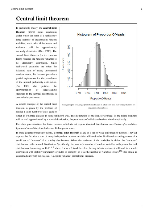
Central limit theoremHistogram plot of average proportion of heads in a fair coin toss, over a large number ofsequences of coin tosses In probability theory, the central limittheorem (CLT ) states conditionsunder which the mean of a sufficientlylarge number of independent randomvariables, each with finite mean andvariance, will be approximatelynormally distributed (Rice 1995). Thecentral limit theorem (in its commonform) requires the random variables tobe identically distributed. Sincereal-world quantities are often thebalanced sum of many unobservedrandom events, this theorem provides apartial explanation for the prevalenceof the normal probability distribution.The CLT also justifies theapproximation of large-samplestatistics to the normal distribution incontrolled experiments.A simple example of the central limit theorem is given by the problem ofrolling a large number of dice, each ofwhich is weighted unfairly in some unknown way. The distribution of the sum (or average) of the rolled numbers will be well approximated by a normal distribution, the parameters of which can be determined empirically.For other generalizations for finite variance which do not require identical distribution, see Lindeberg's condition ,Lyapunov's condition , Gnedenko and Kolmogorov states.In more general probability theory, a central limit theorem is any of a set of weak-convergence theories. They all express the fact that a sum of many independent random variables will tend to be distributed according to one of a small set of "attractor" (i.e. stable) distributions. When the variance of the variables is finite, the "attractor"distribution is the normal distribution. Specifically, the sum of a number of random variables with power law tail distributions decreasing as 1/|x |α + 1 where 0 < α < 2 (and therefore having infinite variance) will tend to a stable distribution with stability parameter (or index of stability) of α as the number of variables grows.[1] This article is concerned only with the classical (i.e. finite variance) central limit theorem.Classical central limit theoremA distribution being "smoothed out" by summation, showing original density of distribution and three subsequent summations; see Illustration of the central limit theoremfor further details.The central limit theorem is alsoknown as the second fundamentaltheorem of probability.[2] (The Law oflarge numbers is the first.)Let X 1, X 2, X 3, …, X n be a sequence ofn independent and identicallydistributed (iid) random variables eachhaving finite values of expectation µand variance σ2 > 0. The central limittheorem states that as the sample size nincreases, the distribution of thesample average of these randomvariables approaches the normaldistribution with a mean µ andvariance σ2/n irrespective of the shapeof the common distribution of theindividual terms X i .[3]For a more precise statement of thetheorem, let S n be the sum of the nrandom variables, given byThen, if we define new random variablesthen they will converge in distribution to the standard normal distribution N (0,1) as n approaches infinity. N (0,1) is thus the asymptotic distribution of the Z n's. This is often written asZ ncan also be expressed aswhereis the sample mean.Convergence in distribution means that, if Φ(z ) is the cumulative distribution function of N (0,1), then for every real number z, we haveorProofFor a theorem of such fundamental importance to statistics and applied probability, the central limit theorem has a remarkably simple proof using characteristic functions. It is similar to the proof of a (weak) law of large numbers. For any random variable, Y, with zero mean and unit variance (var(Y) = 1), the characteristic function of Y is, by Taylor's theorem,where o (t2 ) is "little o notation" for some function of t that goes to zero more rapidly than t2. Letting Yibe(Xi − μ)/σ, the standardized value of Xi, it is easy to see that the standardized mean of the observations X1, X2, ..., XnisBy simple properties of characteristic functions, the characteristic function of ZnisBut this limit is just the characteristic function of a standard normal distribution N(0, 1), and the central limit theorem follows from the Lévy continuity theorem, which confirms that the convergence of characteristic functions implies convergence in distribution.Convergence to the limitThe central limit theorem gives only an asymptotic distribution. As an approximation for a finite number of observations, it provides a reasonable approximation only when close to the peak of the normal distribution; it requires a very large number of observations to stretch into the tails.If the third central moment E((X1− μ)3) exists and is finite, then the above convergence is uniform and the speed of convergence is at least on the order of 1/n1/2 (see Berry-Esseen theorem).The convergence to the normal distribution is monotonic, in the sense that the entropy of Znincreases monotonically to that of the normal distribution, as proven in Artstein, Ball, Barthe and Naor (2004).The central limit theorem applies in particular to sums of independent and identically distributed discrete random variables. A sum of discrete random variables is still a discrete random variable, so that we are confronted with a sequence of discrete random variables whose cumulative probability distribution function converges towards a cumulative probability distribution function corresponding to a continuous variable (namely that of the normal distribution). This means that if we build a histogram of the realisations of the sum of n independent identical discrete variables, the curve that joins the centers of the upper faces of the rectangles forming the histogram converges toward a Gaussian curve as n approaches infinity. The binomial distribution article details such an application of the central limit theorem in the simple case of a discrete variable taking only two possible values.Relation to the law of large numbersThe law of large numbers as well as the central limit theorem are partial solutions to a general problem: "What is the limiting behavior of S n as n approaches infinity?" In mathematical analysis, asymptotic series are one of the most popular tools employed to approach such questions.Suppose we have an asymptotic expansion of ƒ(n ):Dividing both parts by φ1(n ) and taking the limit will produce a 1, the coefficient of the highest-order term in the expansion, which represents the rate at which ƒ(n ) changes in its leading term.Informally, one can say: "ƒ(n ) grows approximately as a 1 φ(n )". Taking the difference between ƒ(n ) and its approximation and then dividing by the next term in the expansion, we arrive at a more refined statement about ƒ(n ):Here one can say that the difference between the function and its approximation grows approximately as a 2 φ2(n ).The idea is that dividing the function by appropriate normalizing functions, and looking at the limiting behavior of the result, can tell us much about the limiting behavior of the original function itself.Informally, something along these lines is happening when the sum, S n , of independent identically distributed random variables, X 1, ..., X n , is studied in classical probability theory. If each X i has finite mean μ, then by the Law of Large Numbers, S n /n → μ.[4] If in addition each X i has finite variance σ2, then by the Central Limit Theorem,where ξ is distributed as N(0, σ2). This provides values of the first two constants in the informal expansionIn the case where the X i 's do not have finite mean or variance, convergence of the shifted and rescaled sum can also occur with different centering and scaling factors:or informallyDistributions Ξ which can arise in this way are called stable .[5] Clearly, the normal distribution is stable, but there are also other stable distributions, such as the Cauchy distribution, for which the mean or variance are not defined. The scaling factor b n may be proportional to n c , for any c ≥ 1/2; it may also be multiplied by a slowly varying function of n .[6] [7]The Law of the Iterated Logarithm tells us what is happening "in between" the Law of Large Numbers and the Central Limit Theorem. Specifically it says that the normalizing function intermediate in size between n of The Law of Large Numbers and √n of the central limit theorem provides a non-trivial limiting behavior.IllustrationGiven its importance to statistics, a number of papers and computer packages are available that demonstrate the convergence involved in the central limit theorem. [8]Alternative statements of the theoremDensity functionsThe density of the sum of two or more independent variables is the convolution of their densities (if these densities exist). Thus the central limit theorem can be interpreted as a statement about the properties of density functions under convolution: the convolution of a number of density functions tends to the normal density as the number of density functions increases without bound, under the conditions stated above.Characteristic functionsSince the characteristic function of a convolution is the product of the characteristic functions of the densities involved, the central limit theorem has yet another restatement: the product of the characteristic functions of a number of density functions becomes close to the characteristic function of the normal density as the number of density functions increases without bound, under the conditions stated above. However, to state this more precisely, an appropriate scaling factor needs to be applied to the argument of the characteristic function.An equivalent statement can be made about Fourier transforms, since the characteristic function is essentially a Fourier transform.Extensions to the theoremMultidimensional central limit theoremis an independent and We can easily extend proofs using characteristic functions for cases where each individual Xiidentically distributed random vector, with mean vector μ and covariance matrix Σ (amongst the individual components of the vector). Now, if we take the summations of these vectors as being done componentwise, then the Multidimensional central limit theorem states that when scaled, these converge to a multivariate normal distribution.Products of positive random variablesThe logarithm of a product is simply the sum of the logarithms of the factors. Therefore when the logarithm of a product of random variables that take only positive values approaches a normal distribution, the product itself approaches a log-normal distribution. Many physical quantities (especially mass or length, which are a matter of scale and cannot be negative) are the products of different random factors, so they follow a log-normal distribution. Whereas the central limit theorem for sums of random variables requires the condition of finite variance, the corresponding theorem for products requires the corresponding condition that the density function be square-integrable (see Rempala 2002).Lack of identical distributionThe central limit theorem also applies in the case of sequences that are not identically distributed, provided one of a number of conditions apply.Lyapunov conditionLet X n be a sequence of independent random variables defined on the same probability space. Assume that X n has finite expected value μn and finite standard deviation σn . We defineIf for some δ > 0, the expected values are finite for every i ∈ N and the Lyapunov's conditionis satisfied, then the distribution of the random variableconverges to the standard normal distribution N(0, 1).Lindeberg conditionIn the same setting and with the same notation as above, we can replace the Lyapunov condition with the following weaker one (from Lindeberg in 1920). For every ε > 0where 1{…} is the indicator function. Then the distribution of the standardized sum Z n converges towards the standard normal distribution N(0,1).Beyond the classical frameworkAsymptotic normality, that is, convergence to the normal distribution after appropriate shift and rescaling, is a phenomenon much more general than the classical framework treated above, namely, sums of independent random variables (or vectors). New frameworks are revealed from time to time; no single unifying framework is available for now.Under weak dependenceA useful generalization of a sequence of independent, identically distributed random variables is a mixing random process in discrete time; "mixing" means, roughly, that random variables temporally far apart from one another are nearly independent. Several kinds of mixing are used in ergodic theory and probability theory. See especially strong mixing (also called α-mixing) defined by α(n ) → 0 where α(n ) is so-called strong mixing coefficient.A simplified formulation of the central limit theorem under strong mixing is given in (Billingsley 1995, Theorem 27.4):Theorem. Suppose that X 1, X 2, … is stationary and α-mixing with αn = O (n −5) and that E(X n ) = 0 and E(X n 12) < ∞.Denote S n = X 1 + … + X n , then the limit σ2 = lim n n − 1E(S n 2) exists, and if σ ≠ 0 then converges in distribution to N(0, 1).In fact, σ2 = E(X 12) + 2∑k =1∞E(X 1X 1+k ), where the series converges absolutely.The assumption σ ≠ 0 cannot be omitted, since the asymptotic normality fails for X n = Y n − Y n −1 where Y n are another stationary sequence.For the theorem in full strength see (Durrett 1996, Sect. 7.7(c), Theorem (7.8)); the assumption E(X n 12) < ∞ is replaced with E(|X n |2 + δ) < ∞, and the assumption αn = O (n − 5) is replaced with Existence of such δ > 0 ensures the conclusion. For encyclopedic treatment of limit theorems under mixing conditions see (Bradley 2005).Martingale central limit theoremTheorem . Let a martingale M n satisfy •in probability as n tends to infinity,•for every ε > 0,as n tends to infinity,then converges in distribution to N(0,1) as n tends to infinity.See (Durrett 1996, Sect. 7.7, Theorem (7.4)) or (Billingsley 1995, Theorem 35.12).Caution: The restricted expectation E(X ; A ) should not be confused with the conditional expectation E(X |A ) = E(X ;A )/P (A ).Convex bodiesTheorem (Klartag 2007, Theorem 1.2). There exists a sequence εn ↓ 0 for which the following holds. Let n ≥ 1, and let random variables X 1, …, X n have a log-concave joint density f such that ƒ(x 1, …, x n ) = ƒ(|x 1|, …, |x n |) for all x 1, …,x n , and E(X k 2) = 1 for all k = 1, …, n . Then the distribution of is εn -close to N(0, 1) in the total variation distance.These two εn -close distributions have densities (in fact, log-concave densities), thus, the total variance distance between them is the integral of the absolute value of the difference between the densities. Convergence in total variation is stronger than weak convergence.An important example of a log-concave density is a function constant inside a given convex body and vanishing outside; it corresponds to the uniform distribution on the convex body, which explains the term "central limit theorem for convex bodies".Another example: ƒ(x 1, …, x n ) = const · exp ( − (|x 1|α + … + |x n |α)β) where α > 1 and αβ > 1. If β = 1 then ƒ(x 1, …,x n ) factorizes into const · exp ( − |x 1|α)…exp ( − |x n |α), which means independence of X 1, …, X n . In general,however, they are dependent.The condition ƒ(x 1, …, x n ) = ƒ(|x 1|, …, |x n |) ensures that X 1, …, X n are of zero mean and uncorrelated; still, they need not be independent, nor even pairwise independent. By the way, pairwise independence cannot replace independence in the classical central limit theorem (Durrett 1996, Section 2.4, Example 4.5).Here is a Berry-Esseen type result.Theorem (Klartag 2008, Theorem 1). Let X 1, …, X n satisfy the assumptions of the previous theorem, thenfor all a < b ; here C is a universal (absolute) constant. Moreover, for every c 1, …, c n ∈ R such that c 12 + … + c n 2 = 1,A more general case is treated in (Klartag 2007, Theorem 1.1). The condition ƒ(x1, …, xn) = ƒ(|x1|, …, |xn|) is replacedwith much weaker conditions: E(Xk ) = 0, E(Xk2) = 1, E(XkXℓ) = 0 for 1 ≤ k < ℓ≤ n. The distribution ofneed not be approximately normal (in fact, it can be uniform). However, the distributionof c1X1+ … + cnXnis close to N(0,1) (in the total variation distance) for most of vectors (c1, …, cn) according to theuniform distribution on the sphere c12 + … + cn2 = 1.Lacunary trigonometric seriesTheorem (Salem - Zygmund). Let U be a random variable distributed uniformly on (0, 2π), and Xk=r k cos(nkU + ak), where•nk satisfy the lacunarity condition: there exists q > 1 such that nk+1≥ qnkfor all k,•rkare such that•0 ≤ ak< 2π.Thenconverges in distribution to N(0, 1/2).See (Zygmund 1959, Sect. XVI.5, Theorem (5-5)) or (Gaposhkin 1966, Theorem 2.1.13). Gaussian polytopesTheorem (Barany & Vu 2007, Theorem 1.1). Let A1, ..., Anbe independent random points on the plane R2 eachhaving the two-dimensional standard normal distribution. Let Kn be the convex hull of these points, and Xnthe areaof KnThenconverges in distribution to N(0,1) as n tends to infinity.The same holds in all dimensions (2, 3, ...).The polytope Knis called Gaussian random polytope.A similar result holds for the number of vertices (of the Gaussian polytope), the number of edges, and in fact, faces of all dimensions (Barany & Vu 2007, Theorem 1.2).Linear functions of orthogonal matricesA linear function of a matrix M is a linear combination of its elements (with given coefficients), M↦ tr(AM) where A is the matrix of the coefficients; see Trace_(linear_algebra)#Inner product.A random orthogonal matrix is said to be distributed uniformly, if its distribution is the normalized Haar measure on the orthogonal group O(n,R); see Rotation matrix#Uniform random rotation matrices.Theorem (Meckes 2008). Let M be a random orthogonal n×n matrix distributed uniformly, and A a fixed n×n matrix such that tr(AA*) = n, and let X = tr(AM). Then the distribution of X is close to N(0,1) in the total variation metric uptoSubsequencesTheorem (Gaposhkin 1966, Sect. 1.5). Let random variables X 1, X 2, … ∈ L 2(Ω) be such that X n → 0 weakly in L 2(Ω) and X n 2 → 1 weakly in L 1(Ω). Then there exist integers n 1 < n 2 < … such thatconverges in distribution to N (0, 1) as k tends to infinity.Applications and examplesA histogram plot of monthly accidental deaths in the US, between 1973 and 1978 exhibitsnormality, due to the central limit theorem There are a number of useful and interesting examples and applicationsarising from the central limit theorem (Dinov, Christou & Sanchez2008). See e.g. [9], presented as part of the SOCR CLT Activity [10].•The probability distribution for total distance covered in a randomwalk (biased or unbiased) will tend toward a normal distribution.•Flipping a large number of coins will result in a normal distributionfor the total number of heads (or equivalently total number of tails).From another viewpoint, the central limit theorem explains thecommon appearance of the "Bell Curve" in density estimates applied toreal world data. In cases like electronic noise, examination grades, andso on, we can often regard a single measured value as the weightedaverage of a large number of small effects. Using generalisations of thecentral limit theorem, we can then see that this would often (though notalways) produce a final distribution that is approximately normal.In general, the more a measurement is like the sum of independent variables with equal influence on the result, the more normality it exhibits. This justifies the common use of this distribution to stand in for the effects of unobserved variables in models like the linear model.Signal processingSignals can be smoothed by applying a Gaussian filter, which is just the convolution of a signal with an appropriately scaled Gaussian function. Due to the central limit theorem this smoothing can be approximated by several filter steps that can be computed much faster, like the simple moving average.The central limit theorem implies that to achieve a Gaussian of variance σ2 n filters with windows of variances σ12,…, σn 2 with σ2 = σ12 + ⋯ + σn 2 must be applied.HistoryTijms (2004, p. 169) writes:“The central limit theorem has an interesting history. The first version of this theorem was postulated by the French-born mathematicianAbraham de Moivre who, in a remarkable article published in 1733, used the normal distribution to approximate the distribution of the number of heads resulting from many tosses of a fair coin. This finding was far ahead of its time, and was nearly forgotten until the famous French mathematician Pierre-Simon Laplace rescued it from obscurity in his monumental work Théorie Analytique des Probabilités , which waspublished in 1812. Laplace expanded De Moivre's finding by approximating the binomial distribution with the normal distribution. But as with De Moivre, Laplace's finding received little attention in his own time. It was not until the nineteenth century was at an end that the importance of the central limit theorem was discerned, when, in 1901, Russian mathematician Aleksandr Lyapunov defined it in general terms and proved precisely how it worked mathematically. Nowadays, the central limit theorem is considered to be the unofficial sovereign of probability theory.”Sir Francis Galton (Natural Inheritance , 1889) described the Central Limit Theorem as:“I know of scarcely anything so apt to impress the imagination as the wonderful form of cosmic order expressed by the "Law of Frequency of Error". The law would have been personified by the Greeks and deified, if they had known of it. It reigns with serenity and in complete self-effacement, amidst the wildest confusion. The huger the mob, and the greater the apparent anarchy, the more perfect is its sway. It is the supreme law of Unreason. Whenever a large sample of chaotic elements are taken in hand and marshaled in the order of their magnitude, an unsuspected and most beautiful form of regularity proves to have been latent all along.”The actual term "central limit theorem" (in German: "zentraler Grenzwertsatz") was first used by George Pólya in 1920 in the title of a paper.[11][12] Pólya referred to the theorem as "central" due to its importance in probability theory. According to Le Cam, the French school of probability interprets the word central in the sense that "it describes the behaviour of the centre of the distribution as opposed to its tails".[12] The abstract of the paper On the central limit theorem of calculus of probability and the problem of moments by Pólya[11] in 1920 translates as follows.“The occurrence of the Gaussian probability density e−x2 in repeated experiments, in errors of measurements, which result in the combination of very many and very small elementary errors, in diffusion processes etc., can be explained, as is well-known, by the very same limit theorem, which plays a central role in the calculus of probability. The actual discoverer of this limit theorem is to be named Laplace; it is likely that its rigorous proof was first given by Tschebyscheff and its sharpest formulation can be found, as far as I am aware of, in an article by Liapounoff. [...]”A thorough account of the theorem's history, detailing Laplace's foundational work, as well as Cauchy's, Bessel's and Poisson's contributions, is provided by Hald.[13] Two historical accounts, one covering the development from Laplace to Cauchy, the second the contributions by von Mises, Pólya, Lindeberg, Lévy, and Cramér during the 1920s, are given by Hans Fischer.[14][15] Le Cam describes a period around 1935.[12] See Bernstein (1945) for a historical discussion focusing on the work of Pafnuty Chebyshev and his students Andrey Markov and Aleksandr Lyapunov that led to the first proofs of the CLT in a general setting.A curious footnote to the history of the Central Limit Theorem is that a proof of a result similar to the 1922 Lindeberg CLT was the subject of Alan Turing's 1934 Fellowship Dissertation for King's College at the University of Cambridge. Only after submitting the work did Turing learn it had already been proved. Consequently, Turing's dissertation was never published.[16][17] .[18]Notes[1]Johannes Voit (2003), The Statistical Mechanics of Financial Markets (Texts and Monographs in Physics), Springer-Verlag, p. 124,ISBN 3-540-00978-7[2]p. 325, Introduction to probability, 2nd ed., Charles Miller Grinstead and James Laurie Snell, AMS Bookstore, 1997, ISBN 0821807498.[3]Theorem 27.1, p. 357, Probability and Measure, Patrick Billingsley, 3rd ed., Wiley, 1995, ISBN 0-471-00710-2.[4]Theorem 5.3.4, p. 47, A first look at rigorous probability theory, Jeffrey Seth Rosenthal, World Scientific, 2000, ISBN 9810243227.[5]p. 88, Information theory and the central limit theorem, Oliver Thomas Johnson, Imperial College Press, 2004, ISBN 1860944736.[6]pp. 61–62, Chance and stability: stable distributions and their applications, Vladimir V. Uchaikin and V. M. Zolotarev, VSP, 1999, ISBN9067643017.[7]Theorem 1.1, p. 8, Limit theorems for functionals of random walks, A. N. Borodin, Il'dar Abdulovich Ibragimov, and V. N. Sudakov, AMSBookstore, 1995, ISBN 0821804383.[8]Marasinghe, M., Meeker, W., Cook, D. & Shin, T.S.(1994 August), "Using graphics and simulation to teach statistical concepts", Paperpresented at the Annual meeting of the American Statistician Association, Toronto, Canada.[9]/socr/index.php/SOCR_EduMaterials_Activities_GCLT_Applications[10]/socr/index.php/SOCR_EduMaterials_Activities_GeneralCentralLimitTheorem[11]Pólya, George (1920), "Über den zentralen Grenzwertsatz der Wahrscheinlichkeitsrechnung und das Momentenproblem" (http://www-gdz.sub.uni-goettingen.de/cgi-bin/digbib.cgi?PPN266833020_0008) (in German), Mathematische Zeitschrift8: 171–181,doi:10.1007/BF01206525,[12](Le Cam 1986)[13]Hald, Andreas History of Mathematical Statistics from 1750 to 1930 (http://www.gbv.de/dms/goettingen/229762905.pdf), Ch.17.[14]Hans Fischer " The Central Limit Theorem from Laplace to Cauchy: Changes in Stochastic Objectives and in Analytical Methods" (http://www.ku-eichstaett.de/Fakultaeten/MGF/Mathematik/Didmath/Didmath.Fischer/HF_sections/content/1850.pdf) in Fischer (2010)[15]Hans Fischer "The Central Limit Theorem in the Twenties" (http://www.ku-eichstaett.de/Fakultaeten/MGF/Mathematik/Didmath/Didmath.Fischer/HF_sections/content/twenties_main.pdf) in Fischer (2010)[16]See Andrew Hodges(1983) Alan Turing: the enigma. London: Burnett Books., pp. 87-88.[17]Zabell, S.L., (2005) Symmetry and its discontents: essays on the history of inductive probability,Cambridge University Press. ISBN0521444705. (pp. 199 ff.)[18]See Section 3 of John Aldrich, "England and Continental Probability in the Inter-War Years", Journal Electronique d'Histoire desProbabilités et de la Statistique, vol. 5/2 Decembre 2009 (/decembre2009.html) Journal Electronique d'Histoire des Probabilités et de la Statistique.References•S. Artstein, K. Ball, F. Barthe and A. Naor (2004), "Solution of Shannon's Problem on the Monotonicity of Entropy" (/jams/2004-17-04/S0894-0347-04-00459-X/home.html), Journal of theAmerican Mathematical Society17, 975–982. Also author's site (http://www.math.tau.ac.il/~shiri/publications.html).•Barany, Imre; Vu, Van (2007), "Central limit theorems for Gaussian polytopes", The Annals of Probability (Institute of Mathematical Statistics) 35 (4): 1593–1621, doi:10.1214/009117906000000791. Also arXiv (http:// /abs/math/0610192).•S.N.Bernstein, On the work of P.L.Chebyshev in Probability Theory, Nauchnoe Nasledie P.L.Chebysheva.Vypusk Pervyi: Matematika. (Russian) [The Scientific Legacy of P. L. Chebyshev. First Part: Mathematics] Edited by S. N. Bernstein.] Academiya Nauk SSSR, Moscow-Leningrad, 1945. 174 pp.•Billingsley, Patrick (1995), Probability and Measure (Third ed.), John Wiley & sons, ISBN 0-471-00710-2•Bradley, Richard (2007), Introduction to Strong Mixing Conditions (First ed.), Heber City, UT: Kendrick Press, ISBN 097404279X•Dinov, Ivo; Christou, Nicolas; Sanchez, Juana (2008), "Central Limit Theorem: New SOCR Applet and Demonstration Activity", Journal of Statistics Education (ASA) 16 (2). Also at ASA/JSE (http://www.amstat.org/publications/jse/v16n2/dinov.html).•Durrett, Richard (1996), Probability: theory and examples (Second ed.)•Fischer, H. (2010) A History of the Central Limit Theorem: From Classical to Modern Probability Theory, Springer. ISBN 0387878564•Gaposhkin, V.F. (1966), "Lacunary series and independent functions", Russian Math. Surveys21 (6): 1–82, doi:10.1070/RM1966v021n06ABEH001196.•Klartag, Bo'az (2007), "A central limit theorem for convex sets", Inventiones Mathematicae168, 91–131.doi:10.1007/s00222-006-0028-8 Also arXiv (/abs/math/0605014).•Klartag, Bo'az (2008), "A Berry-Esseen type inequality for convex bodies with an unconditional basis", Probability Theory and Related Fields. doi:10.1007/s00440-008-0158-6 Also arXiv (/abs/0705.0832).•Le Cam, Lucien (1986), "The central limit theorem around 1935" (/euclid.ss/ 1177013818), Statistical Science1:1, 78–91.•Meckes, Elizabeth (2008), "Linear functions on the classical matrix groups", Transactions of the American Mathematical Society360: 5355–5366, doi:10.1090/S0002-9947-08-04444-9. Also arXiv (/abs/ math/0509441).•Rempala, G. and J. Wesolowski, (2002) "Asymptotics of products of sums and U-statistics" (http://www.math./~ejpecp/EcpVol7/paper5.pdf), Electronic Communications in Probability, 7, 47–54.•Rice, John (1995), Mathematical Statistics and Data Analysis (Second ed.), Duxbury Press, ISBN 0-534-20934-3•Tijms, Henk (2004) Understanding Probability: Chance Rules in Everyday Life (/dp/ 0521540364/), Cambridge: Cambridge University Press. ISBN 0521540364•Zygmund, Antoni (1959), Trigonometric series, Volume II, Cambridge. (2003 combined volume I,II: ISBN 0521890535)。
美国标准中的地震动参数概念(中英文对照)

Design earthquakes. The design earthquakes for hydraulic structures are the OBE and the MDE.设计地震:水工结构的设计地震有OBE和MDE,即运行基准地震和最大设计地震。
The actual levels of ground motions for these earthquakes depend on the type of hydraulic structure under consideration, and are specified in the seismic design guidance provided for a particular structure in conjunction with ER 1110-2-1806.地震动参数的实际取值跟水工建筑物的类型有关,具体可参照ER 1110-2-1806。
(1) Operating basis earthquake (OBE). The OBE is an earthquake that can reasonably be expected to occur within the service life of the project, that is, with a 50 percent probability of exceedance during the service life. The associated performance requirement is that the project function with little or no damage, and without interruption of function.运行基准地震(OBE):OBE是指在工程的服务生命周期中可能合理预期发生的地震,即在工程生命周期中超过50%的发生概率,在该地震作用下,工程的相关性能要求几乎没有或没有破坏,工程的相关功能没有中断。
棣莫弗-拉普拉斯中心极限定理的英文
棣莫弗-拉普拉斯中心极限定理的英文全文共四篇示例,供读者参考第一篇示例:The Central Limit Theorem (CLT) is a fundamental concept in the field of statistics that was first formulated by Pierre-Simon Laplace in the late 18th century. The theorem states that the distribution of the sum (or average) of a large number of independent and identically distributed random variables approaches a normal distribution regardless of the shape of the original distribution.第二篇示例:The Central Limit Theorem (CLT) is a fundamental concept in statistics and probability theory. It states that the distribution of the sum (or average) of a large number of independent, identically distributed random variables approaches a normal distribution, regardless of the original distribution of the variables. One of the most famous versions of this theorem is the De Moivre-Laplace Central Limit Theorem, named after two prominent mathematicians, Abraham de Moivre andPierre-Simon Laplace.第三篇示例:The central limit theorem (CLT) is a fundamental theorem in probability theory and statistics that states that the distribution of the sum (or average) of a large number of independent, identically distributed random variables approaches a normal distribution, regardless of the shape of the original distribution. This theorem has profound implications in various fields such as finance, engineering, and biology, where it allows researchers to make reliable predictions even when they have limited information about the underlying data.第四篇示例:The Central Limit Theorem, also known as the DeMoivre-Laplace Theorem, is a fundamental concept in probability theory and statistics. It states that the sum of a large number of independent and identically distributed random variables will be approximately normally distributed, regardless of the distribution of the original variables.。
广义中心极限定理 英语
广义中心极限定理英语The Generalized Central Limit TheoremThe central limit theorem is a fundamental concept in probability theory and statistics, which states that the distribution of the sum or average of a large number of independent and identically distributed random variables will tend to a normal distribution, regardless of the underlying distribution of the individual variables. This theorem has far-reaching implications in various fields, including finance, engineering, and the social sciences.While the classical central limit theorem is a powerful tool, it is limited to the case where the random variables are independent and identically distributed. However, in many real-world situations, this assumption may not hold, and the variables may exhibit more complex dependencies or non-identical distributions. This is where the generalized central limit theorem (GCLT) comes into play.The GCLT is a more general version of the central limit theorem that relaxes the assumptions of independence and identical distribution. It states that the distribution of the sum or average of a large number of random variables will converge to a stable distribution,which is a broader class of probability distributions that includes the normal distribution as a special case.The key to understanding the GCLT is the concept of a stable distribution. A stable distribution is a probability distribution that satisfies the following property: the sum of two independent random variables with the same stable distribution is also a random variable with the same stable distribution, up to a scale and location parameter. This property is known as the stability property, and it is the foundation of the GCLT.There are four main parameters that characterize a stable distribution: the index of stability (α), the skewness parameter (β), the scale parameter (σ), and the location parameter (μ). The index of stability, α, is the most important parameter, as it determines the shape of the distribution. When α = 2, the stable distribution reduces to the normal distribution, which is the special case covered by the classical central limit theorem.The GCLT states that if the sum or average of a large number of random variables is properly normalized, then the distribution of the normalized sum or average will converge to a stable distribution as the number of variables goes to infinity. The specific form of the stable distribution depends on the values of the four parameters mentioned above, which in turn depend on the characteristics of theindividual random variables.One of the key advantages of the GCLT is its ability to handle non-independent and non-identically distributed random variables. This is particularly important in many real-world applications, where the assumptions of independence and identical distribution may not be realistic. For example, in financial markets, asset returns often exhibit complex dependencies and non-normal distributions, which can be better captured by the GCLT.Another important aspect of the GCLT is its connection to the concept of heavy-tailed distributions. Heavy-tailed distributions are probability distributions that have a slower decay rate in their tails compared to the normal distribution. These distributions are often observed in various natural and social phenomena, such as the distribution of wealth, the size of earthquakes, and the intensity of internet traffic. The GCLT provides a theoretical framework for understanding the emergence of heavy-tailed distributions in the sum or average of a large number of random variables.In conclusion, the generalized central limit theorem is a powerful and versatile tool in probability theory and statistics. It extends the classical central limit theorem to a broader class of random variables, allowing for more realistic modeling of complex real-world phenomena. The GCLT has important applications in fields such asfinance, engineering, and the social sciences, and its continued study and development is an active area of research.。
Central limit theorem, deformed exponentials and superstatistics

a r X i v :0706.0151v 1 [c o n d -m a t .s t a t -m e c h ] 1 J u n 2007Central limit theorem,deformed exponentials and superstatisticsC.Vignat 1and A.Plastino 2∗1L.T.H.I.,E.P .F .L.,Lausanne,Switzerland and2Facultad de Ciencias Exactas,Universidad Nacional de La Plata and CONICET,C.C.727,1900La Plata,Argentina†AbstractWe show that there exists a very natural,superstatistics-linked extension of the central limit theorem (CLT)to deformed exponentials (also called q-Gaussians):This generalization favorably compares with the one provided by S.Umarov and C.Tsallis [arXiv:cond-mat/0703533],since the latter requires a special ”q-independence”condition on the data.On the contrary,our CLT proposal applies exactly in the usual conditions in which the classical CLT is used.Moreover,we show that,asymptotically,the q-independence condition is naturally induced by our version of the CLT.I.INTRODUCTIONThe central limit theorems(CLT)can be ranked among the most important theorems in prob-ability theory and statistics and plays an essential role in several basic and applied disciplines, notably in statistical mechanics.Pioneers like A.de Moivre,P.S.de Laplace,S.D.Poisson,and C.F.Gauss have shown that the Gaussian function is the attractor of independent additive contri-butions with afinite second variance.Distinguished authors like Chebyshev,Markov,Liapounov, Feller,Lindeberg and L´e vy have also made essential contributions to the CLT-theory.The random variables to which the classical CLT refers are required to be independent.Sub-sequent efforts along CLT lines have established corresponding theorems for weakly dependent random variables as well(see some pertinent references in[1,2,3]).However,the CLT does not hold if correlations between far-ranging random variables are not negligible(see[4]).Recent developments in statistical mechanics that have attracted the attention of many re-searches deal with strongly correlated random variables([5]and references therein).These cor-relations do not rapidly decrease with any increasing distance between random variables and are often referred to as global correlations(see[6]for a definition).Is there an attractor that would replace the Gaussians in such a case?The answer is in the affirmative,as shown in[1,2,3],with the deformed or q-Gaussian playing the starring role.It is asserted in[2]that such a theorem cannot be obtained if we rely on classic algebra:it needs a construction based on a special algebra,which is called q-algebra[15].The goal of this communication is to show that a q-generalization of the central limit theorem becomes indeed possible and in a very simple way without recourse to q-algebra.A.Systems that are q-distributedConsider a system S described by a random vector X with d−components whose covariance matrix readsK= XX t ≡EXX t,(1) the superscript t indicating transposition.We say that X is q−Gaussian(or deformed Gaussian-) distributed if its probability distribution function writes as described by Eqs.(2)-(3)below.•in the case1<q<d+4q−1 q−1−d 1−q,(2)with matrixΛbeing related to K in the fashionΛ=(m−2)K.(3) The number of degrees of freedom m is defined in terms of the dimension d of X as[7]m=2q−1+dΓ 2−q1−q+,(5) where the matrixΣis related to the covariance matrix viaΣ=pK.We introduce here a parameter p defined asp=22−q√|2πK|1/2t1−∞... t d−∞e−X t K−1XThe basic idea leading towards non-conventional CLTs is tofind conditions under which con-vergence to the usual normal cumulative density function(cdf)Φ1with covariance matrix K can be replaced by convergence to a q−Gaussian cdfΦq(t)= t1−∞... t d−∞f X,q(x)dx1...dx d(9) with q>1,f X,q as defined in(2)and parameter m defined by(4)or,for q<1,Φq(t)= t1−∞... t d−∞f X,q(x)dx1...dx d(10) with f X,q as defined in(5)and parameter p defined by(6).We note that both cases m→+∞and p→+∞correspond to convergence q→1to the Gaussian case.In two recent contributions,S.Umarov and C.Tsallis highlight the existence of such a central limit theorem,in the univariate[2]and multivariate[1]case,provided there exists a certain kind of dependence,called q−independence,between random vectors X i.This q−independence con-dition is expressed in terms of the notions of q−Fourier transform F q and of q−product⊗q[1,2] asF q[X1+X2]=F q[X1]⊗q F q[X2]which reduces to conventional independence for q=1.We recall that the q−product of x∈C and y∈C isx⊗q y= x1−q+y1−q−1 11−q dx.However,this approach suffers from the lack of physical interpretation for such special depen-dence;moreover,the q−Fourier transform is a nonlinear transform(unless q=1)what makes its use rather difficult.Another approach,as described in[8],consists in keeping the independence assumption be-tween vectors X i while replacing the n terms in(7)by a random number N(n)of terms.That is, if the random variable N(n)follows a negative binomial distribution so as to diverge in a specified way,then convergence to a q−Gaussian distribution occurs whenever convergence occurs in the usual sense.In the present contribution we show that there exists a much more natural way to extend the CLT,based on the Beck-Cohen notion of superstatistics[9](see the discussion in[10]).Our starting point is the same as that in Umarov’s approach(i.e.,assuming some kind of dependence between the summed terms).However,the manner in which we introduce this dependence among data is a natural one that can be interpreted in the physical framework of the Cohen-Beck physics (see[14]for an interesting overview).III.PRESENT RESULTSOur present results can be conveniently condensed by stating two theorems,according to the value of parameter q.The essential idea is that of suitably introducing a chi-distributed random variable a that is independent(case q>1)or dependent(case q<1)of the data X i,and then constructing the following scale mixture(typical of superstatistics[10])Z n=1nni=1X i.(11)A.The case q>1Theorem2.If X1,X2,...are i.i.d.random vectors in R d with zero mean and covariance ma-trix K,and if a denotes a random variable chi-distributed with m degrees of freedom,scale parameter(m−2)−1/2,and chosen independent of the X i,then random vectorsZ n=1nni=1X i(12)converge weakly to a multivariate q−Gaussian vector Z with covariance matrix K.Equivalently stated:∀t∈R d,limn→+∞Pr{Z n≤t}=Φq(t);(13) with cdfΦq(t)defined as in(9).Moreover,q=m+d+2√2(m−2)mΓm2.Now,by the multivariate central limit theorem1above[17]1 nn i=1X i⇒Nwhere N is a normal vector in R d with covariance matrix K.Applying from[11]its result[Th.2.8]we deduce thatZ n⇒Nafollows a q-Gaussian distribution with covariance matrix K and parameter q defined by (4).B.The case q<1The extension of theorem2to the case q<1proceeds as follows.Theorem3.If X1,X2,...are i.i.d.random vectors in R d with zero mean and covariance matrix K,and if a is a random variable independent of the X i that is chi-distributed with m degrees of freedom and scale parameter√b√a2+ 1n n i=1X i tΛ−1 1n n i=1X i (16) converge weakly to a multivariate q−Gaussian vector Y with covariance matrix K and distribu-tion function given by(9).Moreover,q=m−4√Remark1.We note that Y n in(15)is a normalized version of Z n in(12);however,thefluctuation term a is replaced by afluctuation termb= √√d.Consider n=n0+n1together with the division of sum Z n in(12)into two parts asZ n=1n n0 i=1X i+n i=n0+1X i=Z(1)n+Z(2)n.(18)Assume that the characteristic functionφof X i is such that R d|φ|νdt<∞for someν≥1,and that data X i are symmetric(X i and−X i have the same distribution).Then random vectors Z(1)n and Z(2)n are asymptotically q−independent in the sense that∀ǫ>0,∃N such that n0>N,n1>N⇒||F q[Z(1)n+Z(2)n]−F q[Z(1)n]⊗q1F q[Z(2)n]||∞<ǫwith q1=z(q)=2q+d(1−q)IV.PROOF OF THE LINKING THEOREMA.IntroductionIn order to simplify the proof we will assume that vectors X i verify a stronger version of the CLT than the one stated in theorem1,namely the CLT in total variation.Now,the total variation divergence between two probability densities f and g is1d T V(f,g)=√√a•step 2:let us fix ǫ>0,and writeF q [Z (1)n +Z (2)n ]−F q [Z (1)n ]⊗q 1F q [Z (2)n ] ∞≤ F q [Z (1)n +Z (2)n ]−F q [˜Z (1)n +˜Z (2)n ] ∞+ F q [˜Z (1)n ]⊗q 1F q [˜Z (2)n ]−F q [Z (1)n ]⊗q 1F q [Z (2)n ] ∞•step 3:the first term F q [Z (1)n +Z (2)n ]−F q [˜Z (1)n +˜Z (2)n ] ∞= F q [Z n ]−F q [˜Zn ] ∞can be bounded as followsF q [Z n ]−F q [˜Zn ] ∞≤2d T V (Z n ,˜Z n )≤2d T V (X n ,˜X n )where the first inequality follows from Lemma 3and the second one from Lemma 1below.Thus a value N 1can be chosen so that n 0>N 1and n 1>N 1ensure that this term is smaller thanǫ4.•step 5:The consideration of N =max(N 1,N 2,N 3)is then seen to prove the linking theorem 4We turn now our attention to those results that we have used in this proof.ponents of q −Gaussian vectors are q −independentWe first begin to check that “sub-vectors”extracted from q −Gaussian vectors are exactly q −independent;this results is obvious from the fact that,by the CLT given in [1](Thm. 4.1),these sub-vectors can be considered as limit cases of sequences of q −independent sequences.However,the mathematical verification of this property is of an instructive nature and we proceed to give it.For readability,we will say that X ∼(q,d )if X is a q −Gaussian vector of dimension d and nonextensivity parameter q.Theorem6.If1<q0<1+2>1and q1=z(q)>1.2+d(1−q0)Proof.Since X1∼(q,d),we know from the Corollary2.3of[1]that F q[X1]∼(q1,d).Moreover, since X1and X2are components of the same q−Gaussian vector,from[8]we deduce that X1+ X2∼(q,d)so that F q[X1+X2]∼(q1,d).Finally,it is easy to check that since F q[X1]∼(q1,d) and F q[X2]∼(q1,d)then F q[X1]⊗qF q[X2]∼(q1,d).The fact that both terms have same1covariance matrices is straightforward,what proves the result.We note that q−correlation(21)corresponds to q−independence of the third kind as listed in Table1of[1].We pass now to the consideration of the four Lemmas invoked in the proof of the linking theorem.C.Technical lemmasAs we are concerned with scale mixtures of Gaussian vectors,we need the following lemma. Lemma1.If U and V are random vectors in R d and a is a random variable independent of U and V thend T V U a ≤d T V(U,V).(22) Proof.The distributions of scale mixtures U/a and V/a write,in terms of the distributions of U and of V,in the fashionf U/a(x)= R+1a da,g V/a(x)= R+1a da.(23)It thus follows thatd T V U a =12 R d| R+1a −f V x2 R d R+1a −f V x2 R+12R+f a(a)da R d|f U(z)−f V(z)|dz=11−qis a Lipschitz function with unit constant:|ψq,z(x1)−ψq,z(x0)|≤|x1−x0|,(24) Proof.We have|ψq,z(x1)−ψq,z(x0)|≤supx0≤x≤x1|ψ′q,z(x)||x1−x0|,(25)whereψ′q,z(x)=1q−1,(26)with q|1+zx q−1|qLemma3.For any random vectors U and V,if q≥1,the following inequality holdsF q[U]−F q[V] ∞≤2d T V(U,V).(28) Proof.This result is a straightforward consequence of inequality(34)of reference[1].However, an elementary proof writes as follows:denote f U and f V the respective probability densities of U and V.Then,∀ξ∈R d,|F q[U](ξ)−F q[V](ξ)|≤ R d| f1−q U(x)+(1−q)ix tξ 11−q|dxAsℜ((1−q)ix tξ)=0and f U≥0,by lemma2,the integrand is bounded by|f U(x)−f V(x)|; since this holds∀ξ∈R d,the desired result follows.We remark here that inequality(28)is a simple generalization of the well-known q=1case, in which F q=1corresponds to the classical Fourier transform.Thus a well-known result of the Fourier theory is reproduced,namelyF1[U]−F1[V] ∞≤2d T V(U,V).As another consequence of lemma2we haveLemma4.For notational simplicity,let us denote as Z1=Z(1)n,Z2=Z(2)n,˜Z1=˜Z(1)n and˜Z2=˜Z(2)n those random vectors defined in part IV.A.Then,for n large enough,F q[Z1](ξ)⊗q1F q[Z2](ξ)−F q[˜Z1](ξ)⊗q1F q[˜Z2](ξ) ∞≤2d T V(Z1,˜Z1)+2d T V(Z2,˜Z2). Proof.For anyξ∈R d,|F q[Z1](ξ)⊗q1F q[Z2](ξ)−F q[˜Z1](ξ)⊗q1F q[˜Z2](ξ)|≤|F q[Z1](ξ)⊗q1F q[Z2](ξ)−F q[˜Z1](ξ)⊗q1F q[Z2](ξ)|+|F q[˜Z1](ξ)⊗q1F q[Z2](ξ)−F q[˜Z1](ξ)⊗q1F q[˜Z2](ξ)|=|ψq1,F1−q1q[Z2](ξ)−1(F q[Z1](ξ))−ψq1,F1−q1q[Z2](ξ)−1(F q[˜Z1](ξ))|+|ψq1,F1−q1q[˜Z1](ξ)−1(F q[Z2](ξ))−ψq1,F1−q1q[˜Z1](ξ)−1(F q[˜Z2](ξ))|Since˜Z2is q−Gaussian,and since1<q<1+20,it follows that F1−q1[˜Z2](ξ)≥1.From the CLT in total variation,we can choose n large qenough so that d T V(F q[Z2],F q[˜Z2])is arbitrarily small,which in turns implies,by Lemma3,that |F q[Z2](ξ)−F q[˜Z2](ξ)|is arbitrarily small as well.By continuity of the function x→x1−q1−1,[Z2](ξ)−1≥0. and since F q[Z2]is real-valued by the symmetry of the data,this ensures that F1−q1qThus,thefirst term can be bounded using lemma2in the fashion|ψq1,F1−q1q[Z2](ξ)−1(F q[Z1](ξ))−ψq1,F1−q1q[Z2](ξ)−1(F q[˜Z1](ξ))|≤|F q[˜Z1](ξ)−F q[Z1](ξ)|. Accordingly,since˜Z1is q−Gaussian,there existsα1≥0such that F1−q1q[˜Z1](ξ)−1=α1(q1−1)ξ2,hence F1−q1[˜Z1](ξ)≥1.Recourse again to lemma2yieldsq|ψq1,F1−q1q[˜Z1](ξ)−1(F q[Z2](ξ))−ψq1,F1−q1q[˜Z1](ξ)−1(F q[˜Z2](ξ))|≤|F q[˜Z2](ξ)−F q[Z2](ξ)|. Applying now lemma3to each of both terms above yields|F q[Z1](ξ)⊗q1F q[Z2](ξ)−F q[˜Z1](ξ)⊗q1F q[˜Z2](ξ)|≤2d T V(Z1,˜Z1)+2d T V(Z2,˜Z2).As this holds for any value ofξ∈C,the result follows.V.CONCLUSIONSWe have here dealt with non-conventional central limit theorems,whose attractor is a deformed or q-Gaussian.Based on the Beck-Cohen notion of superstatistics[9],with scale mixtures relating random variables`a la Eq.(11),it has been shown that there exists a very natural extension of the central limit theorem to these deformed exponentials that quite favorably compares with the one provided by S.Umarov and C.Tsallis[arXiv:cond-mat/0703533].This is so because the latter re-quires a special“q-independence condition on the data”.On the contrary,our CLT proposal applies exactly in the usual conditions in which the classical CLT is used.However,links between ours and the Umarov-Tsallis treatment have also been established,which makes the here reported CLT a hopefully convenient tool for understanding the intricacies of the physical processes described by power-laws probability distributions,as exemplified,for instance,by the examples reported in [5](and references therein).[1]S.Umarov and C.Tsallis,[arXiv:cond-mat/0703533].[2]S.Umarov,S.Steinberg,C.Tsallis,[arXiv:condmat/0603593].[3]S.Umarov,S.Steinberg,C.Tsallis,[arXiv:condmat/0606040]and[arXiv:condmat/0606038](2006).[4]H.G.Dehling,T.Mikosch,M.Sorensen(editors),Empirical process techniques for dependent data(Birkhaeser,Boston-Basel-Berlin,2002).[5]Among literally hundreds of references see,for instance,M.Gell-Mann and C.Tsallis,Eds.Nonex-tensive Entropy:Interdisciplinary applications(Oxford University Press,Oxford,2004);A.Plastino and A.R.Plastino,Braz.J.of Phys.,29(1999)50;C.Vignat,A.Plastino,Phys.Lett.A365(2007) 370.[6] C.Tsallis,M.Gell-Mann,and Y.Sato,A102(2005)15377.[7] C.Vignat,A.Plastino,Physics Letters A343(2005)411.[8] C.Vignat and A.Plastino,Phys.Lett.A360(2007)415.[9] C.Beck and E.G.D.Cohen,Physica A322(2003)267.[10] C.Vignat,A.Plastino,and A.R.Plastino,Il Nuovo Cimento B120(2005)951.[11]P.Billingsley,Convergence of Probability Measures,Second Edition,Wiley Series in Probability andStatistics,1999.[12] A.W.van der Vaart,Asymptotic Statistics(Cambridge Series in Statistical and Probabilistic Mathe-matics,1998).[13]V.Kac and P.Cheung,Quantum Calculus,Springer,2001[14] C.Beck,Superstatistics:theoretical concepts and physical applications,arXiv:cond-mat.stat-mech/07053832v1,2007[15]This should not be confused with quantum algebra as defined in[13][16]Note that inequality between vectors W n≤t denotes the set of d component-wise inequalities{W n(k)≤t k;1≤k≤d}.[17]note that,below,symbol⇒denotes weak convergence。
4. Central Limit Theorem
Sampling Distribution of Sample MeansA sampling distribution of sampling means is a distribution obtained by using the means computed from random samples of a specific size taken from a population.Sampling ErrorSampling error is the difference between the sample measures and the corresponding population measure due to the fact that the sample is not a perfect representation of the population.Properties of the Distribution of Saample Mean1.The mean of the sample means will be the same as the population mean.2.The standard deviation of the sample means will be smaller than the standard deviation of the population, and it will be equal to the population standard deviation, divided by the square root of the sample size.Formula1.μμμμ==∑=X X n X2.n X σσ=The Central Limit TheoremAs the sample size n increases, the shape of the distribution of the sample means taken from a population with mean μand standard deviation σwill approach a normal distribution. This distribution will have mean μand a standard deviationn σ. The z-values are computed as : n X z /σμ-=Finite Population Correction FactorSince most samples are drawn without replacement from a finite population, a correction factor is used.1--N nNWhen the sample size n is greater than 5% of thepopulation size N, the finite correction factor is used to correct the standard error of the mean.1--⋅=N n N nX σσ The formula for computing the z-value is:1--⋅-=N n N nX z σμThe Normal Approximation To The Binomial DistributionCondition: 5≥np and 5≥nqA correction for continuity is a correction employed when a continuous distribution is used toapproximate a discrete distribution.()()()()()()()()5.455.775.085.0885.05.0≥=≥≤=≤+≤≤-==+≤≤-=X NP X BP X NP X BP X NP X BP k X k NP k BPProcedure for the Normal Approximation to theBinomial Distribution1.Check to see whether the normal approximation can be used.2.Find the mean npμand the standard deviation npq.=3.Write the problem in probability notation, using X.4.Rewrite the problem by using the continuity correction factor, and show the corresponding area under the normal distribution.5.Find the corresponding z-values.6.Find the solution.。
陶哲轩评述佩雷尔曼的庞加莱猜想证明

1This hypothesis is in fact quite natural, because the arguments also show conversely that finite time extinction for Ricci flow is only possible when the fundamental group is a free product of finite groups and infinite simple groups. For the purposes of proving just the Poincar´e conjecture, though, it is possible to work entirely in the category of simply connected manifolds throughout, although this only simplifies the argument at one small point (in the proof of finite time extinction). We thank John Morgan for clarifying this point.
Lec_14
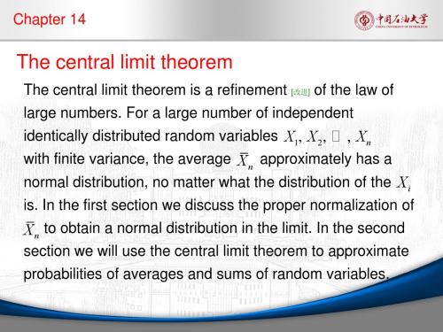
14.1 Standardizing averages
In case X1, X2 , … are independent N m, s 2 distributed
random variables, we know from Section 11.2 and the rule on expectation and variance under change of units, that Z n has an N ( 0, 1) distribution for all n. For the gamma and bimodal random variables from Section 13.1 we depicted[描画]
14.1 Standardizing averages In the previous chapter we saw that the law of large numbers guarantees the convergence to μ of the average X n of n independent random variables X1, X2 , … , Xn , all having
+ a[i] = mean(x) } > hist(a, freq=FALSE, ylim=c(0, 6)) > lines(density(a), col="blue") > curve(dnorm(x, mean(a), sd(a)), 3.2, 3.8, add=T, lty=2, col=2)
the same expectation μ and variance s 2. This convergence
was illustrated by Figure 13.1.
肖仰华_大数据时代的人工智能与智能医疗

大数据人工智能的机遇中国医疗现状的问题智能医疗的实现路径大数据人工智能技术的挑战问题信任均衡多因素医生病人医院社会精准医疗面临的挑战足够的资源病理学家的匮乏超负荷工作大量的各类数据我们正在经历!终极目标将答案交给机器:海量数据作为学习样本,不断优化模型贴近答案代表:基于深度学习的系统将目标交给机器:机器拥有自我学习,自我完善的能力,写出能够完善自身的代码,不断从开放世界获取信息并改造自身。
早期人工智能将规则交给机器:给定规则,机器根据规则作出相应判断代表:规则系统和专家系统完整生态深度学习模型:具有较深层次的神经网络模拟人脑的深度结构;模仿人类逐层进行,逐步抽象的认知过程使得类人学习成为可能无需传统机器学习的专家特征定义是一种大规模语义网络,表达了实体/概念及其之间的各类语义关系海量规模、语义丰富、结构友好为语义理解提供丰富的背景知识是能够满足机器认知需求的知识表示路径1.Understands natural language and human communicationcognitive services •Ask 智慧搜索智能推荐精准画像自然交互论坛十亿级文献一亿级病例百万级自然语言文本杂志/论文/指南/书籍医学领域知识库自然语言问答病症搜索推荐诊断搜索推荐构建用药搜索推荐疾病症状用药诊断病例大数据案例支撑分类归档支撑病例数据挖掘n语言是人类思维的工具n语言认知能力是人类作为万物之灵的根本能力机器语言认知是实现类人智能的关键机器能够理解人类语言么?•Ambiguous contextual implicithuman cognitioninfinitePart of materialsare from‘Watson System’by Devendra Chaplot et al.Conceptulization (概念化)Association (联想)Categorization (范畴化)Metaphor (隐喻理解)Frame (场景理解)Induction (归纳)Inference (推理)Xiangyan Sun, et al, Syntactic Parsing of WebQueries.(submitted to EMNLP 2016)Example :cover iphone 6 plus àcoveriphone 6 plus cover àcover576577578579580581582583584585586587588589590591592593594EMNLP 2016Submission ***.Confidential review copy.DO NOT DISQueryParserStanford parsertoys kids NNS NNSnnkids toys NNS NNSnn toys kids NNS NNSnnkids toys NNS NNSnnvanguard school lake wales NN NN NN NNSnnnnnn vanguard school lake wales NN NN NN NNSnnnnnnpretty little liars season 4episode 6RB JJ NNS NN CD NN CD advmod nnnn numnn numpretty little liars season 4episode 6RB JJ NNS NN CD NN CDadvmodnnnn numnnnuminterview questions contract specialistNN NNS NN NNnnnnnncontract specialist interview questionNN NN NN NNnnnnnninterview questions contract specialistNN NNS NN NNnnnnnncontract specialist interview questionNN NN NN NNnnnnnnTable 4:Case study of parsers.5.1Case Study5.3Web Query TreeWe evaluate the 3steps ter each step,we sampl and manually compute We also count the numb each step.The results a•Inferring a depen sentence)pair,w the sentence to th stances shown in ber of (query,sen we obtain depende queries,while the ing criterion.Thi By sacrificing rec high precision.G precision is more•Inferring a uniqu问题:Given words, can we inference the concept these words are talking about?Conceptulization(概念化) Association(联想)Categorization(范畴化)Metaphor(隐喻理解)Frame(场景理解)Induction(归纳) Inference(推理)问题:Find the related entity to complete a minimum conceptExample:baidu, ali->tencentBecause they all belong to concept BAT)Yi Zhang, et al, Entity suggestion with conceptual explanation, (submitted to ICDE2017)Conceptulization (概念化)Association (联想)Categorization (范畴化)Metaphor (隐喻理解)Frame (场景理解)Induction (归纳)Inference (推理)Example :Sex=man,Marriage status=unmarried àBachelorrich property-value information for entities only.Inferencing DFs of categories from their entities is not easy.In the tra-ditional efforts,psychologists manually construct DFs for a very limited number of popular categories,such as birds ,an-imals ,and cars [Collins and Quillian,1969;Tulving,1972;Smith et al.,1974].However,it is impractical to find the DFs for millions of categories in the real world manually,es-pecially considering that there are millions of tail categories which are unfamiliar to most of us.ANIMAL BIRD OWL [Multicellular, Eukaryotic, Kingdom Animalia][Order Strigiform][feathered, winged, bipedal, warm-blooded,egg-laying, vertebrate]ROBIN FISHSHARKisA isAisA isA isA [red-breast]Figure 1:An example of DFs of categories.The goal of this paper thus is to automatically find defin-ing features for millions of categories in the real world.define a category.For films directedpher Nolan ,we use its basic type film as Feature Mining our solution framework,then elaborate each framework.orkFramework of Defining Feature Mining.a bootstrapping approach to find theDFs of Bpedia.We illustrate its iterative procedure e refer to a category and its DFs as a C-DFstion consists of four major steps.In the first t DFs of categories from DBpedia.In theP (f |c ).The larger this probability,the greater the proportion of category members sharing f and the more predictable the feature set is of category members.Inter-class similarity is afunction of P (c |f ).The larger this probability,the fewer theobjects in contrasting categories that share this feature set and the more predictive the feature set is of the category.Problem Model Theoretically,when f is the DFs of c ,both P (f |c )and P (c |f )equal to 1,and consequently score (c,f )=1.Because as DFs of c ,all entities in c have f and all en tities that have f belong to c .However,this is the idea case.In reality,due to the incompleteness of knowledge base score (c,f )is far less than 1.Because some entities migh miss some features in the knowledge base,which would un derestimate P (f |c ).Some entities might miss some cate gories,which would underestimate P (c |f ).Hence,more re alistically,we expect to find a feature set f which maximize the score:ˆf (c )=arg max f score (c,f )(4Still due to the incompleteness of knowledge bases,some features might be absent in knowledge base.As a result,fo some categories,it is possible that we cannot find a featurese 问题:Categorize an entity by its properties Bo Xu, et al, Learning Defining Features for Categories.(IJCAI 2016)Conceptulization(概念化) Association(联想)Categorization(范畴化)Metaphor(隐喻理解)Frame(场景理解)Induction(归纳)Inference(推理)Hongsong Li, et al, Data-Driven Metaphor Recognition and Explanation, (ACL2013)Example:Juliet is the sun.à<Julit,sun>Your words cut deep. à<words, knife>问题:Recognizing metaphors and identifyingsource-target mappingswhich enables inference for metaphor understand-ing,as we will show next.3.2Acquiring Metaphors mWe acquire an initial set of metaphors m from sim-iles.A simile is afigure of speech that explicitly compares two different things using words such as “like”and“as”.For example,the sentence Life islike a journey is a simile.Without the word“like,”it becomes a metaphor:Life is a journey.This property makes simile an attractivefirst target for metaphor extraction from a large corpus.We usethe following syntactic pattern for extraction:h target i BE/VB like[a]h source i(1)where BE denotes is/are/has been/have been,etc.,VB denotes verb other than BE,and h target i andh source i denote noun phrases or verb phrases.Note that not every extracted pair is a metaphor. Poetry is like an art matches the pattern,but it is nota metaphor because poetry is really an art.We willuse to clean such pairs.Furthermore,due to theLifenot mcounterneralprobtheoall mby dceptintuisimipairsalsoS anverysuchTo1,00these27a in a type2or3metaphor,since a metaphor is an unusual use of x(the target)within a given context. Therefore P(C|x,y)=P(C|y),where P(C|y)is available from Eq.(9).Similarly,we haveP(h|x,C)=P(x,h)P(C|h)P(x,C)(12)where P(x,h)is obtained from H and P(C|h)is from the context preference distribution.To explain the metaphor,or uncover the missing concept,y⇤=arg maxy^(y,x)2 mP(y|x,C)=arg maxy^(y,x)2 mP(y,x)P(C|y) As a concrete example,consider sentence My carConceptulization(概念化) Association(联想)Categorization(范畴化)Metaphor(隐喻理解)Frame(场景理解)Induction(归纳) Inference(推理)问题:Find verb patterns to understand verb-centric frame semanticsExample:Q:hey robot,can you clean in the living room now?à{action:’clean’,location:‘living room’}Wanyun Cui, et al, Verb Pattern: A Probabilistic Semantic Representation on Verbs, (AAAI 2016)Conceptulization (概念化)Association (联想)Categorization (范畴化)Metaphor (隐喻理解)Frame (场景理解)Induction (归纳)Inference (推理)Xiangyan Sun, Yanghua Xiao*, Haixun Wang, Wei Wang, On Conceptual Labeling of a Bag of Words, (IJCAI 2015)Examplebride, groom, dress, celebration → wedding问题:Given a bag of words, can we inference what the article is talking about?Conceptulization (概念化)Association (联想)Categorization (范畴化)Metaphor (隐喻理解)Frame (场景理解)Induction (归纳)Inference (推理)Liang Jiaqing, et al, On the Transitivity Inference in a Data Driven Conceptual Taxonomy, (submitted to AAAI 2017)问题:Can we infer missing facts from existing facts in knowledge base?Example:Can we infer that Steve Jobs is a Billionaire from the fact that Bill gates is a scientist?语言认知搜索更智慧推荐更智能画像更精准交互更自然搜索直接通向答案更准确地理解搜索意图更智能地推荐相关搜索更优化的结果排序•语法解析•搜索分类•关键词扩展•共现推荐•概念推荐•社会化推荐•语义匹配•排序融合•反馈优化结果排序搜索推荐意图理解领域知识库Demo Address :Code Search@•数据稀疏•隐私保护不全•标签含有噪音•粒度不合适不准基于知识图谱的精准推荐基于知识图谱的标签泛化基于知识图谱的标签扩展基于社交图谱的标签扩展axyb cChrist, 0.33pop, 0.33food, 0.33freedom, 0.25love, 0.25Christ, 0.25fashion, 0.25photography, 0.5fashion, 0.5f xa =0.5f xb =0.2a xybcafter 1 roundmusic, 0.5food, 0.5food, 0.665music, 0.5Christ, 0.24fashion, 0.175pop, 0.165photography, 0.1freedom, 0.075love, 0.075fashion, 0.275photography, 0.2freedom, 0.075love, 0.075Christ, 0.075f xx =1f yb =0.2f xc =0.3f yc =0.3n精准医疗,首先是个性化医疗;个性化医疗的前提是对病人的精准画像n 用户画像技术是将疾病研究拓展到病人的生活维度的关键技术An Integrated Tag Recommendation Algorithm Towards Weibo User Profiling, (DASFAA 2015),Tag Propagation Based Recommendation across Diverse Social Media, (WWW 2014)语义失配•语言多样性、模糊性,使得语义相似的病例、治疗方案有着千差万别的描述冷启动•很多新病例,不存在或存在很少类似诊疗方案,无从推荐推荐的“艺术性”•很多医生对于质量方案的选择出于直觉,或者难以明言的(隐式的)因素.利用知识图谱扩展、规范化实体描述语义相似性,寻找更多的相似病例、方案-+······················································tweet featurespooling convolutionwords non-linear combinationoutputaverageminmaxFigure 2:The context-based neural network moddos Santos and Gatti 2014;Kalchbrenner,Grefenstette,and Blunsom 2014).The baseline model takes word embedding th t i-+········································································tweet features contextualize poolingconvolutionwordsnon-linear combinationoutputmax minaverageminmax Figure 2:The context-based neural network model for Twitter sentimdos Santos and Gatti 2014;Kalchbrenner,Grefenstette,and Blunsom 2014).The baseline model takes word embedding features from the tweet context itself,and performs feature the number of tweets in t i that shouldbe collec Topic-based context利用深度学习捕捉隐式特征Semantic-based Recommendation Across Heterogeneous Domains, (ICDM 2015)A Graph-based Recommendation across Heterogeneous Domains, (CIKM 2015),三个关键技术•问题理解•答案检索•答案排序两个主要挑战•语义表达的多样性•知识库的海量规模Wanyun Cui, Yanghua Xiao*, et al. ...KBQA: An Online Template Based Question Answering System over Freebase, (IJCAI 2016) CCF Rank A ConferenceDemo Address :KBQA@•结果•从互联网学习了近三千万种问题语义模板。
- 1、下载文档前请自行甄别文档内容的完整性,平台不提供额外的编辑、内容补充、找答案等附加服务。
- 2、"仅部分预览"的文档,不可在线预览部分如存在完整性等问题,可反馈申请退款(可完整预览的文档不适用该条件!)。
- 3、如文档侵犯您的权益,请联系客服反馈,我们会尽快为您处理(人工客服工作时间:9:00-18:30)。
Non-Asymptotic Theory of Random MatricesLecture17:Invertibility of Subgaussian Matrices;Small BallProbability via the Central Limit TheoremLecturer:Roman Vershynin Scribe:Yuting YangThursday,March1,20071Invertibility of Subgaussian MatricesLet A be an n×n subgaussian matrix(entries are i.i.d.subgaussian r.v’swith variance1).There are two reasons for the invertibility of A,dependingon the nature of the unit vector on which A is acting–either compressibleor incompressible.We recall that compressible vectors are those whose dis-tance is at most some constantρfrom the set of(δn)-sparse vectors,and incompressible vectors are those that are not compressible.It is obviousthat the unit sphere S n−1is the disjoint union of the compressible vectors(Comp)and the incompressible vectors(Incomp).We have the followinglemmas for A Gaussian.Lemma1(Compressible).P(inf x∈Comp Ax 2≤C√n)≤exp(−cn).Lemma2(Incompressible).Let X1,···,X n be the rows of A and H n=span(X1,···,X n−1). Then,forǫ>0,P(inf x∈Incomp Ax 2<Cǫ√n)≤C P(dist(X n,H n)<ǫ).It turns out that both lemmas also hold for subgaussian matrices.For Gaussian matrices,P(dist(X n,H n)<ǫ)∼ǫ,where X n is a randomGaussian vector and H n is a hyperplane.Note that X n and H n are inde-pendent because of the independence of each row.Then,the probability for incompressible vectors is≤Cǫ,and thusP(s n(A)<ǫ√n)≤exp(−cn)+Cǫ.In particular,s n(A)∼1/√n with high probability.Now,the distance bound has to be proved for subgaussian A.Let X∗be a unit vector orthogonal to H n(in particular,X∗is orthogonal to X1,···,X n−1).1Such X ∗is called a random normal vector.We leave the following result as an exercise:dist (X n ,H n )≥| X ∗,X n |.(Ex )Note that X ∗and X n are independent.We will condition on X ∗(i.e.fix X ∗).Let X ∗=(a 1,···,a n )be fixed,X n =(ξ1,···,ξn )be composed of i.i.d.r.v’s.Then, X ∗,X n =n k =1a k ξk is a sum of independent random vectors.Our goal is to find an upper bound for P (| n k =1a k ξk |<ǫ).2Small Ball ProbabilitiesConsider a sum of independent r.v’s S =nk =1a k ξk ,where ξk are mean zero i.i.d.r.v’s,and a =(a 1,···,a n )∈R n .Exercise :Consider the special case where ξk =±1so that S =nk =1±a k .How is S distributed?•Large Deviation Theory:S is concentrated around its mean (so in this case,around 0).•Small Ball Probability:This theory gives lower bounds on its mean (anti-concentration).Define the small ball(ǫ-ball)probability with respect to a byp ǫ(a ):=sup v ∈RP (|S −v |<ǫ).Then we want to find p ǫ(a )≤?.For ξ′k s Gaussian,S is also Gaussian.So p ǫ(a )≤∼ǫ.However,this estimate fails for ±1sums:take a =(1,1,···,1)and S =n 1±1.Then,P (S =0)∼1√n because the number of choices for cancelation(half +’s and half -’s)is equal to n n/2 .Then,P (S =0)= n n/22n ∼1√n.2Open Question:Is this the worst case?We will use the Central Limit Theorem (CLT)to approximate the sum S by a Gaussian random variable,for which the small ball probabilities are easy to estimate.Consider a random sum S =n k =1ζk ,where ζk are centered independent r.v’swith finite third moments.Then,the variance of S is σ2=nk =1E |ζk |2.The classic CLT says that if σ=1,then S ∼N (0,1).Here,we will useanother version of the CLT.Let g be standard Gaussian (i.e.g ∼N (0,1)).Theorem 3(Central Limit Theorem (Berry-Esse´e n)).Assume σ=1.Then ∀t >0,|P (S <t )−P (g <t )|≤C n k =1E |ζk |3.See [2].We use this for S =nk =1a k ξk so that ζk =a k ζk .Then,σ2=nk =1a 2k E |ξk |2= a 22,so that σ= a 2.Also,n k =1E |ζk |3 a 33.Corollary 4(CLT).Assume a 2=1.Then,∀t >0,|P (S <t )−P (g <t )|≤C a 33.Remark :The estimate using the third moment is best when a is well-spread and worst when peaked(in which case a 2= a 3).Exercise :p ǫ(a )≤p ǫ(P σ(a )),where P σ:R n →R σis a projection onto coordinates in σ.Intuitively,CLT is better for spread vectors because a 3is smaller.33Central Limit Theorem for Incompressible VectorsIf a is incompressible,then a has∼n coordinates∼1√n.That is,∃σ⊂{1,···,n}:|σ|≥cn and c1√n≤|a k|≤c2√n∀k∈σ.We can restrict a ontoσby the exercise above.Then,if a 2=1,we have Pσa 2∼1.(We are restricting incompressible a onto its spread portion.) By Corollary4,we have that,in particular,|P(|S−v|<t)−P(|g−v|<t)|≤2C a 33because the density of g is bounded above by1√2π≤1so that P(|g−v|<ǫ)≤ǫ.Then,P(|S−v|<ǫ)≤ǫ+2C a 33.Then,pǫ(a)≤pǫ(Pσa)≤ǫ+2C Pσa 33 ǫ+1√nsince|a k|∼1√n.Corollary5(SBP for Incompressible Vectors).If a is incompressible,thenpǫ(a)≤C(ǫ+1√n.Remark:(1)This is the best possible result because of the±1-sum case.(2)This fails for sparse vectors:as a counterexample,take a=(1,1,0,0,···,0).Then,P( ±a k=0)=12.4Random Normal Vectors are incompressibleWe can control random normal X∗via the random matrix A′:=A\last row=rows(X1,···,X n−1).Recall that X∗is orthogonal to all X1,···,X n−1. So X∗∈ker A′,andA′X∗=0.Thus,if A′is invertible on some subset S of the unit sphere,then X∗/∈S. A′,similarly to A,is invertible on the set of compressible vectors.Hence,X∗∈Incomp with high probability.Corollary6.With probability≥1−exp(−cn),X∗is incompressible.45Distance BoundP(dist(X n,H n)<ǫ)≤P(| X∗,X n |<ǫ)=E X1,···,X n−1P X n(| X∗,X n |<ǫand X∗∈Incomp|given X1,···,X n−1)+P(X∗∈Comp). By Corollary6,if X∗∈Comp,then P(| X∗,X n |<ǫ)≤C(ǫ+1√n).So,P(dist(X n,H n)<ǫ)≤C(ǫ+1√n+exp(−cn).Theorem7(Distance).P(dist(X n,H n)<ǫ)≤C(ǫ+1√n.It follows thatTheorem8(s n(A)).Let A be an n×n subgaussian random matrix.Then,∀ǫ>0,P(s n(A)≤ǫ√n)≤C(ǫ+1√n).In particular,s n(A)∼1√n with high probability.See[1].References[1]M.Rudelson;R.Vershynin.Sampling from large matrices:An approachthrough geometric functional analysis.[2]Daniel W.Stroock.Probability theory:an analytic view.The PressSyndicate of the University of Cambridge,Cambridge;New York,1993.5。