Solving nonlinear polynomial system via symbolic-numeric elimination method
四次和五次平面拟齐次多项式系统的首次积分

四次和五次平面拟齐次多项式系统的首次积分邱宝华;梁海华【摘要】In this paper, the first integrals of planar quartic and quintic quasi -homogeneous but nonhomogeneous coprime polynomial differential system was investigated. In the quartic quasi-homogeneous coprime polynomial system, the first integrals were computed according to their canonical forms which had been given in literature. For quintic quasi-homogeneous coprime polynomial system, doing a appropriate linear transformation and using the given conclusions about quintic systems, the canonical forms of all quintic systems were obtained. Lastly their first integrals were calculated.%本文研究四次和五次平面多项式不可约的拟齐次微分系统的首次积分.对于四次拟齐次不可约系统,我们根据已有文献给出的标准型计算出所有的首次积分;而对于五次拟齐次不可约系统,我们构造适当的线性变换,结合已有文献的结论,得到系统的标准型,最后计算出其所有首次积分.【期刊名称】《广东技术师范学院学报(社会科学版)》【年(卷),期】2015(036)011【总页数】11页(P1-11)【关键词】拟齐次;标准型;首次积分【作者】邱宝华;梁海华【作者单位】广东技术师范学院计算机科学学院,广东广州 510665;广东技术师范学院计算机科学学院,广东广州 510665【正文语种】中文【中图分类】O172.2本文研究如下多项式微分系统其中,P,Q∈R[x,y],R[x,y]是实数域上的多项式环.若多项式P和Q的最高次数为n,则称系统(1.1)的次数为n.若P和Q没有非平凡的公因式,则称系统(1.1)是不可约的.若存在H∈C1(R2),使得X(H)=0,即HxP+HyQ=0,其中,X=(P,Q)为(1.1)对应的向量场,则称(1.1)是可积系统,并称H是其首次积分.显然,若H是(1.1)的首次积分,则αH+β(α,β为常数,且α≠0)也是(1.1)的首次积分.若存在s1,s2,d∈N,使得对任意α∈R+,有则称系统(1.1)是拟齐次的,且称w=(s1,s2,d)是系统(1.1)的权向量.若系统(1.1)的任意权向量w=(s1,s2,d),都满足和d*≤d,则称是系统(1.1)的最小权向量.权向量的定义来自文[3].近年来,平面拟齐次多项式微分系统的定性研究吸引了众多学者的关注,取得了丰富的成果.例如,[1-6]研究了拟齐次系统的可积性,[7]研究了拟齐次系统的标准型,[8-10]讨论了各种拟齐次系统的中心问题,[11]研究了拟齐次四次系统的全局结构,等.2013年,Garcia等人在文[3]中给出了一个可以求出任意给定次数的平面拟齐次多项式微分系统的算法,它为人们获得高次数平面拟齐次多项式系统表达式提供了直接的操作方法,也为进一步研究高次数的平面多项式微分系统的相关性质奠定了基础.之后,人们利用这个算法给出了平面所有的2,3,4次拟齐次多项式微分系统,见文献[3,10,11].另一方面,可积问题是平面多项式系统的一个经典问题.它在决定系统的拓扑结构中起到重要作用.例如,在中心焦点的判别中,若能获知该系统具有解析的首次积分,则中心焦点问题便迎刃而解,见[12].而倒积分因子则在一定程度上决定了极限环的存在性,见[13].李雅普诺夫首先发现平面拟齐次多项式系统是可积的,随后一些学者从不同角度去证明这个结论,参见[2]及其参考文献.[2]的主要证明思想是给出了倒积分因子的表达式.[14]则进一步利用倒积分因子给出了拟齐次多项式系统的首次积分(形式上)公式.利用该公式,Garcia等人在[3]计算出所有2次和3次拟齐次系统的首次积分.值得指出,尽管[14]给出了平面多项式系统的形式上的公式,但对于具体系统,特别是次数较高的系统,能否依照公式得到显示的首次积分表达式,仍然有待进一步研究.本文将在这些文献的基础上,讨论五次系统的标准型,以及四次和五次系统的首次积分问题.本文的主要工作如下.在节2,我们将在[10]的基础上,通过构造适当的线性变换得到五次系统的标准型.在节3,我们首先在节2的基础上研究五次拟齐次系统的首次积分的表达式,然后根据[11]给出的四次拟齐次不可约系统的标准型探讨它们的首次积分的表达式.由于有些四次、五次拟齐次系统含有多个参数,所以本文除了涉及到复杂的计算外,还需要讨论参数的各种情形.讨论平面五次拟齐次但非齐次多项式互质微分系统的标准型之前,需要引用文献[10]的结论.引理2.1[10]任一平面五次拟齐次但非齐次多项式不可约微分系统(1.1)可经过线性变换化为如下15个系统之一其中,wm是最小权向量.由引理2.1,得到如下结果.定理2.1对引理2.1的系统作适当的线性变量变换后,得到如下所有的平面五次拟齐次但非齐次多项式互质微分系统(1.1)的标准型其中,wm是最小权向量.证明2.1.由引理2.1可知,X011-X141和X1是所有五次拟齐次但非齐次多项式互质微分系统.通过分析,只要对这些系统作适当的线性变换,就可得到它们的标准型.首先,考虑系统X011.其中,从而,得到了系统X011的标准型,下面讨论参数满足的条件.显然,ac=d,bc=1和bd=a三个条件不同时成立,否则多项式P和Q是可约的.所以,在条件ac≠d或bc≠1或bd≠a前提下,可以发现,若a2-4b≥0,则有且,若c≠0和d2-4c≥0,则有因此,系统互质的充分必要条件是(注意:当a2-4b<0或d2-4c<0时,P和Q是不可约的)另外,按照习惯,我们仍用符号(x,y,t)代替(X,Y,T).于是,得到了系统X011的标准型G15.同理,对系统X012-X141分别做适当的变量变换后,也可分别得到各自的标准型具体变换如下.其中,a=b31/a40≠0.从而,得到了它的标准型G2.其中,a=b11/a20≠0.从而,得到了它的标准型G4.得到系统X111的标准型后,下面我们讨论其满足的条件.显然,若ac=b,ad=1和bd=c,则系统多项式P和Q是不互质的.所以,在条件ac≠b,ad≠1和bd≠c 前提下,若a≠0和b2-4a≥0,则另外,若ac=-b,ad=-1和bd=c,则系统多项式P和Q也是不互质的.所以,在条件ac≠-b,ad≠-1和bd≠c前提下,若a≠0和b2-4a≥0,则从而,得到了X111的另一个标准型.对系统X113作变量变换(X,Y,T)=((a40/ b05)1/3x,y,b05t),化为其中,a=a14/b05,b=b31/a40,ab≠1.从而,得到了它的标准型G10.其中,a=a14/b05≠0.从而,得到了它的标准型G6.对系统X131作变量变换(X,Y,T)=((a20/ b05)x,y,b05t),化为其中,a=a14/b05,b=b11/a20,ab≠1.从而,得到了它的标准型G11.其中,a=a14/b05≠0.从而,得到了它的标准型G8.最后,讨论X1的标准型.显然,由条件a10a05b01≠0可知,多项式P和Q是不可约的.同样,对该系统作适当的变量变换(X,Y,T)=((b01/a05)x,y,b01t)后,系统可转换为其中,a=a10/b01≠0.因此,用(x,y,t)表示(X,Y,T)后,得到系统X1的标准型G9.综上可知,定理2.1得证.本节将首先根据定理2.1讨论平面五次拟齐次但非齐次多项式不可约微分系统的首次积分问题,再利用类似的方法,研究四次系统的首次积分,结果如下.定理3.1以HGi表示定理2.1中系统Gi(i= 1,2,…,15)的首次积分,则:证明3.1由文献[3]的命题16可知,V(x,y)=s1xQ(x,y)-s2yP(x,y)是以(s1,s2,d)为权向量的倒积分因子,所以,将V(x,y)=s1xQ(x,y)-s2yP(x,y)应用到平面五次的拟齐次但非齐次多项式互质系统后,可得到这些系统的倒积分因子,结果如下:就可以讨论系统G1-G15的首次积分.我们以为例.首先,根据前面倒积分因子公式的计算可知,的倒积分因子是结合公式(3.1)可以发现,系统参数的条件可以分为以下几种情况:因此,得到了系统满足不同条件下的首次积分.同理,根据倒积分因子公式V(x,y)=s1xQ(x,y)-s2yP(x,y)和公式(3.1),可得到定理3.1中其余系统G1-G15满足各自参数条件下的首次积分.因此,定理3.1的结论得证.同理,可以得到平面四次拟齐次但非齐次多项式互质系统的首次积分,但在此之前我们需要引用文献[11]的结论,如下.引理3.1[11]任一平面四次拟齐次但非齐次多项式不可约微分系统(1.1)通过做线性变换和变量代换后,可化为如下系统之一其中,wm是最小权向量.于是,根据引理3.1,得到如下结论.定理3.2引理3.1中所有的平面四次拟齐次但非齐次多项式互质微分系统的首次积分为:注:定理3.2的证明过程与定理3.1类似,为简洁起见,这里不给出其证明过程.【相关文献】[1]Algaba,A.,Garcia,C.,Reyes,M.:Integratility of twodimensionalquasi-homogeneouspolynomial differential systems.Rocky Mountain J.Math.41,1-22(2011). [2]Garcia,I.:On the integrability of quasi homogeneous and related planar vector fields.Int.J.Bifurcation and Chaos.13,995-1002(2003).[3]Garcia,B.,Llibre,J.,perez del Rio,J.S.:Planar quasi-homogeneous polynomial differ ential systems and theirintegrability.J.Diff.Eqn.255,3185-3204 (2013).[4]Hu,Y.:Ontheintegrabilityofquasiho mogeneous systemsandquasidegenerateinfinitesystems.Adv. Difference Equ.2007,Art ID 98427,10 pp.[5]Cairo,L.,Llibre,J.:Polynomial first in tegrals for weight-homogeneousplanarpolynomialdifferential systemsofweightdegree3.J.Math.Anal.Appl. 331,1284-1298(2007).[6]Yoshida,H.:Necessaryconditionsforex istenceof algebraic first integrals I andII.Celestial Mech.31,363-379,381-399(1983).[7]Algaba,A.,Garcia,C.,Teixeira,M.A.: Reversibility and quasi-homogeneous normal forms of vector field.Nonlinear Anal.73,510-525(2010).[8]Algaba,A.,Fuentes,N.,Garcia,C.:Centerof quasi-homogeneouspolynomialplanarsystems. Nonlinear Anal.Real world Appl.13,419-431(2012).[9]Llibre,J.,Pessoa,C.:Onthecentersofthe weight-homogeneouspolynomialvectorfieldsonthe plane.J.Math.Anal.Appl.359,722-730(2009). [10]Tang,Y.,Zhang,X.:Centerofplanarquintic quasi-homogeneouspolynomialdifferentialsystems. 2014.Discrete and continuous dynamical systems.vol. 35(5),pp.2177-2191(2015).[11]Liang,H.,Huang,J.,Zhao,Y.:Classification of globalphaseportraitsofplanarquarticquasihomogeneous polynomial differential systems.Nonlinear Dynamics,vol.78(3),pp.1659-1681(2014).[12]张芷芬,丁同仁,黄文灶,董镇喜,微分方程定性理论.科学出版社.2003.9.[13]H.Giacomini,J.Llibre,M.Viano,Onthe nonexistence,existence,anduniquenessoflimit cycles,Nonlinearity 9(1996)501--516.[14]Coll,B.,Ferragut,A.,Llibre,J.:Polynomial inverse integratingfactorsforquadraticdifferentialsystems. Nonlinear Anal.73,881-914(2010).。
泰勒公式在数值分析中的应用教材

2015年度本科生毕业论文(设计)泰勒公式在数值分析中的应用教学系:数学学院专业:数学与应用数学年级:11级数本(3)班姓名:袁国彦学号:20110701013056导师及职称:程高讲师2015年 05 月毕业论文(设计)原创性声明本人所呈交的毕业论文(设计)是我在导师的指导下进行的研究工作及取得的研究成果。
据我所知,除文中已经注明引用的内容外,本论文(设计)不包含其他个人已经撰写或发表过的研究成果。
对本论文(设计)的研究做出重要贡献的个人和集体,均已在文中作了明确说明并表示谢意。
作者签名:日期:毕业论文(设计)授权使用说明本论文(设计)作者完全了解文山学院有关保留、使用学生毕业论文(设计)的规定,学校有权保留论文(设计)并向相关部门送交论文(设计)的电子版和纸质版。
有权将论文(设计)用于非赢利目的的少量复制并允许论文(设计)进入学校图书馆被查阅。
学校可以公布论文(设计)的全部或部分内容。
保密的论文(设计)在解密后适用本规定。
作者签名:指导教师签名:日期:日期:袁国彦毕业论文(设计)答辩委员会(答辩小组)成员名单摘要泰勒公式是微积分中一个重要的公式,它将一些复杂的函数近似的表示为多项式函数,为一些复杂函数的求解带来方便。
不仅在数学分析中有着重要的地位,在数值分析中也有着广泛的应用,本文简要介绍了泰勒公式在数值分析中的应用,并讨论泰勒公式在泰勒插值,欧拉方法和牛顿迭代法中的具体应用,在泰勒插值和数值积分中,用泰勒公式展开的多项式去逼近原函数,得出近似解,并分析误差。
欧拉方法是通过迭代的方法,求得近似值,通过用不同的步长进行对比,并得到一种通过控制误差来得到步长的方法。
牛顿迭代法是求解非线性方程近似解的一种方法,通过程序来得到方程根所在的区间,求出初值,最后控制其误差。
泰勒公式需要先取点对原式进行泰勒展开,如何选取,使得泰勒公式展开后,计算的结果在误差的允许范围内,并且计算过程尽量简单,减少计算步骤。
BB优化包说明说明书
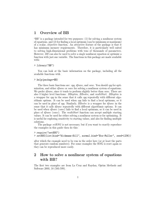
1Overview of BB“BB”is a package intended for two purposes:(1)for solving a nonlinear systemof equations,and(2)forfinding a local optimum(can be minimum or maximum)of a scalar,objective function.An attractive feature of the package is that ithas minimum memory requirements.Therefore,it is particularly well suitedto solving high-dimensional problems with tens of thousands of parameters. However,BB can also be used to solve a single nonlinear equation or optimize a function with just one variable.The functions in this package are made availablewith:>library("BB")You can look at the basic information on the package,including all the available functions wtih>help(package=BB)The three basic functions are:spg,dfsane,and sane.You should spg for opti-mization,and either dfsane or sane for solving a nonlinear system of equations.We prefer dfsane,since it tends to perform slightly better than sane.There arealso3higher level functions:BBoptim,BBsolve,and multiStart.BBoptim isa wrapper for spg in the sense that it calls spg repeatedly with different algo-rithmic options.It can be used when spg fails tofind a local optimum,or itcan be used in place of spg.Similarly,BBsolve is a wrapper for dfsane in thesense that it calls dfsane repeatedly with different algorithmic options.It canbe used when dfsane(sane)fails tofind a local optimum,or it can be used inplace of dfsane(sane).The multiStart function can accept multiple starting values.It can be used for either solving a nonlinear system or for optimizing.Itis useful for exploring sensitivity to starting values,and also forfinding multiple solutions.The package setRNG is not necessary,but if you want to exactly reproducethe examples in this guide then do this:>require("setRNG")>setRNG(list(kind="Wichmann-Hill",normal.kind="Box-Muller",seed=1236)) after which the example need to be run in the order here(or at least the partsthat generate random numbers).For some examples the RNG is reset again sothey can be reproduced more easily.2How to solve a nonlinear system of equations with BB?Thefirst two examples are from La Cruz and Raydan,Optim Methods and Software2003,18(583-599).1>expo3<-function(p){#From La Cruz and Raydan,Optim Methods and Software2003,18(583-599) n<-length(p)f<-rep(NA,n)onm1<-1:(n-1)f[onm1]<-onm1/10*(1-p[onm1]^2-exp(-p[onm1]^2))f[n]<-n/10*(1-exp(-p[n]^2))f}>p0<-runif(10)>ans<-dfsane(par=p0,fn=expo3)Iteration:0||F(x0)||:0.2024112iteration:10||F(xn)||=0.07536174iteration:20||F(xn)||=0.08777425iteration:30||F(xn)||=0.005029196iteration:40||F(xn)||=0.001517709iteration:50||F(xn)||=0.001769548iteration:60||F(xn)||=0.007896929iteration:70||F(xn)||=0.0001410588iteration:80||F(xn)||= 2.002796e-06>ans$par[1] 3.819663e-02 3.031250e-02 2.647897e-02 2.404688e-02 2.233208e-02 [6] 2.101498e-02 1.996221e-02 1.909301e-02 1.835779e-02-7.493381e-06 $residual[1]6.645152e-08$fn.reduction[1]0.6400804$feval[1]96$iter[1]85$convergence[1]0$message[1]"Successful convergence"Let us look at the output from dfsane.It is a list with7components.Themost important components to focus on are the two named“par”and“conver-2gence”.ans$par provides the solution from dfsane,but this is a root if andonly if ans$convergence is equal to0,i.e.ans$message should say“Successful convergence”.Otherwise,the algorithm has failed.Now,we show an example demonstrating the ability of BB to solve a largesystem of equations,N=10000.>trigexp<-function(x){n<-length(x)F<-rep(NA,n)F[1]<-3*x[1]^2+2*x[2]-5+sin(x[1]-x[2])*sin(x[1]+x[2])tn1<-2:(n-1)F[tn1]<--x[tn1-1]*exp(x[tn1-1]-x[tn1])+x[tn1]*(4+3*x[tn1]^2)+ 2*x[tn1+1]+sin(x[tn1]-x[tn1+1])*sin(x[tn1]+x[tn1+1])-8 F[n]<--x[n-1]*exp(x[n-1]-x[n])+4*x[n]-3F}>n<-10000>p0<-runif(n)>ans<-dfsane(par=p0,fn=trigexp,control=list(trace=FALSE))>ans$message[1]"Successful convergence">ans$resid[1]5.725351e-08The next example is from Freudenstein and Roth function(Broyden,Math-ematics of Computation1965,p.577-593).>froth<-function(p){f<-rep(NA,length(p))f[1]<--13+p[1]+(p[2]*(5-p[2])-2)*p[2]f[2]<--29+p[1]+(p[2]*(1+p[2])-14)*p[2]f}Now,we introduce the function BBsolve.For thefirst starting value,dfsaneused in the default manner does notfind the zero,but BBsolve,which triesmultiple control parameter settings,is able to successfullyfind the zero.>p0<-c(3,2)>dfsane(par=p0,fn=froth,control=list(trace=FALSE))$par[1]-9.822061-1.875381$residual3[1]11.63811$fn.reduction[1]25.58882$feval[1]137$iter[1]114$convergence[1]5$message[1]"Lack of improvement in objective function">BBsolve(par=p0,fn=froth)Successful convergence.$par[1]54$residual[1]3.659749e-10$fn.reduction[1]0.001827326$feval[1]100$iter[1]10$convergence[1]0$message[1]"Successful convergence"$cparmethod M NM2501Note that the functions dfsane,sane,and spg produce a warning message if convergence fails.These warnings have been suppressed in this vignette.4For the next starting value,BBsolvefinds the zero of the system,but dfsane (with defaults)fails.>p0<-c(1,1)>BBsolve(par=p0,fn=froth)Successful convergence.$par[1]54$residual[1]9.579439e-08$fn.reduction[1]6.998875$feval[1]1165$iter[1]247$convergence[1]0$message[1]"Successful convergence"$cparmethod M NM1501>dfsane(par=p0,fn=froth,control=list(trace=FALSE))$par[1]-9.674222-1.984882$residual[1]12.15994$fn.reduction[1]24.03431$feval[1]138$iter5[1]109$convergence[1]5$message[1]"Lack of improvement in objective function"Try random starting values.Run the following set of code many times.Thisshows that BBsolve is quite robust infinding the zero,whereas dfsane(withdefaults)is sensitive to starting values.Admittedly,these are poor startingvalues,but still it would be nice to have a strategy that has a high likelihood offinding a zero of the nonlinear system.>#two values generated independently from a poisson distribution with mean=10 >p0<-rpois(2,10)>BBsolve(par=p0,fn=froth)Successful convergence.$par[1]54$residual[1]7.330654e-08$fn.reduction[1]0.07273382$feval[1]91$iter[1]41$convergence[1]0$message[1]"Successful convergence"$cparmethod M NM2501>dfsane(par=p0,fn=froth,control=list(trace=FALSE))$par[1]546$residual[1]5.472171e-08$fn.reduction[1]490.618$feval[1]32$iter[1]31$convergence[1]0$message[1]"Successful convergence"2.1Finding multiple roots of a nonlinear system of equa-tionsNow,we introduce the function multiStart.This accepts a matrix of startingvalues,where each row is a single starting value.multiStart calls BBsolve foreach starting value.Here is a system of3non-linear equations,where eachequation is a high-degree polynomial.This system has12real-valued roots and126complex-valued roots.Here we will demonstrate how to identify all the12real roots using multiStart.Note that we specify the‘action’argument in thefollowing call to multiStart only to highlight that multiStart can be used forboth solving a system of equations and for optimization.The default is‘action=”solve”’,so it is really not needed in this call.>#Example>#A high-degree polynomial system(R.B.Kearfott,ACM1987)>#There are12real roots(and126complex roots to this system!)>#>hdp<-function(x){f<-rep(NA,length(x))f[1]<-5*x[1]^9-6*x[1]^5*x[2]^2+x[1]*x[2]^4+2*x[1]*x[3] f[2]<--2*x[1]^6*x[2]+2*x[1]^2*x[2]^3+2*x[2]*x[3]f[3]<-x[1]^2+x[2]^2-0.265625f}We generate100randomly generated starting values,each a vector of lengthequal to3.(Setting the seed is only necessary to reproduce the result shownhere.)7>setRNG(list(kind="Wichmann-Hill",normal.kind="Box-Muller",seed=123))>p0<-matrix(runif(300),100,3)#100starting values,each of length3 >ans<-multiStart(par=p0,fn=hdp,action="solve")>sum(ans$conv)#number of successful runs=99>pmat<-ans$par[ans$conv,]#selecting only converged solutions Now,we display the unique real solutions.>ans<-round(pmat,4)>ans[!duplicated(ans),][,1][,2][,3][1,]0.27990.4328-0.0142[2,]0.00000.51540.0000[3,]0.51540.0000-0.0124[4,]0.4670-0.21810.0000[5,]0.46700.21810.0000[6,]0.0000-0.51540.0000[7,]0.2799-0.4328-0.0142[8,]-0.46700.21810.0000[9,]-0.27990.4328-0.0142[10,]-0.51540.0000-0.0124[11,]-0.2799-0.4328-0.0142[12,]-0.4670-0.21810.0000We can also visualize these12solutions beautifully using a‘biplot’based onthefirst2principal components of the converged parameter matrix.>pc<-princomp(pmat)>biplot(pc)#you can see all12solutions beautifully like on a clock!8−0.3−0.2−0.10.00.1−0.3−0.2−0.10.00.1Comp.1C o m p .2123456789101112131415161718192021222324252627282930313233343536373839404142434445464748495051525354555657585960616263646566676869707172737475767778798081828384858687888990919293949596979899100−4−3−2−1012−4−3−2−1012Var 1Var 2Var 32.2Power polynomial method:Fleishman system of equa-tionsFleishman (Psychometrika 1978,p.521-532)developed an approach for simu-lating random numbers from non-normal distrinbutions,with specified valuesof skewness and kurtosis.This approach involves the solution of a system of polynomial equations.This system is also discussed in the paper by Demirtas and Hedeker (Communications in Statistics 2008,p.1682-1695;Equations on p.1684)and is given as follows:>fleishman <-function(x,r1,r2){b <-x[1]c <-x[2]d <-x[3]f <-rep(NA,3)f[1]<-b^2+6*b *d +2*c^2+15*d^2-1f[2]<-2*c *(b^2+24*b*d +105*d^2+2)-r1f[3]<-b*d +c^2*(1+b^2+28*b *d)+d^2*(12+48*b*d +141*c^2+225*d^2)-r2/24f }9We only use3equations,since1st equation is trivially solved by a=-c.Here we describe an experiment based on Fleishman(Psychometrika1978,p.521-532),and is reproduced as follows.We randomly picked10scenarios(more or less randomly)from Table1of Fleishman(1978):>rmat<-matrix(NA,10,2)>rmat[1,]<-c(1.75,3.75)>rmat[2,]<-c(1.25,2.00)>rmat[3,]<-c(1.00,1.75)>rmat[4,]<-c(1.00,0.50)>rmat[5,]<-c(0.75,0.25)>rmat[6,]<-c(0.50,3.00)>rmat[7,]<-c(0.50,-0.50)>rmat[8,]<-c(0.25,-1.00)>rmat[9,]<-c(0.0,-0.75)>rmat[10,]<-c(-0.25,3.75)We solve the system of equations for the above10specifications of skewnessand kurtosis3times,each time with a different random starting seed.>#1>setRNG(list(kind="Mersenne-Twister",normal.kind="Inversion",seed=13579)) >ans1<-matrix(NA,nrow(rmat),3)>for(i in1:nrow(rmat)){x0<-rnorm(3)#random starting valuetemp<-BBsolve(par=x0,fn=fleishman,r1=rmat[i,1],r2=rmat[i,2])if(temp$conv==0)ans1[i,]<-temp$par}Successful convergence.Successful convergence.Successful convergence.Successful convergence.Successful convergence.Successful convergence.Successful convergence.Successful convergence.Successful convergence.Successful convergence.>ans1<-cbind(rmat,ans1)>colnames(ans1)<-c("skew","kurtosis","B","C","D")>ans1skew kurtosis B C D[1,] 1.75 3.75-0.9296606 3.994967e-010.036466986[2,] 1.25 2.00-0.9664061 2.230888e-010.00586254310[3,] 1.00 1.750.9274664 1.543072e-010.015885481[4,] 1.000.50 1.1146549 2.585245e-01-0.066013188[5,]0.750.25-1.2977959 2.727191e-010.150766137[6,]0.50 3.00-0.7933810 5.859729e-02-0.063637596[7,]0.50-0.50-1.3482151 1.886967e-010.153679396[8,]0.25-1.00-1.36289609.474017e-020.146337538[9,]0.00-0.75 1.1336220-6.936031e-13-0.046731705[10,]-0.25 3.75 1.5483100-6.610187e-02-0.263217996>#2>setRNG(list(kind="Mersenne-Twister",normal.kind="Inversion",seed=91357)) >ans2<-matrix(NA,nrow(rmat),3)>for(i in1:nrow(rmat)){x0<-rnorm(3)#random starting valuetemp<-BBsolve(par=x0,fn=fleishman,r1=rmat[i,1],r2=rmat[i,2])if(temp$conv==0)ans2[i,]<-temp$par}Successful convergence.Successful convergence.Successful convergence.Successful convergence.Successful convergence.Successful convergence.Successful convergence.Successful convergence.Successful convergence.Successful convergence.>ans2<-cbind(rmat,ans2)>colnames(ans2)<-c("skew","kurtosis","B","C","D")>ans2skew kurtosis B C D[1,] 1.75 3.75-0.9296606 3.994967e-010.03646699[2,] 1.25 2.000.9664061 2.230888e-01-0.00586255[3,] 1.00 1.75-0.9274663 1.543073e-01-0.01588548[4,] 1.000.50-1.1146552 2.585249e-010.06601337[5,]0.750.25-1.2977961 2.727192e-010.15076629[6,]0.50 3.000.7933810 5.859729e-020.06363759[7,]0.50-0.50-1.3482151 1.886967e-010.15367938[8,]0.25-1.00 1.36289639.474021e-02-0.14633771[9,]0.00-0.75 1.1336221-2.520587e-13-0.04673174[10,]-0.25 3.750.7503153-2.734120e-020.07699283>#3>setRNG(list(kind="Mersenne-Twister",normal.kind="Inversion",seed=79135))11>ans3<-matrix(NA,nrow(rmat),3)>for(i in1:nrow(rmat)){x0<-rnorm(3)#random starting valuetemp<-BBsolve(par=x0,fn=fleishman,r1=rmat[i,1],r2=rmat[i,2]) if(temp$conv==0)ans3[i,]<-temp$par}Successful convergence.Successful convergence.Successful convergence.Successful convergence.Successful convergence.Successful convergence.Successful convergence.Successful convergence.Successful convergence.Successful convergence.>ans3<-cbind(rmat,ans3)>colnames(ans3)<-c("skew","kurtosis","B","C","D")>ans3skew kurtosis B C D[1,] 1.75 3.750.9207619 4.868014e-01-0.07251973[2,] 1.25 2.00 1.1312711 4.094915e-01-0.12535043[3,] 1.00 1.750.9274666 1.543073e-010.01588543[4,] 1.000.50-1.1146554 2.585250e-010.06601345[5,]0.750.25 1.0591737 1.506888e-01-0.02819626[6,]0.50 3.00-0.7933811 5.859729e-02-0.06363759[7,]0.50-0.50 1.1478497 1.201563e-01-0.05750376[8,]0.25-1.00-1.36289599.474013e-020.14633745[9,]0.00-0.75-1.1336219-1.156859e-160.04673169[10,]-0.25 3.75 1.5483099-6.610187e-02-0.26321798>This usuallyfinds an accurate root of the Fleishman system successfully inall50cases(but may occassionaly fail with different seeds).An interesting aspect of this exercise is the existence of multiple roots to the Fleishman system.There are4valid roots for any”feasible”combina-tion of skewness and kurtosis.These4roots can be denoted as:(b1,c1,−d1), (−b1,c1,d1),(b2,c2,−d2),(−b2,c2,d2),where b1,c1,d1,b2,c2,d2are all positive (except for the coefficient c which is zero when skewness is zero).Fleishman only reports thefirst root,whereas we can locate the other roots using BBsolve.The experiments demonstrate quite convincingly that the wrapper function BBsolve can successfully solve the system of equations associated with the power polynomial method of Fleishman.123How to optimize a nonlinear objective func-tion with BB?The basic function for optimization is spg.It can solve smooth,nonlinear op-timization problems with box-constraints,and also other types of constraintsusing projection.We would like to direct the user to the help page for manyexamples of how to use spg.Here we discuss an example involving estimation ofparameters maximizing a log-likelihood function for a binary Poisson mixturedistribution.>poissmix.loglik<-function(p,y){#Log-likelihood for a binary Poisson mixture distributioni<-0:(length(y)-1)loglik<-y*log(p[1]*exp(-p[2])*p[2]^i/exp(lgamma(i+1))+(1-p[1])*exp(-p[3])*p[3]^i/exp(lgamma(i+1)))return(sum(loglik))}>#Data from Hasselblad(JASA1969)>poissmix.dat<-data.frame(death=0:9,freq=c(162,267,271,185,111,61,27,8,3,1))There are3model parameters,which have restricted domains.So,we definethese constraints as follows:>lo<-c(0,0,0)#lower limits for parameters>hi<-c(1,Inf,Inf)#upper limits for parametersNow,we maximize the log-likelihood function using both spg and BBoptim,with a randomly generated starting value for the3parameters:>p0<-runif(3,c(0.2,1,1),c(0.8,5,8))#a randomly generated vector of length3 >y<-c(162,267,271,185,111,61,27,8,3,1)>ans1<-spg(par=p0,fn=poissmix.loglik,y=y,lower=lo,upper=hi,control=list(maximize=TRUE,trace=FALSE))>ans1$par[1]0.6400942.6634301.256131$value[1]-1989.946$gradient[1]0.0001523404$fn.reduction[1]-209.040513$iter[1]42$feval[1]44$convergence[1]0$message[1]"Successful convergence">ans2<-BBoptim(par=p0,fn=poissmix.loglik,y=y,lower=lo,upper=hi,control=list(maximize=TRUE)) iter:0f-value:-2198.986pgrad:360.6254iter:10f-value:-1991.173pgrad: 3.212342iter:20f-value:-1990.47pgrad: 1.571746iter:30f-value:-1990.053pgrad:0.6429582iter:40f-value:-1989.946pgrad:0.3574752iter:50f-value:-1989.946pgrad:0.01283524iter:60f-value:-1989.946pgrad:0.0009822543 Successful convergence.>ans2$par[1]0.64012482.66339091.2560779$value[1]-1989.946$gradient[1]0.0001591616$fn.reduction[1]-209.0405$iter[1]65$feval[1]169$convergence[1]014$message[1]"Successful convergence"$cparmethod M250Note that we had to specify the‘maximize’option inside the control list to let the algorithm know that we are maximizing the objective function,since the default is to minimize the objective function.Also note how we pass the data vector‘y’to the log-likelihood function,possmix.loglik.Now,we illustrate how to compute the Hessian of the log-likelihood at the MLE,and then how to use the Hessian to compute the standard errors for the parameters.To compute the Hessian we require the package”numDeriv.”>require(numDeriv)>hess<-hessian(x=ans2$par,func=poissmix.loglik,y=y)>#Note that we have to supplied data vector`y'>hess[,1][,2][,3][1,]-907.1186-341.25895-270.22619[2,]-341.2590-192.78641-61.68141[3,]-270.2262-61.68141-113.47653>se<-sqrt(diag(solve(-hess)))>se[1]0.19467970.25047060.3500305Now,we explore the use of multiple starting values to see if we can iden-tify multiple local maxima.We have to make sure that we specify‘action=”optimize”’,because the default option in multiStart is”solve”.>#3randomly generated starting values>p0<-matrix(runif(30,c(0.2,1,1),c(0.8,8,8)),10,3,byrow=TRUE) >ans<-multiStart(par=p0,fn=poissmix.loglik,action="optimize", y=y,lower=lo,upper=hi,control=list(maximize=TRUE)) Parameter set:1...iter:0f-value:-2629.616pgrad: 5.149479iter:10f-value:-2001.398pgrad:0.01419494Successful convergence.Parameter set:2...iter:0f-value:-2046.752pgrad:172.2726iter:10f-value:-1990.065pgrad:0.891859615iter:20f-value:-1990.031pgrad: 4.181468 iter:30f-value:-1990.291pgrad:8.707709 Successful convergence.Parameter set:3...iter:0f-value:-2722.155pgrad:7.534183 iter:10f-value:-1991.544pgrad: 3.31378 iter:20f-value:-1990.761pgrad:8.096627 iter:30f-value:-1989.949pgrad:0.5093102 iter:40f-value:-1989.946pgrad:0.0177306 Successful convergence.Parameter set:4...iter:0f-value:-3692.509pgrad: 6.213669 iter:10f-value:-1990.145pgrad: 2.718772 iter:20f-value:-1990.188pgrad:7.280146 iter:30f-value:-1989.946pgrad:0.0004024514 Successful convergence.Parameter set:5...iter:0f-value:-2996.35pgrad:7.452469iter:10f-value:-1997.898pgrad: 2.430247 iter:20f-value:-1989.959pgrad:0.3875152 iter:30f-value:-1989.949pgrad:0.5795755 iter:40f-value:-1989.946pgrad:0.01441776 Successful convergence.Parameter set:6...iter:0f-value:-4492.74pgrad: 6.965384iter:10f-value:-2001.472pgrad:8.750483 Successful convergence.Parameter set:7...iter:0f-value:-3357.482pgrad: 6.954945 iter:10f-value:-1991.658pgrad: 2.799363 iter:20f-value:-1989.997pgrad:0.6908181 iter:30f-value:-1989.959pgrad: 1.203134 iter:40f-value:-1989.946pgrad:0.001996341 iter:50f-value:-1989.946pgrad:0.001468834 Successful convergence.Parameter set:8...iter:0f-value:-3172.301pgrad: 5.470799 iter:10f-value:-2007.457pgrad: 2.315072 Successful convergence.Parameter set:9...iter:0f-value:-4019.753pgrad: 6.606661 iter:10f-value:-1993.303pgrad:32.41122 iter:20f-value:-1990.292pgrad: 2.832038 iter:30f-value:-1989.956pgrad: 1.914161 iter:40f-value:-1989.946pgrad:0.02872412 Successful convergence.16Parameter set:10...iter:0f-value:-2045.64pgrad: 3.808228iter:10f-value:-1991.291pgrad: 2.49011iter:20f-value:-1990.413pgrad: 1.413719iter:30f-value:-1989.946pgrad:0.03627974iter:40f-value:-1989.946pgrad:0.01119133iter:50f-value:-1989.946pgrad:0.0002614797Successful convergence.>#selecting only converged solutions>pmat<-round(cbind(ans$fvalue[ans$conv],ans$par[ans$conv,]),4)>dimnames(pmat)<-list(NULL,c("fvalue","parameter1","parameter2","parameter3")) >pmat[!duplicated(pmat),]fvalue parameter1parameter2parameter3[1,]-1996.6890.3095 2.6448 1.9311[2,]-1989.9460.3599 1.2561 2.6634[3,]-1989.9460.6401 2.6634 1.2561[4,]-1995.5720.4053 2.6018 1.8435[5,]-1997.2050.7042 1.9525 2.6274>Here multiStart is able to identifies many solutions.Two of these,the2nd and3rd rows,appear to be global maxima with different parameter values.Actually,there is only one global maximum.It is due to the‘label switching’problem thatwe see2solutions.The multiStart algorithm also identifies three local maximawith inferior values.17。
广州大学硕士生导师一览表

广州大学硕士生导师一览表(按专业)陈文立目录人物简介科研情况编辑本段人物简介陈文立,男,1940年出生。
大学本科学历。
重庆师范学院数学系教授。
中国、美国数学会会员,《数学评论》评论员,曾入选美国《世界名人录(12版)》。
[1]编辑本段科研情况专业特长与业绩:数论(初等数论、解析数论)、组合论(组合计数、拉姆塞理论)及数学教育(高等数学指导中学数学、数学继续教育、数学方法论)。
自然数乘法分拆数的上界,期刊名称:数学学报,32:5,1989,第一作者。
关于北法分拆数的上界,期刊名称:科学通报:37:11,1992,第一作者。
科学性、直观性、前瞻性一改革《高等几何》课程的几点建议,期刊名称:数学教育学报,7:1,1998,第一作者。
关于第二类Stirling数的某些模性质,•会议名称:国际组合数学学术会议(论文集),第一作者。
数学归纳法,四川科学技术出版社,1987,专著,第一作者。
参数方程,重庆出版社,1987,专著,第二作者。
其它在有关学术论文计五十余篇。
在《数学评论》上发表有影响的评论文章四十多篇。
曾获1989年市先进个人、校优秀教学成果奖、省、市优秀论文奖等奖励。
[1]单墫单墫教授1943年11月1日生于天津,江苏扬州市人,南京师范大学数学与计算机科学学院教授、博士生导师、广州大学教育软件所兼职研究员,享受政府特殊津贴。
1964年毕业于扬州师范学院数学系后在南京人民中学任教,1978年考入中国科学技术大学,师从著名数学家王元院士攻读研究生,1983年在中国科学技术大学获理学博士学位,毕业后,留在中国科学技术大学校任教。
1989年起,任教于南京师范大学,曾任南京师范大学数学系主任、南京师范大学学术委员会委员、学位评定委员会委员、中共南京师范大学委员会委员、南京市第九届政协委员。
[1]单墫教授在数学领域的初等数论、解析数论和组合数学研究方面取得了一些国际先进水平的成果,发表了30多篇具有较高水平的学术研究论文。
ExcelSolver的用法

Excel Solver的用法电脑相关 2009-06-26, 22:13Solver是Excel一个功能非常强大的插件(Add-Ins),可用于工程上、经济学及其它一些学科中各种问题的优化求解,使用起来非常方便,Solver包括(但不限于)以下一些功能:1、线性规划2、非线性规划3、线性回归,多元线性回归可以用Origin求解,也可以用Excel的linest函数或分析工具求解。
4、非线性回归5、求函数在某区间内的极值注意:Solver插件可以用于解决上面这些问题,并不是说上面这些问题Solver 一定可以解决,而且有时候Solver给出的结果也不一定是最优的。
Solver安装方法:Solver是Excel自带的插件,不需要单独下载安装。
但Excel默认是不启用Solver的,启用方法:在"工具"菜单中点击“插件”,在Solver Add-In前面的方框中打勾,然后点OK,Excel会自动加载Solver,一旦启用成功,以后Sovler 就会在"工具"菜单中显示。
Solver求解非线性回归问题的方法:假设X和Y满足这样一个关系:Y=L(1-10-KX),实验测得一组X和Y的值如下:X Y0 00.54 1830.85 2251.50 2862.46 3803.56 4705.00 544求L和K的值。
在Excel中随便假设一组L和K的值,比如都假设为1,以这组假设的值,求出一组Y’,然后再求出一组(X-Y)2的值,再将求出的这组(X-Y)2的值用Sum函数全部加起来(下面的图中,全部加起来结果在$G$22这个单元格中)。
然后点击“工具”菜单中的Solver,将Set Target Cell设为$G$22这个单元格,将By Changing Cells设为$F$8:$F9这两个单元格,即改变L和K的值,Equal To选中Min这项,其他的选项不用理会,如下图:然后点右上角的Solver,$F$8:$F9就会改变,改变之后的值即为优化的L和K 值。
DearEditor,DearR...
Dear Editor, Dear Reviewer,I deeply appreciate the time and effort you’ve spent on reviewing my manuscript. Your comments are really thoughtful and in-depth and I do honestly agree with most of them. Before I address the comments individually, please allow me to explain several difficulties I encountered, which eventually resulted in the limitations of the manuscript, which were also pointed out in your comments.The primary purpose of writing this manuscript is to borrow the data assimilation framework for understanding the impact of the uncertainties in the physical models and their parameters, which has been actively developed and successfully applied in other disciplines, into the seismic modeling and inversion community. This adoption process is not trivial and to make it tractable and also more readable I made simplifications, which lead to limitations of the derived formulation. In addition to the Gaussian assumptions for the stochastic noise processes, which will be addressed in detail later, I also simplified the form of the wave equation, which does not include rotation of the Earth, self-gravitation and other important effects such as poroelasticity. The stochastic noise processes in the dynamic model and its boundary and initial conditions are treated as additive, which might not be suitable for all situations. In the revised manuscript, I pointed out the limitations of my formulation more clearly both in the introduction section and also through out the text.I think the justification for introducing stochastic noises into the wave equation and its initial and boundary conditions is two-folded. First, our deterministic model is not perfect and it is difficult, if possible at all, to fully eliminate all its deficiencies. Second, the impact of the uncertainties in the dynamic model, in particular, the impact on the estimation of model parameters, needs to be evaluated, especially when the procedures of seismological inversions are becoming more and more precise under the full-wave framework. This manuscript is an attempt to address some of the issues under the full-wave framework. Its scope and depth are inherently limited by my own background and capability. But I do hope that it could become useful at some point during the development and application of the full-wave methodology.Responses to major remarks and questions:1.The Gaussian assumption for the stochastic noise processes indeed brings muchconvenience into the derivation. And a direct benefit in terms of readability is that the resulting equations have similarities with classical formulations based on least-squares. The quadratic-form misfit functional and quadratic-form model regularization, which are often employed in classical formulations, correspond to Gaussian likelihood and Gaussian priors used in this manuscript. The Bayesian framework itself is not limited to Gaussian statistics. An example of using exponential and truncated exponential distributions with the Bayesian framework and a grid-search optimization algorithm for centroid moment tensor inversions is given in a separate manuscript, “Rapid Centroid Moment Tensor (CMT) Inversion in a Three-Dimensional Earth Structure Model for Earthquakes inSouthern California (Lee, Chen & Jordan, GJI)”, which is currently under review.For probability densities that are non-Gaussian, the formulation still has applicability if a Gaussian distribution provides a sufficiently good approximation to the actual distribution from a practical point of view. An optimal Gaussian approximation can be found from the first and second moments of the actual distribution. For nonlinear systems such as the one used in solving seismological inverse problems, the system is linearized around the current mean and the covariance is propagated using the linearized dynamics. For limited propagation ranges, a Gaussian distribution could indeed provide a sufficiently good approximation locally. When nonlinearities are high and uncertainties need to be evolved over long ranges, the Gaussian assumption may no longer be valid. A promising new development to account for non-Gaussian probabilities is the generalized polynomial chaos (gPC) theory, which uses a polynomial based stochastic space to represent and propagate uncertainties. The completeness of the space warrants accurate representations of any probability densities and certain bases can be selected to represent particular types of probability densities with the fewest number of terms. In gPC, a perfect Gaussian distribution can be represented using 2 Hermite polynomials and a uniform distribution can be represented using 2 Legendre polynomials. Polynomial math can therefore be employed to make the interactions among various probability densities tractable and the results can be calculated in the polynomial space, which has favorable properties in terms of continuity and differentiability. I am still working on the formulation based on the gPC theory. If successful, it will be documented in a future publication. In the introduction section of the revised manuscript, I’ve added a paragraph to indicate the limitations and applicability of the Gaussian assumption.2.The origins of the uncertainties are sometimes difficult to classify and explain andbecause of such unknown and/or unexplained origins, we often work toward reducing them to stochastic processes and try to quantify their statistical properties using direct and/or indirect methods. I adopted the Bayesian framework in this study, which is essentially a subjective interpretation of probability. Some types of uncertainties depend on chance (i.e. aleatory or statistical) and others are due to the lack of knowledge (i.e. epistemic or systematic). It is difficult to separate different types of uncertainties in the derivation, therefore individual stochastic noises introduced in the derivation do not correspond to a particular type of uncertainty and the noises in the wave equation and its boundary/initial conditions could have both aleatory and epistemic origins. Some common origins of uncertainties, in addition to the uncertainties in the model parameters, include but are not limited to, the errors in the mathematical model, the numerical method used for solving the mathematical model, and errors in the initial and boundary conditions. For epistemic uncertainties, efforts need to be made to better understand the system and sometimes model errors can be evaluated by using improved observations. But in general, to evaluate epistemic uncertainties requires more effort and usually involves discovering new physics or mechanisms, which could be nonlinear. Treating those stochastic noises as additive is certainly a limitation of my formulation and I pointed that out in therevised manuscript. And I also included more explanations about possible origins of the uncertainties that I am aware of in the revised manuscript. But the primary purpose of introducing those stochastic noise processes is to account for uncertainties due to unknown/unexplained origins. The recent development of Dempster-Shafer theory provides a systematic framework for representing epistemic plausibility and has been used in machine learning. A short essay about this new development can be found at /assets/downloads/articles/article48.pdf, but to adopt it in this study is too involved and might not be necessary at the current development stage of full-wave seismological inversions. In terms of nomenclature, I realized that “model error” might be misleading and I changed that to “model residual” in the revised manuscript.3.Possible reasons that could cause deviations from the traction-free boundarycondition might include lithosphere-atmosphere coupling, deviation from the continuum model for materials in the near-surface environment, numerical errors caused by, for instance, errors in the numerical representation of the actual topography, etc. The Earth is constantly in motion. The quiescent-past initial condition for one seismic event could be violated in practice if we consider motions caused by, for instance, other seismic events, the Earth’s ambient noise field and the constant hum of the Earth caused by atmosphere-ocean-seafloor coupling. I’ve added those possible explanations and some references into the revised manuscript. These are some possible causes that I am aware of. It is certainly not complete. There might be also unknown mechanisms or noises that can cause deviations from the theoretical initial and boundary conditions.4.It is true that the errors in the elastic parameters are not independent. I’veremoved the sentence from the revised manuscript. In practice, we only need to introduce 21 independent distributions. To account for equality constraints among elastic parameters, the delta distribution can be introduced to represent the corresponding conditional probabilities. A delta distribution can be treated as the limit of a Gaussian distribution with its variance approaching zero. Going through the same steps in the derivation, the equations for updating the elastic parameters will then include a number of equations that repeat the symmetry conditions among all elastic parameters. I’ve added several sentences in the revised manuscript to clarify this point. It is also true that the Gaussian distribution is only an approximation to the actual distribution, since the elastic parameters need to satisfy stability requirements. The Gaussian approximation is only valid locally when the current mean (i.e. the reference elastic tensor for the current iteration) satisfy the stability requirements and the variance is not too large. I added several sentences in the revised manuscript to clarify this point. Some of the positivity constraints can be removed through a change of variable, but I did not explore in that direction. The quadratic model regularization term that is often used in the objective functions in the classical formulations also imply a Gaussian distribution for structural parameters. But I do fully agree that one should not adopt Gaussian distributions for elastic parameters too easily just for mathematical convenience.Responses to minor remarks and questions:1.I do realize that using the term “full-physics” actually contradicts with theprimary goal of the formulation, which is actually to account for inadequacies in the physical model. On the other hand, I am also concerned that the use of “full waveform” might cause the misunderstanding that I am inverting the completed seismograms from first arrival to coda point by point. I replaced “full-physics” in the title and throughout the text with the term “full-wave”. I hope that is an acceptable term.2.I have re-worded this sentence and added the two references of Bamberger et al.,provided by the reviewer. Many thanks for correcting me on this.3.I do agree that adding the source index indeed complicates the formulation evenfurther. However it might make the discussion on computational costs and the distinctions between scattering-integral and adjoint formulations more clear. I agree that at this point I did sacrifice readability for some degree of clarity. I do apologize for the inconvenience caused by this notation.4.I thank the reviewer for raising this issue. Yes, I did consider this notation.However I was concerned that readers who are not familiar with the methodology might mistaken it as the global optimal. I used the iteration index γ in the iterative Euler-Lagrange equations to indicate the optimal models for each iteration. I hope this is acceptable.5.The statement on source inversion is indeed over simplified. I was trying tomotivate the discussion on separating phase and amplitude information in the complete waveforms. I’ve re-worded the sentence and added a paragraph in section 4.2 to discuss finite-source inversion results from Fichtner & Tkalčić in the revised manuscript.6.I fully acknowledge the importance of the Born approximation in tomography. Ihave re-worded the sentence in the revised manuscript to avoid misleading the readers. The limitation of the Born approximation that I am referring to only applies to direct waveform inversions using waveform differences as data functionals. I’ve re-worded some sentences to emphasize this point. The Born approximation can be used for obtaining the exact sensitivity kernels of other types of data functionals such as cross-correlation travel-time. It actually plays a fundamental role in seismic tomography.7.Yes, it should be correlogram. Many thanks for correcting this mistake in mymanuscript.8.Yes, I agree that the example that I used is not full-physics. I changed “full-physics” to “full-wave” and re-worded a few sentences in the paragraph to emphasize that.9.I’ve added the reference for Fichtner et al. (2010b) and a more extended discussabout the improvements both in resolution and in resolving anisotropy.10.I fully agree. The number of simulation counts used in this manuscript is just togive a general guideline for estimating computational costs. The design of line search is flexible and can change the number of simulations. I added a sentence in the revised manuscript to emphasize that.11.Yes, I have added a few sentences to clarify that this method only works for non-dissipative media. The PML absorbing boundary conditions need to be handledwith care. One possibility that seems to work is to store the wave-field going through the absorbing boundaries and play it back during the simulation with the negative time step. But in this case, additional storage as well as IO costs, which could be substantial depending on the size of the mesh, is needed.12.I have corrected and updated the references. Many thanks for checking andpointing out the errors. I really appreciate it.I hope the responses above address your comments and answer your questions satisfactorily. Thanks very much for your review and I truly appreciate your comments. Best regards,Po Chen。
A New Approach for Filtering Nonlinear Systems
computational overhead as the number of calculations demanded for the generation of the Jacobian and the predictions of state estimate and covariance are large. In this paper we describe a new approach to generalising the Kalman filter to systems with nonlinear state transition and observation models. In Section 2 we describe the basic filtering problem and the notation used in this paper. In Section 3 we describe the new filter. The fourth section presents a summary of the theoretical analysis of the performance of the new filter against that of the EKF. In Section 5 we demonstrate the new filter in a highly nonlinear application and we conclude with a discussion of the implications of this new filter1
Tቤተ መጻሕፍቲ ባይዱ
= = =
δij Q(i), δij R(i), 0, ∀i, j.
(3) (4) (5)
Adaptive tracking control of uncertain MIMO nonlinear systems with input constraints

article
info
abstract
In this paper, adaptive tracking control is proposed for a class of uncertain multi-input and multi-output nonlinear systems with non-symmetric input constraints. The auxiliary design system is introduced to analyze the effect of input constraints, and its states are used to adaptive tracking control design. The spectral radius of the control coefficient matrix is used to relax the nonsingular assumption of the control coefficient matrix. Subsequently, the constrained adaptive control is presented, where command filters are adopted to implement the emulate of actuator physical constraints on the control law and virtual control laws and avoid the tedious analytic computations of time derivatives of virtual control laws in the backstepping procedure. Under the proposed control techniques, the closed-loop semi-global uniformly ultimate bounded stability is achieved via Lyapunov synthesis. Finally, simulation studies are presented to illustrate the effectiveness of the proposed adaptive tracking control. © 2011 Elsevier Ltd. All rights reserved.
高维半线性耗散波动方程外问题解的整体存在性
高维半线性耗散波动方程外问题解的整体存在性
解:
由于高维半线性耗散波动方程涉及到多个变量和不同的空间维度,因此它的外问题解的整体存在性取决于整个方程的情况。
一般来说,只有在下列条件满足时,该问题的解的存在性才能得到保证:
1. 方程必须具有足够的正则性,即可以由具有确定的初值的C1类正则解决。
2. 对邻域的解的正则性要求:方程的解的收敛必须满足Lipschiz条件,即在每一个时刻t,解的导数必须是连续的。
3. 必须满足一定的初值条件:在时间t=0处给定一个稳定的初值。
4. 提供正确的耗散项,使得方程具有稳定性,即该系统必须有能力收敛到解的本源状态(t→∞)。
如果上述条件均满足,高维半线性耗散波动方程的外问题解将是存在的,并且解的存在性是独立于初始条件的,即它可以由不同的初始条件产生不同的解。
非线性函数中英文对照外文翻译文献

中英文对照翻译(文档含英文原文和中文翻译)一个新的辅助函数的构造方法的全局优化非线性函数优化问题中具有许多局部极小,在他们的搜索空间中的应用,如工程设计,分子生物学是广泛的,和神经网络训练.虽然现有的传统的方法,如最速下降方法,牛顿法,拟牛顿方法,信赖域方法,共轭梯度法,收敛迅速,可以找到解决方案,为高精度的连续可微函数,这在很大程度上依赖于初始点和最终的全局解的质量很难保证.在全局优化中存在的困难阻碍了许多学科的进一步发展.因此,全局优化通常成为一个具有挑战性的计算任务的研究.一般来说,设计一个全局优化算法是由两个原因造成的困难:一是如何确定所得到的最小是全球性的(当时全球最小的是事先不知道),和其他的是,如何从中获得一个更好的最小跳.对第一个问题,一个停止规则称为贝叶斯终止条件已被报道.许多最近提出的算法的目标是在处理第二个问题.一般来说,这些方法可以被类fi主要分两大类,即:(一)确定的方法,及(ii)的随机方法.随机的方法是基于生物或统计物理学,它跳到当地的最低使用基于概率的方法.这些方法包括遗传算法(GA),模拟退火法(SA)和粒子群优化算法(PSO).虽然这些方法有其用途,它们往往收敛速度慢和寻找更高精度的解决方案是耗费时间.他们更容易实现和解决组合优化问题.然而,确定性方法如填充函数法,盾构法,等,收敛迅速,具有较高的精度,通常可以找到一个解决方案.这些方法往往依赖于修改目标函数的函数“少”或“低”局部极小,比原来的目标函数,并设计算法来减少该fiED功能逃离局部极小更好的发现.引用确定性算法中,扩散方程法,有效能量的方法,和积分变换方法近似的原始目标函数的粗结构由一组平滑函数的极小的“少”.这些方法通过修改目标函数的原始目标函数的积分.这样的集成是实现太贵,和辅助功能的最终解决必须追溯到原始目标函数的最小值,而所追踪的结果可能不是真正的全球最小的问题.终端器无约束子能量法和动态隧道方法修改fiES的目标函数的基础上的动态系统的稳定性理论的全局优化的梯度下降算法的杂交方法.这些方法都将动态系统和相应的计算非常耗时,尤其是目标函数的维数的增加,因为他们的好点是通过搜索沿各坐标到终止的发现.拉伸函数方法是一个辅助函数法,利用以前的搜索得到的信息使目标函数和帮助算法跳出局部最小更有效.这种技术已被纳入PSO的提高找到全局极小的成功率.然而,这种混合算法是建立在一个随机的方法,其收敛速度慢、应用更易与低维问题.填充函数法是另一个辅助函数法作案fiES为目标函数的填充函数,然后找到更好的局部极小值逐步优化填充函数构造上得到的最小值.填充函数法为我们提供了一个好主意,使用局部优化技术来解决全局优化问题.如果无法估计的参数可以得到解决,设计的填充函数可以应用于高维函数,填充函数方法在文献中的前途是光明的.掘进方法修改fiES的目标函数,以确保未来的出发点具有相同的函数值所得到的最小离获得一个,从而找到全局极小的概率增加.一个连续的会话的方法(SCM)将目标函数转化为一个在函数值都高于得到的地区没有局部极小或固定点,除了预fi固定值.这个方法似乎有希望如果通过预fi造成不影响固定的点被排除在外..不管拉伸功能的方法,已设计的填充函数法,或隧道算法的使用,他们往往依赖于几个关键的参数是不同的fi邪教的预估中的应用,如在极小的存在和上下的目标函数的导数边界的间隔长度.因此,一个在理论上有效的辅助函数法是困难的fi邪教在实践中,由于参数的不确定性,实现.一一维函数的一个例子如下:25604712)(234+-+-=x x x x x f显然,1和2说明了“墨西哥帽”效应出现在辅助函数法(已填充函数法和拉伸函数法)在一个地方点x ∗= 4.60095.不必要的影响,即引入新的局部极小值,通过参数设置不当等引起的.新推出的局部极小值将增加原问题的复杂性和影响算法的全局搜索.因此,一个有效的参数调节方便的辅助功能的方法是值得研究的.基于此,在本文中,我们给出了一个简单的两阶段的函数变换方法,转换1398纽约王骥,J. S.张/数学和计算机和数学建模 47(2008)1396–1410.x *= 4.60095的功能定义(3).“墨西哥帽”效应出现在两个点原目标函数)(x f 迅速下降的收敛性和高的能力逐渐找到更好的解决方案,在更广阔的区域的一个辅助功能.这个想法是,填充函数法很相似.具体来说,我们首先发现的原始目标函数的局部最小.然后拉伸函数法和模拟填充函数法对目标函数进行连续的两个阶段的转换.构建的功能是在原来的目标函数值是高于获得一个在第一步区下降,而一个固定点必须在更好的区域存在.接下来,我们尽量减少辅助功能找到它的一个固定点(一个好点的)(x f 比局部极小获得之前),然后下一个局部优化的出发点.我们重复这个过程直到终止.在新方法中,参数容易设置,例如两个常数可以被预处理,由于辅助函数的性质是不依靠不同的参数来实现,虽然两个参数中引入辅助函数.上一集的尺寸为50,与其他方法的比较表明,新的算法是更有效的标准测试问题的数值试验.A new constructing auxiliary function method for globaloptimizationNonlinear function optimization problems which possess many local minimizers in their search spaces are widespread in applications such as engineering design, molecular biology, and neural network training. Although the existing traditional methods such as the steepest descentmethod, Newton method, quasi Newton methods, trust region method, and conjugate gradient method converge rapidly and can find the solutions with high precision for continuously differentiable functions, they rely heavily on the initial point and the quality of the final global solution is hard to guarantee. The existing difficulty in global optimization prevents many subjects from developing further.Therefore, global optimization generally becomes a challenging computational task for researchers.Generally speaking, the difficulty in designing an algorithm on global optimization is due to two reasons: One is how to determine that the obtained minimum is a global one (when the global minimum is not known in advance), and the other is that how to jump from the obtained minimum to a better one. In treating the first problem, a stopping rule named the Bayes in termination condition has been reported.Many recently proposed algorithms aim at dealing with the second problem. Generally, these methods can be classfied into two main categories, namely: (i)deterministic methods, and (ii) stochastic methods. The stochastic methods are based on biology or statistical physics,which jump to the local minimum by using a probability based approach. These methods include genetic algorithm(GA), simulated annealing method (SA) and particle swarm optimization method (PSO). Although these methods have their uses, they often converge slowly and finding a solution with higher precision is time consuming.They are easier to implement and to solve combinational optimization problems. However, deterministic methods such as the filled function method, tunneling method, etc, converge more rapidly, and can often find a solution with a higher precision. These methods often rely on modifying the objective function to a function with “fewer” or “lower” local minimizers than the original objective function, and then design algorithms to minimize the modified function to escape from the found local minimum to a better one.Among the referenced deterministic algorithms, the diffusion equation method, the effective energy method, and integral transform scheme approximate the coarse structure of the original objective function by a set of smoothed functions with “fewer” minimizers. These methods modify the objective function via integration of the original objective function. Such integrations are too expensive to implement, and the final solution of the auxiliary function has to be traced to the minimum of the original objective function, whereas the traced result may be not the true global minimum of the problem. The terminal repeller unconstrained sub-energy tunneling method and the method of hybridization of the gradient descent algorithm with the dynamic tunneling method modifies the objective function based on the dynamic systems’ stability theory for global optimization. Th ese methods have to integrate a dynamic system and the corresponding computation is time consuming, especially with the increase of the dimension of the objective function, since their better point is found through searching along each coordinate till termination. The stretching function technique is an auxiliary function method which uses the obtained information in previous searches to stretch the objective function and help the algorithm to escape from the local minimum more effectively. This technique has been incorporated into the PSO to improve its success rate of finding global minima. However, this hybrid algorithm is constructed on a stochastic method, which converges slowly and applies more easily to the problem with a lower dimension. The filled function method is another auxiliary function method which modifies the objective function as a filled function, and then finds the better local minima gradually by optimizing the filled functions constructed on the obtained minima. The filled function method provides us with a good idea to use the local optimization techniques to solve global optimization problems. If the difficulty in estimating the parameters can be solved and the designed filled functionscan be applied to higher dimensional functions, the filled functions approaches in the literature will be promising. The tunneling method modifies the objective function, which ensures the next starting point with equal function value to the obtained minimum to be away from the obtained one, and thus the probability of finding the global minimum is increased. A sequential conversation method (SCM)transforms the objective function into one which has no local minima or stationary points in the region where the function values are higher than the ones obtained, except for the prefixed values. This method seems promising if the unwilling effect caused by the prefixed point is excluded.No matter whether the stretching function method, the already designed filled function method, or the tunneling algorithm are used, they often rely on several key parameters which are difficult to estimate in advance in applications,such as the length of the intervals where the minimizers exist and the lower or upper boundaries of the derivative of the objective function. Therefore, an effective auxiliary function method in theory is difficult to implement in practice due to the uncertainty of the parameters. An example of a one dimensional function is shown as follows:25604712)(234+-+-=x x x x x fFigs. 1 and 2 illustra te that a “Mexican hat” effect appears in the auxiliary function method (filled function method and stretching function method) at one local point x ∗ = 4.60095. The unwanted effect, namely that of introducing new local minima, is caused by improper parameter setting. The newly introduced local minima will increase the complexity of the original problem and affect the global search of algorithm.Therefore, an effective and efficient auxiliary function method with easily adjusting parameters is worth investigating. Based on this, in thispaper, we give a simple two-stage function transformation method which converts1398 Y.-J. Wang, J.-S. Zhang / Mathematical and Computer Modelling 47 (2008) 1396–1410.Fig. 1. A filled function (left plot) and a stretching function (right plot) constructed at x∗= 4.60095 of the function defined in (3). A “Mexican hat” effect appears in the two plots.the original objective function f (x) into an auxiliary function with rapidly descending convergence and a high ability to gradually find better solutions in more promising regions. The idea is very similar to that of the filled function method. Specifically, we firstly find a local minimum of the original objective function. Then the stretching function technique and an analog filled function method is employed to execute a consecutive two stage transformation on the objective function. The constructed function is always descending in the region where the original objective function values are higher than the obtained one in the first step, while a stationary point must exist in the better region. Next, we minimize the auxiliary function to find one of its stationary points (a better point of f (x) than the local minimizer obtained before), which is then the starting point for a next local optimization. We repeat the procedure until termination. In the new method, the parameters are easy to set, e.g. two constants can be prefixed to them, because the properties of the auxiliary function are not realized by relying on the varying parameters, although two parameters are introduced in the auxiliary function. Numerical experiments on a set of standard test problems with dimensions up to 50 and comparisons with other methods demonstrate that the new algorithm is more efficient.。
全国计算机数学学术会议程序

11 月 1 日,星期六 大会开幕,照相
邀请报告:会场(1) 主席:程进三
李天岩(Li Tien-Yien, Michigan State University)
Solving real polynomial systems by real homotopies
茶歇
会场(1): 计算机数学 (1) 主席:杨争锋
会场(2): 973 第一组报告会
朱永贵: Weighted-average
段海豹:李群的同调理论
alternating minimization method for
magnetic resonance image
reconstruction based on
compressive sensing
18:00—
breadth
one
polynomial subspace
晚餐
D-invariant
9:00—10:00
11 月 2 日,星期日 邀请报告:会场(1) 主席:冯勇 夏壁灿(北京大学) 不等式机器证明的一些进展
10:00—10:20 10:20—11:20
10:20—10:40
茶歇 会场(1):计算机数学(6) 主席:刘金旺 董磊,黄雷,李洪波:SL(4)与 SO(3,3) 之间的一个对应关系及其在直线几 何中应用
会场(2):973 第三组报告会
程 进 三 : Finding a deterministic generic position for an algebraic space curve
10:40—11:00 11:00—11:20 11:20—11:30 11:30—12:10 11:30—11:50
非线性动力学外语词

非线性动力学外语词非线性动力学非线性动力学 nonlinear dynamics @M动态系统 dynamical system SG=]@原象 preimage u@p控制参量 control parameter -"_h7>霍普夫分岔 Hopf bifurcation 6.k4倒倍周期分岔 inverse period- doubling bifurca-tion5-;>ZO全局分岔 global bifurcation Ms6魔[鬼楼]梯 devil's staircase @h[非线性振动 nonlinear vibration B}up<侵入物 invader -s锁相 phase- locking I`![!猎食模型 predator- prey model :y[状]态空间 state space w5O[状]态变量 state variable xg7JU吕埃勒-塔肯斯道路Ruelle- Takens route 0{斯梅尔马蹄 Smale horseshoe Cn/rpJ混沌 chaos CA!WI|李-约克定理 Li-Yorke theorem >>李-约克混沌 Li-Yorke chaos '2;洛伦茨吸引子 Lorenz attractor ]/9混沌吸引子 chaotic attractor zKAM环面 KAM torus "I/费根鲍姆数 Feigenbaum number {.费根鲍姆标度律 Feigenbaum scaling !6KAM定理Kolmogorov-Arnol'd Moser theorem, KAM theorem q3`勒斯勒尔方程 Rossler equation ?C_R9混沌运动 chaotic motion z&q|w费根鲍姆函数方程 Feigenbaum functional equation xS+l1蝴蝶效应 butterfly effect ;cA同宿点 homoclinic point bcx异宿点 heteroclinic point [MH$同宿轨道 homoclinic orbit J(y6异宿轨道 heteroclinic orbit M)PL_排斥子 repellor-XI超混沌 hyperchaos zg阵发混沌 intermittency chaos }.内禀随机性 intrinsic stochasticity l含混吸引子 vague attractor [of Kolmogorov]V AK hBkc奇怪吸引子 strange attractor :SFPU问题 Fermi-Pasta- Ulam problem, FPU problem #0x初态敏感性 sensitivity to initial state @反应扩散方程 reaction-diffusion equation -}CKy非线性薛定谔方程 nonlinear Schrodinger equation r,CP}w逆散射法 inverse scattering method K z/A孤[立]波 solitary wave u~i("[奇异摄动 singular perturbation /正弦戈登方程 sine-Gorden equation FU1{AN科赫岛 Koch island #Py豪斯多夫维数 Hausdorff dimension uKS[动态]熵 Kolmogorov-Sinai entropy, KS entropy 4ZU3卡普兰-约克猜想 Kaplan -Yorke conjecture #eX6康托尔集[合] Cantor set x8)c$;欧几里得维数 Euclidian dimension p+茹利亚集[合] Julia set "科赫曲线 Koch curve t谢尔平斯基海绵 Sierpinski sponge G李雅普诺夫指数 Lyapunov exponent r?M7芒德布罗集[合] Mandelbrot set 9l李雅普诺夫维数 Lyapunov dimension 0谢尔平斯基镂垫 Sierpinski gasket .d雷尼熵 Renyi entropy V'(s雷尼信息 Renyi information Ynv分形 fractal @Fv\7w分形维数 fractal dimension Z分形体 fractal s&f胖分形 fat fractal L退守物 defender cu Xx覆盖维数 covering dimension 8!nR.信息维数 information dimension WT度规熵 metric entropy ['R!j多重分形 multi-fractal (关联维数 correlation dimension 'QD*o拓扑熵 topological entropy (ZUa:拓扑维数 topological dimension Bv?J拉格朗日湍流 Lagrange turbulence 8.\N3布鲁塞尔模型 Brusselator^贝纳尔对流 Benard convection iE瑞利-贝纳尔不稳定性 Rayleigh-Benard instability i'LW0闭锁键blocked bond ep5%cl元胞自动机 cellular automaton Os2浸渐消去法 adiabatic elimination ^zS连通键 connected bond, unblocked bond自旋玻璃 spin glass %0h窘组 frustration +M窘组嵌板 frustration plaquette"窘组函数 frustration function P-zio窘组网络 frustration network 0n;@窘组位形 frustrating configuration 6)逾渗通路 percolation path d!,m逾渗阈[值] percolation threshold h入侵逾渗 invasion percolation hF!K1扩程逾渗 extend range percolation 6XH"z 多色逾渗 polychromatic percolation U3F 快变量 fast variable %/5A'f慢变量 slow variable >k卷筒图型 roll pattern SyN六角[形]图形 hexagon pattern d1)jx主[宰]方程 master equation r[vdYS役使原理 slaving principle \RG>]~耗散结构 dissipation structure )离散流体[模型] discrete fluid !UMP(自相似解 self-similar solution /{,a%协同学 synergetics|`sX自组织 self-organization uz跨越集团 spanning cluster DdZ~k奇点 singularity \y"Z多重奇点 multiple singularity ?C多重定态 multiple steady state Kr不动点 fixed point Sm吸引子 attractor g48p自治系统 autonomous system #:J结点 node dx'焦点 focus Z O简单奇点 simple singularity =7?h单切结点 one-tangent node NFxld3极限环 limit cycle yeIty\中心点 center k鞍点 saddle [point] jgwd4映射 map[ping] a1O:h<逻辑斯谛映射 logistic map[ping] !pXB5~沙尔科夫斯基序列Sharkovskii sequence O#~面包师变换baker's transformation F1Xx8Z吸引盆 basin of attraction L生灭过程 birth-and death process ufz台球问题 biliard ball problem 3i<f^y< p="">庞加莱映射 Poincar'e map tpz[C:庞加莱截面 Poincar'e section $pN猫脸映射 cat map[of Arnosov] $\[映]象 image L^}uD揉面变换 kneading transformation 3JQo$9倍周期分岔period doubling bifurcation e_)}单峰映射single hump map[ping] \Bl4圆[周]映射 circle map[ping] 2R]埃农吸引子 Henon attractor CN=O分岔 bifurcation ]分岔集 bifurcation set IB(ps)余维[数] co-dimension 55:叉式分岔 pitchfork bifurcation /N4<h)< p="">鞍结分岔 saddle-node bifurcation ,EYe9次级分岔 secondary bifurcation 9.[7?Y跨临界分岔 transcritical bifurcation 2$~GQ开折 unfolding c切分岔 tangent bifurcation D普适性 universality #g1`jL突变 catastrophe (db*G突变论 catastrophe theory $U=yTF折叠[型突变] fold [catastrophe] K"{ J尖拐[型突变] cusp [catastrophe] G+=\燕尾[型突变] swallow tail T}z:"e抛物脐[型突变] parabolic umbilic92t>1T双曲脐[型突变] hyperbolic umbilic o2sO椭圆脐[型突变] elliptic umbilic5e蝴蝶[型突变] butterfly .D阿诺德舌[头] Arnol'd tongue $$BZ反应 Belousov-Zhabotinski, reaction, BZ reaction Mp 法里序列 Farey sequence .cok法里树 Farey tree mE"洛特卡-沃尔泰拉方程 Lotka-V olterra equation +Pt梅利尼科夫积分 Mel'nikov integral S%锁频 frequency-locking TE{滞后[效应] hysteresis f"wm;突跳 jump &准周期振动 quasi-oscillation M=关闭窗口回首页</h)<></f^y<>。
数值分析 第1章
Chapter 1 Solving Nonlinear EquationTopics: 1. Interval Halving(Bisection) 2. Linear Interpolating Methods 3. Newton’s Method 4. Muller’s Method 5. Fixed-Point Iteration 6. Nonlinear SystemA SurveyOne of the most frequently occurring problems in scientific work is to find the roots of equations of the form Function The roots, or zeros of the function Example:We know thatBut how about the equationIt’s not easy to obtain the exact roots. In general, we hope to get only approximate solutions.“Approximate solution” means a point small, or is closed to a solution,for which of the equationisBut the concept of an “approximate solution” is rather fuzzy. There are many difficulties that we will encounter. All these will be shown in the following section.1. Interval Halving(Bisection, Binarysearching Method)Suppose with is a continuous function defined on the interval and of opposite sign, then there exits a number , insuch that Bisectionf ( x1 )px11x2 f ( x2 )x2 Letis the middle point of3 Letis the middle point ofThe middle point ……is more closer toWe are back to the functionMATLAB command: >>f=inline(‘3*x+sin(x)-exp(x)’) >>fplot(f,[0,2]); grid on From the figure we know one root is in and another is inAlgorithm: Repeat Set If Set Else Set Until End If. thenProgram: click hereThe Error If f(x) is continuous in [a, b], which actually bracket a root. Note that we have the following relation ship. Times 1 2 3 … n It’s clear the root . So, the error ……. Interval lengthFrom, we getHere are some values aboutandn 5 10 20 30 Disadvantage: Interval Halving method is slow to converge. The speed of convergence is linear.Exercises:Find an approximation to Bisection Algorithm. correct to within by using2. Linear interpolation Methods1.The secant methodLet be the initial points which are near to the root. From the figure we haveThen,If we repeat this, we have:Each newly computed value should be nearer to the root, so we always use the last two computed points. But after the first iteration, we need to check whether is closer to the root than Example:Use secant method for . How to do this?From the figure, we know there is a root in the interval [0,1]. Of course we can use 0 and 1 as the initial points, and 0 is closer to the root than 1.Table Iteration 1 2 3 4 5 1 0 0.4709896 0.3722771 0.3599043 x0 0 0.4709896 0.3722771 0.3599043 0.3604239 x1 x2 0.4709896 0.3722771 0.3599043 0.3604239 0.3604217 F(x2) 0.2651588 2.953367E-02 -1.294787E-03 5.552969E-0.6 3.554221E-08The exact value is 0.36042170296…. Fewer iterations are required compared to bisection!Algorithm: are given. Compute If Swap End If Repeat Set Set Until Or then andA pathological caseThe two initial points should be close to the root as much as possible! Plotting the function can help you to choose the initial points!2. Linear Interpolation (False Position) A way to avoid this pathology is to ensure that the root is bracketed between the two starting values and remains between the successive pairs.Choose the starting value Then use the formula, such thatto get. The next step is to check the root is in the interval3. Newton’s MethodSuppose that such that series of at and , . Let be an approximation to is “small”. Consider the Taylorwherelies betweenand. So,Sinceis small, the term involvingis much smaller, soSolving for x givesStarting with an initial approximation, the formulagenerates the approximate sequence. This is Newton’s Method.This formula also can be derive from the figure.Then,Repeat this work, we can get the schemeExample: Use Newton’s method forWe need compute, and need a initial value of x.We can get this derivative in Matlab: >> fx=sym(‘3*x+sin(x)-exp(x)’) >>dfx=diff(fx) dfx=3+cos(x)-exp(x) If we begin with , we haveThe exact value is 0.36042170296….Compare with other methods Bisection Initial value After 5 Iterations # of significant digital Example: Use Newton’s method to find the value of It equals to find the positive root of . 0.34375 1 False Position Secant method Newton’s method x0=0 -31 x0=1 -12x0=0, x1=1 0.360433 4 0.360422 5By using Newton’s method we haveWe can prove that x converge to the exact value for any (See Numerical Analysis (in Chinese), Li Qingyang, 278-279) Algorithm: For any Repeat Set Set Until Or (tolerance) ,.In some cases, the result does not converge to the root with Newton’s method . Rootûx û x xü0 0 0The conclusion is that the convergence depends on the choosing of.Relating Newton’s Method to Other Methods Recall the formula of the linear interpolation:We rewrite it to the form Difference QuotientSuppose that thatis very closed toandis continuous. We note. By taking the limit we haveThe definition of the derivativeHence,Newton’s MethodIn fact, the difference quotient can be regard as an approximation to the derivative. A simplified newton’s method (see Numerical Analysis, Li Qingyang, P280)Newton's descent method (see Numerical Analysis, Li Qingyang, P281)The parameteris chosen such that4. Muller’s Method (Parabola Method)Previous methods: straight line Muller’s methods: quadratic polynomialA second-degree polynomial is made to fit three points near a root, x0, x1, x2, with x0 between x1 and x2.Assume the quadratic polynomial has the formLetLetting,we can obtain a, b and c:So,Which root we should choose? And how to judge? The one nearest to x0.If b>0, choose +; If b<0, choose -; If b=0, choose either. When we get the root v, we may choose three points as the initial points for the next approximation. There are some cases to discuss. root rootX2, root, x0X0, root, x1Algorithm: are given and RepeatSet Set Compute: ;If b>=0, then letElse, let End If If x>x0, then let x2=x0, x0=x; Else let x1=x0, x0=x; End If. Until4. Fixed-Point IterationTheorem: Suppose that is a real-value function, defined and for , continuous on a bounded closed interval [a, b], and let all . Then, there exists in [a, b] , such that .is called a fixed-point of the functionIf, in addition, withexits on (a, b) and a positive constant k<1 existsthen the fixed point in [a, b] is unique. Proof If g(a)=a or g(b)=b, then g has a fixed point. If not, then g(a)>a and g(b)<b. The function h(x)=g(x)-x is continuous on [a, b] withThen there exists point sincefor which.Is a fixedSuppose , in addition, that points in [a, b]. If , thenand that p and q are both fixedThus,which is a contradiction. So, p=q and the fixed point in [a, b] is unique. Fixed-point iteration To approximate the fixed point of and generate the sequence , we choose an initial approximation by letting . IfAnd a solution to iteration.is obtained, this technique is called fixed-pointThe figure illustrates the algorithm.Example(P54): (The roots are -1 and 3.) Form1:We will find if obtain the fixed point., also,Fig.. . Then we can usetoIt converges to 3. It converges to 3.Form2:We start the iteration withFig.It converges to -1. Form3:We start the iteration again withFig.It’s diverging.Theorem (Fixed-Point Theorem)Let in addition, that with be such that , for all x in [a, b]. Suppose, existsexists on (a, b) and that a constantThen, for any numberin [a, b], the sequence defined byConverges to the unique fixed point. We just need prove converges to the fixed point r.Order of ConvergenceDefinition Supposefor measuring how rapidly a sequence converges., withis a sequence that converges to and exists withfor all n. If positive constantthen Specially,converges toof order, with asymptotic error constant k.1 If 1 If,the sequence is linearly convergent. ,the sequence is quadratically convergent.SpeedSome Theory (P58)1. Convergence order of Fixed-point iterationSuppose that R is the true value of the root, we havewhere Then,is betweenand, and, since.Hence, if error constant, fixed-point iteration is linear convergent with asymptotic .2. Convergence order of Newton’s MethodAccording to the theorem, Newton’s iteration schemewill converge if .Then,and Now we expand, where R is the exact value of the root. as a Taylor series in terms of .wherelies within. So,.Hence,since . Also, is continuous and strictly bounded by K in the neighborhood of R, we have,That means if How about ?, Newton’s method is quadratically convergent.3. Convergence order of Secant MethodPizer (1975) shows that the order of convergence of the secant method isMultiple RootsDisadvantages of the methods we have described: 1. Do not work well for multiple roots. We will only get a slow convergence. 2. Imprecision. The curve is very flat near the multiple root—f’(x) will always be zero, that is, the program cannot distinguish which x-value is really the root.Remedies for Multiple Root with Newton’s MethodWe have discussed thatwhere, if R is the simple root. However, if f(x) has a root ofmultiplicity k at x=R, we havewhere Q(x) has no root R. Obviously,but.Does g’(R) still equal 0 ? We are not sure.We present a different formulation of Newton’s method:As before, at. We have,We see that, and now the new iteration converges quadraticallyat a multiple root. But we should know k in advance.Nearly Multiple RootsAccelerating Convergence Aitken accelerationSuppose there exists a constant K such thatwhere the error, R is the true value of the root. Then,Solving the equation givesWe will get a new sequenceby definingDefinition For a given sequence is defined by,the forward differenceHigher power, are defined byThis definition implies thatSo, the formula forcan be written asWe can proveThis means the sequence original sequence .converges more rapidly than does theExercise Give the algorithm of Aitken acceleration.Algorithm:is given as the initial approximation. Repeat SetUntil6. Nonlinear SystemIn fact, the situation of nonlinear system is more difficult.We note it to Giving an approximation. ,w to Taylor series at , we expand the , and select thefunction with many variables linear parts to obtainSolving the equation and noting it togives,Whereis the Jacobi matrix with the formExample Use Newton’s method forWe use the initial approximationto iterate, the result is:N 01 2 3 4 5 6x 1.0000000 2.1893260 1.8505896 1.7801611 1.7776747 1.7776719 1.7776719y 1.0000000 1.5984751 1.4442514 1.4244359 1.4239609 1.4239605 1.4239605z 1.00000000 1.3939006 1.2782240 1.2392924 1.2374738 1.2374711 1.2374711。
机械振动常用英语词汇

机械振动常用英语词汇Aacceleration 加速度acceleration mobility 加速度导纳accelerometer加速度计adjoint matrix 伴随矩阵admittance 导纳algebraic 代数的algorithm 算法alignment 对中amplifier 放大器amplitude 振幅,幅度amplitude-frequency characteristics 幅频特性amplitude-frequency curve幅频特性曲线amplitude spectrum 幅值谱angular velocity 角速度aperiodic 非周期的appendix 附录argument 自变量autocorrelation 自相关auto-correlation function自相关函数auto-covariance function自协方差函数auto-spectral density自功率谱密度average value 均值axis 轴BBack substitution回代back-to-back mounting背靠背安装backward precession 反进动backward whirl 反向涡动balancing machine平衡机barium钡beam 梁bearing轴承beating 拍belt皮带Bode plot波德图boundary condition 边界条件burst random excitation 猝发随机激励Ccalibrate 校准,标定calibration 校准,标定cantilever 悬臂central difference method中心插分法centrifugal 离心的centrifugal force 离心力characteristic determinant特征行列式characteristic equation 特征方程characteristic matrix 特征矩阵circular frequency 圆频率clamped 固支clamped-hinged 固支-铰支clockwise 顺时针的coefficient系数cofactor 余因子column matrix 列矩阵comparison calibration 比较校准complex frequency response复频响应complex stiffness 复刚度complex amplitude 复数振幅complex modal shape 复振型complex plane 复平面complex vibration 复数振动condition monitoring 状态监测conjugate 共扼converge 收敛converged 收敛的convolution 卷曲,卷积convolution integral 卷积积分convolution theorem 卷积定理column 列coordinate 坐标coulomb damping 库仑阻尼counterclockwise 逆时针的coupling 耦合covariance 协方差crankshaft 曲轴critical speed 临界转速critically damped 临界阻尼的cross correlation 互相关cross-covariance function互协方差函数cross-spectral density 互谱密度cushion 软垫,垫子DDC 直流damper 阻尼器damped natural frequency有阻尼固有频率damping 阻尼damping factor 阻尼系数damping ratio 阻尼比dashpot 阻尼器,缓冲器decay 衰减decibel 分贝decompose 分解deflection 位移,挠度degree of freedom 自由度denominator 分母density 密度deviation 偏差derivative 导数descend order 降阶determinant 行列式diagonal matrix对角矩阵differential 微分的dimensionless 无量纲的discrete 离散的discrete spectrum 离散谱disk 盘displacement 位移dissipate 耗散divide 除DOF 自由度Duhamel’s Integral杜哈美积分Dunkerley’s method 邓克利法dynamic coupling 动力耦合dynamic matrix 动力矩阵Eeccentric mass 偏心质量eccentricity 偏心距effective mass有效质量effective value,RMS value 有效值eigenvalue 特征值eigenvalue matrix 特征值矩阵eigenvector 特征向量elastic body 弹性体element 元素,单元ensemble average 集合平均equal root 等根equilibrium 平衡equivalent viscous damping等效粘性阻尼ergodic process 各态历经过程excursion 行程Expansion Theorem展开定理exponential 指数的Euler equation 欧拉方程even 偶数Ffast Fourier transform快速傅立叶变换factorize 分解因式factorial 阶乘的finite difference method有限差分法finite element method 有限元方法flexibility 柔度flexibility matrix 柔度矩阵flexure-torsion vibration弯-扭振动flexural rigidity 抗弯刚度flutter 颤振flywheel 飞轮forced harmonic vibration强迫简谐振动forced vibration 强迫振动foregoing 在前的, 前述的forward precession正进动forward whirl正向涡动Fourier Series傅里叶级数Fourier spectrum傅立叶谱Fourier transform傅立叶变换free vibration自由振动free-damped vibration有阻尼自由振动free response自由响应frequency ratio频率比frequency response function 频响函数fundamental frequency 基频fundamental frequency vibration基频振动fundamental mode 第一阶模态GGauss elimination高斯消去法Gaussian distribution高斯分布,正态分布general solution 通解generalized coordinates 广义坐标generalized force 广义力generalized mass 广义量generalized stiffness 广义度gravitational force 重力gyroscopic 陀螺的gyroscope 陀螺仪Hhalf-power 半功率half-power bandwidth 半功率带宽half power points 半功率点harmonic 简谐的harmonic force 简谐激振力harmonic motion 简谐运动homogeneous 齐次的homogeneous equation 齐次方程Hooke’s law 虎克定律Holzer Method 霍尔兹法hysteresis damping 迟滞阻尼hysteresis loop 迟滞回线,滞后环Iimpact exciting calibration冲击校准impact hammer 冲击力锤impedance matrix 阻抗矩阵impedance transform 阻抗变换impulse excitation 脉冲激励impulse response function冲击响应函数inch 英寸independent coordinate 独立坐标inertia force 惯性力infinitesimal无穷小的initial condition 初始条件initial phase 初相位initial shock response spectrum初始冲击响应谱in-phase component 同相分量integral 积分的intermediate 中间的interpolation 插值inverse 逆inverse matrix 逆矩阵isotropic 各向同性的iteration 迭代Jjump phenomenon 跃变现象Jacobi diagonalization雅可比对角化Kkinetic energy 动能LLagrange's equation 拉格朗日方程LaPlace transformation拉普拉斯变换Linear 线性的Lissojous Curve 李萨茹图logarithm 对数logarithmic decrement 对数衰减率longitudinal 纵向的lower limit amplitude 幅值下限lumped mass 集中质量Mmagnetic tape recorder 磁带记录仪magnetic pulling exciter磁吸式激振器mass matrix 质量矩阵matrix of transfer function传递函数矩阵matrix iteration 矩阵迭代法maximum shock response spectrum冲击最大响应谱mean square value 均方值mechanical exciter 机械式激振器mechanical shaker 机械式振动台mechanical impedance 机械阻抗mechanical mobility 机械导纳midspan 跨中modal coordinates 模态坐标modal damping ratio 模态阻尼比modal impedance 模态阻抗modal mass 模态质量modal matrix 正则振型矩阵modal mobility 模态导纳modal stiffness 模态刚度modal testing 模态试验mode shape 振型(模态)modulus of elasticity 弹性模量moment 弯矩multi-degree-mf- freedom system 多自由度系统multiply 乘Nnatural frequency 固有频率natural logarithm 自然对数nondimensional 无量纲的nonlinear 非线性的non-proportional viscous damping 非比例粘性阻尼normal force 法向力normalization 正则化normal mode 主振型numerator 分子Ooctave 倍频程odd 奇数off-diagonal element非对角元素oil whirl 油膜涡动oil whip 油膜振荡orientation 方位orthogonal 正交的orthogonal matrix 正交矩阵orthogonality 正交性orthonormal mode 正则振型oscillatory 振动的,摆动的oscillatory motion 振荡运动overdamped 过阻尼的Pparallel 并联,平行Parseval's Theorem 帕斯瓦尔定理partial differential 偏微分particular solution 特解partitioned matrix 分块矩阵peak value 峰值pendulum (钟)摆periodic 周期的periodic motion 周期运动phase 相位phase distortion 相位失真[畸变]phase frequency characteristics相频特性phase frequency characteristics相频特性曲线phase shift 相移phase spectrum 相位谱piezoelectric crystal accelerometer压电晶体加速度计piezoelectric effect 压电效应piezoresistive effect 压阻效应pipe 管道polar moment of inertia极转动惯量polarization 极化polygon 多边形,多角形polynomial 多项式portable vibrometer 便携式测振仪potential energy 势能power 冥(次方),功率power spectral density 功率谱密度premultiply 左乘principal coordinate 主坐标principal frequency 主频率principal mass 主质量principal vibration 主振动principal stiffness 主刚度principle of superposition叠加原理probability 概率probability distribution 概率分布probability density function概率密度函数product 乘积propagation(声波, 电磁辐射等)传播proportional damping 比例阻尼proportional phase shift 比例相移proportional viscous damping比例粘性阻尼pulley 皮带轮,滑轮pulse excitation 脉冲激励Qquasi-periodic vibration准周期振动QR decomposition QR分解quefrency 倒频率quotient 商Rramp 斜面,斜道radial 径向的radial vibration 径向振动radian 弧度random vibration 随机振动Rayleigh method 瑞利法Rayleigh quotient 瑞利商Rayleigh-Ritz Method瑞利-里兹法real symmetric matrix 实对称矩阵recast 改动reciprocal 倒数的reciprocity calibration 互易校准法rectangular pulse 矩形脉冲recurrence formula递推公式, 循环residual amplitude 残余振幅residual shock response spectrum剩余冲击响应谱resolution 分辨率resonance 共振rigid body 刚体rise time 上升时间Ritz method 李兹法rms 均方根rod 杆root mean square 均方根root solving 求根rotation matrix 旋转矩阵rotatingmachine 旋转机械rotor 转子rotor-support system转子支承系统row 行row matrix 行矩阵rudder 舵Ssampling frequency 采样频率sampling interval 采样间隔sampling theorem 采样定理scaling 比例运算seismic 地震的seismometer 地震仪self-excitation vibration 自激振动sensitivity 灵敏度series 串联shaft 轴shaft vibration 轴振动shear 剪力shear modulus of elasticity剪切弹性模量shock excitation 冲击激励shock isolation 振动隔离shock response 冲击响应shock response spectrum击响应谱shock response spectrum analysis 冲击响应谱分析shock testing machine 冲击试验台SI 国际(单位)制sideband 边(频)带signal conditioner 信号处理器simply support 简支singular matrix 降秩(矩)阵single-DOF 单自由度slender 细长的slope 转角,斜率spin 旋转spring 弹簧square root 平方根stabilize 稳定standard deviation 标准偏差standard vibration exciter标准振动台state vector 状态向量static calibration 静态校准static coupling 静力耦合static equilibrium position静平衡位置steady state 稳态step function 阶跃函数stiffness 刚度stiffness influence coefficient刚度影响系数stiffness matrix 刚度矩阵strain 应变stress 应力string 线, 细绳stroboscope 闪光测速仪structural damping 结构阻尼subdiagonal 子对角subscript 下标subsidiary 附属的,次要的successive 接连不断的support motion 支承运动suspend 悬挂suspension 悬挂synthesis 综合,合成synchronous forward precession同步正进动synchronous whirl 同步涡动symmetric matrix 对称矩阵Ttabulate 将列成表tangent 切线,正切tangential 切向的tensile 拉力的,张力的tension 张力,拉力terminology 术语time delay 延时torque 扭矩, 转矩torsion 扭转torsional 扭转的torsional stiffness 抗扭刚度torsional vibration扭转振动TR 传递率trace of the matrix 矩阵的迹transducer 传感器transfer function 传递函数transfer matrix method 传递矩阵法transient response 瞬态响应transient vibration 瞬态振动transmissibility 隔振系数transpose 转置trial 测试,试验triangular matrix 三角矩阵truncation error 截断误差,舍位误差twist 扭,转Uunbalance 不平衡unbalance response 不平衡响应underdamped 欠阻尼的uniformization 归一化unit impulse 单位脉冲unit matrix 单位矩阵unit vector 单位向量unsymmetric 非对称upper limit amplitude 幅值上限upper triangular matrix 上三角阵Vvariance 方差velocity 速度velometer 速度计vertical vibration 垂直振动vibration 振动vibration absorber 吸振器vibration isolation 隔振vibration nomogram 振动诺模图vicinity 在附近virtual work 虚功viscous damping 粘性阻尼Wwaveform 波形wavelength 波长wave reproduction 波形再现wave-shape distortion 波形畸变wedge劈,尖劈,楔子whirl 旋转,涡动,进动Wiener-Khinchin formula维纳-辛钦公式window function 窗函数。
具有广泛不确定性的模糊系统的鲁棒控制英文
控制工程C ontrol Engi neering of China Sep 12008V ol .15,S 12008年9月第15卷增刊文章编号:167127848(2008)S 120066206 收稿日期22; 收修定稿日期22 作者简介L F (62),,D q ,j ,,,f zzy ;S B K (2),,2f 李凤江(62),男,黑龙江大庆人,工程师,主要研究方向为鲁棒控制、模糊控制等;苏宝库(2),男,教授。
Delay 2dependent R obust H ∞Contr ol of FuzzySystem w ith G eneral U ncer ta intyLI Feng 2jiang 1,G ONG Cheng 2,SU Bao 2ku 2,(1.3rd Oil 2extraction Plant ,Daqi ng Oil field Limited Liability C om pany ,Daqing 163453,Chi na ;2.S pace C ontrol and Inertial Technology Res earch C enter ,Harbi n Ins tit ute of Technol ogy ,Harbin 150001,China)Abstract :T he delay 2dependent robus t control problem of T 2S f u zzy time 2delay s ystem w ith a generalized class o f uncertainty is pres ented.Both n orm b ounded uncertainty and conv ex polyhedral un certainty are in 2cluded in the generalized un certainty.A delay 2dependen t stability condition is derived by Lyapun ov 2K ra 2sovskii functi onal meth od.Based on the s tability condition ,a delay 2dependen t robust H ∞con troller ,wh ich guaran tees n ot only th e robust asy mptotic s tability of the uncertain system ,but als o the prescribed H ∞atten 2uation level for all admiss ible un certainties.The numerical ex ample sh ows the effectiveness o f the prop osed method.K ey w or ds :robus t H ∞control ;delay 2dependent ;polyhedral uncertain ty;norm b ounded uncertainty;fuzzy sys temCLC number :T P 273 Document code :A具有广泛不确定性的模糊系统的鲁棒控制李凤江1,巩 诚2,苏宝库2(1.大庆油田有限责任公司采油三厂,黑龙江大庆 163453;2.哈尔滨工业大学空间控制与惯性技术研究中心,黑龙江哈尔滨 150001)摘 要:研究了一类具有广泛不确定性的T 2S 模糊时滞系统的时滞依靠鲁棒H ∞控制问题。
应用数值分析第七版英文版课程设计
应用数值分析第七版英文版课程设计1. IntroductionApplied Numerical Analysis with MATLAB for Engineers and Scientists is a fundamental engineering textbook that introduces the readers to computational techniques used in solving scientific and engineering problems. This English version course is based on the seventh edition of this book, and ms to provide the necessary knowledge for students to formulate mathematical models and develop numerical methodsto efficiently solve the models using MATLAB.The course comprises of theoretical and practical components, where the theoretical aspect covers the numerical methods and algorithms used for approximating solutions to mathematical problems, while the practical component involves solving engineering problems through the implementation of numerical methods using MATLAB.2. Learning OutcomesAt the end of the course, the students should be able to: •Develop and implement numerical algorithms to solve linear and nonlinear equations•Solve systems of ordinary differential equations using numerical methods•Approximate derivatives and integrals using numerical methods•Understand and apply methods of numerical linear algebra3. Course OutlineThe course will be covered in a span of 12 weeks, with each week dedicated to a specific topic. The topics are outlined as follows:Week 1: Introduction to MATLAB•Introduction to MATLAB and its applications in numerical computing•MATLAB basics: syntax, variables, data types, and functions•Introduction to control flow statements: if-else statements, for loops, and while loopsWeek 2: Root Finding Methods•Introduction to root finding problems•The bisection method•The Newton-Raphson method•The secant method•Convergence analysis of methodsWeek 3: Linear Algebra•Introduction to linear algebra•Matrix representation of linear equations•Gaussian elimination•LU decomposition•Singular value decompositionWeek 4: Nonlinear Equations and Optimization•Nonlinear equation solving•Least squares optimization•Constrned optimization•Unconstrned optimization•Vector and matrix normsWeek 5: Interpolation and Approximation•Polynomial interpolation•Divided difference formula•Piecewise linear interpolation•Splines and piecewise quadratic interpolation •Least squares fittingWeek 6: Numerical Integration•Introduction to numerical integration•Newton-Cotes formulas•Gaussian quadrature•Monte Carlo integration•Adaptive integrationWeek 7: Ordinary Differential Equations (ODEs) •Introduction to ODEs•Euler’s method•Second-order Runge-Kutta method•Fourth-order Runge-Kutta method•Higher-order ODEsWeek 8: Boundary Value Problems (BVPs)•Introduction to BVPs•Shooting method•Finite difference method•Finite element methodWeek 9: Partial Differential Equations (PDEs)•Introduction to PDEs•Finite difference method•Finite element method•Application of the method to boundary value and initial value problemsWeek 10: Fourier Analysis•Introduction to Fourier series•Fourier transform•Discrete Fourier transform•Properties of Fourier transform•Applications of Fourier transformWeek 11: Data Analysis and Visualization•Introduction to data handling and visualization•Data interpolation and extrapolation•Programming of plots and graphs•Visualization of data using MATLAB•Data reduction techniques and filtering Week 12: Projects and Final Exam•Project assignment•Preparation for final exam4. AssessmentThe final grade for the course will be based on the following criteria:•Assignments and practical sessions (40%)•Class participation and attendance (10%)•Final project (20%)•Final exam (30%)5. ConclusionThis course provides a comprehensive introduction to numerical analysis using MATLAB, which is an essential tool for solving mathematical and engineering problems. Upon completion of the course, students will not only have the skills to solve complex problems using MATLAB, but also be prepared for further studies in engineering and other related fields.。
nonlinear physics缩写

nonlinear physics缩写
非线性物理学(英语:nonlinear physics)是研究各种非线性物理现象的学科,包含了物理内的各领域。
从数学角度看,线性是指方程的解满足线性叠加原理,即方程任意两个解的线性叠加仍然是方程的一个解。
而非线性则意味着系统的复杂性。
传统物理学和自然科学为各种现象建立线性模型,并取得了巨大的成功。
非线性物理学在澳洲国立大学被归入物理学的几个院系,包括激光物理学、非线性物理、核物理、量子科学、等离子体研究实验室和理论物理等。
航空制导炸弹轨迹快速优化研究

航空制导炸弹轨迹快速优化研究聂聪;张科;张明环;王佩【摘要】针对制导炸弹对地攻击的垂直打击的弹道特点,研究了多约束条件下的轨迹优化问题,提出了一种基于hp自适应Radau伪谱法(hp⁃RPM)的迭代求解策略。
该方法允许不同区间的插值多项式的阶次不同,并以轨迹曲率作为重新分配配点以提高区间求解精度的依据,当各配点处的计算精度达到设定的误差允许范围时,迭代停止。
以某航空制导炸弹为对象进行轨迹快速优化,仿真结果表明,该方法能够在多约束条件下快速生成满足要求的轨迹,且解的Hamilton函数满足最优性条件,与常规方法相比,平均增程效果达到11.45%。
%According to the ballistic characteristics of the vertical attack by an aerial guided bomb, we optimize its trajectory and design the iterative variable⁃order solution strategy based on the hp⁃adaptive Radau pseudospectral method( hp⁃RPM) to rapidly optimize the glide trajectory under multiple constraints. The strategy allows for differ⁃ent orders of polynomial approximation in different intervals. We enhance the accuracy of the intervals by redistribu⁃ting allocation points with the trajectory curvature. We iterate the redistribution of allocation points until their com⁃putational accuracy is acceptable to an error⁃tolerant degree. Then we simulate the rapid optimization of the trajecto⁃ry of a certain aerial guided bomb. The simulation results show that the strategy can rapidly generate satisfactory trajectories under multiple constraints and that the Hamilton function of the solution satisfies optimal performance conditions. Compared with theconventional strategies, the trajectory optimized with our strategy is improved by an average of 11.46%.【期刊名称】《西北工业大学学报》【年(卷),期】2016(034)006【总页数】6页(P963-968)【关键词】制导炸弹;轨迹优化;残差;hp自适应;Radau伪谱法【作者】聂聪;张科;张明环;王佩【作者单位】西北工业大学航天学院,陕西西安 710072; 航天飞行动力学国家级重点实验室,陕西西安 710072;西北工业大学航天学院,陕西西安 710072; 航天飞行动力学国家级重点实验室,陕西西安 710072;西北工业大学航天学院,陕西西安 710072; 航天飞行动力学国家级重点实验室,陕西西安 710072;西北工业大学航天学院,陕西西安 710072; 航天飞行动力学国家级重点实验室,陕西西安 710072【正文语种】中文【中图分类】TJ761.5航空制导炸弹具有有效载荷比高、命中精度高、成本相对低廉等优点,是作战飞机近距空中支援、执行纵深打击、压制和摧毁敌方防控系统等任务最有效的内埋式武器[1]。
- 1、下载文档前请自行甄别文档内容的完整性,平台不提供额外的编辑、内容补充、找答案等附加服务。
- 2、"仅部分预览"的文档,不可在线预览部分如存在完整性等问题,可反馈申请退款(可完整预览的文档不适用该条件!)。
- 3、如文档侵犯您的权益,请联系客服反馈,我们会尽快为您处理(人工客服工作时间:9:00-18:30)。
Solving Nonlinear Polynomial Systems viaSymbolic-Numeric Elimination MethodLihong Zhi1and Greg Reid21Key Lab of Mathematics Mechanization,AMSS,Beijing100080China,lzhi@2Dept.of Applied Mathematics,University of Western Ontario,London,N6A5B7,Canada,reid@uwo.caAbstractConsider a general polynomial system S in x1,...,x n of degree q and its corre-sponding vector of monomials of degree less than or equal to q.The system can be written asM0·[x q1,x q−11x2,...,x2n,x1,...,x n,1]T=[0,0,...,0,0,...,0,0]T(1)in terms of its coefficient matrix M0.Here and hereafter,[...]T means the transposi-tion.Further,[ξ1,ξ2,...,ξn]is one of the solutions of the polynomial system,if and only if[ξq1,ξq−11ξ2,...,ξ2n,ξ1,...,ξn,1]T(2)is a null vector of the coefficient matrix M0.Since the number of monomials is usually bigger than the number of polynomials, the dimension of the null space can be big.The aim of completion methods,such as ours and those based on Gr¨o bner bases and others[4,5,6,7,8,10,16,18,17,12,9,20], is to include additional polynomials belonging to the ideal generated by S,to reduce the dimension to its minima.The bijectionφ:x i↔∂∂x i,1≤i≤n,(3)maps the system S to an equivalent system of linear homogeneous PDEs denoted by R.Jet space approaches are concerned with the study of the jet varietyV(R)=uq,uq−1,...,u1,u∈J q:Ruq,uq−1,...,u1,u=0,(4)where ujdenotes the formal jet coordinates corresponding to derivatives of order exactly j.A single prolongation of a system R of order q consists of augmenting the system with all possible derivatives of its equations,so that the resulting augmented systems, denoted by DR,has order q+1.Under the bijectionφ,the equivalent operation for polynomial systems is to multiply by monomials,so that the resulting augmented system has degree q+1.A single geometric projection is defined asE(R):=uq−1,...,u1,u∈J q−1:∃uq,Ruq,uq−1,...,u1,u=0.(5)1The projection operator E maps a point in J q to one in J q −1by simply removingthe jet variables of order q (i.e.eliminating u q).For polynomial systems of degree q ,by the bijection φ,the projection is equivalent to eliminating the monomials of thehighest degree q .To numerically implement an approximate involutive form method,we proposed in [19,13,14,1]a numeric projection operator ˆEbased on singular value decomposition.The system R =0is said to be (exactly or symbolically)involutive [11]at orderk and projected order l ,if E l (D k R ))satisfies the projected elimination testdim E l D k R =dim E l +1 D k +1R (6)and the symbol of E l (D k R )is involutive.The symbol space of a system is the Jacobian matrix of the system with respectto its highest order jet coordinates.The definition of the symbol space implies thatdim Symbol E l D k R =dim E l D k R −dim E l +1 D k R.(7)By the famous Cartan-Kuranishi Theorem [3,11],after application of a finitenumber of prolongations and projections,the algorithm above terminates with aninvolutive or an inconsistent system.Suppose that R is involutive at prolonged order k and projected order l ,andby the bijection φhas corresponding system of polynomials S .Then the dimension of ˆEl (D k R )allows us to determine the number of approximate solutions of S up to multiplicity.In particular these solutions approximately generate the null space of ˆE l (D k R ).It should be noticed that for polynomial system of finite number of solutions,if E l (D k R )is involutive,then dim Symbol E l D k R =0[15].Hence,the projected involutive symbol test amounts to verifying whether:dim E l D k R =dim E l +1 D k R(8)in this case.Moreover,we can form the multiplication matrices from the null space of E l D k R and El +1 D k R .The solutions can be obtained by computing eigenvalues and eigenvectors.The details are discussed in the following example given by Stetterin [18].p 1:=−3.8889+0.078524x +0.66203y +2.9722x 2−0.46786xy +1.0277y 2,p 2:=−3.8889+0.66203x −0.078524y +1.0416x 2+0.70179xy +3.9584y 2.Using the methods of [18],this is a difficult problem which required about 30Digits of precision to obtain 10correct digits for the y -component if we are using ageneric normal set {1,x,x 2,x 3}.The method we now describe does not use a normal set,and only needs Digits =10for success in Maple 9.Under the bijection φ,the system is equivalent to the PDEsystem R .Applying the symbolic-numeric completion method to R with tolerance 10−9,we obtain the table of dimensions of ˆEl (D k R )below:k =0k =1k =2k =3l =04444l =13444l =21344l =3134l =413l =51Applying the approximate version of the involutive test to the example shows thatthe system involutive after one prolongation and no projection,i.e.k =1,l =0,yielding DR as the sought approximately involutive system.2The involutive system has dim(DR )=4and so by the bijection the polynomialsystem has 4solutions up to multiplicity,and the monomial bases for these spacesshould include the second degree monomials in order to recover all solutions.In thefollowing,we show how to find the solutions without computing normal set w.r.t.aspecified order of variables.It is a key improvement on [14]since there a type ofnormal set was used.pute an approximate basis of the null space of DR ,denoted by a 4×10matrix B .The 4×6submatrix B 1of B by deleting entries corresponding to the third degree monomials is a basis of null space of ˆE(DR )since dim(ˆE (DR ))=dim(DR )=4.2.Let N = x 2,xy,y 2,x,y,1 be the set of all monomials of degree less than orequal to 2.For numerical stability,instead of selecting four monomials as thenormal set from N ,we compute the SVD of B 1=U ·S ·V .The first four columnsof U form the 6×4submatrix U s ,and guarantee a stable polynomial set N p =U T s ·N T (including four quadratic polynomials)for computing multiplicationmatrices.3.The multiplication matrices of x,y with respect to N p can be formed as M x =U T s ·B x ·V T ·S i and M y =U T s ·B y ·V T ·S i ,where B x ,B y are the 1,2,3,5,6,8and2,3,4,6,7,9rows of B corresponding to monomials x 3,x 2y,xy 2,x 2,xy,x andx 2y,xy 2,y 3,xy,y 2,y respectively,and S i is a well-conditioned diagonal matrixwith elements which are inversions of the first four elements of S :0.99972,0.95761,0.64539,0.58916.pute the eigenvectors v p of M x −M y (or any random linear combination ofM x ,M y ),and recover the eigenvector corresponding to the monomial set N byv =U s ·v p .Since x,y,1appear as the last three components in N ,the solutionsof p 1,p 2can be obtained as x =v [4,i ]/v [6,i ],y =v [5,i ]/v [6,i ]:{x =1.04972,y =−0.80689};{x =1.04972,y =0.64062};{x =−1.20441,y =−0.78652};{x =−0.76039,y =1.05888}.Substituting these solutions back to p 1,p 2,we found that the errors are smallerthan 10−8.It should be noticed that,for this example,although the first two solutionshave the same x values,there is no sincere multiple root.So the step 4is success-ful.Otherwise,we could apply a reordered Schur factorization method in [2]to themultiplication matrices M x ,M y ,...to recover all roots including the multiplicities.The method has been applied successfully to solve some over-determined problemssuch as camera pose determination in singular positions [14].At present,the methodcan only be used to solve zero-dimensional polynomial systems.Our test suit andMaple implementation are available by request.References[1]J.Bonasia, F.Lemaire,G.J.Reid,R.Scott,and L.Zhi.Determination of approximatesymmetries of differential equations ,in Gomez-Ullate,Winternitz,editor,CRM Proceedings and Lecture Notes,39,233-249,Amer,Math,Soc,2004.[2]R.M.Corless,P.M.Gianni and B.M.Trager.A Reordered Schur Factorization Method forZero-Dimensional Polynomial Systems with Multiple Roots ,Proc.ISSAC,W.W.K¨u chlin,ed.,133-140,1997.[3]M.Kuranishi.On E.Cartan’s Prolongation Theorem of Exterior Differential Systems ,Amer.J.Math,79,1-47,1957.3[4] B.Mourrain and Ph.Tr´e buchet.Solving Projective Complete Intersection Faster,Proc.IS-SAC,C.Traverso,ed.,New York,ACM Press,430-443,2000.[5] zard.Gaussian Elimination and Resolution of Systems of Algebraic Equations,Proc.EUROCAL83,146-157,1993.[6]J.C.Faug´e re.A New Efficient Algorithm for Computing Gr¨o bner Bases without Reductionto Zero(F5).Proc.ISSAC,T.Mora,ed.,New York,ACM Press,75-83,2002.[7]V.P.Gerdt,Y.A.Blinkov.Involutive Bases of Polynomial Ideals,Mathematics and Comput-ers in Simulation,45,519-541,1998.[8] B.Mourrain.A New Criterion for Normal Form Algorithms,Proc.AAECC,Fossorier,M.Imai,H.Shu Lin and Poli,A.,eds.,LNCS,1719,Springer,Berlin,430-443.[9] B.Mourrain and Ph.Tr´e buchet,Algebraic methods for numerical solving,In Proceedingsof the3rdth International Workshop on Symbolic and Numeric Algorithms for Scientific Computing,pp.42–47.[10]H.M.M¨o ller,T.Sauer.H-bases for polynomial interpolation and system solving.AdvancesComput.Math.,to appear.[11]J.F.Pommaret.Systems of Partial Differential Equations and Lie Pseudogroups,Gordonand Breach Science Publishers,1978.[12]Ph.Tr´e buchet.Vers une R´e solution Stable et Rapide des´Equations Alg´e briques.Ph.D.The-sis,Universit´e Pierre et Marie Curie,2002.[13]G.J.Reid,P.Lin,and A.D.Wittkopf.Differential Elimination-completion Algorithms forDAE and PDAE,Studies in Applied Mathematics,106(1),1-45,2001.[14]G.J.Reid,J.Tang and L.Zhi.A Complete Symbolic-Numeric Linear Method for CameraPose Determination,Proc.ISSAC,J.R.Sendra,ed.,New York,ACM Press,215-223,2003.[15]W.M.Seiler.Analysis and Application of the Formal Theory of Partial Differential Equations,Ph.D.Thesis,Lancaster University,1994.[16]W.Auzinger,H.Stetter.An Elimination Algorithm for the Computation of All Zeros of aSystem of Multivariate Polynomial Equations,Numerical Mathematics,Proceedings of the International Conference,Singapore,1988,Vol.86of Int.Ser.Numer.Math.,11-30. [17]H.M.M¨o ller and H.Stetter.Multivariate Polynomial Equations with Multiple Zeros Solvedby Matrix Eigenproblems,Numer.Math.,70,311-329,1995.[18]H.J.Stetter.Numerical Polynomial Algebra,SIAM,2004.[19] A.D.Wittkopf and G.J.Reid.Fast Differential Elimination in C:The CDiffElim Environ-ment,m.,139(2),192-217,2001.[20]W.T.Wu.On the Construction of Gr¨o ebner Basis of a Polynomial Ideal Based on Riquier-Janet Theory,MM-Res.Preprints,MMRC,5,5-22,1990;Also in Sys.Sci.&Math.Sci.,4, 193-207,1991.4。
