Wehlau, Polarization of Separating Invariants
polarization
In this paper we report an ab initio study of the sponta-
neous polarization, piezoelectric constants, and dynamical
charges of the III-V nitride semiconductors AlN, GaN, and InN.1 This class of polarization-related properties is of obvious importance for the study of nitride-based piezodevices2
that the vector connecting the cation with the anion has
0163-1829/97/56͑16͒/10024͑4͒/$10.00
56 R10 024
© 1997 The American Physical Society
RAPID COMMUNICATIONS
In the absence of external fields, the total macroscopic
polarization P of a solid is the sum of the spontaneous polarization Peq in the equilibrium structure, and of the straininduced or piezoelectric polarization ␦P. In the linear regime, the piezoelectric polarization is related to the strain ⑀ by
半无限长柱形波导第一类并矢green函数的镜像法解

半无限长柱形波导第一类并矢green函数的
镜像法解
镜像法是一种用于解决柱形波导和类似结构中第一辐射模式的简
便方法,与传统的椭圆型积分方法不同,该方法利用柱形波导的反射
特性进行解算。
半无限长柱形波导是一种特殊的柱形波导,它的两端
的长度是无穷的,因此入射在半无限长柱形波导上的波会经过无数次
反射后可以基本停止。
利用柱形波导的反射特性,将原结构分为两部分:半无限长柱形波导的一半,由于左右两端是无穷的,可以看作infinite镜子,另一部分是green函数,
用来吸收发射的辐射,可以将辐射的结果传播至波导的另一侧。
因此,将柱形波导分为两份:半无限长柱形波导以及green函数,可以用镜
像法来解决第一辐射模式的解。
首先,假定波导的左端的已知AML和Phim,将镜子和green函数放置在中点。
然后,解green函数,求出右端的AML。
将求出的AML和已知的Phim乘以镜子反射系数,然后发射回波导左端,并得到左端的
反射向量(Ar,Phir)。
把结果反射回green函数,重复上述步骤,
直到计算精度满足要求。
最后,当这一过程循环结束后,green函数求得的右端AML将是
要求的解,并验证这一解是否符合定义,从而完成解算。
总的来说,镜像法是一个有效的解决柱形波导中第一辐射模式问
题的一种方法,它比传统的椭圆型积分更加简便、快捷,是一种比较
受欢迎的解算方式,在解决半无限长柱形波导第一辐射模式的问题时
也有较好的效果。
二维伊辛模型严格解

二维伊辛模型严格解(原创版)目录1.二维伊辛模型的概述2.二维伊辛模型的严格解3.二维伊辛模型的重要性正文一、二维伊辛模型的概述二维伊辛模型,又称为二维伊辛磁模型,是一种描述二维晶格上自旋磁矩之间相互作用的统计力学模型。
该模型由美国物理学家艾兹赫尔·伊辛(Ernest Ising)在 1920 年代提出,被广泛应用于研究磁性材料、自旋电子学等领域。
二维伊辛模型的基本假设是:晶格上的每个点都有一个自旋磁矩,这些磁矩在相邻点之间相互作用,且相互作用强度随距离的倒平方衰减。
在这个模型中,自旋磁矩只能取两个方向,即“向上”和“向下”。
二、二维伊辛模型的严格解二维伊辛模型的严格解是指在一定条件下,模型的磁矩配置和能量状态可以被精确地计算出来。
对于二维伊辛模型,只有在其临界点附近,才能得到严格解。
所谓临界点,是指在此温度下,系统处于相变状态,即磁有序和无序之间。
在临界点附近,二维伊辛模型的行为变得非常复杂,表现出多种临界现象,如临界慢化、临界指数等。
研究这些临界现象,有助于揭示自旋系统在相变过程中的微观机制。
三、二维伊辛模型的重要性二维伊辛模型在物理学领域具有重要的地位,主要表现在以下两个方面:1.对自旋磁矩相互作用机制的深入理解:二维伊辛模型提供了一个理论框架,有助于我们更好地理解自旋磁矩之间的相互作用以及由此产生的磁有序或无序状态。
2.对实际应用的指导意义:二维伊辛模型的研究成果可以为实际磁性材料、自旋电子学等领域提供理论支持。
例如,在研究磁随机存储器、磁共振成像等技术时,二维伊辛模型可以为我们提供有关磁矩分布、磁相互作用等方面的重要信息。
比尔定律 wavenumber 吸光度

英文回复:Bill's Law, also known as Bill—Lambo's Law, is an important law describing the relationship between solubility concentrations in the solution and luminousness。
The mathematical expression is A = εlc, in which A represents the photosorption,ε represents the Molar sorption coefficient, l represents the length of the spectrum and c represents the solubility concentration in the solution。
Bill's Law is the quantitative analysis methodmonly used in chemical analysis to determine the concentration of solute in the solution by measuring the degree of inhalation。
The law has important applications in the fields of spectrophotometry, ultraviolet—visible spectroscopy analysis。
The authors of Bill ' s Law were Austrian mathematician Auguste Bill and German chemist Carl Lambert, whose research contributed significantly to the development of solutions analysis methods and provided an important theoretical basis for chemical analysis。
巨噬细胞极化英文

巨噬细胞极化英文Macrophage PolarizationIntroduction:Macrophages are a type of immune cells that play a crucial role in the innate immune response. They are involved in the phagocytosis of foreign pathogens, production of inflammatory mediators, and tissue repair. Macrophages exhibit a high degree of plasticity and can adopt different functional phenotypes based on microenvironmental cues. This process is known as macrophage polarization.Macrophage Activation:Macrophage activation is a critical process that determines their functional phenotype. Activation can be induced by various microenvironmental signals, including pathogen-associated molecular patterns (PAMPs), damage-associated molecular patterns (DAMPs), and cytokines. Upon activation, macrophages undergo functional and morphological changes, leading to polarization into either pro-inflammatory (M1) or anti-inflammatory (M2) phenotypes.M1 Polarized Macrophages:M1 macrophages are classically activated and play a significant role in the defense against pathogens. They are induced by pro-inflammatory cytokines, such as interferon-gamma (IFN-γ) and lipopolysaccharide (LPS). M1 macrophages produce high levels of inflammatory mediators, such as tumor necrosis factor-alpha (TNF-α) and nitric oxide (NO). They also exhibit enhanced phagocytic activity, antigen presentation, and cytotoxicity. M1 macrophages are involvedin the elimination of intracellular pathogens and the initiation of the adaptive immune response.M2 Polarized Macrophages:M2 macrophages, also known as alternatively activated macrophages, are involved in tissue repair and regeneration. They are induced by anti-inflammatory cytokines, such as interleukin-4 (IL-4) and interleukin-13 (IL-13). M2 macrophages secrete anti-inflammatory cytokines, such as IL-10 and transforming growth factor-beta (TGF-β), which dampen the inflammatory response. Additionally, M2 macrophages promote tissue remodeling and angiogenesis, as well as the resolution of inflammation. M2 macrophages are associated with wound healing, tissue repair, and immunoregulation.Regulation of Macrophage Polarization:The polarization of macrophages is tightly regulated by various factors. Several transcription factors, including signal transducer and activator of transcription 1 (STAT1) and signal transducer and activator of transcription 6 (STAT6), play a critical role in regulating M1 and M2 polarization, respectively. Additionally, microRNAs, epigenetic modifications, and metabolic signaling pathways contribute to macrophage polarization. Cellular interactions with other immune cells, such as T cells and natural killer cells, can also influence macrophage polarization.Implications in Disease:Dysregulation of macrophage polarization has been implicated in the pathogenesis of various diseases. In chronic inflammatory conditions, such as atherosclerosis, M1 polarization predominates, leading to sustained inflammationand tissue damage. On the other hand, excessive M2 polarization has been associated with tumor progression and immunosuppression in cancer. Targeting macrophage polarization has emerged as a potential therapeutic strategy for the treatment of these diseases. Modulating macrophage phenotype may help restore immune balance and promote tissue repair.Conclusion:Macrophage polarization is a sophisticated process that allows macrophages to adapt their phenotype to different microenvironmental cues. The plasticity of macrophages enables them to play diverse roles in immunity and tissue homeostasis. Understanding the mechanisms that regulate macrophage polarization may provide insights into the development of novel therapeutic strategies for inflammatory and neoplastic diseases.。
integral equation methods in scattering theory
Integral equation methods in scattering theory are a set of mathematical techniques used to analyze the interaction of waves with obstacles. These methods are essential in understanding the behavior of waves in complex media and in particular, in determining the scattering properties of objects.In scattering theory, the interaction of a wave with an obstacle is typically described using integral equations. These equations express the relationship between the scattered field and the incident field, as well as the properties of the obstacle itself. The most common integral equation method in scattering theory is the Lippmann-Schwinger equation.The Lippmann-Schwinger equation is a Fredholm integral equation that relates the scattered field to the incident field and the obstacle's scattering operator. It is derived from the conservation of energy and momentum in the scattering process. The equation provides a means to calculate the scattered field efficiently, given a known incident field and obstacle's scattering operator.Another important integral equation method in scattering theory is the Born approximation. The Born approximation is a perturbative method that approximates the exact solution of the Lippmann-Schwinger equation using a series expansion. It is useful when the obstacle's scattering operator is small compared to the incident field, allowing for an analytical solution of the scattering problem.In addition to these two methods, there are other integral equation techniques that can be used in scattering theory, such as the Rayleigh-Sommerfeld diffraction formula and the Kirchhoff integral formula. These methods are derived from different physical assumptions and are suitable for different types of scattering problems.Integral equation methods in scattering theory have found applications in various fields, including acoustics, electromagnetics, and quantum mechanics. Inacoustics, for example, these methods are used to study the scattering of sound waves by obstacles such as buildings or mountains. In electromagnetics, they are used to analyze the interaction of electromagnetic waves with conducting objects or dielectrics. In quantum mechanics, integral equation methods are used to study the scattering of particles by potentials or potentials.Integral equation methods in scattering theory provide a powerful tool for understanding wave interactions with obstacles. They allow for efficient calculations of scattered fields and provide insights into the physical properties of scattering systems. As such, these methods continue to play a crucial role in various fields of applied mathematics and physics.。
BEC-BCS crossover, phase transitions and phase separation in polarized resonantly-paired su
arXiv:cond-mat/0607803v2 [cond-mat.supr-con] 23 Jan 2007
Background and Motivation
One of the most in the study of degenerate atomic gases has been the observation1–9 of singlet paired superfluidity of fermionic atoms interacting via an s-wave Feshbach resonance10–18 . A crucial and novel feature of such experiments is the tunability of the position (detuning, δ ) of the Feshbach resonance, set by the energy of the diatomic molecular (“closed-channel”) bound state relative to the open-channel atomic continuum, which allows a degree of control over the fermion interactions that is unprecedented in other (e.g., solid-state) contexts. As a function of the magnetic-field controlled detuning, δ , fermionic pairing is observed to undergo the Bose-Einstein condensate to Bardeen-Cooper-Schrieffer (BEC-BCS) crossover19–29 between the Fermi-surface momentum-pairing BCS regime of strongly overlapping Cooper pairs (for large positive detuning) to the coordinate-space pairing BEC regime of dilute Bosecondensed diatomic molecules (for negative detuning). Except for recent experiments30–35 that followed our original work36 , and a wave of recent theoretical37–83 activity, most work has focused on the case of an equal mixture of two hyperfine states (forming a pseudo-spin 1/2 system), observed to exhibit pseudo-spin singlet superfluidity near an s-wave Feshbach resonance. Here we present an extensive study of such systems for an unequal number of atoms in the two pairing hyperfine states, considerably extending results and calculational details beyond those reported in our recent Letter36 . Associating the two pairing hyperfine states with up (↑) and down (↓) projections of the pseudo-spin 1/2, the density difference δn = n↑ − n↓ between the two states is isomorphic to an imposed “magnetization” m ≡ δn (an easily controllable experimental “knob”), with the chemical potential dif-
CP sensitive observables in e+e- - neutralino_i neutralino_j and neutralino decay into the
Abstract ˜0 We study CP sensitive observables in neutralino production e+ e− → χ ˜0 j and iχ 0 0 the subsequent two-body decays of the neutralino χ ˜i → χn Z and of the Z boson ¯(q q Z → ℓℓ ¯). We identify the CP odd elements of the Z boson density matrix and propose CP sensitive triple-product asymmetries. We calculate these observables and the cross sections in the Minimal Supersymmetric Standard Model with complex √ parameters µ and M1 for an e+ e− linear collider with s = 800 GeV and longitu¯ dinally polarized beams. We show that the asymmetries can reach 3% for Z → ℓℓ and 18% for Z → q q ¯ and discuss the feasibility of measuring these asymmetries.
In case of CP violation the non-vanishing phases ϕM1 and ϕµ lead to CP sensitive elements of the Z boson density matrix, which we will discuss in detail. Moreover, these CP sensitive elements cause CP odd asymmetries Af in the decay distribution of the decay fermions [4]: Af = σ (Tf > 0) − σ (Tf < 0) , σ (Tf > 0) + σ (Tf < 0) (4)
Polarization-difference imaging a biologically inspired technique for observation through scattering
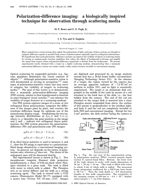
608OPTICS LETTERS/Vol.20,No.6/March15,1995Polarization-difference imaging:a biologically inspired technique for observation through scattering mediaM.P.Rowe and E.N.Pugh,Jr.Institute of Neurological Sciences,University of Pennsylvania,Philadelphia,Pennsylvania19104J.S.Tyo and N.EnghetaMoore School of Electrical Engineering,University of Pennsylvania,Philadelphia,Pennsylvania19104Received August17,1994Many animals have visual systems that exploit the polarization of light,and some of these systems are thought tocompute difference signals in parallel from arrays of photoreceptors optimally tuned to orthogonal polarizations.We hypothesize that such polarization–difference systems can improve the visibility of objects in scattering mediaby serving as common-mode rejection amplifiers that reduce the effects of background scattering and amplifythe signal from targets whose polarization-difference magnitude is distinct from the background.We presentexperimental results obtained with a target in a highly scattering medium,demonstrating that a manmadepolarization-difference system can render readily visible surface features invisible to conventional imaging.Optical scattering by suspended particles(e.g.,fog,rain,plankton)diminishes the visual contrast ofobjects.1–3Although polarization-sensitive vision iswell documented as serving in navigation,1,4,5sometypes of polarization-sensitive vision also may serveto enhance the visibility of targets in scatteringmedia.6,7The goal of this Letter is to demonstratethat a manmade polarization-difference imaging(PDI)system,similar to that hypothesized to functionin some biological visual systems,7,8can enhance thevisibility of target features in a scattering medium.Our PDI system captures images of a scene at twoorthogonal linear polarizations,computes the differ-ence of the images pixel by pixel,and rescales theresultant difference image for optimum use of themonochrome display range.Symbolizing the two im-age intensity distributions as I k͑x,y͒and IЌ͑x,y͒,where͑x,y͒identifies the pixel position in the imageand k andЌindicate two orthogonal linear polar-izations,the PDI system generates the polarization-difference(PD)and polarization-sum(PS)images:PDI͑x,y͒I k͑x,y͒2IЌ͑x,y͒,(1a)PSI͑x,y͒I k͑x,y͒1IЌ͑x,y͒.(1b)If an ideal linear polarizer is used to measure I k andIЌ,then the PS image is equivalent to a polarization-blind image obtained by a conventional imaging sys-tem.In general,PD I depends on the choice of polar-ization axes,whereasPS I does not.The choice of theorthogonal axes will be discussed shortly.The experimental layout is shown in Fig.1.Two incandescent tungsten filament slide projectors backilluminate a sheet of0.64-cm-thick white Plex-iglas attached to a glass tank.The tank is filled with water to which milk is added.The Plexiglas acts as an initial diffuser and the milk as a strong scattering agent.The tank is viewed with a CCD camera(Hamamatsu Model XC-77)equipped with a macro lens(Vivitar Y/C55mm,f2.8).Images are digitized and processed by an image analysis system that has a16-bit frame buffer(accumulator) (Imaging Technology Series151).In the absence of a target,the region viewed by the camera has an average apparent radiance ofϳ7.2W͞(m2sr) uniform to within15%,and its light is essentially unpolarized.The target is an aluminum disk sus-pended in the middle of the tank by means of a rod attached to the back face of the disk,i.e.,the face hidden from the camera.The end of the rod not attached to the target disk is inserted into a clear Plexiglas mount suspended from above;the surface of this mount is perpendicular to the incident light, and both it and the rod are completely invisible to both PDI and conventional imaging.Except for two 1-cm2patches,the disk surface facing the camerais Fig.1.Top:the top view of the experimental setup. A,polarization analyzer;TNLC,twisted nematic liquid crystal;F,narrow-band filter.Bottom:the front view of the tank(drawn to scale)with inside dimensions of 30cm330cm315cm.This tank is filled with water to which5mL of whole milk is added.The measured beam attenuation coefficient for a632.8-nm laser beam is19.7m21.Thus the tank depth isϳ2.9attenuation lengths at this milk concentration.The sensitivity of the imaging system at610nm isϳ4.431027display units͞(quanta s21)(in8-bit display).0146-9592/95/060608-03$6.00/0©1995Optical Society of AmericaMarch15,1995/Vol.20,No.6/OPTICS LETTERS609sandblasted,rendering it nearly Lambertian.These patches,whose relative locations are shown in Fig.1, are a few thousandths of an inch higher than the sandblasted background and have been abraded with emory paper lightly in orthogonal directions—on one patch vertically,and on the other horizontally.The image-forming light from the target surface results from multiple scattering:photons scatter off milk particles to the target surface,and some of these are scattered again toward the camera.Before reaching the camera,the light from the tank passes through a twisted nematic liquid crystal(TNLC;Liquid Crystal Institute,Kent State University.)In its off state, the TNLC rotates the plane of polarization of inci-dent light by90±;when driven,the TNLC passes the incident light with no rotation.After the TNLC,the light passes through a linear polarization analyzer.A narrow-band filter(10nm FWHM,centered at 610nm)eliminates light outside the operating wave-band of the TNLC.When the TNLC is driven,the TNLC͞analyzer passes only light polarized parallel to the analyzer axis,yielding the image I k;when the TNLC is off,the TNLC͞analyzer combination passes light polarized perpendicular to the analyzer axis,yielding IЌ.For the results reported here,the analyzer axis was oriented vertically.Figure2illustrates the application of the PDI sys-tem to the imaging of the aluminum target suspended in diluted milk.Figures2A and2B present the im-ages,I k and IЌ,convolved with a two-dimensional (low-pass)filter.To generate Figs.2A and2B,we summed128consecutive33-ms frames and then di-vided by8.Figures2C and2D presentPSI andPDI, respectively,the sum and difference images.Fig-ures2E and2F re-present the data in images in Figs.2C and2D transformed with affine transfor-mations to use the full intensity range of the dis-play.The abraded patches,which are not visible in Figs.2A–2D,are clearly visible in the transformed PD image(Fig.2F)but practically invisible in the transformed PS image(Fig.2E).Figures2A0–2F0 present numerical plots of average pixel intensities in the pixel region y1#y#y2,as illustrated by the ar-rows shown in Figs.2B,2D,and2F;these plots pro-vide quantitative evidence that supports the qualita-tive conclusion drawn from inspection of the images. The principal factor underlying the enhanced visibility of the two patches in Panel F isthe Fig.2.Application of the PDI system to an aluminum target suspended in diluted milk as illustrated in Fig.1.A,B,The images I k͑x,y͒and IЌ͑x,y͒convolved digitally with a two-dimensional low-pass spatial filter.This filter is roughly a truncated Gaussian,with maximal linear extentϳ5pixel widths;the images of the abraded patches are ഠ80392pixels.The filter removes a periodic high-spatial-frequency artifact produced by the imaging system.Image intensities(ordinates)are expressed in the units of the8-bit display.C,D,PS I͑x,y͒͞2and PD I͑x,y͒1128,respectively [cf.Eqs.(1a)and(1b)];an offset of128was used,because most pixel values of PD I͑x,y͒are near zero and can be positive or negative.E,F,The data of C and D,respectively,but transformed with affine transformations.The transformed values are given by PS I͑x,y͒transa PS͓PS I͑x,y͒2PS I͑x,y͒min͔and by PD I͑x,y͒transa PD͓PD I͑x,y͒2PD I͑x,y͒min͔,where a PS255͓͞PS I͑x,y͒max2PS I͑x,y͒min͔,and similarly for a PD.In E,PS I͑x,y͒max and PS I͑x,y͒min were obtained from the disk region only;the resultant scale factor,a PSഠ6.4,is such that the intensity variation of the disk region occupies the full display range.In F,PD I͑x,y͒max and PD I͑x,y͒min were obtained from the entire image,yielding a PDഠ38.4. Abraded patches,not visible in A–D,are clearly visible in F but practically invisible in E.The vertical bands of pixels in the pixel regions y1#y#y2,as shown by the arrows at the right of panels B,D,and F,were averaged over y to generate numerical plots(as a function of x)shown in A0–F0.610OPTICS LETTERS /Vol.20,No.6/March 15,1995common-mode rejection feature intrinsic to PDI.Given that a target feature may produce a nonzero value of PD I in some region of the image,the system permits extraction of this feature by rejecting intensity common to both polarization axes.This common-mode rejection feature of the PDI system is exhibited in two ways in the images of Fig.2.First,the relatively intense halo of unpolarized light surrounding the disk is eliminated from the PD im-age (cf.Figs.2C 0and 2D 0).Second,the effect of the relatively modest variation (ϳ20%of total display range)across the disk surface is also minimized.This modest intensity variation masks the visibility of the target features in the PS image,and its rejection allows a higher gain to be applied to the PD image than to the PS image (cf.Figs.2E 0and 2F 0).On the basis of the results shown in Fig.2and other data we have obtained,PDI has a gen-eral applicability.First,PDI is quite sensitive to intrinsically small signals.For a particular region of an image,the observed degree of lin-ear polarization (ODLP),defined as ͗ODLP ͘region ͗PD I ͑x ,y ͒͘region ͗͞PS I ͑x ,y ͒͘region ,serves as a dimension-less measure of the PD signal magnitude.For the left patch,͗ODLP ͘10.0164;for the right patch,͗ODLP ͘20.0138.Moreover,in experiments in which we have systematically raised the milk con-centration to degrade the images until the target patches are undetectable,target patches having ͗ODLP ͘&0.01still could be readily seen on in-spection of the PD image (data not shown).The images of many object surfaces in natural environ-ments predictably will have ODLP’s of considerably higher magnitude.9Second,PDI can be generalized readily to scattering environments in which the back-ground itself has nonzero PD I ͑x ,y ͒for a given set of orthogonal polarization axes.Judicious orientation of the analyzer in the PDI system can enhance the PD I of target regions relative to that of the background in the image plane.10Finally,PDI possesses the generally useful qualities of being passive,simple,and potentially very fast.PDI can operate passively in any region of the electromagnetic spectrum in which natural radiation exists.PDI is simple,in that it does not require the use of sophisticated im-age processing techniques;nevertheless,any image processing techniques can be added to,or used in par-allel with,PDI to make it even more effective.PDI is also potentially very fast.In our current setup,it takes 4–5s to obtain each of I k and I Ќ,but this rate limitation is imposed by the low light levels achiev-able with monochromatic light and by the frame rate (30Hz)and limited sensitivity of our imaging sys-tem.With a more-sophisticated system,a higher speed could be achieved with a successive-frame dif-ferencing technique.Furthermore,PDI also can be made very much faster by implementation in a mas-sively parallel system,as nature appears to have done in the retinas of many animals.7,8Other optical imaging techniques also employ po-larization information.3,11–17However,in some of this work,the state of polarization of the illumi-nating light has been known and is typically un-der the experimenters’control.3,11,12In contrast,in PDI the light incident on the target does not have to be polarized,nor need its state of polarization be known or under the control of the imaging system.In other related work 13–17in which there is no con-trol over the polarization of illuminating light either the Stokes parameters have been mapped onto col-orimetric coordinates 13,17or PD I ͑x ,y ͒͞PS I ͑x ,y ͒14–16or some form of percent polarization and polarization angle 16,17has been mapped onto the z axis of a mono-chrome display.Mapping PD I ͑x ,y ͒͞PS I ͑x ,y ͒onto in-tensity confounds the common mode with the signal.In contrast,our technique removes the common mode and allows us to maximize the display of informa-tion that survives the common-mode rejection.The variation and magnitude of PD I are usually less than the variation and magnitude of PS I across the scene.Thus,to use the full dynamic range of a display,higher amplification can be applied to PD I and thus some of the target features not visible to polarization-blind imaging can be observed with PDI.This work is supported by U.S.Department of the Navy Office of Naval Research grant N00014-93-1-0935and,in part,by the University of Pennsylvania Research Foundation.References1.J.N.Lythgoe,The Ecology of Vision (Oxford U.Press,London,1979),pp.112–127.2.S.Q.Duntley,J.Opt.Soc.Am.53,214(1963).3.S.Q.Duntley,in Optical Aspects of Oceanography,N.G.Jerlov and E.Steemann Nielsen,eds.(Academic,New York,1974),pp.135–149.4.K.von Frisch,Experientia 5,142(1949).5.T.H.Waterman,in Vision in Invertebrates,H.Autrum,ed.,Vol.VII/6B of the Handbook of Sen-sory Physiology (Springer-Verlag,New York,1981),pp.281–469.6.J.N.Lythgoe and C.C.Hemmings,Nature (London)213,893(1967).7.D.A.Cameron and E.N.Pugh,Jr.,Nature (London)353,161(1991).8.M.P.Rowe,N.Engheta,S.S.Easter,Jr.,and E.N.Pugh,Jr.,J.Opt.Soc.Am.A 11,55(1994).9.G.P.K¨o nnen,Polarized Light in Nature (Cambridge U.Press,London,1985),pp.74–99.10.J.S.Tyo,University of Pennsylvania,Philadelphia,Pa.(undergraduate senior design project,1994).11.G. D.Gilbert and J. C.Pernicka,in Underwa-ter Photo-Optics,Seminar Proceedings (Society of Photo-Optical Instrumentation Engineers,Belling-ham,Wash.,1966),p.AIII-1.12.B.A.Swartz and J.D.Cummings,Proc.Soc.Photo-Opt.Instrum.Eng.1537,42(1991).13.J.E.Solomon,Appl.Opt.,20,1537(1981).14.G.F.J.Garlick,G.A.Steigmann,and mb,U.S.patent 3,992,571(November 16,1976).15.W.G.Egan,W.R.Johnson,and V.S.Whitehead,Appl.Opt.30,435(1991).16.J.Halajian and H.Hallock,in Proceedings of 8th Sym-posium on Remote Sensing and Environment 1(Envi-ronmental Research Institute of Michigan,Ann Arbor,Mich.,1972),p.523.17.R.Walraven,Proc.Soc.Photo-Opt.Instrum.Eng.112,164(1977).。
polarization
Ey = E2 cos(ωt − βz )
The University of Texas at Dallas
Erik Jonsson School PhoTEC
SNAPSHOT OF PLANE-POLARIZED PLANE WAVE
0
5
Z
10 15 1 0 X -1 0 -1 1
c C. D. Cantrell (03/2004)
2
2
The University of Texas at Dallas
Erik Jonsson School PhoTEC
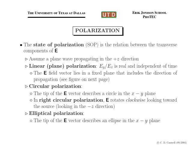
ORTHOGONAL POLARIZATIONS (1) • For a plane wave, there are always 2 orthogonal states of polarization Simplest case: Orthogonal linear polarizations described by unit coordiˆ and y ˆ nate vectors x ˆ·y ˆ=0 ◦ Orthogonality: x ˆ·x ˆ=1=y ˆ·y ˆ ◦ Normalization: x ◦ Example of orthogonally polarized fields: ˆE1 cos(ωt − βz ), E1 = x ˆE2 cos(ωt − βz + δ ) E2 = y The important point: Waves with orthogonal polarizations do not interfere with one another • Example: In a “single-mode” fiber, there are really two modes, one for each of the two orthogonal polarizations These modes don’t have the same group velocity The difference in group velocities leads to polarization-mode dispersion, pulse spreading, and bandwidth limitations
The Refractive Index of Curved Spacetime the Fate of Causality in QED
a r X i v :0707.2303v 2 [h e p -t h ] 29 O c t 2007Preprint typeset in JHEP style -HYPER VERSIONTimothy J.Hollowood and Graham M.Shore Department of Physics,University of Wales Swansea,Swansea,SA28PP,UK.E-mail:t.hollowood@,g.m.shore@ Abstract:It has been known for a long time that vacuum polarization in QED leads to a superluminal low-frequency phase velocity for light propagating in curved spacetime.Assuming the validity of the Kramers-Kronig dispersion relation,this would imply a superluminal wavefront velocity and the violation of causality.Here,we calculate for the first time the full frequency dependence of the refractive index using world-line sigma model techniques together with the Penrose plane wave limit of spacetime in the neighbourhood of a null geodesic.We find that the high-frequency limit of the phase velocity (i.e.the wavefront velocity)is always equal to c andcausality is assured.However,the Kramers-Kronig dispersion relation is violated due to a non-analyticity of the refractive index in the upper-half complex plane,whose origin may be traced to the generic focusing property of null geodesic congruences and the existence of conjugate points.This puts into question the issue of micro-causality,i.e.the vanishing of commutators of field operators at spacelike separated points,in local quantum field theory in curved spacetime.1.IntroductionQuantumfield theory in curved spacetime is by now a well-understood subject.How-ever,there remain a number of intriguing puzzles which hint at deeper conceptual implications for quantum gravity itself.The best known is of course Hawking radia-tion and the issue of entropy and holography in quantum black hole physics.A less well-known effect is the discovery by Drummond and Hathrell[1]that vacuum po-larization in QED can induce a superluminal phase velocity for photons propagating in a non-dynamical,curved spacetime.The essential idea is illustrated in Figure1. Due to vacuum polarization,the photon may be pictured as an electron-positron pair, characterized by a length scaleλc=m−1,the Compton wavelength of the electron. When the curvature scale becomes comparable toλc,the photon dispersion relation is modified.The remarkable feature,however,is that this modification can induce a superluminal1low-frequency phase velocity,i.e.the photon momentum becomes spacelike.Figure1:Photons propagating in curved spacetime feel the curvature in the neighbourhood of their geodesic because they can become virtual e+e−pairs.Atfirst,it appears that this must be incompatible with causality.However, as discussed in refs.[2–4],the relation of causality with the“speed of light”is far more subtle.For our purposes,we may provisionally consider causality to be the requirement that no signal may travel faster than the fundamental constant c defining local Lorentz invariance.More precisely,we require that the wavefront velocity v wf, defined as the speed of propagation of a sharp-fronted wave pulse,should be less than,or equal to,c.Importantly,it may be shown[2,4,5]that v wf=v ph(∞),the high-frequency limit of the phase velocity.In other words,causality is safe even if the low-frequency2phase velocity v ph(0)is superluminal provided the high-frequency limit does not exceed c.This appears to remove the potential paradox associated with a superluminal v ph(0).However,a crucial constraint is imposed by the Kramers-Kronig dispersion relation3(see,e.g.ref.[6],chpt.10.8)for the refractive index,viz.Re n(∞)−Re n(0)=−2ωIm n(ω).(1.1)where Re n(ω)=1/v ph(ω).The positivity of Im n(ω),which is true for an absorptive medium and is more generally a consequence of unitarity in QFT,then implies that Re n(∞)<Re n(0),i.e.v ph(∞)>v ph(0).So,given the validity of the KK dispersion relation,a superluminal v ph(0)would imply a superluminal wavefront velocity v wf= v ph(∞)with the consequent violation of causality.We are therefore left with three main options[4],each of which would have dramatic consequences for our established ideas about quantumfield theory: Option(1)The wavefront speed of light v wf>1and the physical lightcones lie outside the geometric null cones of the curved spacetime,inapparent violation of causality.It should be noted,however,that while this would certainly violate causality for theories in Minkowski spacetime,it could still be possible for causality to be preserved in curved spacetime if the effective metric characterizing the physical light cones defined by v wf nevertheless allow the existence of a global timelike Killing vectorfield. This possible loophole exploits the general relativity notion of“stable causality”[8,9] and is discussed further in ref.[2].Option(2)Curved spacetime may behave as an optical medium ex-hibiting gain,i.e.Im n(ω)<0.This possibility was explored in the context ofΛ-systems in atomic physics in ref.[4], where laser-atom interactions can induce gain,giving rise to a negative Im n(ω)and superluminal low-frequency phase velocities while preserving v wf=1and the KKdispersion relation.However,the problem in extending this idea to QFT is that the optical theorem,itself a consequence of unitarity,identifies the imaginary part of forward scattering amplitudes with the total cross section.Here,Im n(ω)should be proportional to the cross section for e+e−pair creation and therefore positive.A negative Im n(ω)would appear to violate unitarity.Option(3)The Kramers-Kronig dispersion relation(1.1)is itself vio-lated.Note,however,that this relation only relies on the analyticity ofn(ω)in the upper-half plane,which is usually considered to be a directconsequence of an apparently fundamental axiom of local quantumfieldtheory,viz.micro-causality.Micro-causality in QFT is the requirement that the expectation value of the com-mutator offield operators 0|[A(x),A(y)]|0 vanishes when x and y are spacelike separated.While this appears to be a clear statement of what we would understand by causality at the quantum level,in fact its primary rˆo le in conventional QFT is as a necessary condition for Lorentz invariance of the S-matrix(see e.g.ref.[6], chpts.5.1,3.5).Since QFT in curved spacetime is only locally,and not globally, Lorentz invariant,it is just possible there is a loophole here allowing violation of micro-causality in curved spacetime QFT.Despite these various caveats,unitarity,micro-causality,the identification of light cones with geometric null cones and causality itself are all such fundamental elements of local relativistic QFT that any one of these options would represent a major surprise and pose a severe challenge to established wisdom.Nonetheless,it appears that at least one has to be true.To understand how QED in curved spacetime is reconciled with causality,it is therefore necessary to perform an explicit calculation to determine the full frequency dependence of the refractive index n(ω)in curved spacetime.This is the technical problem which we solve in this paper.The remarkable result is that QED chooses option(3),viz.analyticity is violated in curved spacetime.Wefind that in the high-frequency limit,the phase velocity always approaches c,so we determine v wf= 1.Moreover,we are able to confirm that where the background gravitationalfield induces pair creation,γ→e+e−,Im n(ω)is indeed positive as required by unitarity. However,the refractive index n(ω)is not analytic in the upper half-plane,and the KK dispersion relation is modified accordingly.One might think that this implies a violation of microcausality,however,there is a caveat in this line of argument which requires a more ambitious off-shell calculation to settle definitively[7].–3–In order to establish this result,we have had to apply radically new techniques to the analysis of the vacuum polarization for QED in curved spacetime.The original Drummond-Hathrell analysis was based on the low-energy,O(R/m2)effective action for QED in a curved background,L=−1m2 aRFµνFµν+bRµνFµλFνλ+cRµνλρFµνFλρ +···.(1.2) derived using conventional heat-kernel or proper-time techniques(see,for example, [10–14].A geometric optics,or eikonal,analysis applied to this action determines the low-frequency limit of the phase velocity.Depending on the spacetime,the photon trajectory and its polarization,v ph(0)may be superluminal[1,15,16].In subsequent work,the expansion of the effective action to all orders in derivatives,but still at O(R/m2),was evaluated and applied to the photon dispersion relation[11,12,17, 18].However,as emphasized already in refs.[2,3,18],the derivative expansion is inadequate tofind the high-frequency behaviour of the phase velocity.The reason is that the frequencyωappears in the on-shell vacuum polarization tensor only in the dimensionless ratioω2R/m4.The high-frequency limit depends non-perturbatively on this parameter4and so is not accessible to an expansion truncated atfirst order in R/m2.In this paper,we instead use the world-line formalism which can be traced back to Feynman and Schwinger[19,20],and which has been extensively developed in recent years into a powerful tool for computing Green functions in QFT via path integrals for an appropriate1-dim world-line sigma model.(For a review,see e.g.ref.[21].) The power of this technique in the present context is that it enables us to calculate the QED vacuum polarization non-perturbatively in the frequency parameterω2R/m4 using saddle-point techniques.Moreover,the world-line sigma model provides an extremely geometric interpretation of the calculation of the quantum corrections to the vacuum polarization.In particular,we are able to give a very direct interpretation of the origin of the Kramers-Kronig violating poles in n(ω)in terms of the general relativistic theory of null congruences and the relation of geodesic focusing to the Weyl and Ricci curvatures via the Raychoudhuri equations.A further key insight is that to leading order in R/m2,but still exact inω2R/m4, the relevant tidal effects of the curvature on photon propagation are encoded in thef(ωm2Penrose plane-wave limit[22,23]of the spacetime expanded about the original null geodesic traced by the photon.This is a huge simplification,since it reduces the problem of studying photon propagation in an arbitrary background to the much more tractable case of a plane wave.In fact,the Penrose limit is ideally suited to this physical problem.As shown in ref.[24],where the relation with null Fermi normal coordinates is explained,it can be extended into a systematic expansion in a scaling parameter which for our problem is identified as R/m2.The Penrose expansion therefore provides us with a systematic way to go beyond leading order in curvature.The paper is organized as follows.In Section2,we introduce the world-line formalism and set up the geometric sigma model and eikonal approximation.The relation of the Penrose limit to the R/m2expansion is then explained in detail, complemented by a power-counting analysis in the appendix.The geometry of null congruences is introduced in Section3,together with the simplified symmetric plane wave background in which we perform our detailed calculation of the refractive index. This calculation,which is the heart of the paper,is presented in Section4.The interpretation of the result for the refractive index is given in Section5,where we plot the frequency dependence of n(ω)and prove that asymptotically v ph(ω)→1. We also explain exactly how the existence of conjugate points in a null congruence leads to zero modes in the sigma model partition function,which in turn produces the KK-violating poles in n(ω)in the upper half-plane.The implications for micro-causality are described in Section6.Finally,in Section7we make some further remarks on the generality of our results for arbitrary background spacetimes before summarizing our conclusions in Section8.2.The World-Line FormalismFigure2:The loop xµ(τ)with insertions of photon vertex operators atτ1andτ2.–5–In the world-line formalism for scalar QED5the1-loop vacuum polarization is given byΠ1-loop=αT3 T0dτ1dτ2Z V∗ω,ε1[x(τ1)]Vω,ε2[x(τ2)] .(2.1)The loop with the photon insertions is illustrated in Figure(2).The expectation value is calculated in the one-dimensional world-line sigma model involving periodic fields xµ(τ)=xµ(τ+T)with an actionS= T0dτ 15Since all the conceptual issues we address are the same for scalars and spinors,for simplicity we perform explicit calculations for scalar QED in this paper.The generalization of the world-line formalism to spinor QED is straightforward and involves the addition of a further,Grassmann,field in the path integral.For ease of language,we still use the terms electron and positron to describe the scalar particles.6This will require some appropriate iǫprescription.In particular,the T integration contour should lie just below the real axis to ensure that the integral converges at infinity.7In general,one has to introduce ghostfields to take account of the non-trivial measure for the fields, [dxµ(τ)of geometric optics where Aµ(x)is approximated by a rapidly varying exponential times a much more slowly varying polarization.Systematically,we haveAµ(x)= εµ(x)+ω−1Bµ(x)+··· e iωΘ(x).(2.4) We will need the expressions for the leading order piecesΘandε.This will necessitate solving the on-shell conditions to thefirst two non-trivial orders in the expansion in R1/2/ω.To leading order,the wave-vector kµ=ωℓµ,whereℓµ=∂µΘis a null vector (or more properly a null1-form)satisfying the eikonal equation,ℓ·ℓ≡gµν∂µΘ∂νΘ=0.(2.5) A solution of the eikonal equation determines a family or congruence of null geodesics in the following way.9The contravariant vectorfieldℓµ(x)=∂µΘ(x),(2.6) is the tangent vector to the null geodesic in the congruence passing through the point xµ.In the particle interpretation,kµ=ωℓµis the momentum of a photon travelling along the geodesic through that particular point.It will turn out that the behaviour of the congruence will have a crucial rˆo le to play in the resulting behaviour of the refractive index.The general relativistic theory of null congruences is considered in detail in Section3.Now we turn to the polarization vector.To leading order in the WKB approxima-tion,this is simply orthogonal toℓ,i.e.ε·ℓ=0.Notice that this does not determine the overall normalization ofε,the scalar amplitude,which will be a space-dependent function in general.It is useful to splitεµ=Aˆεµ,whereˆεµis unit normalized.At the next order,the WKB approximation requires thatˆεµis parallel transported along the geodesics:ℓ·Dˆεµ=0.(2.7) The remaining part,the scalar amplitude A,satisfies1ℓ·D log A=−εµD·ℓ.(2.9)2Since the polarization vector is defined up to an additive amount of k,there are two linearly independent polarizationsεi(x),i=1,2.Since there are two polarization states,the one-loop vacuum polarization is ac-tually a2×2matrixΠ1-loop ij =αT3 T0dτ1dτ2Z× εi[x(τ1)]·˙x(τ1)e−iωΘ[x(τ1)]εj[x(τ2)]·˙x(τ2)e iωΘ[x(τ2)] .(2.10)In order for this to be properly defined we must specify how to deal with the zero mode of xµ(τ)in the world-line sigma model.Two distinct–but ultimately equiv-alent–methods for dealing with the zero mode have been proposed in the litera-ture[25–29].In thefirst,the position of one particular point on the loop is defined as the zero mode,while in the other,the“string inspired”definition,the zero mode is defined as the average position of the loop:xµ0=1Now notice that the exponential pieces of the vertex operators in(2.1)act as source terms and so the complete action including these ism2S=−T+can always be brought into the formds2=2du dΘ−C(u,Θ,Y a)dΘ2−2C a(u,Θ,Y b)dY a dΘ−C ab(u,Θ,Y c)dY a dY b.(2.14) It is manifest that dΘis a null1-form.The null congruence has a simple description as the curves(u,Θ0,Y a0)forfixed values of the transverse coordinates(Θ0,Y a0).The geodesicγis the particular member(u,0,0,0).It should not be surprising that the Rosen coordinates are singular at the caustics of the congruence.These are points where members of the congruence intersect and will be described in detail in the next section.With the form(2.14)of the metric,onefinds that the classical equations of motion of the sigma model action(2.13)have a solution with Y a=Θ=0whereu(τ)satisfies¨u=−2ωTm2δ(τ).(2.15)More general solutions with constant but non-vanishing(Θ,Y a)are ruled out by the constraint(2.12).The solution of(2.15)is˜u(τ)=−u0+ 2ωT(1−ξ)τ/m20≤τ≤ξ2ωTξ(1−τ)/m2ξ≤τ≤1.(2.16)where the constantu0=ωTξ(1−ξ)/m2(2.17) ensures that the constraint(2.12)is satisfied.The solution describes a loop which is squashed down onto the geodesicγas illustrated in Figure(3).The electron and positron have to move with different world-line velocities in order to accommodate the fact that in generalξis not equal to1Now that we have defined the Rosen coordinates and found the classical saddle-point solution,we are in a position to set up the perturbative expansion.The idea is to scale the transverse coordinatesΘand Y i in order to remove the factor of m2/T in front of the action.The affine coordinate u,on the other hand,will be left alone since the classical solution˜u(τ)is by definition of zeroth order in perturbation theory. The appropriate scalings are precisely those needed to define the Penrose limit[22]–in particular we closely follow the discussion in[23].The Penrose limit involvesfirst a boost(u,Θ,Y a)−→(λ−1u,λΘ,Y a),(2.18) whereλ=T1/2/m,and then a uniform re-scaling of the coordinates(u,Θ,Y a)−→(λu,λΘ,λY a).(2.19) As argued above,it is important that the null coordinate along the geodesic u is not affected by the combination of the boost and re-scaling;indeed,overall(u,Θ,Y a)−→(u,λ2Θ,λY a).(2.20) After these re-scalings,the sigma model action(2.13)becomesS=−T+1m2Θ(ξ)+ωT4 10dτ 2˙u˙Θ−C ab(u,0,0)˙Y a˙Y b −ωT m2Θ(0)+···.(2.22) The leading order piece is precisely the Penrose limit of the original metric in Rosen coordinates.Notice that we must keep the source terms because the combination ωT/m2,or more precisely the dimensionless ratioωR1/2/m2,can be large.However, there is a further simplifying feature:once we have shifted the“field”about the clas-sical solution u(τ)→˜u(τ)+u(τ),it is clear that there are no Feynman graphs with-out externalΘlines that involve the vertices∂n u C ab(˜u,0,0)u n˙Y a˙Y b,n≥1;hence, we can simply replace C ab(˜u+u,0,0)consistently with the background expression C ab(˜u,0,0).This means that the resulting sigma model is Gaussian to leading order in R/m2:S(2)=14 10dτC ab(˜u,0,0)˙Y a˙Y b,(2.23)wherefinally we have dropped the˙u˙Θpiece since it is just the same as inflat space and the functional integral is normalized relative toflat space.This means that all the non-trivial curvature dependence lies in the Y a subspace transverse to the geodesic.10It turns out that the Rosen coordinates are actually not the most convenient co-ordinates with which to perform explicit calculations.For this,we prefer Brinkmann coordinates(u,v,y i).To define these,wefirst introduce a“zweibein”in the subspace of the Y a:C ab(u)=δij E i a(u)E j b(u),(2.24) with inverse E a i.This quantity is subject to the condition thatΩij≡dE iadE ia2E a j.(2.29)du2We have introduced these coordinates at the level of the Penrose limit.However, they have a more general definition for an arbitrary metric and geodesic.They are in fact Fermi normal coordinates.These are“normal”in the same sense as the more common Riemann normal coordinates,but in this case they are associated to the geodesic curveγrather than to a single point.This description of Brinkmann coordinates as Fermi normal coordinates and their relation to Rosen coordinates and the Penrose limit is described in detail in ref.[24].In particular,this reference givestheλexpansion of the metric in null Fermi normal coordinates to O(λ2).To O(λ) this isds2=2du dv−R iuju y i y j du2−dy i2+λ −2R uiuv y i v du2−43R uiuj;k y i y j y k du2 +O(λ2),(2.30)which is consistent with(2.28)since R iuju=−h ij for a plane wave.It is worth pointing out that Brinkmann coordinates,unlike Rosen coordinates,are not singular at the caustics of the null congruence.One can say that Fermi normal coordinates (Brinkmann coordinates)are naturally associated to a single geodesicγwhereas Rosen coordinates are naturally associated to a congruence containingγ.In Brinkmann coordinates,the Gaussian action(2.23)for the transverse coordi-nates becomesS(2)=−12m2Ωij y i y j τ=ξ−ωTexplicitly.In doing so,we discover many surprising features of the dispersion relation that will hold in general.The symmetric plane wave metric is given in Brinkmann coordinates by(2.28), with the restriction that h ij is independent of u.This metric is locally symmetric in the sense that the Riemann tensor is covariantly constant,DλRµνρσ=0,and can be realized as a homogeneous space G/H with isometry group G.12With no loss of generality,we can choose a basis for the transverse coordinates in which h ij is diagonal:h ij y i y j=σ21(y1)2+σ22(y2)2.(3.1) The sign of these coefficients plays a crucial role,so we allow theσi themselves to be purely real or purely imaginary.For a general plane-wave metric,the only non-vanishing components of the Rie-mann tensor(up to symmetries)areR uiuj=−h ij(u).(3.2) So for the symmetric plane wave,we have simplyR uu=σ21+σ22,(3.3)R uiui=−σ2iand for the Weyl tensor,1C uiui=−σ2i+12Notice that,contrary to the implication in ref.[4,18],the condition that the Riemann tensor is covariantly constant only implies that the spacetime is locally symmetric,and not necessarily maximally symmetric[13,23].A maximally symmetric space has Rµνρσ=1plane wave background,then explain how the key features are described in the gen-eral theory of null congruences.The geodesic equations for the symmetric plane wave(2.28),(3.1)are:¨u=0,¨v+2˙u2i=1σ2i y i˙y i=0,¨y i+˙u2σ2i y i=0.(3.5)We can therefore take u itself to be the affine parameter and,with the appropriate choice of boundary conditions,define the null congruence in the neighbourhood of, and including,γas:v=Θ−122i=1σi tan(σi u+a i)y i2.(3.9)The tangent vector to the congruence,defined asℓµ=gµν∂νΘ,is therefore ℓ=∂u+1The polarization vectors are orthogonal to this tangent vector,ℓ·εi=0,and are further constrained by(2.9).Solving(2.7)for the normalized polarization(one-form) yields13ˆεi=dy i+σi tan(σi u+a i)y i du.(3.11) The scalar amplitude A is determined by the parallel transport equation(2.8),from which we readilyfind(normalizing so that A(0)=1)A=2i=1 cos(σi u+a i)(3.12)The null congruence in the symmetric plane wave background displays a number of features which play a crucial role in the analysis of the refractive index.They are best exhibited by considering the Raychoudhuri equation,which expresses the behaviour of the congruence in terms of the optical scalars,viz.the expansionˆθ, shearˆσand twistˆω.These are defined in terms of the covariant derivative of the tangent vector as[30]:ˆθ=1112Rµνℓµℓν,Ψ0=Cµρνσℓµℓνmρmσ.14As demonstrated in refs.[31],the effectof vacuum polarization on low-frequency photon propagation is also governed by the two curvature scalarsΦ00andΨ0.Indeed,many interesting results such as the polarization sum rule and horizon theorem[31,32]are due directly to special properties ofΦ00andΨ0.As we now show,they also play a key rˆo le in the world-line formalism in determining the nature of the full dispersion relation.√2R uu=1 2(C u1u1−C u2u2)=1By its definition as a gradientfield,it is clear that D[µℓν]=0so the null con-gruence is twist-freeˆω=0.The remaining Raychoudhuri equations can then be rewritten as∂u(ˆθ+ˆσ)=−(ˆθ+ˆσ)2−Φ00−|Ψ0|,∂u(ˆθ−ˆσ)=−(ˆθ−ˆσ)2−Φ00+|Ψ0|.(3.15) The effect of expansion and shear is easily visualized by the effect on a circular cross-section of the null congruence as the affine parameter u is varied:the expansionˆθgives a uniform expansion whereas the shearˆσproduces a squashing with expansion along one transverse axis and compression along the other.The combinationsˆθ±ˆσtherefore describe the focusing or defocusing of the null rays in the two orthogonal transverse axes.We can therefore divide the symmetric plane wave spacetimes into two classes, depending on the signs ofΦ00±|Ψ0|.A Type I spacetime,whereΦ00±|Ψ0|are both positive,has focusing in both directions,whereas Type II,whereΦ00±Ψ0 have opposite signs,has one focusing and one defocusing direction.Note,however, that there is no“Type III”with both directions defocusing,since the null-energy condition requiresΦ00≥0.For the symmetric plane wave,the focusing or defocusing of the geodesics is controlled byeq.(3.6),y i=Y i cos(σi u+a i).Type I therefore corresponds toσ1and σ2both real,whereas in Type II,σ1is real andσ2is pure imaginary.The behaviour of the congruence in these two cases is illustrated in Figure(4).1y21y2Figure4:(a)Type I null congruence with the special choiceσ1=σ2and a1=a2so that the caustics in both directions coincide as focal points.(b)Type II null congruence showing one focusing and one defocusing direction.To see this explicitly in terms of the Raychoudhuri equations,notefirst that the curvature scalarsΦ00−|Ψ0|=σ21,Φ00+|Ψ0|=σ22are simply the eigenvalues of h ij.The optical scalars areˆθ=−12 σ1tan(σ1u+a1)−σ2tan(σ2u+a2) (3.16)and we easily verify∂uˆθ=ˆθ2−ˆσ2−12(σ21−σ22).(3.17)It is clear that provided the geodesics are complete,those in a focusing direction will eventually cross.In the symmetric plane wave example,with y i=Y i cos(σi u+ a i),these“caustics”occur when the affine parameterσi u=π(n+115This does not necessarily mean that the conjugate points are joined by more than one actual geodesic,only that an infinitesimal deformation ofγter we shall see that the existence of conjugate points relies on the existence of zero modes of a linear problem.Conversely,the existence of a geodesic other thanγjoining p and q does not necessarily mean that p and q are conjugate[8,33].16Whether these deformed geodesics become actual geodesics is the question as to whether they lift from the Penrose limit to the full metric.4.World-line Calculation of the Refractive IndexIn this section,we calculate the vacuum polarization and refractive index explicitly for a symmetric plane wave.As we mentioned at the end of Section 2,the explicit calculations are best performed in Brinkmann coordinates.We will need the expres-sions for Θand εi for the symmetric plane wave background:these are in eqs.(3.9),(3.11)and (3.12).From these,we have the following explicit expression for the vertex operator 17V ω,εi [x µ(τ)]= ˙y i +σi tan(σi ˜u +a i )˙˜u y i 2 j =1 cos(σj ˜u +a j )×exp iω v +1410dτ ˙y i 2−˙˜u 2σ2i yi 2 −ωT σi −det g [x (τ)]which can be exponenti-ated by introducing appropriate ghosts [25–29].However,in Brinkmann coordinatesafter the re-scaling (2.27),det g =−1+O (λ)and so to leading order in R/m 2the determinant factor is simply 1and so plays no rˆo le.The same conclusion would not be true in Rosen coordinates.The y i fluctuations satisfy the eigenvalue equation¨y i+˙˜u 2σ2i y i −2ωT σi 17Notice that at leading order in R/m 2we are at liberty to replace u (τ)by its classical value ˜u (τ).The argument is identical to the one given in Section 2.。
Lamb Shift of Muonic Deuterium and Hydrogen
a r X i v :p h y s i c s /0507019v 1 [p h y s i c s .a t o m -p h ] 4 J u l 2005Lamb Shift of Muonic Deuterium and Hydrogen E.BorieForschungszentrum Karlsruhe,Institut f¨u r Hochleistungsimpuls and Mikrowellentechnik (IHM),Hermann-von-Helmholtzplatz 1,76344Eggenstein-Leopoldshafen,Germany Abstract My previous calculations of the Lamb shift in muonic hydrogen are reviewed and compared with other work.In addition,numerical results for muonic deuterium are presented.Introduction The energy levels of muonic atoms are very sensitive to effects of quantum electrodynamics (QED),nuclear structure,and recoil,since the muon is about 206times heavier than the electron [1].A number of theoretical analyses of the Lamb shift (the 2p-2s transition)in light muonic atoms have been published [2,3,4,5,6,15,7,9,16],most recently in view of a proposed measurement of the Lamb shift im muonic hydrogen [8].The present paper repeats the independent recalculation of some of the most important effects [3]and extends the numerical calculations to the case of muonic deuterium,including effects that were not considered previously [10].Muonic deuterium is in many ways similar to muonic hydrogen,but there are some differences.In addition to the different mass the deuteron has spin 1and both magnetic and quadrupole moments.In the numerical calculations the fundamental constants from CODATA 2002([11]):α−1, c ,m µ,m e ,m u =137.0359991,197.32697MeV ·fm,105.658369MeV,0.5109989MeV,931.5050MeV,respectively Also,the following properties of the proton and deuteron were used:m p =938.272MeV/c 2,R p =0.875±0.007fm (other recent values are discussed below)and µp =2.79285µN .Also,m d =1875.613MeV/c 2,R d =2.139±0.003fm and µd =0.85744µN =0.307012µp .([11])The deuteron has spin 1and thus has both magnetic and quadrupole moments.The quadrupole moment of the deuteron is taken to be Q =0.2860(15)fm 2[12,13,14].Vacuum PolarizationThe most important QED effect for muonic atoms is the virtual production and anni-hilation of a single e +e −pair It has as a consequence an effective interaction of order αZαwhich is usually called the Uehling potential ([17,18].This interaction describes the most important modification of Coulomb’s law.Numerically it is so important that it should not be treated using perturbation theory;instead the Uehling potential should be added to the nuclear electrostatic potential before solving the Dirac equation.However,a perturbative treatment is also useful in the case of very light atoms,such as hydrogen.However,unlike some other authors,we prefer to use relativistic(Dirac)wave functions to describe the muonic orbit.Since these contributions have been extensively discussed in the literature[1,2,3,4](among others),there is no need to go into detail here.The results,calculated as the expectation value of the Uehling potential using point-Coulomb Dirac wave functions with reduced mass are,for muonic deuterium:R d=2.139fm2p1/2−2s1/22p3/2−2s1/2227.6577227.66351.66622 1.66626point nucleus2p1/2−2s1/22p3/2−2s1/2 Uehling205.0199205.0250Kaellen-Sabry 1.50807 1.50811The effect offinite proton size calculated here can be parametrized as-0.0109 r2 .How-ever higher iterations can change these results.The contribution due to two and three iterations have been calculated by[4]and[23],respectively,giving a total of0.151meV. An additional higher iteration includingfinite size and vacuum polarization is given in ref.[4](equations(66)and(67))and ref.[2](equations(264)and(268)).These amount to -0.0164 r2 .The best way to calculate this would be an accurate numerical solution of the Dirac equation in the combined Coulomb-plus Uehling potential.The mixed muon-electron vacuum polarization correction([21,2])is0.00007meV for hydrogen and0.00008meV for deuterium.The Wichmann-Kroll contribution was calculated using the parametrization for the potential given in[1].The result obtained for hydrogen is-0.00103meV,consistent with that given in[2].For deuterium,the contribution is-0.00111meV.The equivalent potential for the virtual Delbr¨u ck effect was recomputed from the Fourier transform given in[22]and[1].The resulting potential was checked by reproducing previously calculated results for the2s-2p transition in muonic Helium,and the3d-2p transitions in muonic Mg and Si.The result for hydrogen is+(0.00135±0.00015)meV, and for deuterium it is+(0.00147±0.00016)meV.As in the case of muonic helium, this contribution very nearly cancels the Wichmann-Kroll contribution.The contribution corresponding to three photons to the muon and one to the proton should be analogous to the light by light contribution to the muon anomalous moment;to my knowledge, the corresponding contribution to the muon form factor has never been calculated.It will be comparable to the other light by light contributions.This graph was included in contributions to the muon’s anomalous magnetic moment;the contribution to the muon form factor is one of the most significant unknown corrections.The sixth order vacuum polarization corrections to the Lamb shift in muonic hydrogen have been calculated by Kinoshita and Nio[23].Theirresultforthe 2p-2stransition(in hydrogen)is ∆E (6)=0.120045·(αZ )2·m rα3αZm r 2 r 3 (2)+(αZ )2(F REL +m 2r F NR ) (1)where r 2 is the mean square radius of the proton.For muonic hydrogen,the coef-ficient of r 2 is 5.1975(meV fm −2),giving an energy shift (for the leading term)of (3.979±0.076)meV if the proton rms radius is 0.875fm.Other values of the proton radius that have been reported recently in the literature are 0.880fm [25]and (0.895±0.018fm)[26].The second term in Eq.(1)contributes -0.0232meV for a dipole form factor and -0.0212meV for a Gaussian form factor.The parameters were fitted to the proton rms radius.This can be written as -0.0347 r 2 3/2or -0.0317 r 2 3/2.This differs slightly from the value given by Pachucki [5].The model dependence introduces an uncertainty about ±0.002meV.The remaining terms contribute 0.00046meV.This estimate includes all of the terms given in [24],while other authors [5]give only some of them.Clearly theneglected terms are not negligible.There is also a contribution of-3·10−6meV to the binding energy of the2p1/2-level,and a recoil correction of0.013meV to the binding energy of the2s-level.Pachucki[5]has estimated a correction similar to the second term(proportional to r3 (2))in Eq.(1).Since the logarithmic terms in the two-photon correction withoutfinite size(see below)also seem to be suspect,this correction requires further investigation. In particular,the parametrization of the form factors used in any calculation should reproduce the correct proton radius.For muonic deuterium,the main contribution amounts to-6.0732 r2 =-(27.787±0.078)meV.Depending on the model,the term proportional to r3 (2)gives a contribution of0.382meV or0.417meV.As mentioned previously,thefinite-size contributions to vacuum polarization in muonic hydrogen can be parametrized as−0.0109 r2 −0.0164 r2 ,giving a total of−0.0273 r2 or-0.0209(6)meV if the proton radius is0.875fm.For deuterium.only the contribution corresponding to thefirst term of the sum(−0.0129 r2 )has been calculated.The contribution due to nuclear polarization(in hydrogen)has been calculated by Rosenfelder[29]to be0.017±0.004meV,and by Pachuki[5]to be0.012±0.002meV. Other calculations[30,31]give intermediate values(0.013meV and0.016meV,respec-tively).The value appearing in table2is an average of the three most recent values,with the largest quoted uncertainty,which is probably underestimated.Relativistic RecoilAs is well-known,the center-of-mass motion can be separated exactly from the relative motion only in the nonrelativistic limit.Relativistic corrections have been studied by many authors,and will not be reviewed here.The relativistic recoil corrections summa-rized in[1]include the effect offinite nuclear size to leading order in mµ/m N properly.Up to now this method has been used to treat recoil corrections to vacuum polarization only in the context of extensive numerical calculations that include the Uehling potential in the complete potential,as described in[1].They can be included explicitly,as a perturbation correction to point-Coulomb values.Recall that(to leading order in1/m N), the energy levels are given byE=E r−B202mNh(r)+2B0P1(r) (2)where E r is the energy level calculated using the reduced mass and B0is the unperturbed binding energy.Alsoh(r)=−P1(r)(P1(r)+13rQ2(r)[P1(r)+Q4(r)/r3](3)HereP1(r)=4παZ ∞r r′ρ(r′)dr′=−V(r)−rV′(r)(4)Q2(r)=4παZ r0r′2ρ(r′)dr′=r2V′(r)Q4(r)=4παZ r0r′4ρ(r′)dr′An effective charge densityρV P for vacuum polarization can be derived from the Fourier transform of the Uehling potential.Recall that(for a point nucleus)V Uehl(r)=−αZ3π·χ1(2m e r)=−(αZ)2αz2·1+1π ∞0q2·j0(qr)3π·∞1dz(z2−1)1/22z2 2q2+4m2e z2dq =23π(2m e)χ0(2m e r)Q2(r)=αZ 1+2α3π ∞1dz(z2−1)1/22z2· 2q2+4m2e z2(6qr−(qr)3)cos(qr)+(3(qr)2−6)sin(qr)(deuterium).To obtain the full relativistic and recoil corrections,one must add thedifference between the expectation values of the Uehling potential calculated with rel-ativistic and nonrelativistic wave functions,giving a total correction of0.0166meV formuonic hydrogen.This is in quite good agreement with the correction of.0169meVcalculated by Veitia and Pachucki[33].The treatment presented here has the advantage of avoiding second order perturbation theory.For deuterium,one obtains a total correctionof0.0179meV.The review by Eides et al.[2]gives a better version of the two photon recoil(Eq.136)than was available for the review by Borie and G.Rinker[1].Evaluating this expressionfor muonic hydrogen gives a contribution of-0.04497meV to the2p-2s transition in hydrogen and-0.02656meV in deuterium.Higher order radiative recoil corrections givean additional contribution(in hydrogen)of-0.0096meV[2].However,some of thecontributions to the expressions given in[2]involve logarithms of the mass ratio mµ/m N. Logarithms can only arise in integrations in the region from mµto m N;in this regionthe effect of the nuclear form factor should not be neglected.Pachucki[4]has estimated afinite size correction to this of about0.02meV,which seems to be similar to the termproportional to r3 (2)given in Eq.(1)as calculated in the externalfield approximation by Friar[24].This two-photon correction requires further investigation.In particular, the parametrization of the form factors used in any calculation should reproduce thecorrect proton radius.Also the relationship among the different contributions needs to be specified more clearly.An additional recoil correction for states withℓ=0has been given by[34](see also[2]).It is∆E n,ℓ,j=(αZ)4·m3rκ(2ℓ+1) (6)When evaluated for the2p-states of muonic hydrogen,onefinds a contribution to the 2p-2s transition energy of0.0575meV for the2p1/2state and-0.0287meV for the2p3/2 state in hydrogen(0.0168meV for the2p1/2state and-0.0084meV for the2p3/2state in deuterium)Afinal point about recoil corrections is that in the case of light muonic atoms,the mass ratio mµ/m N is considerably larger than the usual perturbation expansion parameterαZ. Contributions of higher order in the mass ratio could be significant.Muon Lamb ShiftFor the calculation of muon self-energy and vacuum polarization,the lowest order(one-loop approximation)contribution is well-known,at least in perturbation theory.Including also muon vacuum polarization(0.0168meV)and an extra term of order(Zα)5as given in[2]:which contributes-0.00443meV,onefinds a contribution of-0.66788meV for the 2s1/2−2p1/2transition and-0.65031meV for the2s1/2−2p3/2transition.For deuterium, the corresponding contributions are given by-0.77462meV for the2s1/2−2p1/2transi-tion and-0.75512meV for the2s1/2−2p3/2transition.The second order calculation indeuterium includes muonic vacuum polarization(0.01968meV);the extra term of order (Zα)5as given in[2],contributes-0.00518meV.These results,and the higher order corrections[1,21]can be summarized asTransition2p1/2−2s1/22p3/2−2s1/2m2µ· ∇2V m2µF′1(0)+aµ2m2µ 2dr L· σµwhere F2(0)=aµ;the higher order contributions(fourth and sixth)can be taken from the well-known theory of the muon’s anomalous magnetic moment:F2(0)=aµ=α/2π+0.7658(α/π)2+24.05(α/π)3.The fourth order contribution to F′1(0)is0.46994(α/π)2+2.21656(α/π)2=2.68650(α/π)2[1].The sixth order contributions to F′1(0)that involve electron vacuum polarization loops(especially the light-by-light graph) might contribute at an experimentally significant level,but have not been calculated.Summary of contributions for muonic hydrogenUsing the fundamental constants from the CODATA2002([11])onefinds the transition energies in meV in table2.Here the main vacuum polarization contributions are given for a point nucleus,using the Dirac equation with reduced mass.Some uncertainties have been increased from the values given by the authors,as discussed in the text.Thefinite size corrections for hydrogen up to order(αZ)5can be parametrized as 5.1975 r2 +0.0109 r2 +0.0164 r2 +0.0347 r3 (2).The various contributions are dis-cussed in the text.Contribution Value(meV)Uncertainty(meV)recoil[2](eq136)-0.04497recoil,higher order[2]-0.0096recoil,finite size[24]0.0130.001recoil correction to VP[1]-0.0042additional recoil[34]0.0575nuclear size(R p=0.875fm)0.007fmmain correction[24]-3.9790.076order(αZ)5[24]0.02320.002order(αZ)6[24]-0.0005correction to VP-0.0083polarization0.0150.004parametrized as6.0732 r2 +0.0129 r2 +0.0409 r3 (2),although not all contributions to the effect of finite size on the vacuum polarization correction are included.Contribution Value(meV)Uncertainty(meV)recoil[2](eq136)-0.02656recoil,higher order[2]?recoil,finite size[24]0.0190.003recoil correction to VP[1]-0.0048additional recoil[34]0.0168nuclear size(R d=2.139fm)0.003fmmain correction[24]-27.7870.078order(αZ)5[24]0.04000.018order(αZ)6[24]-0.0045correction to VP-0.0592polarization?Hydrogen Deuterium Dirac8.415648.86430Uehling(VP)0.00500.00575K¨a llen-Sabry 0.000040.00005Recoil (Eq.(6))-0.0862-0.02522m µ1dr1+a µm µ L · s 1(7)This can be rearranged to give the well-known form for spin 1/2particles with an anomalous magnetic moment,namely−1dr ·1+a µ+(a µ+1/2)m N /m µm N m µ+12m 2r −12m 21dr 1+κ2/Z m 2 L · s 2Usually one writes Z +κ2m p where µ2is the magnetic moment of the nucleus in units of nuclear magnetons (µN =e/2m p ).A value of µd =0.85744µN =0.307012µp corresponds to κd =0.714.V s 1,s 2=2(1+a µ)µ2r dV 3∇2V s 1· s 2V Q=−αQ 1dr 3 s2·ˆr s2·ˆr− s2· s2with Q in units of1/m22.Thequadrupolemomentof thedeuteronis taken to beQ=0.2860(15)fm2[12,13,14].In other units,onefinds Q=25.84/m2d=7.345×10−6MeV−2.Note that V L,s1describes thefine structure,while the hyperfine structure is described(in perturbation theory)by the expectation values of V L,s2,V s1,s2,and V Q(where appli-cable).The Uehling potential has to be included in the potential V(r).For states withℓ>0 in light atoms,and neglecting the effect offinite nuclear size,we may take1dr =αZ3π ∞1(z2−1)1/22z2·(1+2m e rz)·e−2m e rz dz (8)which is obtained from the Uehling potential[17,18]by differentiation.Then,assuming that it is sufficient to use nonrelativistic point Coulomb wave functions for the2p state, onefinds 1r3 2p·(1+ε2p)whereε2p=2αz2·1+1(1+az)2+2az4mµm N 1dr 2p·(1+κ) 2(1+x p)δjj′(F(F+1)−11/4)+6ˆjˆj′(C F1(1+aµ)−2(1+x)) ℓF112j ℓF112j′ (10) whereˆj=√2m p(1+κp)=0.09245represents a recoil correction due to Thomas precession[7,34,35].The correction due to vacuum polarization(Eq.(9))should be applied to the HFS shifts of the2p-states.As has been known for a long time[7,16,4,35],the states with total angular momentum F=1are a superposition of the states with j=1/2and j=3/2.Let thefine structure splitting be denoted byδ=E2p3/2−E2p1/2=8.352meV,and letβp=(αZ)4m3r1/21/2(β′/8)(2+x p+aµ)[−δF,0+1/3δF,1]3/23/2δ+(β′/4)(4+5x d−aµ)[−1/12δF,1+1/20δF,2]3/21/2(β′/24)(1+2x p−aµ)[√Then for the2p-level with j=j′=1/2and F=0,the energy shift is given by −(β′/8)(2+x p+aµ)=-5.971meV,and for the2p-level with j=j′=3/2and F=2, the energy shift is given byδ+(β′/80)(4+5x p−aµ)=9.6243meV.For the2p-levels with F=1the corresponding matrix has to be diagonalized.The resulting numerical values for the eigenvalues are(∆±R)/2=1.846meV and6.376meV, where∆=δ−β′(x p−aµ)/16R2=[δ−β′(1+7x p/8+aµ/8)/6]2+(β′)2(1+2x p−aµ)2/288Hyperfine structure of the2p-state in muonic deuteriumFor the2p state,the matrix elements of the magnetic hyperfine structure have been given by Brodsky and Parsons[35].For hydrogen they are the same as those calculated above. Here the Uehling potential will be included in the expectation value of1dras discussed above.LetβD=16(1+κd)(αZm r/n)3ℓ(ℓ+1)(2ℓ+1)=(1+κd)1/21/2(βD/6)(2+x d+aµ)[−δF,1/2+1/2δF,3/2]3/23/2δ+(βD/4)(4+5x d−aµ)[−1/6δF,1/2−1/15δF,3/2+1/10δF,5/2] 3/21/2(βD/48)(1+2x d−aµ)[√5δF,3/2]where x d=(m2µ/m d m r)(κd/(1+κd))=0.0248.For the evaluation of the contributions of the quadrupole HFS,letǫQ=αQ 1drFor a point Coulomb potential,and the2p-state,ǫQ=αQ(Zαm r)3/24=0.43243meV. The quadrupole interaction results in energy shifts ofj j′Energy2δF,1/2−1/√As mentioned before,the Uehling potential has to be included in the potential V(r). For states withℓ>0in light atoms,this can be taken into account by multiplyingβD andǫQ by(1+ε2p)whereε2p is given by Eq.(9).With a numerical value ofε2p=0.000391 for muonic deuterium,the value ofǫQ is increased to0.43440meV and the value ofβD is increased toβ′D=4.0922meV.Then for the2p-level with j=j′=3/2and F=5/2,the energy shift is given by δ+ǫQ/5+(β′D/40)(4+5x d−aµ)=9.373meV.For the2p-levels with F=1/2and F=3/2,the corresponding matrices have to be diagonalized.The resulting numerical values for the eigenvalues are,for F=1/2,-1.3834meV and8.5974meV;for F=3/2they are0.6856meV and 8.2410meV.Hyperfine structure of the2s-state:in an ns state with j=1/2isThe expectation value of V s1s22µ2α(αZ)3m3r∆E ns==3n3mµm2·(1+κ2)·(1+aµ)=(8/n3)βp·(1+aµ)=(8/n3)×22.8332meV (see,for example[2],Eq.(271,277)).The numerical value was calculated for hydrogen. For deuterium,with s2=1,the corresponding hyperfine splitting is2(αZ)4m3r∆E ns=As was shown in[7,2],the energy shift of the2s-state in muonic hydrogen is given by:∆E2s=β·(1+aµ)·(1+εV P+εvertex+εBreit+εF S,rec)·[δF1−3δF0]/4(11) The corrections due to QED effects,nuclear size and recoil are analogous for muonic deuterium.The QED corrections have been discussed by Borie[3,7,16](see also[38]),and are given in Appendix2.The correction due tofinite size and recoil have been given in[4]as-0.145meV,while a value of-0.152meV is given in[42].Ref.[4]also gives a correction as calculated by Zemach([40])equal to-0.183meV,but claims that this correction does not treat recoil properly.The Zemach correction is equal toεZem=−2αZm r r (2)where r (2)is given in[7,24,41].Using the value r (2)=1.086±0.012fm from[41], givesεZem=−0.00702,and a contribution of of-0.1742meV to the hyperfine splitting of the2s state.Including this,but not other recoil corrections to the hyperfine structure of the2s-state gives a total splitting of22.7806meV.Additional higher order corrections calculated in Ref.[42]amount to a total of-0.0003meV and are not included here.It would be very desirable to understand the reasons for the discrepancy between references[4]and[42]in the calculations of this effect.Also,since the Zemach radius seems to be sensitive to details of the electric and magnetic charge distributions[41], evaluations performed with a dipole-type form factor may not be good enough.This point requires further invesigation.For muonic deuterium,the coefficient of r (2)is-0.007398fm−1,giving,withr (2)=2.593±0.016fm from[41],εZem=−0.01918±0.00012.The total hyperfine splitting of the2s-state of muonic deuterium,including all correc-tions,is3∆E2s=Transition Energy shift in meV2p1/2−2s1/2 2.6552p3/2−2s1/212.6364p1/2−2s1/2 4.7244p3/2−2s1/212.2802p1/2−4s1/2-3.4032p3/2−4s1/2 6.5784p1/2−4s1/2-1.3346p3/2−4s1/2 6.2226p3/2−4s1/27.354Table6:Fine-and hyperfine contributions to the Lamb shift in muonic deuterium.Tables5and6give the contributions to the transition energies due tofine and hyperfine structure.Summary of contributions and ConclusionsThe most important contributions to the Lamb shift in muonic hydrogen,including hyperfine structure,have been independently recalculated.A new calculation of some terms that were omitted in the most recent literature,such as the virtual Delbr¨u ck effect [22]and an alternative calculation of the relativistic recoil correction have been presented.Numerically the results given in table2add up to a total correction of (206.032(6)-5.225 r2 +0.0347 r2 3/2)meV=202.055±0.12meV.(for the value of the proton radius from[11]).As is well known,most of the uncertainty arises from the uncertainty in the proton radius.Numerical results were also given for muonic deuterium.The total correction is (228.573(6)-6.086 r2 +0.0409 r2 3/2)meV=200.767±0.09meV.The complete depen-dence on the deuteron radius is uncertain since contributions from iteration of the po-tential are not included.Also,some other contributions are not included,as indicated in table3AcknowledgmentsThe author wishes to thank M.Eides,E.-O.Le Bigot and F.Kottmann for extensive email correspondence regarding this work.References[1]E.Borie,G.A.Rinker,Rev.Mod.Phys.54,67(1982)[2]M.I.Eides,H.Grotch,V.A.Selyuto,Physic Reports,342,63-261(2001)[3]E.Borie,Phys.Rev.A71,032508(2005)[4]K.Pachucki,Phys.Rev.A53,2092(1996)[5]K.Pachucki,Phys.Rev.A60,3593(1999)[6]E.Borie,Z.Phys.A275,347(1975)[7]E.Borie,Z.Phys.A278,127(1976)[8]F.Kottmann et al.,Hyperf.Int.138,55(2001)[9]A.di Giacomo,Nucl.Phys.B11,411(1969)[10]G.Carboni,Lett.Nuov.Cim.7,160(1973)[11]P.J.Mohr,B.N.Taylor,Rev.Mod.Phys.77,1(2005)[12]J.L.Friar,Can.J.Phys.80,1337(2002)[13]R.V.Reid,M.L.Vaida,Phys.Rev.Lett.29,494(1972);(E)34,1064(1975)[14].D.M.Bishop,L.M.Cheung,Phys.Rev.A20,381(1979)[15]E.Borie,G.A.Rinker,Phys.Rev.A18,324(1978)[16]E.Borie,Z.Phys.A297,17(1980)[17]E.A.Uehling,Phys.Rev.48,55(1935)[18]R.Serber,Phys.Rev.48,49(1935)[19]G.K¨a llen,A.Sabry,K.Dan.Vidensk.Selsk.Mat.-Fys.Medd.29,#17(1955)[20]E.H.Wichmann,N.M.Kroll,Phys.Rev.101,843(1956)[21]E.Borie,Helv.Phys.Acta48,671(1975)[22]E.Borie,Nucl.Phys.A267,485(1976)[23]T.Kinoshita,M.Nio,Phys.Rev.Lett.82,3240(1999)[24]J.L.Friar,Annals of Physics,122,151(1979)[25]R.Rosenfelder,Phys.Lett.B479,381(2000)[26]I.Sick,Phys.Lett.B576,62(2003)[27]E.Borie,Z.Phys.A302,187(1981)[28]J.L.Friar,J.Martorell,D.W.L.Sprung,Phys.Rev.A59,4061(1999)[29]R.Rosenfelder,Phys.Lett.B463,317(1999)[30]S.A.Srartsev,et al.,Phys.Atom Nucl.1233(1976)[31]R.N.Faustov,A.P.Martynenko,AIP Conf.Proc.564,277(2001)[32]R.Barbieri,M.Caffo,E.Remiddi,Lett.Nuov.Cim.7,60(1973)[33]A.Veitia,K.Pachucki,Phys.Rev.A69,042501(2004)[34]E.H.Barker,N.M.Glover,Phys.Rev.99,317(1955)[35]S.J.Brodsky,R.G.Parsons,Phys.Rev.163,134(1967)[36]R.Metzner,H.Pilkuhn,Z.Phys.A286,147(1978)[37]A.R.Edmonds,Angular Momentum in Quantum Mechanics,Princeton University Press, 1960[38]S.J.Brodsky,G.W.Erickson,Phys.Rev.148,26(1966)[39]M.M.Sternheim,Phys.Rev.138,B430(1965)[40]A.C.Zemach,Phys.Rev.104,1771(1956)[41]J.L.Friar,I.Sick,Phys.Lett.B579,285(2004)[42]A.P.Martynenko,Preprint SSU-HEP-04/09[43]A.I.Akhiezer,V.B.Berestetskii,Quantum electrodynamics,Wiley Interscience,New York, 1965.Appendix 1:Details of the Relativistic Recoil CalculationAs mentioned above,the energy levels of muonic atoms are given,to leading order in 1/m N byE =E r −B 202m N h (r )+2B 0P 1(r )where E r is the energy level calculated using the reduced mass and B 0is the unperturbed binding energy.Alsoh (r )=−P 1(r )(P 1(r )+13r Q 2(r )[P 1(r )+Q 4(r )/r 3]where P 1,Q 2,and Q 4are defined in Eq.(4).Keeping only the Coulomb and Uehling potentials,one findsP 1(r )=−αZ 2α3π[χ1(2m e r )+(2m e r )χ0(2m e r )] Q 4(r )=αZ 2αz 21+1π ∞01q dqwhere χn (x )is defined in [1].Since vacuum polarization is assumed to be a relatively small correction to the Coulomb potential,it will be sufficient to approximate Q 2(r )by αZ/r .After some algebra,one can reduce the expectation values to single integrals:P 1(r ) =2m e αZ 2αz· 1+1(1+az )5δℓ0+1r P 1(r ) =−(αZ )3m r m e 2αz· 1+12(1+az )4δℓ0+1Finally,αZ 62αz 2· 1+1az 2+azaz ln(1+az ) +3(az )2+2az −14(1+az )4 δℓ0+1−3az −2(az )23n 3m µm 2s 2·(1+a µ)[F (F +1)−s 2(s 2+1)−3/4]As was shown in[7,2],theenergy shift of the 2s-state has to be multiplied by:1+εV P +εvertex +εBreit +εF S,recHere ([38])εvertex =2α(αZ )4 =−1.36·10−4and ([2],Eq.(277))εBreit =17(αZ )23π2 ∞0r 2drR ns (r )z 2· 1+14m 2e [z 2+(q/2m e )2](12)One can do two of the integrals analytically and obtains for the2s-state(with a=2m e/(αZm r) and sinh(φ)=q/(2m e)=K/a)εV P1=4α(1+K2)2F(φ)G M(αZm r K)dK 2−7(1+K2)2 (13)where F(φ)is known from the Fourier transform of the Uehling potential(given as U2(q)in Ref.[1])and is given byF(φ)=1αU2(q)with sinh(φ)=q/2m e.The other contribution,as discussed by[38,39]arises from the fact that the lower energy hyperfine state,being more tightly bound,has a higher probability of being in a region where vacuum polarization is large.This results in an additional energy shift of2 V Uehl(r)ψ2s(r)δMψ2s(r)d3rFollowing Ref.[38]with y=(αZm r/2)·r,one hasδMψ2s(r)=2mµ∆νFψ2s(0) 24−13π2 ∞0dK2−17(1+K2)3−241+K2 2−7(1+K2)2+tan−1(K)2(1+K2)+20(1+K2)3 (14)Sternheim[39]denotes the two contributions byδM andδE,respectively.An alternative exres-sion,obtained by assuming a point nucleus,using Eq.(131)from[1]for the Uehling potential, and doing the integrations in a different order,isεV P2=16αz2·1+1(1+az)2· az1+az+232(1+az)3+ln(1+az)· 1−22(1+az)2 dz(15)with a=2m e/(αZm red).Both methods give the same result.In the case of ordinary hydrogen,each of these contributes3α2/8=1.997·10−5.The accuracy of the numerical integration was checked by reproducing these results.One can thus expect that muonic vacuum polarization will contribute3α2/4≃4·10−5,as in the case of normal hydrogen. This amounts to an energy shift of0.0009meV in muonic hydrogen and0.0002meV in muonic deuterium.Contributions due to the weak interaction or hadronic vacuum polarization should be even smaller.For muonic hydrogen,one obtainsεV P1=0.00211andεV P2=0.00325for a point nucleus.Including the effect of the proton size(with G E(q)=G M(q)as a dipole form factor)reduces these numbers to0.00206and0.00321,respectively.For the case of muonic deu-terium,the corresponding numbers areεV P1=0.00218(0.00207)andεV P2=0.00337(0.00326), respectively.The contribution to the hyperfine splitting of the2s-state of hydrogen is then 0.0470meV+0.0733meV=0.1203meV(0.1212meV if muonic vacuum polarization is included). The combined Breit and vertex corrections reduce this value to0.1207meV.(0.1226meV if the proton form factors are not taken into account).The contribution to the hyperfine structure from the two loop diagrams[19]can be calculated by replacing U2(αZm r K)=(α/3π)F(φ)by U4(αZm r K)(as given in[1,6])in equations13and 14.The resulting contributions are1.64·10−5and2.46·10−5(for deuterium1.69·10−5and 2.54·10−5),respectively,giving a total shift of0.0009meV in muonic hydrogen and0.0002meV in muonic deuterium.21。
原子电离残存窗口
National Laboratory of Science and Technology on Computational Physics, Institute of Applied Physics and Computational Mathematics, Beijing 100088, China 2 HEDPS, Center for Applied Physics and Technology, Peking University, Beijing 100084, China 3 Graduate School, China Academy of Engineering Physics, Beijing 100088, China (Received 21 December 2012; published 20 March 2013) We find a fraction of atoms remain unionized after the laser pulse when the tunneled electrons are released in a certain window of initial field phase and transverse velocity. The survival window shifts with laser polarization ellipticity and its width varies with respect to laser intensity and atomic ionization potential. Neutral atom yield can be calculated by summing up tunneling probabilities in the window. Our theory can quantitatively reproduce the distribution of the survival yields vs laser ellipticity observed for helium in experiment. For other atom species with smaller ionization potential such as magnesium, our theory predicts a wider distribution than the strong-field approximation model while closer to the three-dimensional semiclassical electron ensemble simulations, indicating the important role of the Coulomb effects. DOI: 10.1103/PhysRevA.87.033415 I. INTRODUCTION PACS number(s): 32.80.Rm, 42.50.Hz, 33.80.Rv
16毕奥萨伐尔定律

0 I
4π R1
如图所示,有一长为l , 半径为R的载流密绕直螺 线管,单位长度的匝数为n,通有电流I. 设把螺线管 放在真空中,求管内轴线上一点处的磁感强度.
(1) 无限长的螺线管
(2)半无限长螺线管
B 0 nI
x1 0, x2
1 B 0 nI 2
1 0 nI 2
Bz dBz
(1)取电流元 I dy 方向沿Z轴负向,各电流元相同。
(2)
统一变量
B
0 I
2π r
I
B
I
X
B
电流与磁感强度成右螺旋关系
半无限长载流长直导线的磁场
π 1 2 2 π
BP
0 I
4π r
I
o
r
* P
I R o
x
*
B
x
B
0 IR 2
( 2 x 2 R 2)2
0 Idl r各点磁感强度的方向和大小.
8 2
dB 0 1、 5 点 :
3、7点 :dB +3
+
7
Id l
R
6
0 Idl
4π R
0
2
2、 4、 6、 8 点 :
+4
5
dB
0 Idl
4π R
2
sin 45
毕奥---萨伐尔定律应用举例 解题步骤
Id l
dB
4π r 0 Idl r dB 4π r 3
7 2 4 π 10 N A 真空磁导率 0
dB
0 Idl sin
2
dB
P *
二元相位菲涅尔波带片近场俘获高低折射率粒子(英文)

二元相位菲涅尔波带片近场俘获高低折射率粒子(英文)赵艳;张耀举;朱艳【期刊名称】《光子学报》【年(卷),期】2014(0)11【摘要】采用双环形涡旋偏振光照射二元相位亚波长菲涅耳波带片的方法,实现了对高低折射率瑞利(Rayleigh)粒子的近场俘获.利用角谱理论计算了菲涅耳波带片的衍射场分布.改变入射光的截断参数(β)和涡旋角(δ),可以在菲涅耳波带片的近场区域产生亮斑和暗斑.计算发现,当β=1.09和δ=0时,在近场区域产生亚波长三维亮斑,能够稳定俘获19nm的金粒子,金粒子的折射率大于周围介质,轴向和横向俘获距离分别为0.4921λ和0.2844λ.当β=1.45和δ=0.414π时,在近场区域产生光墙包围着的三维暗斑,可以将30nm的空气泡稳定地俘获在暗斑中心,空气泡的折射率小于周围介质的折射率.两种情况计算所得的俘获距离均小于传统远场俘获系统中的距离.该系统可以用来精确俘获两类折射率不同的Rayleigh粒子.【总页数】7页(P114-120)【关键词】近场俘获;折射率;菲涅耳波带片;瑞利粒子;截断参数【作者】赵艳;张耀举;朱艳【作者单位】温州大学物理与电子信息工程学院【正文语种】中文【中图分类】O436.1【相关文献】1.基于TFT-LCD的相位型菲涅尔波带片生成的中空光束 [J], 范君柳;朱爱敏2.使用二元相位菲涅尔波带片产生轴向线聚焦 [J], 李玉同;张杰;鲁欣;金展;D.h.Pepler;C.N.Danson3.用菲涅耳波带片俘获两个Rayleigh粒子 [J], 赵艳;海福生;张耀举4.基于原子层沉积技术的高精度多层膜X射线菲涅尔波带片的制备研究 [J], 吴鹿杰;文庆涛;高雅增;卢维尔;夏洋;李艳丽;孔祥东;韩立5.利用菲涅尔波带片测量LC-SLM相位特性 [J], 朱爱敏;范君柳因版权原因,仅展示原文概要,查看原文内容请购买。
- 1、下载文档前请自行甄别文档内容的完整性,平台不提供额外的编辑、内容补充、找答案等附加服务。
- 2、"仅部分预览"的文档,不可在线预览部分如存在完整性等问题,可反馈申请退款(可完整预览的文档不适用该条件!)。
- 3、如文档侵犯您的权益,请联系客服反馈,我们会尽快为您处理(人工客服工作时间:9:00-18:30)。
Polarization of separating invariants
3
4 4 3 3 4 so Pol2 1 (x ) = {x , x y, xy , y }. Thus polarization misses the necessary 2 2 generator x y .
Apart from demonstrating the necessity of the hypothesis on the characteristic in Theorem 0.1, this example also shows that the paradigm that “any theorem in invariant theory of finite groups that holds in characteristic zero also holds in the case where char(K ) does not divide the group order” does not carry over directly to Weyl’s theorem. It should be mentioned, though, that a weaker form of Weyl’s theorem does hold in this case; see Knop [4]. What we also see in this example is that the polarizations form a separating set. Indeed, we have (x3 y )2 x2 y 2 = , x4 so for any point in V 2 where x4 takes a non-zero value, the value of x2 y 2 can be reconstructed from the values of x3 y and x4 ; and for a point where x4 vanishes, x2 y 2 also vanishes. (b) Consider the two-dimensional indecomposable representation V of the cyclic group, G, of order p over a field K of characteristic p. It is known that K [V 2 ]G has five generators of degrees 1,1,2,p and p. Furthermore, Richman [6] showed that for n ≥ 3, the ring K [V n ]G requires a generator, h, of degree n(p − 1). Since polarization preserves degree (see below), we see that h cannot be obtained from polarizations of the generators of K [V 2 ]G . There are several known results which show that positive characteristic anomalies of invariant theory tend to disappear when the focus is shifted from generating to separating invariants (see [2, Section 2.3.2]). It is therefore natural to ask whether Theorem 0.1 holds in arbitrary characteristic if one replaces every instance of the word “generating” by “separating”. In this paper we give an affirmative answer to this question. In the first section we deal with the case where G may be infinite. In fact, we start by considering a more general setting which does not necessarily involve invariant theory. The key result is contained in Lemma 1.1, which leads to our characteristic free version of Weyl’s theorem (Theorem 1.4 and Corollary 1.5). We find it remarkable that although the statements of Theorems 0.1 and 1.4 are in perfect analogy, the proofs are altogether different. Section 2 deals with the case of finite groups. We introduce the concept of cheap polarization and prove that for G finite, the cheap polarizations of a separating set S of invariants in K [V ]G yield a separating set of invariants in n G is K [V n ]G for every n (see Theorem 2.4). In particular, Poln 1 (S ) ⊆ K [V ] separating (see Corollary 2.7). This result has no parallel in terms of generating invariants, even in characteristic zero. We conclude the paper by giving upper bounds on the degrees and number of separating invariants. In particular, for G finite, we obtain a bound on the number of separating invariants in K [V n ]G
invariants from K [V ]G . More precisely, if for two points x, x ∈ V there exists an invariant in K [V ]G taking different values on x and x , there should also exist an invariant from the separating set with this property. For more background on separating invariants we direct readers to Derksen and Kemper [2, Section 2.3.2] and to [3]. Polarization is an important classical technique used to describe invariants of certain representations. Before giving the general definition we illustrate the idea in a simpler setting. With V and G as above, take a, b ∈ K arbitrary and consider the G-equivariant surjection ϕa,b : V ⊕ V → (u, v ) → V au + bv,
where G acts diagonally on V ⊕ V . On the level of rings the map ϕa,b induces a ring homomorphism Φa,b : K [V ] → K [V ⊕ V ] given by (Φa,b (f ))(u, v ) = f (au + bv ). Since Φa,b is G-equivariant, it carries invariants to invariants: Φa,b : K [V ]G → K [V ⊕ V ]G . If we treat a and b as new indeterminates, rather than as elements of K , we obtain a ring homomorphism Φ: K [V ] → K [V ⊕ V ][a, b] and a corresponding homomorphism Φ: K [V ]G → K [V ⊕ V ]G [a, b] where G fixes a and b. Thus if f ∈ K [V ]G then Φ(f ) = i j fi,j ai bj . The coefficients, fi,j , are invariants G called the polarizations of f and we write Pol2 1 (f ) := {fi,j } ⊂ K [V ⊕ V ] . We will give a more general and formal definition of polarization at the end of the introduction and state Weyl’s polarization theorem now. Note that in the standard situation one has W = {0}. Theorem 0.1 (Weyl [8, II.5, Theorem 2.5A]). Let G be a group acting linearly on two finite-dimensional vector spaces V and W over a field K of characteristic zero. Let n and m be positive integers such that m ≥ min{dim(V ), n}. If n G S ⊆ K [V m ⊕ W ]G is a generating set of invariants, then Poln m (S ) ⊆ K [V ⊕ W ] is also generating. A proof of Theorem 0.1 can also be found in Kraft and Procesi [5, § 7.1]. The following examples show that the hypothesis that K has characteristic zero is necessary in Weyl’s Theorem. Example 0.2. (a) Let K be a field of characteristic 3 containing a primitive 4th root of unity ω . The invariant ring of the group G ⊂ GL1 (K ) generated by ω is K [V ]G = K [x]G = K [x4 ], and the vector invariants of two copies are K [V 2 ]G = K [x, y ]G = K [x4 , x3 y, x2 y 2 , xy 3 , y 4 ], where the given generating set is minimal. However, Φ(x4 ) = (ax + by )4 = x4 · a4 + x3 y · a3 b + xy 3 · ab3 roduction