ABSTRACT FUZZY METHODS FOR SIMPLIFYING A BOOLEAN FORMULA INFERRED FROM EXAMPLES

合集下载

模糊数学方法

0.5 u1 0.9 u2 1 u3 0.8 u4 1 u5
A B 0.2 u1 0.6 u2 0.4 u4
A 0.8 u1 0.4 u2 0.2 u4 1 u5
AB 0.1 u1 0.54 u2 0.32 u4
A B 0.7 u1 1 u2 1 u3 1 u4 1 u5
u A (u) uB (u)
交集：若 D A B ，则对一切 u U ，有
其中和分别表示“取大”和“取小”运算。除上述运算外，还有一些模糊集之间的代数运算也是常用的：代数积：AB 记为，其隶属函数 u AB 规定为
uD min[u A (u), uB (u)] u A (u) uB (u)
九管理学科中的主要应用领域
在软科学方面,模糊技术已用到了投资决策、企业效益评估、区域发展规划、经济宏观调控、中、长期市场模糊预测等领域.模糊理论将大大促进软科学的科学化、定量化研究.比如东京的Yamaichi Securities用模糊逻辑系统去管理大型的股票有价评证,该系统使用了约一百条规则去作买进和卖出决策.
例如： “明天的气温是30摄氏度的概率是0.9” “明天高温的可能性是0.9”
五
模糊数学的广泛应用性
• 软科学方面：投资决策、企业效益评估、经济宏观调控等 • 地震科学方面：地震预报、地震危害分析 • 工业过程控制方面：模糊控制技术是复杂系统控制的有效手段 • 家电行业：模糊家电产品,提高了机器的“IQ” • 航空航天及军事领域：飞行器对接C3I指挥自动化系统， NASA • 人工智能与计算机高技术领域：模糊推理机、F专家系统、 F数据库、F语言识别系统、F机器人等，F-prolog、F-C等 • 其它：核反应控制、医疗诊断等

fuzzy方法

fuzzy方法
模糊方法（fuzzy methods）是一种数学与计算机科学中的技术，用于处理模糊信息和不确定性。

它基于模糊逻辑理论，可以对模糊或不完全定义的问题进行建模、推理和决策。

模糊方法的核心思想是引入模糊集合和模糊关系来描述问题的不确定性和模糊性。

通过使用模糊集合的隶属度函数来表示元素的隶属程度，模糊方法可以对模糊概念进行数学上的操作和推理。

例如，可以使用模糊逻辑运算符（如模糊交、模糊并、模糊否定）来处理模糊命题。

在实际应用中，模糊方法可以用于模糊控制、模糊决策、模糊优化等领域。

例如，在模糊控制中，通过将输入变量和输出变量映射到模糊集合，并定义一组模糊规则来实现模糊逻辑推理，从而实现对模糊系统的控制。

在模糊决策中，可以使用模糊方法来处理多准则决策问题，考虑到因素之间的不确定性和模糊性。

总的来说，模糊方法是一种强大的工具，可以应对现实生活中存在的模糊和不确定性问题。

通过模糊方法，可以更好地描述和处理这些问题，提高决策和控制的效果。

ABSTRACT Progressive Simplicial Complexes

Progressive Simplicial Complexes Jovan Popovi´c Hugues HoppeCarnegie Mellon University Microsoft ResearchABSTRACTIn this paper,we introduce the progressive simplicial complex(PSC) representation,a new format for storing and transmitting triangu-lated geometric models.Like the earlier progressive mesh(PM) representation,it captures a given model as a coarse base model together with a sequence of reﬁnement transformations that pro-gressively recover detail.The PSC representation makes use of a more general reﬁnement transformation,allowing the given model to be an arbitrary triangulation(e.g.any dimension,non-orientable, non-manifold,non-regular),and the base model to always consist of a single vertex.Indeed,the sequence of reﬁnement transforma-tions encodes both the geometry and the topology of the model in a uniﬁed multiresolution framework.The PSC representation retains the advantages of PM’s.It deﬁnes a continuous sequence of approx-imating models for runtime level-of-detail control,allows smooth transitions between any pair of models in the sequence,supports progressive transmission,and offers a space-efﬁcient representa-tion.Moreover,by allowing changes to topology,the PSC sequence of approximations achieves betterﬁdelity than the corresponding PM sequence.We develop an optimization algorithm for constructing PSC representations for graphics surface models,and demonstrate the framework on models that are both geometrically and topologically complex.CR Categories:I.3.5[Computer Graphics]:Computational Geometry and Object Modeling-surfaces and object representations.Additional Keywords:model simpliﬁcation,level-of-detail representa-tions,multiresolution,progressive transmission,geometry compression.1INTRODUCTIONModeling and3D scanning systems commonly give rise to triangle meshes of high complexity.Such meshes are notoriously difﬁcult to render,store,and transmit.One approach to speed up rendering is to replace a complex mesh by a set of level-of-detail(LOD) approximations;a detailed mesh is used when the object is close to the viewer,and coarser approximations are substituted as the object recedes[6,8].These LOD approximations can be precomputed Work performed while at Microsoft Research.Email:jovan@,hhoppe@Web:/jovan/Web:/hoppe/automatically using mesh simpliﬁcation methods(e.g.[2,10,14,20,21,22,24,27]).For efﬁcient storage and transmission,meshcompression schemes[7,26]have also been developed.The recently introduced progressive mesh(PM)representa-tion[13]provides a uniﬁed solution to these problems.In PM form,an arbitrary mesh M is stored as a coarse base mesh M0together witha sequence of n detail records that indicate how to incrementally re-ﬁne M0into M n=M(see Figure7).Each detail record encodes theinformation associated with a vertex split,an elementary transfor-mation that adds one vertex to the mesh.In addition to deﬁninga continuous sequence of approximations M0M n,the PM rep-resentation supports smooth visual transitions(geomorphs),allowsprogressive transmission,and makes an effective mesh compressionscheme.The PM representation has two restrictions,however.First,it canonly represent meshes:triangulations that correspond to orientable12-dimensional manifolds.Triangulated2models that cannot be rep-resented include1-d manifolds(open and closed curves),higherdimensional polyhedra(e.g.triangulated volumes),non-orientablesurfaces(e.g.M¨o bius strips),non-manifolds(e.g.two cubes joinedalong an edge),and non-regular models(i.e.models of mixed di-mensionality).Second,the expressiveness of the PM vertex splittransformations constrains all meshes M0M n to have the same topological type.Therefore,when M is topologically complex,the simpliﬁed base mesh M0may still have numerous triangles(Fig-ure7).In contrast,a number of existing simpliﬁcation methods allowtopological changes as the model is simpliﬁed(Section6).Ourwork is inspired by vertex uniﬁcation schemes[21,22],whichmerge vertices of the model based on geometric proximity,therebyallowing genus modiﬁcation and component merging.In this paper,we introduce the progressive simplicial complex(PSC)representation,a generalization of the PM representation thatpermits topological changes.The key element of our approach isthe introduction of a more general reﬁnement transformation,thegeneralized vertex split,that encodes changes to both the geometryand topology of the model.The PSC representation expresses anarbitrary triangulated model M(e.g.any dimension,non-orientable,non-manifold,non-regular)as the result of successive reﬁnementsapplied to a base model M1that always consists of a single vertex (Figure8).Thus both geometric and topological complexity are recovered progressively.Moreover,the PSC representation retains the advantages of PM’s,including continuous LOD,geomorphs, progressive transmission,and model compression.In addition,we develop an optimization algorithm for construct-ing a PSC representation from a given model,as described in Sec-tion4.1The particular parametrization of vertex splits in[13]assumes that mesh triangles are consistently oriented.2Throughout this paper,we use the words“triangulated”and“triangula-tion”in the general dimension-independent sense.Figure 1:Illustration of a simplicial complex K and some of its subsets.2BACKGROUND2.1Concepts from algebraic topologyTo precisely deﬁne both triangulated models and their PSC repre-sentations,we ﬁnd it useful to introduce some elegant abstractions from algebraic topology (e.g.[15,25]).The geometry of a triangulated model is denoted as a tuple (K V )where the abstract simplicial complex K is a combinatorial structure specifying the adjacency of vertices,edges,triangles,etc.,and V is a set of vertex positions specifying the shape of the model in 3.More precisely,an abstract simplicial complex K consists of a set of vertices 1m together with a set of non-empty subsets of the vertices,called the simplices of K ,such that any set consisting of exactly one vertex is a simplex in K ,and every non-empty subset of a simplex in K is also a simplex in K .A simplex containing exactly d +1vertices has dimension d and is called a d -simplex.As illustrated pictorially in Figure 1,the faces of a simplex s ,denoted s ,is the set of non-empty subsets of s .The star of s ,denoted star(s ),is the set of simplices of which s is a face.The children of a d -simplex s are the (d 1)-simplices of s ,and its parents are the (d +1)-simplices of star(s ).A simplex with exactly one parent is said to be a boundary simplex ,and one with no parents a principal simplex .The dimension of K is the maximum dimension of its simplices;K is said to be regular if all its principal simplices have the same dimension.To form a triangulation from K ,identify its vertices 1m with the standard basis vectors 1m ofm.For each simplex s ,let the open simplex smdenote the interior of the convex hull of its vertices:s =m:jmj =1j=1jjsThe topological realization K is deﬁned as K =K =s K s .The geometric realization of K is the image V (K )where V :m 3is the linear map that sends the j -th standard basis vector jm to j 3.Only a restricted set of vertex positions V =1m lead to an embedding of V (K )3,that is,prevent self-intersections.The geometric realization V (K )is often called a simplicial complex or polyhedron ;it is formed by an arbitrary union of points,segments,triangles,tetrahedra,etc.Note that there generally exist many triangulations (K V )for a given polyhedron.(Some of the vertices V may lie in the polyhedron’s interior.)Two sets are said to be homeomorphic (denoted =)if there ex-ists a continuous one-to-one mapping between them.Equivalently,they are said to have the same topological type .The topological realization K is a d-dimensional manifold without boundary if for each vertex j ,star(j )=d .It is a d-dimensional manifold if each star(v )is homeomorphic to either d or d +,where d +=d:10.Two simplices s 1and s 2are d-adjacent if they have a common d -dimensional face.Two d -adjacent (d +1)-simplices s 1and s 2are manifold-adjacent if star(s 1s 2)=d +1.Figure 2:Illustration of the edge collapse transformation and its inverse,the vertex split.Transitive closure of 0-adjacency partitions K into connected com-ponents .Similarly,transitive closure of manifold-adjacency parti-tions K into manifold components .2.2Review of progressive meshesIn the PM representation [13],a mesh with appearance attributes is represented as a tuple M =(K V D S ),where the abstract simpli-cial complex K is restricted to deﬁne an orientable 2-dimensional manifold,the vertex positions V =1m determine its ge-ometric realization V (K )in3,D is the set of discrete material attributes d f associated with 2-simplices f K ,and S is the set of scalar attributes s (v f )(e.g.normals,texture coordinates)associated with corners (vertex-face tuples)of K .An initial mesh M =M n is simpliﬁed into a coarser base mesh M 0by applying a sequence of n successive edge collapse transforma-tions:(M =M n )ecol n 1ecol 1M 1ecol 0M 0As shown in Figure 2,each ecol uniﬁes the two vertices of an edgea b ,thereby removing one or two triangles.The position of the resulting uniﬁed vertex can be arbitrary.Because the edge collapse transformation has an inverse,called the vertex split transformation (Figure 2),the process can be reversed,so that an arbitrary mesh M may be represented as a simple mesh M 0together with a sequence of n vsplit records:M 0vsplit 0M 1vsplit 1vsplit n 1(M n =M )The tuple (M 0vsplit 0vsplit n 1)forms a progressive mesh (PM)representation of M .The PM representation thus captures a continuous sequence of approximations M 0M n that can be quickly traversed for interac-tive level-of-detail control.Moreover,there exists a correspondence between the vertices of any two meshes M c and M f (0c f n )within this sequence,allowing for the construction of smooth vi-sual transitions (geomorphs)between them.A sequence of such geomorphs can be precomputed for smooth runtime LOD.In addi-tion,PM’s support progressive transmission,since the base mesh M 0can be quickly transmitted ﬁrst,followed the vsplit sequence.Finally,the vsplit records can be encoded concisely,making the PM representation an effective scheme for mesh compression.Topological constraints Because the deﬁnitions of ecol and vsplit are such that they preserve the topological type of the mesh (i.e.all K i are homeomorphic),there is a constraint on the min-imum complexity that K 0may achieve.For instance,it is known that the minimal number of vertices for a closed genus g mesh (ori-entable 2-manifold)is (7+(48g +1)12)2if g =2(10if g =2)[16].Also,the presence of boundary components may further constrain the complexity of K 0.Most importantly,K may consist of a number of components,and each is required to appear in the base mesh.For example,the meshes in Figure 7each have 117components.As evident from the ﬁgure,the geometry of PM meshes may deteriorate severely as they approach topological lower bound.M 1;100;(1)M 10;511;(7)M 50;4656;(12)M 200;1552277;(28)M 500;3968690;(58)M 2000;14253219;(108)M 5000;029010;(176)M n =34794;0068776;(207)Figure 3:Example of a PSC representation.The image captions indicate the number of principal 012-simplices respectively and the number of connected components (in parenthesis).3PSC REPRESENTATION 3.1Triangulated modelsThe ﬁrst step towards generalizing PM’s is to let the PSC repre-sentation encode more general triangulated models,instead of just meshes.We denote a triangulated model as a tuple M =(K V D A ).The abstract simplicial complex K is not restricted to 2-manifolds,but may in fact be arbitrary.To represent K in memory,we encode the incidence graph of the simplices using the following linked structures (in C++notation):struct Simplex int dim;//0=vertex,1=edge,2=triangle,...int id;Simplex*children[MAXDIM+1];//[0..dim]List<Simplex*>parents;;To render the model,we draw only the principal simplices ofK ,denoted (K )(i.e.vertices not adjacent to edges,edges not adjacent to triangles,etc.).The discrete attributes D associate amaterial identiﬁer d s with each simplex s(K ).For the sake of simplicity,we avoid explicitly storing surface normals at “corners”(using a set S )as done in [13].Instead we let the material identiﬁer d s contain a smoothing group ﬁeld [28],and let a normal discontinuity (crease )form between any pair of adjacent triangles with different smoothing groups.Previous vertex uniﬁcation schemes [21,22]render principal simplices of dimension 0and 1(denoted 01(K ))as points and lines respectively with ﬁxed,device-dependent screen widths.To better approximate the model,we instead deﬁne a set A that associates an area a s A with each simplex s 01(K ).We think of a 0-simplex s 00(K )as approximating a sphere with area a s 0,and a 1-simplex s 1=j k 1(K )as approximating a cylinder (with axis (j k ))of area a s 1.To render a simplex s 01(K ),we determine the radius r model of the corresponding sphere or cylinder in modeling space,and project the length r model to obtain the radius r screen in screen pixels.Depending on r screen ,we render the simplex as a polygonal sphere or cylinder with radius r model ,a 2D point or line with thickness 2r screen ,or do not render it at all.This choice based on r screen can be adjusted to mitigate the overhead of introducing polygonal representations of spheres and cylinders.As an example,Figure 3shows an initial model M of 68,776triangles.One of its approximations M 500is a triangulated model with 3968690principal 012-simplices respectively.3.2Level-of-detail sequenceAs in progressive meshes,from a given triangulated model M =M n ,we deﬁne a sequence of approximations M i :M 1op 1M 2op 2M n1op n 1M nHere each model M i has exactly i vertices.The simpliﬁcation op-erator M ivunify iM i +1is the vertex uniﬁcation transformation,whichmerges two vertices (Section 3.3),and its inverse M igvspl iM i +1is the generalized vertex split transformation (Section 3.4).Thetuple (M 1gvspl 1gvspl n 1)forms a progressive simplicial complex (PSC)representation of M .To construct a PSC representation,we ﬁrst determine a sequence of vunify transformations simplifying M down to a single vertex,as described in Section 4.After reversing these transformations,we renumber the simplices in the order that they are created,so thateach gvspl i (a i)splits the vertex a i K i into two vertices a i i +1K i +1.As vertices may have different positions in the different models,we denote the position of j in M i as i j .To better approximate a surface model M at lower complexity levels,we initially associate with each (principal)2-simplex s an area a s equal to its triangle area in M .Then,as the model is simpliﬁed,wekeep constant the sum of areas a s associated with principal simplices within each manifold component.When2-simplices are eventually reduced to principal1-simplices and0-simplices,their associated areas will provide good estimates of the original component areas.3.3Vertex uniﬁcation transformationThe transformation vunify(a i b i midp i):M i M i+1takes an arbitrary pair of vertices a i b i K i+1(simplex a i b i need not be present in K i+1)and merges them into a single vertex a i K i. Model M i is created from M i+1by updating each member of the tuple(K V D A)as follows:K:References to b i in all simplices of K are replaced by refer-ences to a i.More precisely,each simplex s in star(b i)K i+1is replaced by simplex(s b i)a i,which we call the ancestor simplex of s.If this ancestor simplex already exists,s is deleted.V:Vertex b is deleted.For simplicity,the position of the re-maining(uniﬁed)vertex is set to either the midpoint or is left unchanged.That is,i a=(i+1a+i+1b)2if the boolean parameter midp i is true,or i a=i+1a otherwise.D:Materials are carried through as expected.So,if after the vertex uniﬁcation an ancestor simplex(s b i)a i K i is a new principal simplex,it receives its material from s K i+1if s is a principal simplex,or else from the single parent s a i K i+1 of s.A:To maintain the initial areas of manifold components,the areasa s of deleted principal simplices are redistributed to manifold-adjacent neighbors.More concretely,the area of each princi-pal d-simplex s deleted during the K update is distributed toa manifold-adjacent d-simplex not in star(a ib i).If no suchneighbor exists and the ancestor of s is a principal simplex,the area a s is distributed to that ancestor simplex.Otherwise,the manifold component(star(a i b i))of s is being squashed be-tween two other manifold components,and a s is discarded. 3.4Generalized vertex split transformation Constructing the PSC representation involves recording the infor-mation necessary to perform the inverse of each vunify i.This inverse is the generalized vertex split gvspl i,which splits a0-simplex a i to introduce an additional0-simplex b i.(As mentioned previously, renumbering of simplices implies b i i+1,so index b i need not be stored explicitly.)Each gvspl i record has the formgvspl i(a i C K i midp i()i C D i C A i)and constructs model M i+1from M i by updating the tuple (K V D A)as follows:K:As illustrated in Figure4,any simplex adjacent to a i in K i can be the vunify result of one of four conﬁgurations in K i+1.To construct K i+1,we therefore replace each ancestor simplex s star(a i)in K i by either(1)s,(2)(s a i)i+1,(3)s and(s a i)i+1,or(4)s,(s a i)i+1and s i+1.The choice is determined by a split code associated with s.Thesesplit codes are stored as a code string C Ki ,in which the simplicesstar(a i)are sortedﬁrst in order of increasing dimension,and then in order of increasing simplex id,as shown in Figure5. V:The new vertex is assigned position i+1i+1=i ai+()i.Theother vertex is given position i+1ai =i ai()i if the boolean pa-rameter midp i is true;otherwise its position remains unchanged.D:The string C Di is used to assign materials d s for each newprincipal simplex.Simplices in C Di ,as well as in C Aibelow,are sorted by simplex dimension and simplex id as in C Ki. A:During reconstruction,we are only interested in the areas a s fors01(K).The string C Ai tracks changes in these areas.Figure4:Effects of split codes on simplices of various dimensions.code string:41422312{}Figure5:Example of split code encoding.3.5PropertiesLevels of detail A graphics application can efﬁciently transitionbetween models M1M n at runtime by performing a sequence ofvunify or gvspl transformations.Our current research prototype wasnot designed for efﬁciency;it attains simpliﬁcation rates of about6000vunify/sec and reﬁnement rates of about5000gvspl/sec.Weexpect that a careful redesign using more efﬁcient data structureswould signiﬁcantly improve these rates.Geomorphs As in the PM representation,there exists a corre-spondence between the vertices of the models M1M n.Given acoarser model M c and aﬁner model M f,1c f n,each vertexj K f corresponds to a unique ancestor vertex f c(j)K cfound by recursively traversing the ancestor simplex relations:f c(j)=j j cf c(a j1)j cThis correspondence allows the creation of a smooth visual transi-tion(geomorph)M G()such that M G(1)equals M f and M G(0)looksidentical to M c.The geomorph is deﬁned as the modelM G()=(K f V G()D f A G())in which each vertex position is interpolated between its originalposition in V f and the position of its ancestor in V c:Gj()=()fj+(1)c f c(j)However,we must account for the special rendering of principalsimplices of dimension0and1(Section3.1).For each simplexs01(K f),we interpolate its area usinga G s()=()a f s+(1)a c swhere a c s=0if s01(K c).In addition,we render each simplexs01(K c)01(K f)using area a G s()=(1)a c s.The resultinggeomorph is visually smooth even as principal simplices are intro-duced,removed,or change dimension.The accompanying video demonstrates a sequence of such geomorphs.Progressive transmission As with PM’s,the PSC representa-tion can be progressively transmitted by ﬁrst sending M 1,followed by the gvspl records.Unlike the base mesh of the PM,M 1always consists of a single vertex,and can therefore be sent in a ﬁxed-size record.The rendering of lower-dimensional simplices as spheres and cylinders helps to quickly convey the overall shape of the model in the early stages of transmission.Model compression Although PSC gvspl are more general than PM vsplit transformations,they offer a surprisingly concise representation of M .Table 1lists the average number of bits re-quired to encode each ﬁeld of the gvspl records.Using arithmetic coding [30],the vertex id ﬁeld a i requires log 2i bits,and the boolean parameter midp i requires 0.6–0.9bits for our models.The ()i delta vector is quantized to 16bitsper coordinate (48bits per),and stored as a variable-length ﬁeld [7,13],requiring about 31bits on average.At ﬁrst glance,each split code in the code string C K i seems to have 4possible outcomes (except for the split code for 0-simplex a i which has only 2possible outcomes).However,there exist constraints between these split codes.For example,in Figure 5,the code 1for 1-simplex id 1implies that 2-simplex id 1also has code 1.This in turn implies that 1-simplex id 2cannot have code 2.Similarly,code 2for 1-simplex id 3implies a code 2for 2-simplex id 2,which in turn implies that 1-simplex id 4cannot have code 1.These constraints,illustrated in the “scoreboard”of Figure 6,can be summarized using the following two rules:(1)If a simplex has split code c12,all of its parents havesplit code c .(2)If a simplex has split code 3,none of its parents have splitcode 4.As we encode split codes in C K i left to right,we apply these two rules (and their contrapositives)transitively to constrain the possible outcomes for split codes yet to be ing arithmetic coding with uniform outcome probabilities,these constraints reduce the code string length in Figure 6from 15bits to 102bits.In our models,the constraints reduce the code string from 30bits to 14bits on average.The code string is further reduced using a non-uniform probability model.We create an array T [0dim ][015]of encoding tables,indexed by simplex dimension (0..dim)and by the set of possible (constrained)split codes (a 4-bit mask).For each simplex s ,we encode its split code c using the probability distribution found in T [s dim ][s codes mask ].For 2-dimensional models,only 10of the 48tables are non-trivial,and each table contains at most 4probabilities,so the total size of the probability model is small.These encoding tables reduce the code strings to approximately 8bits as shown in Table 1.By comparison,the PM representation requires approximately 5bits for the same information,but of course it disallows topological changes.To provide more intuition for the efﬁciency of the PSC repre-sentation,we note that capturing the connectivity of an average 2-manifold simplicial complex (n vertices,3n edges,and 2n trian-gles)requires ni =1(log 2i +8)n (log 2n +7)bits with PSC encoding,versus n (12log 2n +95)bits with a traditional one-way incidence graph representation.For improved compression,it would be best to use a hybrid PM +PSC representation,in which the more concise PM vertex split encoding is used when the local neighborhood is an orientableFigure 6:Constraints on the split codes for the simplices in the example of Figure 5.Table 1:Compression results and construction times.Object#verts Space required (bits/n )Trad.Con.n K V D Arepr.time a i C K i midp i (v )i C D i C Ai bits/n hrs.drumset 34,79412.28.20.928.1 4.10.453.9146.1 4.3destroyer 83,79913.38.30.723.1 2.10.347.8154.114.1chandelier 36,62712.47.60.828.6 3.40.853.6143.6 3.6schooner 119,73413.48.60.727.2 2.5 1.353.7148.722.2sandal 4,6289.28.00.733.4 1.50.052.8123.20.4castle 15,08211.0 1.20.630.70.0-43.5-0.5cessna 6,7959.67.60.632.2 2.50.152.6132.10.5harley 28,84711.97.90.930.5 1.40.453.0135.7 3.52-dimensional manifold (this occurs on average 93%of the time in our examples).To compress C D i ,we predict the material for each new principalsimplex sstar(a i )star(b i )K i +1by constructing an ordered set D s of materials found in star(a i )K i .To improve the coding model,the ﬁrst materials in D s are those of principal simplices in star(s )K i where s is the ancestor of s ;the remainingmaterials in star(a i )K i are appended to D s .The entry in C D i associated with s is the index of its material in D s ,encoded arithmetically.If the material of s is not present in D s ,it is speciﬁed explicitly as a global index in D .We encode C A i by specifying the area a s for each new principalsimplex s 01(star(a i )star(b i ))K i +1.To account for this redistribution of area,we identify the principal simplex from which s receives its area by specifying its index in 01(star(a i ))K i .The column labeled in Table 1sums the bits of each ﬁeld of the gvspl records.Multiplying by the number n of vertices in M gives the total number of bits for the PSC representation of the model (e.g.500KB for the destroyer).By way of compari-son,the next column shows the number of bits per vertex required in a traditional “IndexedFaceSet”representation,with quantization of 16bits per coordinate and arithmetic coding of face materials (3n 16+2n 3log 2n +materials).4PSC CONSTRUCTIONIn this section,we describe a scheme for iteratively choosing pairs of vertices to unify,in order to construct a PSC representation.Our algorithm,a generalization of [13],is time-intensive,seeking high quality approximations.It should be emphasized that many quality metrics are possible.For instance,the quadric error metric recently introduced by Garland and Heckbert [9]provides a different trade-off of execution speed and visual quality.As in [13,20],we ﬁrst compute a cost E for each candidate vunify transformation,and enter the candidates into a priority queueordered by ascending cost.Then,in each iteration i =n 11,we perform the vunify at the front of the queue and update the costs of affected candidates.4.1Forming set of candidate vertex pairs In principle,we could enter all possible pairs of vertices from M into the priority queue,but this would be prohibitively expensive since simpliﬁcation would then require at least O(n2log n)time.Instead, we would like to consider only a smaller set of candidate vertex pairs.Naturally,should include the1-simplices of K.Additional pairs should also be included in to allow distinct connected com-ponents of M to merge and to facilitate topological changes.We considered several schemes for forming these additional pairs,in-cluding binning,octrees,and k-closest neighbor graphs,but opted for the Delaunay triangulation because of its adaptability on models containing components at different scales.We compute the Delaunay triangulation of the vertices of M, represented as a3-dimensional simplicial complex K DT.We deﬁne the initial set to contain both the1-simplices of K and the subset of1-simplices of K DT that connect vertices in different connected components of K.During the simpliﬁcation process,we apply each vertex uniﬁcation performed on M to as well in order to keep consistent the set of candidate pairs.For models in3,star(a i)has constant size in the average case,and the overall simpliﬁcation algorithm requires O(n log n) time.(In the worst case,it could require O(n2log n)time.)4.2Selecting vertex uniﬁcations fromFor each candidate vertex pair(a b),the associated vunify(a b):M i M i+1is assigned the costE=E dist+E disc+E area+E foldAs in[13],theﬁrst term is E dist=E dist(M i)E dist(M i+1),where E dist(M)measures the geometric accuracy of the approximate model M.Conceptually,E dist(M)approximates the continuous integralMd2(M)where d(M)is the Euclidean distance of the point to the closest point on M.We discretize this integral by deﬁning E dist(M)as the sum of squared distances to M from a dense set of points X sampled from the original model M.We sample X from the set of principal simplices in K—a strategy that generalizes to arbitrary triangulated models.In[13],E disc(M)measures the geometric accuracy of disconti-nuity curves formed by a set of sharp edges in the mesh.For the PSC representation,we generalize the concept of sharp edges to that of sharp simplices in K—a simplex is sharp either if it is a boundary simplex or if two of its parents are principal simplices with different material identiﬁers.The energy E disc is deﬁned as the sum of squared distances from a set X disc of points sampled from sharp simplices to the discontinuity components from which they were sampled.Minimization of E disc therefore preserves the geom-etry of material boundaries,normal discontinuities(creases),and triangulation boundaries(including boundary curves of a surface and endpoints of a curve).We have found it useful to introduce a term E area that penalizes surface stretching(a more sophisticated version of the regularizing E spring term of[13]).Let A i+1N be the sum of triangle areas in the neighborhood star(a i)star(b i)K i+1,and A i N the sum of triangle areas in star(a i)K i.The mean squared displacement over the neighborhood N due to the change in area can be approx-imated as disp2=12(A i+1NA iN)2.We let E area=X N disp2,where X N is the number of points X projecting in the neighborhood. To prevent model self-intersections,the last term E fold penalizes surface folding.We compute the rotation of each oriented triangle in the neighborhood due to the vertex uniﬁcation(as in[10,20]).If any rotation exceeds a threshold angle value,we set E fold to a large constant.Unlike[13],we do not optimize over the vertex position i a, but simply evaluate E for i a i+1a i+1b(i+1a+i+1b)2and choose the best one.This speeds up the optimization,improves model compression,and allows us to introduce non-quadratic energy terms like E area.5RESULTSTable1gives quantitative results for the examples in theﬁgures and in the video.Simpliﬁcation times for our prototype are measured on an SGI Indigo2Extreme(150MHz R4400).Although these times may appear prohibitive,PSC construction is an off-line task that only needs to be performed once per model.Figure9highlights some of the beneﬁts of the PSC representa-tion.The pearls in the chandelier model are initially disconnected tetrahedra;these tetrahedra merge and collapse into1-d curves in lower-complexity approximations.Similarly,the numerous polyg-onal ropes in the schooner model are simpliﬁed into curves which can be rendered as line segments.The straps of the sandal model initially have some thickness;the top and bottom sides of these straps merge in the simpliﬁcation.Also note the disappearance of the holes on the sandal straps.The castle example demonstrates that the original model need not be a mesh;here M is a1-dimensional non-manifold obtained by extracting edges from an image.6RELATED WORKThere are numerous schemes for representing and simplifying tri-angulations in computer graphics.A common special case is that of subdivided2-manifolds(meshes).Garland and Heckbert[12] provide a recent survey of mesh simpliﬁcation techniques.Several methods simplify a given model through a sequence of edge col-lapse transformations[10,13,14,20].With the exception of[20], these methods constrain edge collapses to preserve the topological type of the model(e.g.disallow the collapse of a tetrahedron into a triangle).Our work is closely related to several schemes that generalize the notion of edge collapse to that of vertex uniﬁcation,whereby separate connected components of the model are allowed to merge and triangles may be collapsed into lower dimensional simplices. Rossignac and Borrel[21]overlay a uniform cubical lattice on the object,and merge together vertices that lie in the same cubes. Schauﬂer and St¨u rzlinger[22]develop a similar scheme in which vertices are merged using a hierarchical clustering algorithm.Lue-bke[18]introduces a scheme for locally adapting the complexity of a scene at runtime using a clustering octree.In these schemes, the approximating models correspond to simplicial complexes that would result from a set of vunify transformations(Section3.3).Our approach differs in that we order the vunify in a carefully optimized sequence.More importantly,we deﬁne not only a simpliﬁcation process,but also a new representation for the model using an en-coding of gvspl=vunify1transformations.Recent,independent work by Schmalstieg and Schauﬂer[23]de-velops a similar strategy of encoding a model using a sequence of vertex split transformations.Their scheme differs in that it tracks only triangles,and therefore requires regular,2-dimensional trian-gulations.Hence,it does not allow lower-dimensional simplices in the model approximations,and does not generalize to higher dimensions.Some simpliﬁcation schemes make use of an intermediate vol-umetric representation to allow topological changes to the model. He et al.[11]convert a mesh into a binary inside/outside function discretized on a three-dimensional grid,low-passﬁlter this function,。

An on-line self-constructing neural fuzzy inference network and its applications

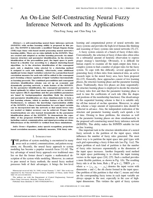
An On-Line Self-Constructing Neural Fuzzy Inference Network and Its ApplicationsChia-Feng Juang and Chin-Teng LinAbstract—A self-constructing neural fuzzy inference network (SONFIN)with on-line learning ability is proposed in this pa-per.The SONFIN is inherently a modiﬁed Takagi–Sugeno–Kang (TSK)-type fuzzy rule-based model possessing neural network’s learning ability.There are no rules initially in the SONFIN.They are created and adapted as on-line learning proceeds via simul-taneous structure and parameter identiﬁcation.In the structure identiﬁcation of the precondition part,the input space is parti-tioned in aﬂexible way according to a aligned clustering-based algorithm.As to the structure identiﬁcation of the consequent part,only a singleton value selected by a clustering method is assigned to each rule initially.Afterwards,some additional signiﬁcant terms(input variables)selected via a projection-based correlation measure for each rule will be added to the consequent part(forming a linear equation of input variables)incrementally as learning proceeds.The combined precondition and consequent structure identiﬁcation scheme can set up an economic and dynamically growing network,a main feature of the SONFIN. In the parameter identiﬁcation,the consequent parameters are tuned optimally by either least mean squares(LMS)or recursive least squares(RLS)algorithms and the precondition parameters are tuned by backpropagation algorithm.Both the structure and parameter identiﬁcation are done simultaneously to form a fast learning scheme,which is another feature of the SONFIN. Furthermore,to enhance the knowledge representation ability of the SONFIN,a linear transformation for each input variable can be incorporated into the network so that much fewer rules are needed or higher accuracy can be achieved.Proper linear transformations are also learned dynamically in the parameter identiﬁcation phase of the SONFIN.To demonstrate the capa-bility of the proposed SONFIN,simulations in different areas including control,communication,and signal processing are done. Effectiveness of the SONFIN is veriﬁed from these simulations. Index Terms—Equalizer,noisy speech recognition,projection-based correlation measure,similarity measure,TSK fuzzy rule.I.I NTRODUCTIONT HE problem of system modeling is encountered in many areas such as control,communications,and pattern recog-nition,etc.Recently,the neural fuzzy approach to system modeling has become a popular research focus[1]–[4].The key advantage of neural fuzzy approach over traditional ones lies on that the former doesn’t require a mathematical de-scription of the system while modeling.Moreover,in contrast to pure neural or fuzzy methods,the neural fuzzy method possesses both of their advantages;it brings the low-levelManuscript received July10,1996;revised January7,1997.This work was supported by the National Science Council,Republic of China,under Grant NSC85-2212-E-009-044.The authors are with the Department of Control Engineering,National Chiao-Tung University,Hsinchu,Taiwan,R.O.C.Publisher Item Identiﬁer S1063-6706(98)00794-2.learning and computational power of neural networks into fuzzy systems and provides the high-level human-like thinking and reasoning of fuzzy systems into neural networks[5]–[7].A fuzzy system consists of a bunch of fuzzy if-then rules. Conventionally,the selection of fuzzy if-then rules often relies on a substantial amount of heuristic observation to express proper strategy’s knowledge.Obviously,it is difﬁcult for human experts to examine all the input–output data from a complex system toﬁnd a number of proper rules for the fuzzy system.To cope with this difﬁculty,several approaches to generating fuzzy if-then rules from numerical data,an active research topic in the neural fuzzy area,have been proposed [6]–[15].Generally,these approaches consist of two learning phases,the structure learning phase and the parameter learning phase.Traditionally,these two phases are done sequentially; the structure learning phase is employed to decide the structure of fuzzy rulesﬁrst and then the parameter learning phase is used to tune the coefﬁcients of each rule(like the shapes and positions of the membership functions).One disadvantage of this sequential learning scheme is that it is suitable only for off-line instead of on-line operation.Moreover,to adopt this scheme a large amount of representative data should be collected in advance.Also,the independent realization of the structure and parameter learning usually each spends a lot of time.Owning to these problems,the structure as well as the parameter learning phases are done simultaneously in the proposed self-constructing neural fuzzy inference network (SONFIN).This ability makes the SONFIN suitable for fast on-line learning.One important task in the structure identiﬁcation of a neural fuzzy network is the partition of the input space,which inﬂuences the number of fuzzy rules generated.The most direct way is to partition the input space into grid types with each grid representing a fuzzy if-then rule[see Fig.1(a)].The major problem of such kind of partition is that the number of fuzzy rules increases exponentially as the dimension of the input space increases.Another frequently used method for input space partitioning is to cluster the input training vectors in the input space[24],[25].Such a method provides a moreﬂexible partition,as shown in Fig.1(b).The resulting fuzzy rule is of the form,Ruleis is(a)(b)(c)(d)Fig.1.Fuzzy partitions of two-dimensional input space.(a)Grid-type par-titioning.(b)Clustering-based partitioning.(c)GA-based partitioning.(d)Proposed aligned clustering-based partitioning.that what a fuzzy rule means and how it works should be easy to understand.We may solve this problem by projecting the generated cluster onto each dimension of the input space to form a projected one-dimensional (1-D)membership function for each input variable and represent a cluster by the product of the projected membership functions,as illustrated in Fig.1(b).Compared with the grid-type partition,the clustering-based partition does reduce the number of generated rules,but not the number of membership functions of each input variable.To verify this,suppose thereareparts(clusters formed,then the number of membership functionsgeneratedis.Ingeneral,,meaning that the clustering-based partition creates more membership functions than the grid-type one dose.In fact,by observing the projected membership functions in Fig.1(b),we ﬁnd that some membership functions projected from different clusters have high similarity degrees.These highly similar membership functions should be eliminated.This phenomenon occurs not only in the clustering-based partitioning methods,but also in other approaches like those based on the orthogonal least square (OLS)method [16],[17].Another ﬂexible input space partitioning method is based on the genetic algorithm (GA)[28],which has the partition result as shown in Fig.1(c).The major disadvantage of this method is that it is very time consuming;the computation cost to evaluate a partition result encoded in each individual is very high and many generations are needed to ﬁnd the ﬁnal partition.Hence,this scheme is obviously not suitable for on-line operation.Moreover,the GA-based partitioning methods might not ﬁnd meaningful fuzzy terms for each input variable,as illustrated in Fig.1(c).In this paper,we develop a novel on-line input space partitioning method,which is an aligned clustering-based approach.This method can produce a parti-tion result like the one shown in Fig.1(d).Basically,it aligns the clusters formed in the input space,so it reduces not only the number of rules but also the number of membership functions under a prespeciﬁed accuracy requirement.The proposed method creates only the signiﬁcant membership functions on the universe of discourse of each input variable by using a fuzzy measure algorithm.It can thus generate necessary fuzzy rules from numerical data dynamically.In [17],the most signiﬁcant rules are selected based upon OLS method.To use this method,the learning data should be collected in advance and the parameters of the fuzzy basis functions are ﬁxed.The generated fuzzy rules by this method are signiﬁcant only for the ﬁxed input–output training pairs collected in advance,so it is not suitable for on-line learning.Since our objective is on-line learning,and the input membership functions are all tunable,a rule is considered to be necessary and is generated when it has a low overlapping degree with others.Another objective of this paper is to provide an optimal way for determining the consequent part of fuzzy if-then rules during the structure learning phase.Different types of consequent parts (e.g.,singletons,bell-shaped membership functions,or a linear combination of input variables)have been used in fuzzy systems [22].It was pointed out by Sugeno and Tanaka [20]that a large number of rules are necessary when representing the behavior of a sophisticated system by the ordi-nary fuzzy model based on Mamdani’s approach.Furthermore,they reported that the Takagi–Sugeno–Kang (TSK)model can represent a complex system in terms of a few rules.However,even though fewer rules are required for the TSK model,the terms used in the consequent part are quite considerable for multi-input/multi-output systems or for the systems with high-dimensional input or output spaces.Hence,we encounter a dilemma between the number of fuzzy rules and the number of consequent terms.A method is proposed in this paper to solve this dilemma,which is,in fact,a combinational optimization problem.A fuzzy rule of the following form is adopted in our system initiallyRuleandTHEN is a fuzzy set,andFig.2.Structure of the proposed SONFIN.employed in conjunction with the precondition identiﬁcation process to reduce both the number of rules and the number of consequent terms.Associated with the structure identiﬁcation scheme is the parameter identiﬁcation scheme used in the SONFIN.In the parameter identiﬁcation scheme,the consequent parameters (coefﬁcients of the linear equations)are tuned by either least mean squares(LMS)or recursive least squares(RLS)algo-rithms and the precondition parameters(membership functions of input variables)are tuned by the backpropagation algorithm to meet the required output accuracy.Furthermore,to enhance the knowledge representation capability of the SONFIN,a linear transformation of the input variables can be incorporated into the network to further reduce the rule number or to achieve higher output accuracy.Proper linear transformation is also tuned automatically during the parameter learning phase.Both the structure and parameter learning are done simultaneously for each incoming training pattern to form a fast on-line learning scheme.This paper is organized as follows.Section II describes the basic structure and functions of the SONFIN.The on-line structure/parameter learning algorithms of the SONFIN is presented in Section III.In Section IV,the SONFIN is applied to solve several problems covering the areas of control, communication,and signal processing.Finally,conclusions are summarized in the last section.II.S TRUCTURE OF THE SONFINIn this section,the structure of the SONFIN(as shown in Fig.2)is introduced.This six-layered network realizes a fuzzy model of the following form:RuleandTHENis a fuzzyset,is the center of a symmetric membership functionon is a consequent parameter. It is noted that unlike the traditional TSK model where all the input variables are used in the output linear equation,only the signiﬁcant ones are used in the SONFIN,i.e.,some,which serves to combine information,activation,or evi-dence from other nodes.This function provides the net inputfor this nodenet-inputare inputs to this nodeandnet-inputdenotes the activation function.We shall nextdescribe the functions of the nodes in each of the six layersof the SONFIN.Layer1:No computation is done in this layer.Each nodein this layer,which corresponds to one input variable,onlytransmits input values to the next layer directly.Thatisandis unity.Layer2:Each node in this layer corresponds to one lin-guistic label(small,large,etc.)of one of the input variablesin Layer 1.In other words,the membership value whichspeciﬁes the degree to which an input value belongs a fuzzyset is calculated in Layer2.There are many choices for thetypes of membership functions for use,such as triangular,trapezoidal,or Gaussian ones.In this paper,a Gaussianmembership function is employed for two reasons.First,afuzzy system with Gaussian membership function has beenshown to be an universal approximator of any nonlinearfunctions on a compact set[16].Second,a multidimensionalGaussian membership function generated during the learningprocess can be decomposed into the product of1-D Gaussianmembership functions easily.With the choice of Gaussianmembership function,the operation performed in this layerisandandth term of the.Unlikeother clustering-based partitioning methods,where each inputvariable has the same number of fuzzy sets,the number offuzzy sets of each input variable is not necessarily identicalin the SONFIN.Layer3:A node in this layer represents one fuzzy logicrule and performs precondition matching of a rule.Here,weuse the following AND operation for each Layer-3nodeand(4)whereandis then unity.Theoutputandin this layer is unity,too.Layer5:This layer is called the consequent layer.Twotypes of nodes are used in this layer and they are denotedas blank and shaded circles in Fig.2,respectively.The nodedenoted by a blank circle(blank node)is the essential noderepresenting a fuzzy set(described by a Gaussian membershipfunction)of the output variable.Only the center of eachGaussian membership function is delivered to the next layerfor the local mean of maximum(LMOM)defuzziﬁcationoperation[23]and the width is used for output clustering only.Different nodes in Layer4may be connected to a same blanknode in Layer5,meaning that the same consequent fuzzy set isspeciﬁed for different rules.The function of the blank nodeisand(6)where,the center of a Gaussian membershipfunction.As to the shaded node,it is generated only whennecessary.Each node in Layer4has its own correspondingshaded node in Layer5.One of the inputs to a shaded node isthe output delivered from Layer4and the other possible inputs(terms)are the input variables from Layer1.The shaded nodefunctionisand(7)where the summation is over the signiﬁcant terms connected tothe shaded node only,and(a)(b)Fig.3.(a)The region covered by the original input membership functions.(b)The covered region after space transformation.Combining these two types of nodes in Layer 5,we obtain the whole function performed by this layeras(8)Layer 6:Each node in this layer corresponds to one output variable.The node integrates all the actions recommended by Layer 5and acts as a defuzziﬁerwithand(10)where.Aftertransformation,the region that the input membership functions cover is shown in Fig.3(b).It is observed that the rotated ellipse covers the input data distribution well and,thus,a single fuzzy rule can associate this region with its proper output region (consequent).With the transformation of input coordinates,the ﬁring strength calculated in Layer 3(i.e.,the function of a Layer-3node)is changedtoand,then in geometricview,theoperationisandisTHENof the originalvariableis now implicated bythe newvariable,then the transformed rules are the same as the original ones.Generally speaking,the ﬂexibility providedbyduring the learning process without repeated training on the input–output patterns when on-line operation is required. There are no rules(i.e.,no nodes in the network except the input–output nodes)in the SONFIN initially.They are created dynamically as learning proceeds upon receiving on-line incoming training data by performing the following learning processes simultaneously:1)input/output space partitioning;2)construction of fuzzy rules;3)optimal consequent structure identiﬁcation;4)parameter identiﬁcation.In the above,learning process1),2),and3)belong to the structure learning phase and4)belongs to the parameter learning phase.The details of these learning processes are described in the rest of this section.A.Input–Output Space PartitioningThe way the input space is partitioned determines the number of rules extracted from training data as well as the number of fuzzy sets on the universal of discourse of each input variable.Geometrically,a rule corresponds to a cluster in the input space,with(12)whereand the center of clusterbe the newly incoming pattern.Find(13)where is the number of existing rules attime(14)into consideration.In[19],the width of each unitis kept at a prespeciﬁed constant value,so the allocation resultis,in fact,the same as that in[18].In the SONFIN,the width istaken into account in the degree measure,so for a cluster withlarger width(meaning a larger region is covered),fewer ruleswill be generated in its vicinity than a cluster with smallerwidth.This is a more reasonable result.Another disadvantageof[18]is that another degree measure(the Euclid distance)isrequired,which increases the computation load.After a rule is generated,the next step is to decomposethe multidimensional membership function formed in(14)and(15)to the corresponding1-D membership function for eachinput variable.For the Gaussian membership function used inthe SONFIN,the task can be easily doneasandandand,respectively.Assume(17)where.So the approximate similaritymeasureisinput variable is as follows.Suppose no rules are existent initially:IFGenerate a new rule withcenterwidthis a prespeciﬁed constant.After decomposition,wehave.,doP ART2.do nothingELSE,,.Do the following fuzzy measure for each input variabledegreeth input variable.IFdegreeTHEN adopt this new membership function,andsetdetermines thenumber of rules generated.For a higher valueofis a scalar similarity criterionwhich is monotonically decreasing such that higher similarity between two fuzzy sets is allowed in the initial stage of learning.For the output space partitioning,the same measure in (13)is used.Since the criterion for the generation of a new output cluster is related to the construction of a rule,we shall describe it together with the rule construction process in learningprocessinto the structure.To construct the transformationmatrix,if we have no a priori knowledge about it,we can simply set the matrix to be an identity one initially for a new generated rule.The identity assignment meansthat the transformed rule is the same as the original one (without transformation)initially and the inﬂuence of the transformation starts when afterward parameter learning is performed.However,if we have a priori knowledge about the transformation matrix,e.g.,from the distribution of the input data as shown in Fig.3,we can incorporate this transformation into the rule initially.B.Construction of Fuzzy RulesAs mentioned in learning process 1),the generation of a new input cluster corresponds to the generation of a new fuzzy rule,with its precondition part constructed by the learning algorithm in process 1).At the same time,we have to decide the consequent part of the generated rule.Suppose a new input cluster is formed after the presentation of the current input–output training pair();then the consequent part is constructed by the following algorithm:IF there are no output clustersdoreplacedbyﬁndIFconnect inputcluster to theexisting outputclusterto the newlygenerated outputcluster.variables are used as the consequent terms of the SONFIN.The signiﬁcant terms will be chosen and added to the network incrementally any time when the parameter learning cannot improve the network output accuracy any more during the on-line learning process.To ﬁnd the signiﬁcant terms used in the consequent part,we shall ﬁrst discuss some strategies that can be used on-line for this purpose before present our own approach.1)Sensitivity Calculation Method [26]:This is a network pruning method based on the estimation of the sensitivity of the global cost function to the elimination of each connection.To use this method,all the input variables are used in the linear equation of the consequent part.After a period of learning,the coefﬁcients of the linear equation are ordered by decreasing sensitivity values so that the least signiﬁcant terms in the linear equation can be efﬁciently pruned by discarding the last terms on the sorted list.One disadvantage of this method is that the correlation between candidate terms is not detected.Hence,after a term is removed the remaining sensitivities are not necessarily valid for the pruned network and the whole sensitivity estimation process should be performed from the beginning again.2)Weight Decay Method [26]:This is also a network pruning method.Like strategy 1,to adopt this method all input variables are used in the linear equation of the consequent part initially.By adding a penalty term to the cost function,the weights of the fewer signiﬁcant terms will decay to zero under backpropagation learning.The disadvantage of this method is that only the backpropagation learning algorithm can be used and,thus,the computation time is quite long for a weight to decay to zero.Besides,the terms with higher weights are not necessarily the most signiﬁcant ones and,thus,this method usually chooses more terms than necessary.3)Competitive Learning:The link weight (coefﬁcient of consequent linearequation)[10].Aftercompetitive learning,the terms with larger weights are kept and those with smaller ones are eliminated.As in strategy 1,no correlation between the inputs is considered,so the result is not optimal.In the choice of the signiﬁcant terms participated in the consequent part,since the dependence betweenthecandidatesand the desiredoutputandas vectors and ﬁnd thecorrelationbetweenand.The correlation between two vectorsis estimated by the cosine value of theirangleare dependent,then ,otherwise if are orthogonalthen .The main idea of the choice scheme is as follows.Suppose we havechosen vectorsfrom,ﬁnd the correlationvalue betweenthe,then choose the maximumone which isthe candidates,and ﬁnallyset(20)If therearecandidatevectors in each rule,not for other rules.This computation process is based upon the local property of a fuzzy rule-based system,so the vectors from other rules usually have less inﬂuence than the vectors in the same rule and are ignored for computational efﬁciency.For on-line learning,to calculate the correlation degree,we have to store all the input/output sequences before these degrees are calculated.To do this,the size of memory required is oforder ,where are the number of rules,input,and output variables,respectively.Hence,the memory requirement is huge forlargeandtheauto correlation of thesequenceandby(21)are initially equalto zero.For normal correlationcomputation,is used,but for computation efﬁciency and for changing environment where the recent calculations dominate,a constant value,say ,can be ing the stored correlation values in (21)and (22),we can compute the correlation values and choose the signiﬁcant ones.Thealgorithm for this computation is described as follows.In thefollowing,candidates,,denotes the terms already selected by the algorithm,and denotes the essential singletonterm for each rule.Projection-Based Correlation Measure AlgorithmFor eachruledoForCompute(24)(27)where.(30)(31)Thenﬁnd(32)The procedure is terminated attheterms are added to the consequent part of the rule.The consequent structure identiﬁcation scheme in the SON-FIN is a kind of node growing method in neural networks.For the node growing method,in general,there is a question of when to perform node growing.The criterion used in the SONFIN is by monitoring the learning curve.When the effect of parameter learning diminished (i.e.,the output error does not decrease over a period of time),then it is the time to apply the above algorithm to add additional terms to the consequent part.Some other methods for selecting signiﬁcant consequent termsare proposed in [2]and [24].In [2],the forward selection ofvariables (FSV)method is proposed.In this method,different combinations of candidate consequent terms (input variables)are chosen for test.Finally,the one resulting in the minimal error is chosen.This method requires repeated tests and is inefﬁcient.In [24],the OLS learning algorithm is used to select the signiﬁcant terms as well as their corresponding coefﬁcients.To use this method,a block of measured data should be prepared and the input space should be partitioned in advance and kept unchanged.This is not suitable for on-line operation.Moreover,to store the input/output sequence,the memory required is oforder(34)where is the desired outputand is the current output.For each training data set,starting at the input nodes,a forward pass is used to compute the activity levels of all the nodes in the network to obtain the currentoutput .Then,starting at the output nodes,a backward pass is used tocompute for all the hidden nodes.Assumingthat,,and(35)]needs to be computed and propagated.The errorsignalis derivedbyLayer5:Using(8)and(37),the update rulefor(40)(41)where the summation is over the number of links from Layer4for the is updatedby(42)where.In addition to the LMS-like algorithm in(42),to improve the learning speed,the RLS learning algorithm[30]can be used instead in Layers5and6(asbelow)is the corresponding parameter vector,andis a large positive constant.To cope with changingenvironment,ingeneral,,we mayreset(46)wherewhere the summation is performed over theconsequents of a rule node;that is,the error of a rule node isthe summation of the errors of its consequents.Layer3:As in Layer4,only the error signal need becomputed in thislayer(48).(50)So,wehave(51)Layer2:Using(3)and(37),the update ruleofif termnode(56)whereif termnodeSo,the update ruleofis(58)If the transformationmatrixwehave(59)where.Then the update rulesforand(61)and(64)(67)(68)If therole.Tomodify(69)Since both the unknown plant and the SONFIN are driven bythe same input,the SONFIN adjusts itself with the goal ofcausing the output of the identiﬁcation model to match thatof the unknown plant.Upon convergence,their input–outputrelationship should match.The plant to be identiﬁed is guidedby the differenceequationand are thethreshold parameters used in the input and output clusteringprocesses,respectively.Atﬁrst,we use the SONFIN withoutperforming fuzzy measure on the membership functions ofeach input variable,so the number of fuzzy sets of each inputvariable is equal to the number of rules.The training patternsare generatedwith.The training isperformed for50000time steps,where the consequent partis tuned by the LMS algorithm.After training,ten inputandﬁve output clusters are generated.Fig.4(a)illustrates the。

fuzzy方法

fuzzy方法（原创版3篇）目录（篇1）1.模糊方法的定义与特点2.模糊方法的应用领域3.模糊方法的优缺点4.模糊方法的发展前景正文（篇1）一、模糊方法的定义与特点模糊方法是一种基于模糊逻辑的数学方法，它以模糊集合为基础，运用模糊推理和模糊运算等手段来处理现实世界中存在的不确定性和模糊性问题。

模糊方法具有以下特点：1.处理不确定性和模糊性：模糊方法可以对具有不确定性和模糊性的问题进行有效的处理，弥补了传统数学方法在此方面的不足。

2.强调实际应用：模糊方法注重实际问题的解决，强调理论联系实际，将数学理论与实际问题相结合。

3.通用性强：模糊方法可以广泛应用于多个学科领域，如经济学、管理学、工程技术等。

二、模糊方法的应用领域模糊方法在多个领域具有广泛的应用，以下是一些典型的应用领域：1.控制工程：模糊控制是利用模糊逻辑对系统的不确定性和非线性进行建模和控制，以实现更优的控制效果。

2.决策分析：模糊评价、模糊综合评价等方法可以用于多因素、多目标的决策分析，提高决策的准确性和科学性。

3.模式识别：模糊模式识别方法可以用于处理现实世界中的不确定性和模糊性问题，提高识别的准确性。

4.人工智能：模糊方法在人工智能领域具有广泛的应用，如模糊推理、模糊神经网络等。

三、模糊方法的优缺点1.优点：（1）可以处理不确定性和模糊性问题，弥补了传统数学方法的不足；（2）强调实际应用，注重理论联系实际；（3）通用性强，可以应用于多个学科领域。

2.缺点：（1）理论体系尚未完善，需要进一步研究和发展；（2）计算复杂度较高，求解问题需要一定的计算资源。

四、模糊方法的发展前景随着科学技术的不断发展，模糊方法在各个领域的应用将更加广泛，其理论体系也将不断完善。

同时，随着计算机技术的发展，计算能力的提升将有助于降低模糊方法的计算复杂度，提高其应用效果。

目录（篇2）1.模糊方法的定义与特点2.模糊方法的应用领域3.模糊方法的优势与局限性正文（篇2）一、模糊方法的定义与特点模糊方法是一种基于模糊集合理论的数学方法，它以模糊集合为基础，运用模糊逻辑和模糊推理等工具，对问题进行定量或定性分析。

求解线性方程组稀疏解的稀疏贪婪随机Kaczmarz算法

大小 k̂ 。②输出 xj。③初始化 S = {1，…，n}，x0 = 0，
j = 0。④当 j ≤ M 时，置 j = j + 1。⑤选择行向量
ai，i ∈
{
1，…，n
}，每一行对应的概率为
‖a‖i
2 2
‖A‖
2 F
。
⑥
( | ) 确定估计的支持集 S，S = supp xj-1 max { k̂，n-j+1 } 。
行从而达到加快算法收敛速度的目的。算法 3 给出
稀疏贪婪随机 Kaczmarz 算法。
算法 3 稀疏贪婪随机 Kaczmarz 算法。①输入
A∈ Rm×n，b ∈ Rm，最大迭代数 M 和估计的支持集的
大小 k̂ 。 ② 输出 xk。 ③ 初始化 S = {1，…，n}，x0 =
x
* 0
=
0。④
置
k
=
0
时，当
k
≤
M
-
1
时。⑤计算
( {| | } ϵk=
1 2
‖b
1 - Ax‖k 22
max
1≤ ik ≤ m
bik - aik xk 2
‖a
‖ ik
2 2
+
)1
‖A‖
2 F
（2）
⑥决定正整数指标集
{ | | } Uk =
ik|
bik - aik xk
2
≥
ϵ‖k b
-
Ax‖k
‖22 a
‖ ik
2 2
ï í
1
ï î
j
l∈S l ∈ Sc
其中，j 为迭代步数。当 j → ∞ 时，wj⊙ai → aiS，因此

fuzzy方法

fuzzy方法（实用版3篇）目录（篇1）1.引言2.介绍模糊方法的基本原理和特点3.模糊方法的应用领域和优势4.模糊方法的优缺点5.结论正文（篇1）一、引言随着科技的不断发展，人工智能技术已经成为当今社会发展的重要趋势。

而在人工智能领域中，模糊方法是一种非常重要的算法。

本文将介绍模糊方法的基本原理和特点，并探讨其在各个领域中的应用。

二、模糊方法的基本原理和特点模糊方法是一种基于模糊数学的理论和方法，其主要特点是能够处理模糊的、不确定的信息。

在模糊方法中，使用了一个称为“隶属函数”的数学工具，用来描述一个对象属于某个集合的程度。

隶属函数可以是线性的或非线性的，可以根据具体问题进行调整。

三、模糊方法的应用领域和优势1.工业制造：在工业制造中，模糊方法可以用来解决复杂的问题，如质量控制、生产调度等。

通过建立数学模型，模糊方法可以自动地优化生产流程，提高生产效率。

2.医疗诊断：在医疗诊断中，模糊方法可以用来处理大量的数据，如医学影像、病理分析等。

通过使用模糊方法，医生可以更加准确地诊断疾病，提高治疗效果。

3.自然语言处理：在自然语言处理中，模糊方法可以用来处理不确定的信息，如语义理解、情感分析等。

通过使用模糊方法，可以提高机器翻译的准确性和情感分析的准确性。

4.交通管理：在交通管理中，模糊方法可以用来预测交通流量、制定交通规划等。

通过使用模糊方法，可以更好地掌握交通状况，提高交通管理水平。

5.其他领域：除了以上领域，模糊方法还可以应用于许多其他领域，如金融、环境科学等。

通过使用模糊方法，可以更好地处理复杂的问题，提高决策的准确性。

四、模糊方法的优缺点1.优点：（1）能够处理模糊的、不确定的信息；（2）可以自动地优化问题；（3）可以提高机器翻译的准确性和情感分析的准确性；（4）可以更好地掌握交通状况，提高交通管理水平。

2.缺点：（1）需要大量的计算资源；（2）可能存在“维数灾”问题；（3）需要具备一定的数学基础；（4）可能存在“过拟合”问题。

fuzzy方法

fuzzy方法【实用版3篇】篇1 目录1.引言2.Fuzzy 方法的定义和原理3.Fuzzy 方法的应用领域4.Fuzzy 方法的优缺点5.结论篇1正文1.引言Fuzzy 方法是一种基于模糊逻辑的数学方法，由波兰数学家 Zadeh 在 1965 年首次提出。

该方法突破了传统数学中绝对精确的描述方式，引入了模糊性的概念，使得数学模型能够更好地描述现实世界中的不确定性和模糊性。

2.Fuzzy 方法的定义和原理Fuzzy 方法是一种基于模糊集合理论的方法，其核心思想是将现实世界中的事物分为模糊集合，通过对这些模糊集合进行运算和推理，从而得到相应的结论。

模糊集合是由隶属度（即元素属于集合的程度）在 0~1 之间的元素组成的集合，它具有不确定性和模糊性。

3.Fuzzy 方法的应用领域Fuzzy 方法自诞生以来，已经在多个领域取得了广泛的应用，如控制论、信息处理、人工智能、管理科学等。

以下是一些典型的应用领域：（1）控制论：Fuzzy 方法可以用于设计模糊控制器，以解决不确定系统的控制问题。

（2）信息处理：Fuzzy 方法可以用于模糊推理、模糊评价和模糊决策等任务。

（3）人工智能：Fuzzy 方法可以用于构建模糊神经网络、模糊专家系统和模糊知识表示等。

（4）管理科学：Fuzzy 方法可以用于进行模糊预测、模糊优化和模糊评价等。

4.Fuzzy 方法的优缺点Fuzzy 方法的优点主要表现在以下几个方面：（1）能够处理不确定性和模糊性：Fuzzy 方法能够较好地处现实世界中存在的不确定性和模糊性问题。

（2）实用性强：Fuzzy 方法已经在多个领域取得了实际应用，具有较强的实用性。

（3）易于理解和实现：Fuzzy 方法基于模糊集合理论，相对容易理解和实现。

然而，Fuzzy 方法也存在一些缺点，如：（1）理论体系不完善：Fuzzy 方法的理论体系相对不完善，尚需要进一步的研究和完善。

（2）结果的可解释性差：Fuzzy 方法得出的结论往往具有一定的模糊性，可解释性较差。

FuzzyLogicandFuzzyAlgorithms：模糊逻辑和模糊算法

Fuzzy Logic and FuzzyAlgorithmsCISC871/491Md Anwarul Azim(10036952)Presentation OutlineFuzzy control systemFuzzy Traffic controllerModeling and SimulationHardware DesignConclusion2Figure from Prof. Emil M. Petriu, University of Ottawa6Basic Structure of ControllerDEFUZZIFIER –It extracts a crisp value from a fuzzy set.·Smallest of Maximum.·Largest of Maximum.·Centroid of area.·Bisector of Area·Mean of maximum.FUZZIFIERFuzzifier takes the crisp inputs to a fuzzy controller and converts them into fuzzy inputs.FUZZY RULE BASE (Knowledge base)It consists of fuzzy IF-THEN rules that form the heart of a fuzzy inference system. A fuzzy rule base is comprised of canonical fuzzy IF-THEN rules of the form IF x1 is A1(l) and ... and xn is An (l)THEN y is B(l), where l = 1, 2, ...,M. Should have Completeness, Consistency, Continuity..FUZZY INFERENCE ENGINEFuzzy Inference Engine makes use of fuzzy logic principles to combine the fuzzy IF-THEN rules. Composition based inference (Max/Min,Max/Product)and individual-rule based inference (Mamdani). Other methods like Tsukamoto, Takagi Sugeno Kang (TSK)7“Fuzzy Control”Kevin M. Passino and Stephen Yurkovichhttp://if.kaist.ac.kr/lecture/cs670/textbook/ Fuzzy Traffic controller--Most traffic has fixed cycle controllers that need manual changes to --One of the desirable features of traffic controllers is to dynamically effect the change of signal phase durations--This problem can be solved by use of fuzzy traffic controllers whichadaptively at an intersection.12 /help/toolbox/fuzzy/fp243dup9.html13 /watch?v=hFWGToL-NHw/products/simulink/demos.htmlModeling using Simulink(Cont.)14 /watch?v=hFWGToL-NHw/products/simulink/demos.html15Case Study 2 (Extra)17。

外文翻译原文

An Optimal Fuzzy-PI Controller for the High-PerformanceSpeed Control of a PMSMAbstract—The purpose of this paper is to present an adaptive method for improving the control performance of permanent magnetic synchronous motor (PMSM) in operating condition. The approach allows to reduce speed tracking error and to cope with external disturbance. The methodology of speed control is presented in detail and two controllers are tested, traditional proportional integrative (PI) controller and fuzzy proportional integrative (fuzzy-PI) controller. Both controllers showed good results from experiments presenting similar behaviors. However, the fuzzy-PI stood out positively in some stages. The main motivation of this paper is the extension of fuzzy logic algorithm to improve servo control performance in industrial applications.Keywords-Fuzzy-PI; Speed Control; Disturbance; PMSMIntroductionHigh-performance servo system for permanent magnetic synchronous motor (PMSM) is essential in many applications in the field of mechatronics such as precision engineering, computer numerically controlled machine tools and other applications in a variety of automated industrial plants . Due to the uncertainties, which are composed of unpredictable plant parameter variations, load disturbances, and nonlinear dynamics of the plant , the control performance of PMSM servo system is influenced seriously. In this situation, the servo drive may need to respond relatively swiftly to command changes and to offer enough robustness against the uncertainties. In order to meet the development requirements of high speed and high precision for linear motor, it is thus desired to have an intelligent controller that can own higher anti-disturbance performance according to the disturbances and uncertainties in operating condition.Up to now, a large number of control techniques (fuzzy, PI, PID, etc.) with varying complexity have been proposed . Fuzzy control was first introduced and implemented in the early 1970 in an attempt to design controllers for systems that are structurally difficult to model due to naturally existing nonlinearities and other modeling complexities. Sant et al. present the vector control of PMSM with hybrid fuzzy PI speed controller with switching functions calculated based on the weights. Yen-Shin Lai et al. present a new hybrid PI-type fuzzy controller for direct torque control induction motor drives with fast tracking capability, less steady state error, and robust to load disturbance. In summary, fuzzy logic control appears very useful when the processes are too complex to analyze by conventional quantitative techniques. It seems clear to everyone that speed control techniques have allowed to execute increasingly more complex tasks in servo system field.The performance of the fuzzy-PI controllers also depends on the choice of a suitable optimization algorithm. In this paper, an adaptive speed controller is proposed to minimize oreliminate the speed tracking error. The designed hybrid fuzzy-PI controller improves system performance in the transient and steady state. This paper is organized as follows. In section 2, the vector control and disturbance effects for PMSM are described in detail. The adaptive fuzzy-PI controller is explained in section 3, whilst experimental results are presented in section 4 and conclusions are drawn in the final section.Pmsm vector controlIn the PMSM, excitation flux is set-up by magnets; subsequently magnetizing current is not needed from the supply . This easily enables the application of the flux orientation mechanism by forcing the magnetizing current component of the stator current vector to be zero. As a result, the electromagnetic torque will be directly proportional to the torque current component of the stator current vector, hence better dynamic performance is obtained by controlling the electromagnetic torque separately. A system configuration of a vector control PMSM servo system is shown in Fig. 1. In the vector control scheme, torque control can be carried out by suitable regulation of the stator current vector; this implies that accurate speed control depends on the regulated current vector.qr Figure 1. The system configuration of a vector control PMSMSpeed control system of PMSM is also multi-variable, nonlinear, strong-coupled system, and the disturbances mainly include the load inertia and load torque. In the running of servo system, system inertia may change. When the system inertia increases, the response of servo system will slow down, which is likely to cause system instability and result in climb. On the contrary, when the system inertia decreases, dynamic response will speed up with speed overshoot as well as turbulence. Meanwhile, the main role of servo system is to drive the load operation, but in many industries, the load carried by servo system is not constant. Changes in the load torque will have significant impact on servo control performance: in the running of servo system, the sudden increase or reduce of load torque would result in fluctuations in servo speed control, affecting the accuracy of positioning and control performance.Design of speed controllerIn this paper, we are proposing a speed control scheme based on fuzzy logic to improve the control performance for PMSM. Speed controller can be implemented using several approaches, such as PI, fuzzy, etc. However, when implementing a speed controller the following conditions should be considered:z Simplicity: The speed control law must be simple and easy to compute in order toenable fast servo adaptation.z PI-type control: In order to achieve a null steady state error, a PI type speed control lawshould be selected and implemented.z Implementation requirements should not include significant changes to the original control system.Given our objective and system requirements, two control algorithms, PI and fuzzy logic, are chosen. The choice for PI controller is due to its good performance when applied in practical situations, and the preference for fuzzy controller is due to no requirement of the rigorous mathematical system model.Fuzzy Control ArchitectureFuzzy logic was conceived to apply a more human-like way of thinking in computer programming. It is ideal for controlling nonlinear systems and model complex systems where ambiguity is common. It is also potentially very robust, maintaining good closed-loop system performance over a wide range of operating conditions. In our system, speed controller input variables are the speed error e and change of the speed error de :)()()(k k k e f r ωω−= (1))1()()(−−=k e k e k de (2)Where r ω is the speed command and f ω is the actual speed.Fuzzy-PIFrom the conventional PI control algorithm, we can obtain the following discrete equations:)()()(1k i k i k i q q q Δ+=− (3))()()(k e k k de k k i i p q +=Δ (4)If e and de are fuzzy variables, (3) and (4) become a fuzzy control algorithm. Then, the centre of area method is selected for defuzzify the output fuzzy set inferred by the controller:∑∑==Δ=Δn i ini q i q i i i 11)(ηη (5) Where i η is the membership function, which takes values in the interval [0, 1].Knowledge BaseThe knowledge base of fuzzy logic controller is composed of two components, namely, a database and a fuzzy control rule base. The well-known PI-like fuzzy rule base is used in this paper (Table 1). The surface of rule base is shown in Fig. 2. It allows fast working convergence without significant oscillations and prevents overshoots and undershoots.TABLE 1 FUZZY RULE BASENM nl nl nm nm ns ze psNS nm nm nm ns ze ps psNZ nm nm ns ze ps ps pmPZ nm ns ns ze ps pm pmPS ns ns ze ps pm pm pmPM ns ze ps pm pm pl plPL ze ps pm pl pl pl plFigure 2. The surface of rule baseTuning StrategyFuzzy logic design is involved with two important stages: knowledge base design and tuning. However, at present there is no systematic procedure to do that. The control rules are normally extracted from practical experience, which may make the result focused in a specific application. The objective of tuning is to select the proper combination of all control parameters so that the resulting closed-loop response best meets the desired design criteria.In order to adapt servo system to different disturbances, the scaling factors should be tuned. The controller should also be adjusted with characteristics representing the scenario to be controlled. These adjustments can be made through the scaling factors, usually applied in any PI controller. S.T. Lin et al. [10] proposed an adjustment where the scaling factors are dynamic and thus they have been adjusted along the task. In this paper, the scaling factors are set to appropriate constant values, achieved by the method of trial and error.ExperimentThe apparatus for the experiment contains three major parts and some data transferring buses, as shown in Fig. 3. These three major parts are: 1) a PC and a PCI with sampling time equal to 1ms; 2) AC servo drive using a DSP plus a FPGA, where DSP TMS320F2812 mainly accomplishes position, velocity and torque control, and FPGA EP2C8Q208C8N is responsible for the analysis and realization of absolute ruler and NCUC-Bus protocols; 3) PMSM with the parameters described in Table 2. Through the PCI controller, PC sends the speed commandand control parameters to servo drive, and receives expected torque current and feedback velocity from servo drive for the model identification.Figure 3. The apparatus for the experimentTABLE2MOTOR PARAMETERSMotor RatingTorque coefficient0.75Nm/ARated speed1000r/minRated Torque4.5NmFriction coefficient0.0008Nms/radInertia0.0028Nms2/radPoles3In the experimental tests without applied load torque, a trapezium-type speed command, the maximum speed of which is 1000r/min, is applied. To evaluate the control performance, a fixed PI controller is considered. Fig. 4 shows the speed response with PI controller, it indicates that the maximum speed error is about 34r/min at the acceleration stage and the maximum speed error fluctuation is about 7r/min at the constant speed stage. Speed response with fuzzy-PI controller is shown in Fig. 5, it has better speed tracking performance with the maximum speed error is about 15r/min at the acceleration stage and the maximum speed error fluctuations is about 3r/min at the constant speed stage.In the experimental tests without applied load torque, a trapezium-type speed command, the maximum speed of which is 1000r/min, is applied. To evaluate the control performance, a fixed PI controller is considered. Fig. 4 shows the speed response with PI controller, it indicates that the maximum speed error is about 34r/min at the acceleration stage and the maximum speed error fluctuation is about 7r/min at the constant speed stage. Speed response with fuzzy-PI controller is shown in Fig. 5, it has better speed tracking performance with themaximum speed error is about 15r/min at the acceleration stage and the maximum speed error fluctuations is about 3r/min at the constant speed stage.Time (s)S p e e d R e s p o n s e (r /m i n)Time (s)S p e e d e r r o r (r /m i n )Figure 4. The speed response with PI controller (no load torque)Time (s)S p e e d R e s p o n s e (r /m i n)Time (s)S p e e d e r r o r (r /m i n )Figure 5. The speed response with fuzzy-PI controller (no load torque)In the experimental tests with changed applied load torque, a slope-type speed command, the maximum speed of which is 1000r/min, is applied. When s t 2=, the applied load torque is 2Nm. When s t 5=, the applied load torque is suddenly became to 8Nm. To evaluate the control performance, a fixed PI controller is also considered. Fig. 6 shows the speed response with PI controller. When s t s 52<≤, the maximum speed error is about 95r/min at the acceleration stage and marked speed overshoot at the constant speed stage. When s t s 105<≤, it is clear that the maximum speed error fluctuation is about 50r/min and the tracking response does not meet the design specifications.Speed response with fuzzy-PI controller is shown in Fig. 7. When s t s 52<≤, the maximum speed error is only about 48r/min at the acceleration stage and unobvious speed overshoot at the constant speed stage. When s t s 105<≤, it is clear that the maximum speederror fluctuations is only about 8r/min. servo system with fuzzy-PI controller has better speed tracking performance and can suppress the load torque well.Time (s)S p e e d R e s p o n s e (r /m i n )Time (s)S p e e d E r r o r (r /m i n )Figure 6. The speed response with PI controllerTime (s)S p e e d R e s p o n s e (r /m i n )Time (s)S p e e d E r r o r (r /m i n )Figure 7. The speed response with fuzzy-PI controllerConclusionsThis paper has presented an adaptive fuzzy-PI speed control scheme for PMSM drive. The effectiveness of the proposed approach was proved through experiments, showing that the hybrid control improves significantly servo performance, making servo system more human-like, flexible and with capacity to make decisions. Substantially, the fuzzy-PI controller can occur a small overshoot against a large overshoot when using the PI controller. Furthermore, in some situations the fuzzy-PI controller showed to be a better solution to reach the set-point faster.。

基于新的松弛条件的离散时间2-D T-S模糊系统的镇定

更多技术文章，论文请登录
Vol. 36, No.ቤተ መጻሕፍቲ ባይዱ2
ACTA AUTOMATICA SINICA
February, 2010
Stabilization of Discrete-time 2-D T-S Fuzzy Systems Based on New Relaxed Conditions
Manuscript received October 6, 2008; accepted March 5, 2009 Supported by National Natural Science Foundation of China (50977008, 60904017, 60774048, 60728307), the Funds for Creative Research Groups of China (60521003), the Program for Cheung Kong Scholars and Innovative Research Team in University (IRT0421), and the 111 Project (B08015), National High Technology Research and Development Program of China (863 Program) (2006AA04Z183) 1. Key Laboratory of Integrated Automation for the Process Industry, Ministry of Education, Shenyang 110004, P. R. China 2. School of Information Science and Engineering, Northeastern University, Shenyang 110004, P. R. China

Fuzzy Logic

Causal Probabilistic Networks or Bayesian Networks Probability calculus is a well-established tool for handling uncertainty with a history of about 300 years. Today, Bayesian networks or Causal Probabilistic Networks CPN represent a culmination of Bayesian probability theory and causal graphical representations for modeling causal and probabilistic applications. There are two essential problems harassing proponents and adherents of Bayesian networks or probabilists in general. The rst is a theoretical problem. Probability calculus is based on an axiomatic de nition which in turn is based on the classical bivalent logic. This logic as the basis for the precision of mathematics is attributed to Aristotle's Laws of Thought". In particular, one of these laws, called the Law of the Excluded Middle" claims that every proposition must be

基于词计算的Fuzzy有限自动机的最小化

基于词计算的Fuzzy有限自动机的最小化
张诗静;舒兰
【期刊名称】《西南科技大学学报》
【年(卷),期】2009(24)1
【摘要】介绍了一种基于词计算的一类新的Fuzzy有限自动机,这种自动机的输入和输出分别由输入和输出字母表的Fuzzy子集串代替,定义了它的最小形式,得到这种新的Fuzzy有限自动机M都存在一个与之等价的最小Fuzzy有限自动机Mm.【总页数】4页(P82-84,90)
【作者】张诗静;舒兰
【作者单位】西南科技大学理学院,四川绵阳,621010;电子科技大学应用数学学院,四川成都,610054
【正文语种】中文
【中图分类】TP301.1
【相关文献】
1.基于词计算的Fuzzy有限自动机的等价问题 [J], 张诗静
2.基于粗糙集理论的有限自动机最小化方法改进 [J], 李科;杨瑞敏
3.基于信息系统的确定有限自动机最小化算法 [J], 杨传健;葛浩;姚光顺;王波
4.融合区块链与边缘计算系统中基于最小化网络时延的TOSML优化方案 [J], 李聪;刘通
5.基于模糊字符串的Mealy格值有限自动机及其最小化 [J], 汪洋;莫智文
因版权原因，仅展示原文概要，查看原文内容请购买。

fuzzy estimation method

文章标题：深度剖析模糊估计方法1. 引言在现代科学和工程领域中，面对复杂系统和模糊问题的时候，我们常常需要借助于模糊估计方法来处理。

模糊估计方法是一种能够处理不确定性和模糊性的数学工具，其在决策分析、控制系统、模式识别等领域有着广泛的应用。

2. 模糊估计方法的基本原理模糊估计方法是基于模糊集理论的，模糊集是一种能够描述不确定性和模糊性的数学工具。

在模糊估计方法中，我们首先需要对问题领域进行模糊化，然后利用模糊集的运算规则进行模糊推理，最终得到模糊的估计结果。

模糊估计方法的基本原理是将模糊集的概念应用于估计过程，以应对现实世界中的模糊和不确定性。

3. 模糊估计方法的应用领域模糊估计方法在实际应用中有着广泛的应用，例如在工程领域中，我们可以利用模糊估计方法来处理复杂系统的控制问题；在经济领域中，模糊估计方法可以用来进行风险评估和投资决策；在医学领域中，模糊估计方法可以用来处理疾病诊断和治疗方案设计等。

4. 模糊估计方法的优缺点模糊估计方法的优点在于能够处理不确定性和模糊性，对于复杂系统和问题有着良好的适用性；但其缺点在于需要准确地建立模糊集的隶属函数和运算规则，且在实际应用中需要大量的专业知识和经验。

5. 个人观点和总结作为一种处理模糊问题的数学工具，模糊估计方法在现实世界中有着重要的应用意义。

但在实际应用中，我们需要充分了解问题的领域特点，结合专业知识和经验来准确地建立模糊集和运算规则，以获得可靠的估计结果。

随着人工智能和大数据技术的发展，模糊估计方法也在不断得到改进和拓展，将为解决更多复杂问题提供更加有效的数学工具。

以上是我对模糊估计方法的个人理解和观点，希望能够对您有所帮助。

6. 模糊估计方法的发展历程模糊估计方法作为一种处理模糊和不确定性问题的数学工具，其发展历程可以追溯至上世纪50年代。

最早提出模糊集的概念是由日本学者石川明于1965年提出的，其将不确定性因素引入了数学模型中。

随后，模糊估计方法被广泛应用于控制理论、人工智能、决策分析等领域，且在不断得到改进和拓展的过程中，逐渐成为一种重要的工程工具。

建立经济分析模型的Fuzzy方法与应用

生活一点通　用木耳浸泡在盐水里大约一小时左右,再用冷水洗涮几次,可洗除沙子。

建立经济分析模型的Fuzzy 方法与应用◆中央财经大学教授　吴秉坚一、问题的提出利用经济计量模型对某一经济变量进行定量分析的主要步骤是:将待研究的经济变量作为被解释变量,在定性分析的基础上找出影响该变量的主要因素作为解释变量,将其它次要因素的总和作为随机扰动项;然后通过回归分析建立反映解释变量与被解释变量之间相关性的数学方程;当模型经过经济检验和统计检验达到要求的可靠程度时,就可以用模型对待研究的经济变量作结构分析与趋势预测。

但是回归分析的前提是假定除解释变量外影响被解释变量的因素都是一些偶然的随机性因素,然而实际经济活动中除随机性因素外还存在着具有边界不分明特征的模糊性因素。

如果模糊性因素的作用较大时,必然会使经济计量模型受到影响。

本文讨论用模糊系统分析的方法建立反映经济变量之间相关性的数学模型,当经济变量之间的相关性受到未知的模糊性因素影响时,本文的方法可以在一定程度上改进经济计量模型的不足。

模糊系统分析是在美国信息论专家L.A.Zadeh 教授1965年首先提出的Fuzzy 集合的基础上发展起来的一门新兴的科学分支。

近年来模糊系统分析中的聚类分析、综合评价、模糊规划等方法已经在经济问题的研究中得到了很好的应用,然而直接利用F uzzy 集合的方法建立反映经济变量之间相关性的数学方程的研究还不多见,本文也仅仅是利用F uzzy 集合的方法建立经济分析模型的初步尝试。

二、数学模型的建立首先,设在某个问题的研究中被解释变量为y ,解释变量为X 1,X 2……,X k 。

当解释变量取一组定值时,假设被解释变量是依赖于解释变量而确定的一个模糊数Y 。

因此设理论上的数学模型为Y=A 1X 1+A 2X 2+……+A K X K其中解释变量X j 的系数A j (j=1,2……K )是一个以a j 为中心值,以C j 为模糊半径的三角模糊数,即A j 的隶属函数为μA j (z )=　1-z -a j C j , a j -C j ≤z ≤a j +C j 0 , 其它,各由Fuzzy 集合论中模糊数的运算性质可知,此时Y 也是一个三角模糊数,并且其中心值a 与模糊半径c分别为a=∑Kj =1a j X j ,　c =∑K j=1c jX j即Y 的隶属函数为μY (z )=　1-z-a C , a -c ≤z ≤a +c 0 , 其它注意到如上模型中A 1,A 2,……A K 是未知模糊数,而A 1,A 2,……A K 一但被确定则被解释变量Y 就可唯一确定。

成为志愿者的理由提升英语能力英语作文

成为志愿者的理由提升英语能力英语作文Reasons Why Volunteering Can Boost Your EnglishHi there! My name is Emma, and I'm 10 years old. I love reading, playing sports, and spending time with my friends and family. One of my biggest goals is to improve my English skills so I can communicate better with people from all around the world. That's why I recently decided to start volunteering at a local community center that helps newcomers to our town learn English. Let me tell you all about the awesome reasons why volunteering has been helping me boost my English abilities!The biggest way volunteering improves my English is through constant practice. At the community center, I get to spend a few hours every weekend conversing with people who are learning English as a second language. By engaging in natural conversations on all sorts of everyday topics, I'm constantly practicing my speaking and listening comprehension skills in a real-world environment. The more I use my English through these interactions, the more comfortable and fluent I become at communicating my thoughts and understanding others.Volunteering has also exposed me to people from many different cultural backgrounds who speak various forms of English. Some have accents that are quite different from the English I'm used to hearing at school and at home. By being immersed in these diverse forms of spoken English, I've become much better at understanding different accents and adapting my own speech to be more universally comprehensible. My ears and brain are getting a great workout when it comes to processing English in all its wonderful variety!The neat thing is, as my conversational English gets stronger through volunteering, my skills in other areas like reading and writing also improve. For example, when explaining instructions or concepts to my English learner friends, I have to be very clear and precise with my word choices and sentence structures. This has made me a better writer and communicator overall. Plus, my enriched vocabulary from learning new words during our chats helps me to understand texts and reading materials at a deeper level.Another way volunteering boosts my English is by allowing me to teach what I know. I've always found that the best way to reinforce my own knowledge is by explaining it to someone else. Whenever I show my English learner friends how to pronounce atricky word or go over the finer points of English grammar, it locks those skills into my brain even more firmly. The process of simplifying complex concepts so a language learner can understand actually demonstrates how well I've mastered that knowledge myself.Volunteering has also exposed me to all sorts of new vocabulary and idiomatic expressions that I hadn't heard before. My English learner friends often ask about colorful slang words or puzzling idioms and phrases. By discussing the nuances of these linguistic concepts with them, I'm constantly expanding my own mastery of the quirky side of English. I can then start sprinkling these more advanced terms and expressions into my own speech and writing.What's really amazing is how energizing it feels to watch my English learner friends' skills steadily improve through our interactions. Seeing their excitement and pride when they grasp a new grammar rule or speak a whole sentence without stumbling fills me with a sense of accomplishment too. It motivates me to be an even better English speaker and model for them. Their success encourages me to keep leveling up my own English abilities.Beyond all the concrete language practice, volunteering is a fun social experience that keeps me excited about constantly working on my English. The community center has a lively, upbeat atmosphere as we all learn together through engaging activities like reading kid-friendly books, acting out skits, or playing vocabulary games. It's an immensely enjoyable way to spend my free time while simultaneously giving back to others. I get that warm, fuzzy feeling of helping others achieve their goals.Volunteering has also allowed me to make lots of new friends from diverse backgrounds that I may not have met otherwise. We can learn so much about different cultures, customs, and perspectives through our conversations. I feel like I'm getting a mini tour around the world without even leaving my hometown! Making these connections inspires me to be an even better communicator so I can clearly express my thoughts while being respectful of all our unique backgrounds.So those are the biggest reasons why I'm so glad I made the choice to become an English conversation volunteer. It's been an incredibly rewarding experience that lets me make a positive impact on others while constantly challenging myself to enhance my English abilities. My vocabulary is more extensive, myconversational fluency has skyrocketed, and my overall reading and writing skills have sharpened tremendously. Most importantly, volunteering has opened my eyes to the rich diversity of cultures and people around the globe — something I hope to explore further as a highly proficient English speaker.If you're looking for an enjoyable way to boost your own English while helping others achieve their dreams, I can't recommend volunteering enough. Get out there and start practicing your English in the real world today! You'll have a world of fun while becoming a true master of the English language.。

无穷论域上的Fuzzy相似选择

无穷论域上的Fuzzy相似选择
王学顺;谢冬梅
【期刊名称】《东北林业大学学报》
【年(卷),期】1996(024)004
【摘要】在已有的Ｆｕｚｚｙ相似选择问题中，许多都是在有限论域上讨论的。

本文讨论了无穷论域上的Ｆｕｚｚｙ相似选择问题，使Ｆｕｚｚｙ相似选择趋于完全化、通过给出无穷论域上的相似优先比的定义，并对其进行集值统计估值，从而给出了Ｆｕｚｚｙ相似选择的新方法。

这个方法对于有限论域上的相似选择也适用，最后给出了进行Ｆｕｚｚｙ相似选择的新准则，并证明了利用准则进行相似选择与原准则有相同的效果。

【总页数】3页(P117-119)
【作者】王学顺;谢冬梅
【作者单位】不详;不详
【正文语种】中文
【中图分类】O159
【相关文献】
1.L—Fuzzy集上的Fuzzy数值Fuzzy测度和Fuzzy数值Fuzzy积分 [J], 张广全
2.Fuzzy模式识别方法和Fuzzy相似选择方法在班级管理中的应用 [J], 陈茵
3.有限论域上Fuzzy事件的概率 [J], 闫家杰
4.连续论域上Fuzzy集的信息熵 [J], 仇计清;姜文鹏;周长杰
5.论域无限时完备完全分配格上■-Fuzzy关系方程解集的一些性质和结构 [J], 王赟;王学平;屈小兵
因版权原因，仅展示原文概要，查看原文内容请购买。

Fuzzy的产品概念设计的形式化方法的研究的开题报告

集成TOC/TRIZ/Fuzzy的产品概念设计的形式化方法的研究的开题报告一、选题背景目前，在众多产品设计过程中，面对创新设计、技术开发等问题，设计师和工程师们通常采用各种方法，如创意法、设计思维、用户需求分析等等，以期望从中获得优秀的产品概念设计方案。

其中，TOC （Theory of Constraints）、TRIZ（Theory of Inventive Problem Solving）和Fuzzy（模糊集合）作为工程设计领域中常用的分析工具，可以分别用于解决设计中的约束、难题和不确定性问题。

然而，由于现有方法的局限性，一些问题仍未解决，在实际产品设计过程中提高创新力、降低设计风险、提高产品质量等继续是重要挑战。

由此，本研究选择以集成TOC、TRIZ、Fuzzy三个方法为核心的，形式化方法的产品概念设计的研究为开题研究方向，旨在为解决现有方法的不足提供更全面、更有效的设计思路和工具。

二、研究目的本研究的目的在于，研究并提出一种集成TOC、TRIZ、Fuzzy的产品概念设计形式化方法，主要实现以下几个方面：1. 为设计师和工程师提供一种综合性的产品概念设计方法；2. 提高产品概念设计的创新性，以更好地满足用户需求；3. 减少因设计决策不确定性而导致的风险；4. 提高产品设计质量和竞争力。

三、研究内容本研究拟采用以下几个步骤：1. 初步调研：分析现有TOC、TRIZ、Fuzzy方法中的优缺点，并研究其中能够集成的部分；2. 概念设计框架设计：通过框架化设计，将三个方法集成于一体，形成一个适用于概念设计的框架。

在框架设计过程中，必须考虑到三个方法的应用目的、原理和适用范围，并在集成过程中解决彼此之间的冲突和问题；3. 案例研究：通过案例研究，验证集成的产品概念设计方法的有效性和实际应用性；4. 结果分析：对经过验证的方法进行总结和分析，界定方法的适用范围，以期望达到创新设计、降低设计风险、提高产品质量等目标。

运用FUZZY数学方法对学生教学能力进行综合评定的初步研究

运用FUZZY数学方法对学生教学能力进行综合评定的初步研
究
龚德贵
【期刊名称】《常德师专学报：自然科学版》
【年(卷),期】1989(010)002
【总页数】10页(P56-64,92)
【作者】龚德贵
【作者单位】无
【正文语种】中文
【中图分类】O1－42
【相关文献】
1.综合运用层次分析法和模糊数学方法对我国研究生培养模式进行评价 [J], 陈少雄
2.运用模糊数学方法对田径运动技术进行综合评定的研究 [J], 汪鸿
3.运用模糊数学方法对排球运动技术进行综合评定的研究 [J], 黄延春
4.在体育科研中运用Fuzzy(模糊)数学方法进行配对实验设计的初步探讨 [J], 吕强
5.运用fuzzy(模糊)数学方法对教学水平进行综合评判的初步探讨 [J], 吕强
因版权原因，仅展示原文概要，查看原文内容请购买。

1、下载文档前请自行甄别文档内容的完整性，平台不提供额外的编辑、内容补充、找答案等附加服务。
2、"仅部分预览"的文档,不可在线预览部分如存在完整性等问题,可反馈申请退款(可完整预览的文档不适用该条件!)。
3、如文档侵犯您的权益，请联系客服反馈,我们会尽快为您处理(人工客服工作时间：9:00-18:30)。

Given a set L = {xan affirmed or a negated propositional variable of a Boolean formula, we denote by X n={0,1}n the space of the Boolean vectors x of size n , that can be assigned to the literals of L. We denote by C the class of such formulas, called concepts elsewhere, and, for gŒC, by set(g ) the set of all the literals occurring in the formula g . A formula is monotone if only affirmed variables appear in it. Given a set M = {m 1, …, mm} of m monomials, built as a conjunction of literals in L, a formula g=»i mi is a DNF. By abuse, we will use the same notation for g and support(g), i.e. the set of points xŒXn such that g ( x)=1. For a given concept g, E+Ã Xn and E-Ã X n are the sets of positive and negative examples respectively, constituted by assignments belonging the former and not belonging the latter to g.
U
Given a set of examples E , we simply compute a minimal DNF crisp monotone description through the algorithm of Table 1. Table 1.Construction of aDNF from examples. Construction (E+, E-) BEGIN DNF = ∅ FOR_ALL uŒE+ m = «i |ui = 1 xi DNF = DNF »{m} Return DNF END It is easy to check that m is the smallest monotone monomial containing the positive sampled point on whose basis it has been created. 3. SYMPLIFYING AN INFERRED DNF
Definition 2.1: Let us represent a monomial m by the vector m = (b 1, …, b n) where bi = 1 if xiŒm and bi = 0 otherwise; each binary value bi is the crisp membership value of xi to m . With a similar notation, we represent a k k -term_DNF g = m i by a vector B of length nk i =1 obtained by concatenating the representations of the joined monomials. We say that g =»i mi is a DNF crisp description of E= E+ » E- if g is consistent with all the positive and negative points of E.
The jump from examples to concepts, for instance from fire observations to the settlement of the thermodynamics laws, might be very long, taking a complex sequence of hierarchical steps, like human kind did over the course of the centuries. In view of capturing some features of this abstraction process, we raised up an agnostic learning procedure [1] that generates a minimal function consistent with the examples, in the sense that no formula whose support is included in this function can maintain the consistency. In turn, consistency means that, once we have a set of examples labeled by a flag telling us whether the example must belong to the final formula (positive example) or not (negative one), the formula we find must respect the flags. This kind of minimality however does not guarantee an analogous minimality on the formula description length [2]. Thus, we propose here an algorithm to reduce the number of literals in the formula still preserving its descriptional power. A shortening may happen for free, when for instance we discover a new monomial still consistent with the examples and including two smaller ones belonging to the formula. However, we accept to sacrifice some accuracy of the formula to get it shorter. It is the typical attitude with which we interpolate a set of experimental
FUZZY METHODS FOR SIMPLIFYING A BOOLEAN FORMULA INFERRED FROM EXAMPLES
B. Apolloni, D. Malchiodi, C. Orovas, A. M. Zanaboni Dipartimento di Scienze dell’Informazione – Università degli Studi di Milano-ITALY ABSTRACT In order to state a symbolic description of observed data we learn a minimal monotone DNF (Disjunctive Normal Form) formula consistent with them. Then, in the idea that a short formula – i.e. made up of few monomials, each represented by the product of few literals – is better understandable by the user than a longer one, we propose here an algorithm to simplify in this direction the formula learnt from examples. We obtain concise formulas by violating their consistency on a part of the observed examples in some regions of the sample space that we consider as fuzzy borders of the formulas. Special membership functions to these regions allow us to manage the balance between conciseness and description power of the final formula as an optimisation problem that is solved via a simulated annealing procedure on a set of artificially constructed benchmarks. 1. INTRODUCTION points with a line: we don’t assume that a true linear relation exists between the point coordinates, but such relation helps us to understand the bulk of the phenomena underlying the points. In our case we may see a consistency violation of the concise formula either as a consequence of a fuzzy definition [3] of its support’s contour or as denoting a non clear classification of the missed point flags. Here we prefer the first perspective and use a special membership function to the fuzzy support of the formula to characterize a thickness of the fuzzy border. This allows us to translate the above problem of balancing complexity versus approximation of the final formula into the analogous balancing of its descriptional length and the mean thickness of the borders of the constituting monomials. We tested numerically the suitability of this perspective on a set of artificially constructed benchmarks, where we drew labeled examples from the support of an original DNF and its complement to the assignment space. The value of the DNF we learn is appreciated through the exact measure of the symmetric difference between its support and the original formula’s one. 2. INFERRING A DNF