Universality of the distribution functions of random matrix theory
计量经济学 伍德里奇 第一章

The main challenge of an impact evaluation is the construction of a suitable counterfactual situation.
An ideal experiment can be conducted to obtain the causal effect of fertilizer amount on yield when the levels of fertilizer are assigned to plots independently of other plot features that affect yield.
.12
.1
.08
unemployment rate
.06
.04
1976 1980
1985
1990
1995
2000
2005
Note: Shaded areas are times of recession following the definition of Elsby et al. (2009).
2010
Dandan Zhang (NSD)
Sep.-Dec. 2014 1 / 37
1. Introduction
Course Structure
1. Introduction (We4 Chapter 1) 2. Mathematical Foundations,Probability Theory (We4 Appendix B & C) 3. The Bivariate Linear Regression Model (We4 Chapter 2) 4. The Multivariate Linear Regression Model (We4 Chapter 3) 5. Inference (We4 Chapter 4) 6. Further Issues (We4 Chapter 6) 7. Multiple Regression Analysis with Qualitative Information (We4 Chapter 7) 8. Heteroscedasticity (We4 Chapter 8) 9. Specification and Data Issues (We4 Chapter 9) 10. Instrument variables (We4 Chapter 15) 11. Panel Data (We4 Chapter 14)
文档:随机过程(雷斯尼克,英文)-Chapter1-2作业题提示

Adventures in Stochastic ProcessesChapter 1 Preliminaries1.1. (a) Let X be the outcome of tossing a fair die. What is the gf of X? Use the gf to find EX.(b) Toss a die repeatedly. Let n μ be the number of ways to throw die until the sum of the faces is n. (So 11μ= (first throw equals 1), 22μ= (either the first throw equals 2 or the first 2 throws give 1 each), and so on. Find the generating function of{,1n 6}n μ≤≤ .解:(a) X 的概率分布为 1[],1,2,3,4,5,66P X k k ===,X 的生成函数为 66611111()[]66kk kk k k P s P X k s s s ======⋅=∑∑∑,X 的期望为 6611111117()||662k s s k k EX P s k s k -===='==⋅==∑∑.(b) n μ:点数之和为(1)n n ≥的投掷方法数,则 点数之和为1的投掷方法:第一次投掷点数为1,即0112μ==,点数之和为2的投掷方法: 情形1,第一次投掷点数为2, 情形2,前两次投掷点数均为1,即1222μ==,点数之和为3的投掷方法: 情形1,第一次投掷点数为3,情形2,前两次投掷点数为(1,2),(2,1), 情形3,前三次投掷点数均为1,即012232222C C Cμ=++=,点数之和为6的投掷方法: 情形1,第一次投掷点数为6,情形2,前两次投掷点数为下列组合之一:1和5,2和4,3和3,情形3,前三次投掷点数为下列组合之一:1,1和4,1,2和3,2,2和2, 情形4,前四次投掷点数为下列组合之一:1,1,1和3,1,1,2和2, 情形5,前五次投掷点数为下列组合之一:1,1,1,1和2, 情形6,前六次投掷点数均为1,即015565552C C C μ=+++=,于是,n μ(6)n ≤的生成函数为66111()2nn n n n n P s s s μ-===⋅=⋅∑∑1.2. Let {},1n X n ≥ be iid Bernoulli random variables with 11[1]1[0]P X p P X ===-=and let 1nn i i S X ==∑ be the number of successes in n trials. Show n S has a binomial distribution by the following method: (1) Prove for 0,11n k n ≥≤≤+1[][][1 ] n n n P S k pP S k qP S k +===-+=.(2) Solve the recursion using generating functions. 解:(1) 由全概率公式,得1111111[][1][|1][0][|0]n n n n n n n P S k P X P S k X P X P S k X +++++++=====+===[1][]n n pP S k qP S k ==-+=(2) 1110()[]n k n n k P s P S k s +++===∑10([1][])n k n n k pP S k qP S k s +===-+=∑1110[1][]n nk kn n k k ps P S k sq P S k s +-====-+=∑∑11[][]n nlkn n l k ps P S l s q P S k s ====+=∑∑211()()()()()n n n ps q P s ps q P s ps q +-=+=+=+所以 1~(;1,)n S b k n p ++1.3 Let {,1}n X n ≥ be iid non-negative integer valued random variables independent of the non-negative integer valued random variable N and suppose()()11(), Var , , Var E X X EN N <∞<∞<∞<∞.Set 1nn i i S X ==∑. Use generating functions to check211Var()Var()()Var()N S EN X EX N =+ 证明:由1()(())N S N X P s P P s =所以 11111()()|(())()|()()N N S s N X X s E S P s P Ps P s E N E X =='''===,1111211()|[(())(())(())()]|N S s N X X N X X s P s P Ps P s P P s P s ==''''''''=+ 11112((1))((1))((1))(1)NX X N X X P P P P P P ''''''=+ (1(1)1X P =) 222111()()()()EN EN EX E N EX EX =-+- 22111Var()()EN X EN EX ENEX =+-又 2211()|()()N S s N N N P s E S ES E S ENEX =''=-=- 所以 22211()Var()()N E S EN X EN EX =+ 因此 22Var()()()N N N S E S ES =-2222111Var()()-()()EN X EN EX EN EX =+211Var()()Var()EN X EX N =+.1.4. What are the range and index set for the following stochastic processes : (a) Let i X be the quantity of beer ordered by the th i customer at Happy Harry's and let ()N t be the number of customers to arrive by time t . The process is(){}()10,N t i i X t X t ==≥∑ where ()X t is the quantity ordered by time t .(b) Thirty-six points are chosen randomly in Alaska according to some probability distribution. A circle of random radius is drawn about each point yielding a random set S . Let ()X A be the value of the oil in the ground under region A S ⋂. The process is () {,}X B B Alaska ⊂.(c) Sleeping Beauty sleeps in one of three positions: (1) On her back looking radiant. (2) Curled up in the fetal position.(3) In the fetal position, sucking her thumb and looking radiant only to an orthodontist.Let ()X t be Sleeping Beauty's position at time t. The process is (){} ,0X t t ≥. (d) For 0,1,n =, let n X be the value in dollars of property damage to West PalmBeach, Florida and Charleston, South Carolina by the th n hurricane to hit the coast of the United States.解:(a) The range is {0,1,2,,}S =∞,the index is {|0}T t t =≥;(b) The range is [0,)S =∞,the index is {1,2,,36}T =;(c) The range is {1,2,3}S =,the index is {|0}T t t =≥; (d) The range is [0,)S =∞,the index is {0,1,2,}T =.1.5. If X is a non-negative integer valued random variable with~{},()X k X p P s Es =express the generating functions if possible, in terms of () P s , of (a) []P X n ≤, (b)[]P X n <, (c) []P X n ≥. 解:0()[]k k P s P X k s ∞===∑1000()[]k kki k k i P s P X k s p s ∞∞===⎛⎫=≤= ⎪⎝⎭∑∑∑001i k i i i k i i s s p p s ∞∞∞===⎛⎫== ⎪-⎝⎭∑∑∑ 011()11i i i s p P s s s ∞===--∑; 12000()[]k kki k k i P s P X k s p s ∞∞-===⎛⎫=<= ⎪⎝⎭∑∑∑10101i k i i i k i i s s p p s +∞∞∞==+=⎛⎫== ⎪-⎝⎭∑∑∑0()11i i i s ss p P s s s∞===--∑; 300()[]kki k k i k P s P X k s p s ∞∞∞===⎛⎫=≥= ⎪⎝⎭∑∑∑100011i i k i i i k i s s p p s +∞∞===-⎛⎫== ⎪-⎝⎭∑∑∑ 0011()111ii ii i s sP s p p s s s s ∞∞==-=-=---∑∑. 1.8 In a branching process 2()P s as bs c =++, where 0,0,0,(1)1a b c P >>>=. Compuct π. Give a condition for sure extinction. 解:由(1)1P a b c =++=,可得 1()b a c -=-+,2()s P s as bs c ==++ 2(1)0as b s c +-+=2(+)0as a c s c -+=,1cs s a== (1)21m P a b '==+≤.1.10. Harry lets his health habits slip during a depressed period and discovers spots growing between his toes according to a branching process with generating function23456()0.150 .050.030.070.40.250.05P s s s s s s s =++++++Will the spots survive? With what probability?解:由 2345()0 .050.060.21 1.6 1.250.3P s s s s s s '=+++++, 可得 (1)0 .050.060.21 1.6 1.250.3 3.471m P '==+++++=>, 又由 23456()0.150 .050.030.070.40.250.05s P s s s s s s s ==++++++, 依据1π<,可得=0.16π.1.23. For a branching process with offspring distribution,0,1,01,n n p pq n p q p =≥+=<<解: ()1pP s qs=- ()1ps P s qs==- 210qs s q -+-=1s = 或 p s q=1(1)1k k qm P p kq p∞='===≤∑, 112p p p -≤⇒≥.Chapter 2 Markov Chains2.1. Consider a Markov chain on states {0, 1, 2} with transition matrix0.30.30.4=0.20.70.10.20.30.5P ⎛⎫⎪⎪ ⎪⎝⎭.Compute 20[2|0]P X X == and 210[2,2|0]P X X X ===.解:由题意得 20.230.420.350.220.580.20.220.420.36P ⎛⎫⎪= ⎪ ⎪⎝⎭,(2)202[2|0]0.35P X X p ====, 120[2,2|0]P X X X === 2110[2|2][2|0]P X X P X X =====(1)(1)22020.50.40.2p p =⋅=⨯=2.8. Consider a Markov chain on {1, 2, 3} with transition matrix1001112631313515P ⎛⎫ ⎪ ⎪⎪= ⎪ ⎪ ⎪⎝⎭. Find ()3n i f for 1,2,3,n =.解:当1i =时,对任意1n ≥,()1313[(1)]0n f P n τ===;当2i =时,对于1n ≥,()112323222311[(1)]()63n n n f P n p p τ--====⋅; 当3i =时,对于1n =,(1)3333331[(1)1]15f P p τ====, 对于2n ≥,()222333332222331111[(1)]()()56356n n n n f P n p p p τ---===⋅⋅=⋅⋅=⋅. Exercise. Consider a Markov chain on states {1,2,3,4,5} with transition matrix1000001000120012000120120120120P ⎛⎫ ⎪ ⎪ ⎪= ⎪ ⎪ ⎪⎝⎭,(1) What are the equivalence classes ?(2) Which states are transient and which states are recurrent ?(3) What are the periods of each state? (详细过程自己完成!)解:(1) 分为三类:{1},{2}和{3,4,5}.(2) 1,2为正常返状态,3,4,5为瞬过状态.(3) 状态1,2的周期为1,状态3,4,5的周期为2.。
A New Approach to Linear Filtering and Prediction Problems
In all these works, the objective is to obtain the specification of a linear dynamic system (Wiener filter) which accomplishes the prediction, separation, or detection of a random signal.4 ———
In his pioneering work, Wiener [1]3 showed that problems (i) and (ii) lead to the so-called Wiener-Hopf integral equation; he also gave a method (spectral factorization) for the solution of this integral equation in the practically important special case of stationary statistics and rational spectra.
Bethe Ansatz Solutions and Excitation Gap of the Attractive Bose-Hubbard Model
a r X i v :c o n d -m a t /0108314v 1 [c o n d -m a t .s t a t -m e c h ] 20 A u g 2001Bethe Ansatz Solutions and Excitation Gap of the Attractive Bose-Hubbard ModelDeok-Sun Lee and Doochul KimSchool of Physics,Seoul National University,Seoul 151-747,KoreaThe energy gap between the ground state and the first excited state of the one-dimensional attractive Bose-Hubbard Hamiltonian is investigated in connection with directed polymers in random media.The excitation gap ∆is obtained by exact diagonalization of the Hamiltonian in the two-and three-particle sectors and also by an exact Bethe Ansatz solution in the two-particle sector.The dynamic exponent z is found to be 2.However,in the intermediate range of the size L where UL ∼O (1),U being the attractive interaction,the effective dynamic exponent shows an anomalous peak reaching high values of 2.4and 2.7for the two-and the three-particle sectors,respectively.The anomalous behavior is related to a change in the sign of the first excited-state energy.In the two-particle sector,we use the Bethe Ansatz solution to obtain the effective dynamic exponent as a function of the scaling variable UL/π.The continuum version,the attractive delta-function Bose-gas Hamiltonian,is integrable by the Bethe Ansatz with suitable quantum numbers,the distributions of which are not known in general.Quantum numbers are proposed for the first excited state and are confirmed numerically for an arbitrary number of particles.I.INTRODUCTIONThe dynamics of many simple non-equilibrium sys-tems are often studied through corresponding quantum Hamiltonians.Examples are the asymmetric XXZ chain Hamiltonian and the attractive Bose-Hubbard Hamilto-nian for the single-step growth model [1]and the directed polymers in random media (DPRM)[2],respectively.The single-step growth model is a Kardar-Parisi-Zhang (KPZ)universality class growth model where the inter-face height h (x,t )grows in a stochastic manner under the condition that h (x ±1,t )−h (x,t )=±1.The process is also called the asymmetric exclusion process (ASEP)in a different context.The evolution of the probability distri-bution for h (x,t )is generated by the asymmetric XXZ chain Hamiltonian [3].The entire information about the dynamics is coded in the generating function e αh (x,t ) .Its time evolution,in turn,is given by the modified asym-metric XXZ chain Hamiltonian [4–6],H XXZ (α)=−L i =1e 2α/L σ−i σ+i +1+12L i =1(b i b †i +1+b †i b i +1−2)−UL i =1b †ib i (b †ib i −1)4Lρ(1−ρ)and −n√4Lρ(1−ρ)≫1and the density of particles is fi-nite in the limit L →∞,∆(α)behaves as ∆(α)∼L −1.However,when α∆(α)∼L−3/2[3,11].The dynamic exponent z=3/2is a characteristic of the dynamic universality class of the KPZ-type surface growth.When the number of par-ticles isfinite and the density of particles is very low, it is known that∆(α)∼L−2[12].However,whenα<0,which corresponds to the ferromagnetic phase, most Bethe Ansatz solutions are not available althoughthe Bethe Ansatz equations continue to hold.Asαbe-comes negative,the quasi-particle momenta appearing inthe Bethe Ansatz equations become complex,so solutions are difficult to obtain analytically.The attractive Bose-Hubbard Hamiltonian is expected to have some resemblance to the ferromagnetic phaseof the asymmetric XXZ chain Hamiltonian consider-ing the equivalence ofαand−n.The equivalence isidentified indirectly by comparing the two scaling vari-ablesα LU under the relation U= 4ρ(1−ρ)or the two generating functions exp(αh(x,t) and Z(x,t)n under the relation Z(x,t)=e−h(x,t).In contrast to the asymmetric XXZ chain Hamiltonian,theBose-Hubbard Hamiltonian does not satisfy the Bethe Ansatz except in the two-particle sector[13].Instead, the attractive delta-function Bose-gas Hamiltonian,H D(n)=−1∂x2i−Ui<jδ(x i−x j),(4)which is the continuum version of the attractive Bose-Hubbard Hamiltonian,is known to be integrable by the Bethe Ansatz.The attractive delta-function Bose gas has been studied in Refs.[14]and[15].The ground-state energy is obtained from the Bethe Ansatz solution by us-ing the symmetric distribution of the purely imaginary quasi-particle momenta.However,the structure of the energy spectra is not well known for the same reason as in the asymmetric XXZ chain Hamiltonian withα<0. The unknown energy spectra itself prevents one from un-derstanding the dynamics of DPRM near the stationary state.In this paper,we discuss in Section II the distribu-tion of the quantum numbers appearing in the Bethe Ansatz equation for thefirst excited state of the attrac-tive delta-function Bose-gas Hamiltonian,the knowledge of which is essential for solving the Bethe Ansatz equa-tion.In Section III,the excitation gap of the attractive Bose-Hubbard Hamiltonian with a small number of par-ticles is investigated through the exact diagonalization method.We show that the gap decays as∆∼L−2,i.e., z=2,but that the exponent becomes anomalous when U∼L−1.The emergence of the anomalous exponent is explained in connection with the transition of thefirst excited state from a positive energy state to a negative energy state.The Bethe Ansatz solutions in the two-particle sector show how the behavior of the gap varies with the interaction.We give a summary and discussion in Section IV.II.QUANTUM NUMBER DISTRIBUTION FOR THE FIRST EXCITED STATEIn this section,we study the Bethe Ansatz solutions for the ground state and thefirst excited state of the attrac-tive delta-function Bose-gas Hamiltonian.The eigenstate of H D(n),Eq.(4),is of the formφ(x1,x2,...,x n)= P A(P)exp(ik P1x1+ik P2x2+···+ik P n x n),(5)where P is a permutation of1,2,...,n and x1≤x2≤...≤x n with no three x’s being equal.The quasi-particle momenta k j’s are determined by solving the Bethe Ansatz equations,k j L=2πI j+ l=jθ(k j−k l2+j,(j=1,2,...,n),(7)and the quasi-particle momenta are distributed symmet-rically on the imaginary axis in the complex-k plane. Care should be taken when dealing with thefirst excited state.For the repulsive delta-function Bose-gas Hamilto-nian,where U is replaced by−U in Eq.(4),the quantum numbers for one of thefirst excited states areI j=−n+12.(8)However,for the attractive case,by following the move-ment of the momenta as U changes sign,wefind that the quantum numbers for thefirst excited state should be given byI j=−n−12(=I1).(9)That is,the two quantum numbers I1and I n become the same.Such a peculiar distribution of I j’s does not ap-pear in other Bethe Ansatz solutions such as those for the XXZ chain Hamiltonian or the repulsive delta-function Bose-gas Hamiltonian.We remark that even though the two I j’s are the same,all k j’s are distinct;otherwise,the wavefunction vanishes.Such a distribution of quan-tum numbers is confirmed by the consistency between the energies obtained by diagonalizing the Bose-HubbardHamiltonian exactly and those obtained by solving the Bethe Ansatz equations with the above quantum num-bers for very weak interactions,for which the two Hamil-tonians possess almost the same energy spectra.When there is no interaction(U=0),all quasi-particlemomenta,k j’s,are zero for the ground state while for thefirst excited state,all the k j’s are zero except thelast one,k n=2π/L.In the complex-k plane,as the very weak repulsive interaction is turned on,the n−1momenta are shifted infinitesimally from k=0withk1<k2<···<k n−1,and the n th momentum is shifted infinitesimally to the left from k=2π/L.All the mo-menta remain on the real axis.When the interaction is weakly attractive,the n−1momenta become complexwith Im k1<Im k2<···<Im k n−1and Re k j≃0for j=1,2,...,n−1,and the n th momentum remains on thereal axis,but is shifted to the left.Figure1shows the dis-tribution of the quantum numbers and the quasi-particlemomenta in the presence of a very weak attractive in-teraction.The quasi-particle momenta are obtained by solving Eq.(6).Knowledge of the distribution of the quantum num-bers is essential for solving the Bethe Ansatz equations of the attractive delta-function Bose-gas Hamiltonian.For the original attractive Bose-Hubbard Hamiltonian,the Bethe Ansatz solutions are the exact solutions for the two-particle sector only,but are good approximate so-lutions in other sectors provided the density is very low and the interaction is very weak.This is because the Bethe Ansatz for the Bose-Hubbard Hamiltonian fails once states with sites occupied by more than three parti-cles are included.Thus,for the sectors with three or more particles,the Bethe Ansatz solutions may be regarded as approximate eigenstates provided states with more than three particles at a site do not play an important role in the eigenfunctions.In Ref.[13],it is shown that the error in the Bethe Ansatz due to multiply-occupied sites (occupied by more than three particles)is proportional to U2,where U(>0)in Ref.[13]corresponds to−U in Eq.(2).This applies to the attractive interaction case also.For the repulsive Bose-Hubbard Hamiltonian,the Bethe Ansatz is a good approximation when the density is low and the interaction is strong because the strong re-pulsion prevents many particles from occupying the same site[16].For the attractive Bose-Hubbard Hamiltonian, the Bethe Ansatz is good when the density is low and the interaction is weak because a weak attraction is better for preventing many particles from occupying the same site and because the error is proportional to U2.III.POWER-LA W DEPENDENCE ANDANOMALOUS EXPONENTWe are interested in the scaling limit L→∞with the scaling variable n√byE 0=−4sinh 2 κ2Lcosh2q 2L sinh2q2sinh κ−U,(12)andqL =logU +2cos(πU −2cos(π2s κ−s U,(14)which gives s κ≃1.151.When the size of the system L is increased by δL with U =U∗,the changes of κand q ,δκand δq ,are,from Eqs.(12)and (13),δκ=−πs κ(4s κ2−s U 2)L 2≡−πΓδL(4/π)s U −s U 2+4δLL 2.(15)The perturbative expansion ∆(L +δL )≃∆(L )(1−z (δL/L )),under the assumption that ∆(L )∼L −z ,gives the value of z effat U ∗:z eff=21+s κΓ+Σlog((L −1)/(L +1))(17)by using the solutions of Eqs.(12)and (13)for sufficiently large L .As discussed above,the exponent z effshows an anomalous peak near U =U ∗or UL/π=s U and ap-proaches 2.0as UL/π→0or ∞.Figure 6shows a plot of z effversus the scaling variable UL/πat L =10000.IV.SUMMARY AND DISCUSSIONAs the asymmetric XXZ chain generates the dy-namics of the single-step growth model,the attractive Bose-Hubbard Hamiltonian governs the dynamics of the DPRM.We studied the attractive Bose-Hubbard Hamil-tonian and its continuum version,the attractive delta-function Bose-gas Hamiltonian concentrating on the be-havior of the excitation gap,which is related to the char-acteristics of DPRM relaxing into the stationary state.For the attractive delta-function Bose gas Hamiltonian,The quantum numbers for the first excited state in the Bethe Ansatz equation are found for the attractive delta-function Bose gas Hamiltonian,and the distribution of the quasi-particle momenta is discussed in the presence of a very weak attractive interaction.Our result is the start-ing point for a further elucidation of the Bethe Ansatz solutions.We show that the excitation gap depends on the size of the system as a power law,∆∼L −z ,and that the exponent z can be calculated by using an exact diag-onalization of the attractive Bose-Hubbard Hamiltonian in the two-and the three-particle sectors and by using the Bethe Ansatz solution in the two-particle sector.The exponent z is 2.0.However,for the intermediate region where UL ∼O (1),the effective exponent z effshows a peak.The equivalence of the differential equations govern-ing the single-step growth model and DPRM implies some inherent equivalence in the corresponding Hamil-tonians.The power-law behavior of the excitation gap,∆∼L −2,for the attractive Bose-Hubbard Hamiltonian with a very weak interaction is the same as that for the asymmetric XXZ chain Hamiltonian with a small num-ber of particles,which is expected considering the rela-tion U =4ρ(1−ρ).The fact that the excitation gap behaves anomalously for U ∼L −1implies the possibility of an anomalous dynamic exponent z for a finite scaling variable n√[1]M.Plischke,Z.Racz,and D.Liu,Phys.Rev.B 35,3485(1987).[2]M.Kardar,Nucl.Phys.B 290[FS20],582(1987).[3]L.H.Gwa and H.Spohn,Phys.Rev.A 46,844(1992).[4]B.Derrida and J.L.Lebowitz,Phys.Rev.Lett.80,209(1998).[5]D.-S.Lee and D.Kim,Phys.Rev.E 59,6476(1999).[6]B.Derrida and C.Appert,J.Stat.Phys.94,1(1999).[7]J.Krug and H.Spohn,in Solids Far from Equilibrium ,edited by C.Godr´e che (Cambridge University Press,Cambridge,1991),p.412.[8]B.Derrida and K.Mallick,J.Phys.A 30,1031(1997).[9]S.-C.Park,J.-M.Park,and D.Kim,unpublished.[10]E.Brunet and B.Derrida,Phys.Rev.E 61,6789(2000).[11]D.Kim,Phys.Rev.E 52,3512(1995).[12]M.Henkel and G.Sch¨u tz,Physica A 206,187(1994).[13]T.C.Choy and F.D.M.Haldane,Phys.Lett.90A ,83(1982).[14]E.H.Lieb and W.Liniger,Phys.Rev.130,1605(1963).[15]J.G.Muga and R.F.Snider,Phys.Rev.A 57,3317(1998).[16]W.Krauth,Phys.Rev.B 44,9772(1991).(a)ω-0.10.1-0.50.5(b)Re k Im k 0FIG.1.For the first excited state,(a)the quantum num-bers I j ’s are depicted in the complex-ωplane with ω=e 2πiI/L and (b)the quasi-particle momenta k j ’s are shown in the complex-k plane.Here,the size of the system L is 20,the number of particles n is 10,and the attractive interaction U is 0.0025.The filled circle in (a)is where the two quantum numbers overlap.0.5 1102030EL n =2 U =0.05ground state first excited state0.5 1102030EL n =2 U =0.5ground state first excited state-3.4-3.3-3.2 102030EL n =2 U =5ground state first excited state0.5 11020 30EL n =3 U =0.05ground state first excited state-0.5 0 0.5 1020 30ELn =3 U =0.5ground state first excited state-12.17-12.16-12.15 1020 30ELn =3 U =5ground state first excited stateFIG.2.Ground-state energies and first excited-state ener-gies are plotted versus the size of the system L (4≤L ≤30)for U =0.05,0.5,and 5in the two-and the three-particle sectors.The dotted line represents E =0.For all values of U and L ,the ground-state energy is negative.On the other hand,when U =0.5,the excited-state energy becomes nega-tive near L ≃14in the two-particle sector and L ≃6in the three-particle sector.The signs of the excited-state energies for U =0.05and 5do not change in the range of L shown here.0.0010.010.1110102030∆LU=0.05U=0.5U=5FIG.3.Log-log plot of the excitation gaps (∆)versus the size of the system (L )in the two-particle sector.Data for U =0.05and 5approach straight lines with slope z =2.0,but those for U =0.5show a strong crossover before approach-ing the asymptotic behavior.The solid line for U =0.5is that fitted in the range 14≤L ≤18,and shows an effective z ≃2.4.0.00010.001 0.010.1110102030∆LU=0.05U=0.5U=5FIG.4.Same as in Fig.3,but for the three-particle sec-tor.The fitted solid line used the data for 8≤L ≤12,and has a slope of approximately 2.7.(a)k (b)k FIG.5.Distributions of the quasi-particle momenta,k j ’s,for the ground state (filled circles)and the first excited state (open circles)are shown in the complex-k plane for n =2.The size of the system L is 100and the interaction U is (a)0.001and (b)0.1.22.22.4s U510z e f fU L/πFIG.6.Effective exponent z effin the two-particle sector versus the scaling variable UL/πat L =10000.The interac-tion U varies from 0.0001to 0.001.At UL/π=s U ≃2.181,z eff≃2.401.。
伍德里奇《计量经济学导论--现代观点》1
T his appendix derives various results for ordinary least squares estimation of themultiple linear regression model using matrix notation and matrix algebra (see Appendix D for a summary). The material presented here is much more ad-vanced than that in the text.E.1THE MODEL AND ORDINARY LEAST SQUARES ESTIMATIONThroughout this appendix,we use the t subscript to index observations and an n to denote the sample size. It is useful to write the multiple linear regression model with k parameters as follows:y t ϭ1ϩ2x t 2ϩ3x t 3ϩ… ϩk x tk ϩu t ,t ϭ 1,2,…,n ,(E.1)where y t is the dependent variable for observation t ,and x tj ,j ϭ 2,3,…,k ,are the inde-pendent variables. Notice how our labeling convention here differs from the text:we call the intercept 1and let 2,…,k denote the slope parameters. This relabeling is not important,but it simplifies the matrix approach to multiple regression.For each t ,define a 1 ϫk vector,x t ϭ(1,x t 2,…,x tk ),and let ϭ(1,2,…,k )Јbe the k ϫ1 vector of all parameters. Then,we can write (E.1) asy t ϭx t ϩu t ,t ϭ 1,2,…,n .(E.2)[Some authors prefer to define x t as a column vector,in which case,x t is replaced with x t Јin (E.2). Mathematically,it makes more sense to define it as a row vector.] We can write (E.2) in full matrix notation by appropriately defining data vectors and matrices. Let y denote the n ϫ1 vector of observations on y :the t th element of y is y t .Let X be the n ϫk vector of observations on the explanatory variables. In other words,the t th row of X consists of the vector x t . Equivalently,the (t ,j )th element of X is simply x tj :755A p p e n d i x EThe Linear Regression Model inMatrix Formn X ϫ k ϵϭ .Finally,let u be the n ϫ 1 vector of unobservable disturbances. Then,we can write (E.2)for all n observations in matrix notation :y ϭX ϩu .(E.3)Remember,because X is n ϫ k and is k ϫ 1,X is n ϫ 1.Estimation of proceeds by minimizing the sum of squared residuals,as in Section3.2. Define the sum of squared residuals function for any possible k ϫ 1 parameter vec-tor b asSSR(b ) ϵ͚nt ϭ1(y t Ϫx t b )2.The k ϫ 1 vector of ordinary least squares estimates,ˆϭ(ˆ1,ˆ2,…,ˆk ),minimizes SSR(b ) over all possible k ϫ 1 vectors b . This is a problem in multivariable calculus.For ˆto minimize the sum of squared residuals,it must solve the first order conditionѨSSR(ˆ)/Ѩb ϵ0.(E.4)Using the fact that the derivative of (y t Ϫx t b )2with respect to b is the 1ϫ k vector Ϫ2(y t Ϫx t b )x t ,(E.4) is equivalent to͚nt ϭ1xt Ј(y t Ϫx t ˆ) ϵ0.(E.5)(We have divided by Ϫ2 and taken the transpose.) We can write this first order condi-tion as͚nt ϭ1(y t Ϫˆ1Ϫˆ2x t 2Ϫ… Ϫˆk x tk ) ϭ0͚nt ϭ1x t 2(y t Ϫˆ1Ϫˆ2x t 2Ϫ… Ϫˆk x tk ) ϭ0...͚nt ϭ1x tk (y t Ϫˆ1Ϫˆ2x t 2Ϫ… Ϫˆk x tk ) ϭ0,which,apart from the different labeling convention,is identical to the first order condi-tions in equation (3.13). We want to write these in matrix form to make them more use-ful. Using the formula for partitioned multiplication in Appendix D,we see that (E.5)is equivalent to΅1x 12x 13...x 1k1x 22x 23...x 2k...1x n 2x n 3...x nk ΄΅x 1x 2...x n ΄Appendix E The Linear Regression Model in Matrix Form756Appendix E The Linear Regression Model in Matrix FormXЈ(yϪXˆ) ϭ0(E.6) or(XЈX)ˆϭXЈy.(E.7)It can be shown that (E.7) always has at least one solution. Multiple solutions do not help us,as we are looking for a unique set of OLS estimates given our data set. Assuming that the kϫ k symmetric matrix XЈX is nonsingular,we can premultiply both sides of (E.7) by (XЈX)Ϫ1to solve for the OLS estimator ˆ:ˆϭ(XЈX)Ϫ1XЈy.(E.8)This is the critical formula for matrix analysis of the multiple linear regression model. The assumption that XЈX is invertible is equivalent to the assumption that rank(X) ϭk, which means that the columns of X must be linearly independent. This is the matrix ver-sion of MLR.4 in Chapter 3.Before we continue,(E.8) warrants a word of warning. It is tempting to simplify the formula for ˆas follows:ˆϭ(XЈX)Ϫ1XЈyϭXϪ1(XЈ)Ϫ1XЈyϭXϪ1y.The flaw in this reasoning is that X is usually not a square matrix,and so it cannot be inverted. In other words,we cannot write (XЈX)Ϫ1ϭXϪ1(XЈ)Ϫ1unless nϭk,a case that virtually never arises in practice.The nϫ 1 vectors of OLS fitted values and residuals are given byyˆϭXˆ,uˆϭyϪyˆϭyϪXˆ.From (E.6) and the definition of uˆ,we can see that the first order condition for ˆis the same asXЈuˆϭ0.(E.9) Because the first column of X consists entirely of ones,(E.9) implies that the OLS residuals always sum to zero when an intercept is included in the equation and that the sample covariance between each independent variable and the OLS residuals is zero. (We discussed both of these properties in Chapter 3.)The sum of squared residuals can be written asSSR ϭ͚n tϭ1uˆt2ϭuˆЈuˆϭ(yϪXˆ)Ј(yϪXˆ).(E.10)All of the algebraic properties from Chapter 3 can be derived using matrix algebra. For example,we can show that the total sum of squares is equal to the explained sum of squares plus the sum of squared residuals [see (3.27)]. The use of matrices does not pro-vide a simpler proof than summation notation,so we do not provide another derivation.757The matrix approach to multiple regression can be used as the basis for a geometri-cal interpretation of regression. This involves mathematical concepts that are even more advanced than those we covered in Appendix D. [See Goldberger (1991) or Greene (1997).]E.2FINITE SAMPLE PROPERTIES OF OLSDeriving the expected value and variance of the OLS estimator ˆis facilitated by matrix algebra,but we must show some care in stating the assumptions.A S S U M P T I O N E.1(L I N E A R I N P A R A M E T E R S)The model can be written as in (E.3), where y is an observed nϫ 1 vector, X is an nϫ k observed matrix, and u is an nϫ 1 vector of unobserved errors or disturbances.A S S U M P T I O N E.2(Z E R O C O N D I T I O N A L M E A N)Conditional on the entire matrix X, each error ut has zero mean: E(ut͉X) ϭ0, tϭ1,2,…,n.In vector form,E(u͉X) ϭ0.(E.11) This assumption is implied by MLR.3 under the random sampling assumption,MLR.2.In time series applications,Assumption E.2 imposes strict exogeneity on the explana-tory variables,something discussed at length in Chapter 10. This rules out explanatory variables whose future values are correlated with ut; in particular,it eliminates laggeddependent variables. Under Assumption E.2,we can condition on the xtjwhen we com-pute the expected value of ˆ.A S S U M P T I O N E.3(N O P E R F E C T C O L L I N E A R I T Y) The matrix X has rank k.This is a careful statement of the assumption that rules out linear dependencies among the explanatory variables. Under Assumption E.3,XЈX is nonsingular,and so ˆis unique and can be written as in (E.8).T H E O R E M E.1(U N B I A S E D N E S S O F O L S)Under Assumptions E.1, E.2, and E.3, the OLS estimator ˆis unbiased for .P R O O F:Use Assumptions E.1 and E.3 and simple algebra to writeˆϭ(XЈX)Ϫ1XЈyϭ(XЈX)Ϫ1XЈ(Xϩu)ϭ(XЈX)Ϫ1(XЈX)ϩ(XЈX)Ϫ1XЈuϭϩ(XЈX)Ϫ1XЈu,(E.12)where we use the fact that (XЈX)Ϫ1(XЈX) ϭIk . Taking the expectation conditional on X givesAppendix E The Linear Regression Model in Matrix Form 758E(ˆ͉X)ϭϩ(XЈX)Ϫ1XЈE(u͉X)ϭϩ(XЈX)Ϫ1XЈ0ϭ,because E(u͉X) ϭ0under Assumption E.2. This argument clearly does not depend on the value of , so we have shown that ˆis unbiased.To obtain the simplest form of the variance-covariance matrix of ˆ,we impose the assumptions of homoskedasticity and no serial correlation.A S S U M P T I O N E.4(H O M O S K E D A S T I C I T Y A N DN O S E R I A L C O R R E L A T I O N)(i) Var(ut͉X) ϭ2, t ϭ 1,2,…,n. (ii) Cov(u t,u s͉X) ϭ0, for all t s. In matrix form, we canwrite these two assumptions asVar(u͉X) ϭ2I n,(E.13)where Inis the nϫ n identity matrix.Part (i) of Assumption E.4 is the homoskedasticity assumption:the variance of utcan-not depend on any element of X,and the variance must be constant across observations, t. Part (ii) is the no serial correlation assumption:the errors cannot be correlated across observations. Under random sampling,and in any other cross-sectional sampling schemes with independent observations,part (ii) of Assumption E.4 automatically holds. For time series applications,part (ii) rules out correlation in the errors over time (both conditional on X and unconditionally).Because of (E.13),we often say that u has scalar variance-covariance matrix when Assumption E.4 holds. We can now derive the variance-covariance matrix of the OLS estimator.T H E O R E M E.2(V A R I A N C E-C O V A R I A N C EM A T R I X O F T H E O L S E S T I M A T O R)Under Assumptions E.1 through E.4,Var(ˆ͉X) ϭ2(XЈX)Ϫ1.(E.14)P R O O F:From the last formula in equation (E.12), we haveVar(ˆ͉X) ϭVar[(XЈX)Ϫ1XЈu͉X] ϭ(XЈX)Ϫ1XЈ[Var(u͉X)]X(XЈX)Ϫ1.Now, we use Assumption E.4 to getVar(ˆ͉X)ϭ(XЈX)Ϫ1XЈ(2I n)X(XЈX)Ϫ1ϭ2(XЈX)Ϫ1XЈX(XЈX)Ϫ1ϭ2(XЈX)Ϫ1.Appendix E The Linear Regression Model in Matrix Form759Formula (E.14) means that the variance of ˆj (conditional on X ) is obtained by multi-plying 2by the j th diagonal element of (X ЈX )Ϫ1. For the slope coefficients,we gave an interpretable formula in equation (3.51). Equation (E.14) also tells us how to obtain the covariance between any two OLS estimates:multiply 2by the appropriate off diago-nal element of (X ЈX )Ϫ1. In Chapter 4,we showed how to avoid explicitly finding covariances for obtaining confidence intervals and hypotheses tests by appropriately rewriting the model.The Gauss-Markov Theorem,in its full generality,can be proven.T H E O R E M E .3 (G A U S S -M A R K O V T H E O R E M )Under Assumptions E.1 through E.4, ˆis the best linear unbiased estimator.P R O O F :Any other linear estimator of can be written as˜ ϭA Јy ,(E.15)where A is an n ϫ k matrix. In order for ˜to be unbiased conditional on X , A can consist of nonrandom numbers and functions of X . (For example, A cannot be a function of y .) To see what further restrictions on A are needed, write˜ϭA Ј(X ϩu ) ϭ(A ЈX )ϩA Јu .(E.16)Then,E(˜͉X )ϭA ЈX ϩE(A Јu ͉X )ϭA ЈX ϩA ЈE(u ͉X ) since A is a function of XϭA ЈX since E(u ͉X ) ϭ0.For ˜to be an unbiased estimator of , it must be true that E(˜͉X ) ϭfor all k ϫ 1 vec-tors , that is,A ЈX ϭfor all k ϫ 1 vectors .(E.17)Because A ЈX is a k ϫ k matrix, (E.17) holds if and only if A ЈX ϭI k . Equations (E.15) and (E.17) characterize the class of linear, unbiased estimators for .Next, from (E.16), we haveVar(˜͉X ) ϭA Ј[Var(u ͉X )]A ϭ2A ЈA ,by Assumption E.4. Therefore,Var(˜͉X ) ϪVar(ˆ͉X )ϭ2[A ЈA Ϫ(X ЈX )Ϫ1]ϭ2[A ЈA ϪA ЈX (X ЈX )Ϫ1X ЈA ] because A ЈX ϭI kϭ2A Ј[I n ϪX (X ЈX )Ϫ1X Ј]Aϵ2A ЈMA ,where M ϵI n ϪX (X ЈX )Ϫ1X Ј. Because M is symmetric and idempotent, A ЈMA is positive semi-definite for any n ϫ k matrix A . This establishes that the OLS estimator ˆis BLUE. How Appendix E The Linear Regression Model in Matrix Form 760Appendix E The Linear Regression Model in Matrix Formis this significant? Let c be any kϫ 1 vector and consider the linear combination cЈϭc11ϩc22ϩ… ϩc kk, which is a scalar. The unbiased estimators of cЈare cЈˆand cЈ˜. ButVar(c˜͉X) ϪVar(cЈˆ͉X) ϭcЈ[Var(˜͉X) ϪVar(ˆ͉X)]cՆ0,because [Var(˜͉X) ϪVar(ˆ͉X)] is p.s.d. Therefore, when it is used for estimating any linear combination of , OLS yields the smallest variance. In particular, Var(ˆj͉X) ՅVar(˜j͉X) for any other linear, unbiased estimator of j.The unbiased estimator of the error variance 2can be written asˆ2ϭuˆЈuˆ/(n Ϫk),where we have labeled the explanatory variables so that there are k total parameters, including the intercept.T H E O R E M E.4(U N B I A S E D N E S S O Fˆ2)Under Assumptions E.1 through E.4, ˆ2is unbiased for 2: E(ˆ2͉X) ϭ2for all 2Ͼ0. P R O O F:Write uˆϭyϪXˆϭyϪX(XЈX)Ϫ1XЈyϭM yϭM u, where MϭI nϪX(XЈX)Ϫ1XЈ,and the last equality follows because MXϭ0. Because M is symmetric and idempotent,uˆЈuˆϭuЈMЈM uϭuЈM u.Because uЈM u is a scalar, it equals its trace. Therefore,ϭE(uЈM u͉X)ϭE[tr(uЈM u)͉X] ϭE[tr(M uuЈ)͉X]ϭtr[E(M uuЈ|X)] ϭtr[M E(uuЈ|X)]ϭtr(M2I n) ϭ2tr(M) ϭ2(nϪ k).The last equality follows from tr(M) ϭtr(I) Ϫtr[X(XЈX)Ϫ1XЈ] ϭnϪtr[(XЈX)Ϫ1XЈX] ϭnϪn) ϭnϪk. Therefore,tr(IkE(ˆ2͉X) ϭE(uЈM u͉X)/(nϪ k) ϭ2.E.3STATISTICAL INFERENCEWhen we add the final classical linear model assumption,ˆhas a multivariate normal distribution,which leads to the t and F distributions for the standard test statistics cov-ered in Chapter 4.A S S U M P T I O N E.5(N O R M A L I T Y O F E R R O R S)are independent and identically distributed as Normal(0,2). Conditional on X, the utEquivalently, u given X is distributed as multivariate normal with mean zero and variance-covariance matrix 2I n: u~ Normal(0,2I n).761Appendix E The Linear Regression Model in Matrix Form Under Assumption E.5,each uis independent of the explanatory variables for all t. Inta time series setting,this is essentially the strict exogeneity assumption.T H E O R E M E.5(N O R M A L I T Y O Fˆ)Under the classical linear model Assumptions E.1 through E.5, ˆconditional on X is dis-tributed as multivariate normal with mean and variance-covariance matrix 2(XЈX)Ϫ1.Theorem E.5 is the basis for statistical inference involving . In fact,along with the properties of the chi-square,t,and F distributions that we summarized in Appendix D, we can use Theorem E.5 to establish that t statistics have a t distribution under Assumptions E.1 through E.5 (under the null hypothesis) and likewise for F statistics. We illustrate with a proof for the t statistics.T H E O R E M E.6Under Assumptions E.1 through E.5,(ˆjϪj)/se(ˆj) ~ t nϪk,j ϭ 1,2,…,k.P R O O F:The proof requires several steps; the following statements are initially conditional on X. First, by Theorem E.5, (ˆjϪj)/sd(ˆ) ~ Normal(0,1), where sd(ˆj) ϭ͙ෆc jj, and c jj is the j th diagonal element of (XЈX)Ϫ1. Next, under Assumptions E.1 through E.5, conditional on X,(n Ϫ k)ˆ2/2~ 2nϪk.(E.18)This follows because (nϪk)ˆ2/2ϭ(u/)ЈM(u/), where M is the nϫn symmetric, idem-potent matrix defined in Theorem E.4. But u/~ Normal(0,I n) by Assumption E.5. It follows from Property 1 for the chi-square distribution in Appendix D that (u/)ЈM(u/) ~ 2nϪk (because M has rank nϪk).We also need to show that ˆand ˆ2are independent. But ˆϭϩ(XЈX)Ϫ1XЈu, and ˆ2ϭuЈM u/(nϪk). Now, [(XЈX)Ϫ1XЈ]Mϭ0because XЈMϭ0. It follows, from Property 5 of the multivariate normal distribution in Appendix D, that ˆand M u are independent. Since ˆ2is a function of M u, ˆand ˆ2are also independent.Finally, we can write(ˆjϪj)/se(ˆj) ϭ[(ˆjϪj)/sd(ˆj)]/(ˆ2/2)1/2,which is the ratio of a standard normal random variable and the square root of a 2nϪk/(nϪk) random variable. We just showed that these are independent, and so, by def-inition of a t random variable, (ˆjϪj)/se(ˆj) has the t nϪk distribution. Because this distri-bution does not depend on X, it is the unconditional distribution of (ˆjϪj)/se(ˆj) as well.From this theorem,we can plug in any hypothesized value for j and use the t statistic for testing hypotheses,as usual.Under Assumptions E.1 through E.5,we can compute what is known as the Cramer-Rao lower bound for the variance-covariance matrix of unbiased estimators of (again762conditional on X ) [see Greene (1997,Chapter 4)]. This can be shown to be 2(X ЈX )Ϫ1,which is exactly the variance-covariance matrix of the OLS estimator. This implies that ˆis the minimum variance unbiased estimator of (conditional on X ):Var(˜͉X ) ϪVar(ˆ͉X ) is positive semi-definite for any other unbiased estimator ˜; we no longer have to restrict our attention to estimators linear in y .It is easy to show that the OLS estimator is in fact the maximum likelihood estima-tor of under Assumption E.5. For each t ,the distribution of y t given X is Normal(x t ,2). Because the y t are independent conditional on X ,the likelihood func-tion for the sample is obtained from the product of the densities:͟nt ϭ1(22)Ϫ1/2exp[Ϫ(y t Ϫx t )2/(22)].Maximizing this function with respect to and 2is the same as maximizing its nat-ural logarithm:͚nt ϭ1[Ϫ(1/2)log(22) Ϫ(yt Ϫx t )2/(22)].For obtaining ˆ,this is the same as minimizing͚nt ϭ1(y t Ϫx t )2—the division by 22does not affect the optimization—which is just the problem that OLS solves. The esti-mator of 2that we have used,SSR/(n Ϫk ),turns out not to be the MLE of 2; the MLE is SSR/n ,which is a biased estimator. Because the unbiased estimator of 2results in t and F statistics with exact t and F distributions under the null,it is always used instead of the MLE.SUMMARYThis appendix has provided a brief discussion of the linear regression model using matrix notation. This material is included for more advanced classes that use matrix algebra,but it is not needed to read the text. In effect,this appendix proves some of the results that we either stated without proof,proved only in special cases,or proved through a more cumbersome method of proof. Other topics—such as asymptotic prop-erties,instrumental variables estimation,and panel data models—can be given concise treatments using matrices. Advanced texts in econometrics,including Davidson and MacKinnon (1993),Greene (1997),and Wooldridge (1999),can be consulted for details.KEY TERMSAppendix E The Linear Regression Model in Matrix Form 763First Order Condition Matrix Notation Minimum Variance Unbiased Scalar Variance-Covariance MatrixVariance-Covariance Matrix of the OLS EstimatorPROBLEMSE.1Let x t be the 1ϫ k vector of explanatory variables for observation t . Show that the OLS estimator ˆcan be written asˆϭΘ͚n tϭ1xt Јx t ΙϪ1Θ͚nt ϭ1xt Јy t Ι.Dividing each summation by n shows that ˆis a function of sample averages.E.2Let ˆbe the k ϫ 1 vector of OLS estimates.(i)Show that for any k ϫ 1 vector b ,we can write the sum of squaredresiduals asSSR(b ) ϭu ˆЈu ˆϩ(ˆϪb )ЈX ЈX (ˆϪb ).[Hint :Write (y Ϫ X b )Ј(y ϪX b ) ϭ[u ˆϩX (ˆϪb )]Ј[u ˆϩX (ˆϪb )]and use the fact that X Јu ˆϭ0.](ii)Explain how the expression for SSR(b ) in part (i) proves that ˆuniquely minimizes SSR(b ) over all possible values of b ,assuming Xhas rank k .E.3Let ˆbe the OLS estimate from the regression of y on X . Let A be a k ϫ k non-singular matrix and define z t ϵx t A ,t ϭ 1,…,n . Therefore,z t is 1ϫ k and is a non-singular linear combination of x t . Let Z be the n ϫ k matrix with rows z t . Let ˜denote the OLS estimate from a regression ofy on Z .(i)Show that ˜ϭA Ϫ1ˆ.(ii)Let y ˆt be the fitted values from the original regression and let y ˜t be thefitted values from regressing y on Z . Show that y ˜t ϭy ˆt ,for all t ϭ1,2,…,n . How do the residuals from the two regressions compare?(iii)Show that the estimated variance matrix for ˜is ˆ2A Ϫ1(X ЈX )Ϫ1A Ϫ1,where ˆ2is the usual variance estimate from regressing y on X .(iv)Let the ˆj be the OLS estimates from regressing y t on 1,x t 2,…,x tk ,andlet the ˜j be the OLS estimates from the regression of yt on 1,a 2x t 2,…,a k x tk ,where a j 0,j ϭ 2,…,k . Use the results from part (i)to find the relationship between the ˜j and the ˆj .(v)Assuming the setup of part (iv),use part (iii) to show that se(˜j ) ϭse(ˆj )/͉a j ͉.(vi)Assuming the setup of part (iv),show that the absolute values of the tstatistics for ˜j and ˆj are identical.Appendix E The Linear Regression Model in Matrix Form 764。
Local Rademacher complexities

a rX iv:mat h /58275v1[mat h.ST]16Aug25The Annals of Statistics 2005,Vol.33,No.4,1497–1537DOI:10.1214/009053605000000282c Institute of Mathematical Statistics ,2005LOCAL RADEMACHER COMPLEXITIES By Peter L.Bartlett,Olivier Bousquet and Shahar Mendelson University of California at Berkeley ,Max Planck Institute for Biological Cybernetics and Australian National University We propose new bounds on the error of learning algorithms in terms of a data-dependent notion of complexity.The estimates we establish give optimal rates and are based on a local and empirical version of Rademacher averages,in the sense that the Rademacher averages are computed from the data,on a subset of functions with small empirical error.We present some applications to classification and prediction with convex function classes,and with kernel classes in particular.1.Introduction.Estimating the performance of statistical procedures is useful for providing a better understanding of the factors that influence their behavior,as well as for suggesting ways to improve them.Although asymptotic analysis is a crucial first step toward understanding the behavior,finite sample error bounds are of more value as they allow the design of model selection (or parameter tuning)procedures.These error bounds typically have the following form:with high probability,the error of the estimator (typically a function in a certain class)is bounded by an empirical estimate of error plus a penalty term depending on the complexity of the class of functions that can be chosen by the algorithm.The differences between the true and empirical errors of functions in that class can be viewed as an empirical process.Many tools have been developed for understanding the behavior of such objects,and especially for evaluating their suprema—which can be thought of as a measure of how hard it is to estimate functions in the class at hand.The goal is thus to obtain the sharpest possible estimateson the complexity of function classes.A problem arises since the notion of complexity might depend on the (unknown)underlying probability measure2P.L.BARTLETT,O.BOUSQUET AND S.MENDELSON according to which the data is produced.Distribution-free notions of the complexity,such as the Vapnik–Chervonenkis dimension[35]or the metric entropy[28],typically give conservative estimates.Distribution-dependent estimates,based for example on entropy numbers in the L2(P)distance, where P is the underlying distribution,are not useful when P is unknown. Thus,it is desirable to obtain data-dependent estimates which can readily be computed from the sample.One of the most interesting data-dependent complexity estimates is the so-called Rademacher average associated with the class.Although known for a long time to be related to the expected supremum of the empirical process (thanks to symmetrization inequalities),it wasfirst proposed as an effective complexity measure by Koltchinskii[15],Bartlett,Boucheron and Lugosi [1]and Mendelson[25]and then further studied in[3].Unfortunately,one of the shortcomings of the Rademacher averages is that they provide global estimates of the complexity of the function class,that is,they do not reflect the fact that the algorithm will likely pick functions that have a small error, and in particular,only a small subset of the function class will be used.As a result,the best error rate that can be obtained via the global Rademacher√averages is at least of the order of1/LOCAL RADEMACHER COMPLEXITIES3 general,power type inequalities.Their results,like those of van de Geer,are asymptotic.In order to exploit this key property and havefinite sample bounds,rather than considering the Rademacher averages of the entire class as the complex-ity measure,it is possible to consider the Rademacher averages of a small subset of the class,usually the intersection of the class with a ball centered at a function of interest.These local Rademacher averages can serve as a complexity measure;clearly,they are always smaller than the corresponding global averages.Several authors have considered the use of local estimates of the complexity of the function class in order to obtain better bounds. Before presenting their results,we introduce some notation which is used throughout the paper.Let(X,P)be a probability space.Denote by F a class of measurable func-tions from X to R,and set X1,...,X n to be independent random variables distributed according to P.Letσ1,...,σn be n independent Rademacher random variables,that is,independent random variables for which Pr(σi= 1)=Pr(σi=−1)=1/2.For a function f:X→R,defineP n f=1nni=1σi f(X i).For a class F,setR n F=supf∈FR n f.Define Eσto be the expectation with respect to the random variablesσ1,...,σn, conditioned on all of the other random variables.The Rademacher averageof F is E R n F,and the empirical(or conditional)Rademacher averages of FareEσR n F=1rx/n+4P.L.BARTLETT,O.BOUSQUET AND S.MENDELSONc3/n,which can be computed from the data.Forˆr N defined byˆr0=1,ˆr k+1=φn(ˆr k),they show that with probability at least1−2Ne−x,2xPˆf≤ˆr N+r)≥EσR n{f∈F:P n f≤r},and if the number of iterations N is at least1+⌈log2log2n/x⌉,then with probability at least1−Ne−x,ˆr N≤c ˆr∗+xr)=bining the above results,one has a procedure to obtain data-dependent error bounds that are of the order of thefixed point of the modulus of continuity at0of the empirical Rademacher averages.One limitation of this result is that it assumes that there is a function f∗in the class with P f∗=0.In contrast,we are interested in prediction problems where P f is the error of an estimator, and in the presence of noise there may not be any perfect estimator(even the best in the class can have nonzero error).More recently,Bousquet,Koltchinskii and Panchenko[9]have obtained a more general result avoiding the iterative procedure.Their result is that for functions with values in[0,1],with probability at least1−e−x,∀f∈F P f≤c P n f+ˆr∗+t+log log nr)≥EσR n{f∈F:P n f≤r}.The main difference between this and the results of[16]is that there is no requirement that the class contain a perfect function.However,the local Rademacher averages are centered around the zero function instead of the one that minimizes P f.As a consequence,thefixed pointˆr∗cannot be expected to converge to zero when inf f∈F P f>0.In order to remove this limitation,Lugosi and Wegkamp[19]use localized Rademacher averages of a small ball around the minimizerˆf of P n.However, their result is restricted to nonnegative functions,and in particular functions with values in{0,1}.Moreover,their bounds also involve some global in-formation,in the form of the shatter coefficients S F(X n1)of the function class(i.e.,the cardinality of the coordinate projections of the class F onLOCAL RADEMACHER COMPLEXITIES5 the data X n1).They show that there are constants c1,c2such that,with probability at least1−8/n,the empirical minimizerˆf satisfiesP f+2 ψn(ˆr n),Pˆf≤inff∈Fwhereψn(r)=c1 EσR n{f∈F:P n f≤16P nˆf+15r}+log n log n P nˆf+randˆr n=c2(log S F(X n1)+log n)/n.The limitation of this result is thatˆr n has to be chosen according to the(empirically measured)complexity of the whole class,which may not be as sharp as the Rademacher averages,and in general,is not afixed point of ψn.Moreover,the balls over which the Rademacher averages are computed in ψn contain a factor of16in front of P nˆf.As we explain later,this induces a lower bound on ψn when there is no function with P f=0in the class.It seems that the only way to capture the right behavior in the general, noisy case is to analyze the increments of the empirical process,in other words,to directly consider the functions f−f∗.This approach wasfirst proposed by Massart[22];see also[26].Massart introduces the assumption Var[ℓf(X)−ℓf∗(X)]≤d2(f,f∗)≤B(Pℓf−Pℓf∗),whereℓf is the loss associated with the function f[in other words,ℓf(X,Y)=ℓ(f(X),Y),which measures the discrepancy in the prediction made by f],d is a pseudometric and f∗minimizes the expected loss.(The previous results could also be stated in terms of loss functions,but we omitted this in order to simplify exposition.However,the extra notation is necessary to properly state Massart’s result.)This is a more refined version of the assumption we mentioned earlier on the relationship between the variance and expectation of the increments of the empirical process.It is only satisfied for some loss functionsℓand function classes F.Under this assumption,Massart considers a nondecreasing functionψsatisfying|P f−P f∗−P n f+P n f∗|+c xψ(r)≥E supf∈F,d2(f,f∗)2≤rr is nonincreasing(we refer to this property as the sub-root property later in the paper).Then,with probability at least1−e−x,∀f∈F Pℓf−Pℓf∗≤c r∗+x6P.L.BARTLETT,O.BOUSQUET AND S.MENDELSONsituations of interest,this bound suffices to prove minimax rates of conver-gence for penalized M-estimators.(Massart considers examples where the complexity term can be bounded using a priori global information about the function class.)However,the main limitation of this result is that it does not involve quantities that can be computed from the data.Finally,as we mentioned earlier,Mendelson[26]gives an analysis similar to that of Massart,in a slightly less general case(with no noise in the target values,i.e.,the conditional distribution of Y given X is concentrated at one point).Mendelson introduces the notion of the star-hull of a class of functions(see the next section for a definition)and considers Rademacher averages of this star-hull as a localized measure of complexity.His results also involve a priori knowledge of the class,such as the rate of growth of covering numbers.We can now spell out our goal in more detail:in this paper we com-bine the increment-based approach of Massart and Mendelson(dealing with differences of functions,or more generally with bounded real-valued func-tions)with the empirical local Rademacher approach of Koltchinskii and Panchenko and of Lugosi and Wegkamp,in order to obtain data-dependent bounds which depend on afixed point of the modulus of continuity of Rademacher averages computed around the empirically best function.Ourfirst main result(Theorem3.3)is a distribution-dependent result involving thefixed point r∗of a local Rademacher average of the star-hull of the class F.This shows that functions with the sub-root property can readily be obtained from Rademacher averages,while in previous work the appropriate functions were obtained only via global information about the class.The second main result(Theorems4.1and4.2)is an empirical counterpart of thefirst one,where the complexity is thefixed point of an empirical local Rademacher average.We also show that thisfixed point is within a constant factor of the nonempirical one.Equipped with this result,we can then prove(Theorem5.4)a fully data-dependent analogue of Massart’s result,where the Rademacher averages are localized around the minimizer of the empirical loss.We also show(Theorem6.3)that in the context of classification,the local Rademacher averages of star-hulls can be approximated by solving a weighted empirical error minimization problem.Ourfinal result(Corollary6.7)concerns regression with kernel classes, that is,classes of functions that are generated by a positive definite ker-nel.These classes are widely used in interpolation and estimation problems as they yield computationally efficient algorithms.Our result gives a data-dependent complexity term that can be computed directly from the eigen-values of the Gram matrix(the matrix whose entries are values of the kernel on the data).LOCAL RADEMACHER COMPLEXITIES7 The sharpness of our results is demonstrated from the fact that we recover, in the distribution-dependent case(treated in Section4),similar results to those of Massart[22],which,in the situations where they apply,give the minimax optimal rates or the best known results.Moreover,the data-dependent bounds that we obtain as counterparts of these results have the same rate of convergence(see Theorem4.2).The paper is organized as follows.In Section2we present some prelimi-nary results obtained from concentration inequalities,which we use through-out.Section3establishes error bounds using local Rademacher averages and explains how to compute theirfixed points from“global information”(e.g., estimates of the metric entropy or of the combinatorial dimensions of the indexing class),in which case the optimal estimates can be recovered.In Section4we give a data-dependent error bound using empirical and local Rademacher averages,and show the connection between thefixed points of the empirical and nonempirical Rademacher averages.In Section5we ap-ply our results to loss classes.We give estimates that generalize the results of Koltchinskii and Panchenko by eliminating the requirement that some function in the class have zero loss,and are more general than those of Lugosi and Wegkamp,since there is no need have in our case to estimate global shatter coefficients of the class.We also give a data-dependent exten-sion of Massart’s result where the local averages are computed around the minimizer of the empirical loss.Finally,Section6shows that the problem of estimating these local Rademacher averages in classification reduces to weighted empirical risk minimization.It also shows that the local averages for kernel classes can be sharply bounded in terms of the eigenvalues of the Gram matrix.2.Preliminary results.Recall that the star-hull of F around f0is de-fined bystar(F,f0)={f0+α(f−f0):f∈F,α∈[0,1]}. Throughout this paper,we will manipulate suprema of empirical processes, that is,quantities of the form sup f∈F(P f−P n f).We will always assume they are measurable without explicitly mentioning it.In other words,we assume that the class F and the distribution P satisfy appropriate(mild) conditions for measurability of this supremum(we refer to[11,28]for a detailed account of such issues).The following theorem is the main result of this section and is at the core of all the proofs presented later.It shows that if the functions in a class have small variance,the maximal deviation between empirical means and true means is controlled by the Rademacher averages of F.In particular, the bound improves as the largest variance of a class member decreases.8P.L.BARTLETT,O.BOUSQUET AND S.MENDELSON Theorem2.1.Let F be a class of functions that map X into[a,b]. Assume that there is some r>0such that for every f∈F,Var[f(X i)]≤r. Then,for every x>0,with probability at least1−e−x,sup f∈F (P f−P n f)≤infα>0 2(1+α)E R n F+n+(b−a) 1α x 1−αEσR n F+ n+(b−a) 1α+1+αn .Moreover,the same results hold for the quantity sup f∈F(P n f−P f).This theorem,which is proved in Appendix A.2,is a more or less directconsequence of Talagrand’s inequality for empirical processes[30].However,the actual statement presented here is new in the sense that it displays thebest known constants.Indeed,compared to the previous result of Koltchin-skii and Panchenko[16]which was based on Massart’s version of Talagrand’sinequality[21],we have used the most refined concentration inequalitiesavailable:that of Bousquet[7]for the supremum of the empirical process and that of Boucheron,Lugosi and Massart[5]for the Rademacher averages.This last inequality is a powerful tool to obtain data-dependent bounds,since it allows one to replace the Rademacher average(which measures thecomplexity of the class of functions)by its empirical version,which can beefficiently computed in some cases.Details about these inequalities are givenin Appendix A.1.When applied to the full function class F,the above theorem is not useful.Indeed,with only a trivial bound on the maximal variance,better resultscan be obtained via simpler concentration inequalities,such as the boundeddifference inequality[23],which would allow x/n. However,by applying Theorem2.1to subsets of F or to modified classesobtained from F,much better results can be obtained.Hence,the presence ofan upper bound on the variance in the square root term is the key ingredientof this result.A last preliminary result that we will require is the following consequenceof Theorem2.1,which shows that if the local Rademacher averages are small,then balls in L2(P)are probably contained in the corresponding empiricalballs[i.e.,in L2(P n)]with a slightly larger radius.Corollary2.2.Let F be a class of functions that map X into[−b,b] with b>0.For every x>0and r that satisfyr≥10b E R n{f:f∈F,P f2≤r}+11b2xLOCAL RADEMACHER COMPLEXITIES9 then with probability at least1−e−x,{f∈F:P f2≤r}⊆{f∈F:P n f2≤2r}.Proof.Since the range of any function in the set F r={f2:f∈F, P f2≤r}is contained in[0,b2],it follows that Var[f2(X i)]≤P f4≤b2P f2≤b2r.Thus,by thefirst part of Theorem2.1(withα=1/4),with probability at least1−e−x,every f∈F r satisfiesP n f2≤r+52b2rx3n≤r+52+16b2x2+16b2xr is nonincreasing for r>0.We only consider nontrivial sub-root functions,that is,sub-root functions that are not the constant functionψ≡0.10P.L.BARTLETT,O.BOUSQUET AND S.MENDELSON Lemma3.2.Ifψ:[0,∞)→[0,∞)is a nontrivial sub-root function,then it is continuous on[0,∞)and the equationψ(r)=r has a unique positive solution.Moreover,if we denote the solution by r∗,then for all r>0,r≥ψ(r)if and only if r∗≤r.The proof of this lemma is in Appendix A.2.In view of the lemma,we will simply refer to the quantity r∗as the unique positive solution ofψ(r)=r, or as thefixed point ofψ.3.1.Error bounds.We can now state and discuss the main result of this section.It is composed of two parts:in thefirst part,one requires a sub-root upper bound on the local Rademacher averages,and in the second part,it is shown that better results can be obtained when the class over which the averages are computed is enlarged slightly.Theorem3.3.Let F be a class of functions with ranges in[a,b]and assume that there are some functional T:F→R+and some constant B such that for every f∈F,Var[f]≤T(f)≤BP f.Letψbe a sub-root function and let r∗be thefixed point ofψ.1.Assume thatψsatisfies,for any r≥r∗,ψ(r)≥B E R n{f∈F:T(f)≤r}.Then,with c1=704and c2=26,for any K>1and every x>0,with probability at least1−e−x,∀f∈F P f≤K B r∗+x(11(b−a)+c2BK)K P f+c1Kn.2.If,in addition,for f∈F andα∈[0,1],T(αf)≤α2T(f),and ifψsatisfies,for any r≥r∗,ψ(r)≥B E R n{f∈star(F,0):T(f)≤r},then the same results hold true with c1=6and c2=5.The proof of this theorem is given in Section3.2.We can compare the results to our starting point(Theorem2.1).The improvement comes from the fact that the complexity term,which was es-sentially sup rψ(r)in Theorem2.1(if we had applied it to the class F di-rectly)is now reduced to r∗,thefixed point ofψ.So the complexity term is always smaller(later,we show how to estimate r∗).On the other hand,LOCAL RADEMACHER COMPLEXITIES11 there is some loss since the constant in front of P n f is strictly larger than1. Section5.2will show that this is not an issue in the applications we have in mind.In Sections5.1and5.2we investigate conditions that ensure the assump-tions of this theorem are satisfied,and we provide applications of this result to prediction problems.The condition that the variance is upper bounded by the expectation turns out to be crucial to obtain these results.The idea behind Theorem3.3originates in the work of Massart[22],who proves a slightly different version of thefirst part.The difference is that we use local Rademacher averages instead of the expectation of the supremum of the empirical process on a ball.Moreover,we give smaller constants.As far as we know,the second part of Theorem3.3is new.3.1.1.Choosing the functionψ.Notice that the functionψcannot be chosen arbitrarily and has to satisfy the sub-root property.One possible approach is to use classical upper bounds on the Rademacher averages,such as Dudley’s entropy integral.This can give a sub-root upper bound and was used,for example,in[16]and in[22].However,the second part of Theorem3.3indicates a possible choice for ψ,namely,one can takeψas the local Rademacher averages of the star-hull of F around0.The reason for this comes from the following lemma, which shows that if the class is star-shaped and T(f)behaves as a quadratic function,the Rademacher averages are sub-root.Lemma3.4.If the class F is star-shaped aroundˆf(which may depend on the data),and T:F→R+is a(possibly random)function that satis-fies T(αf)≤α2T(f)for any f∈F and anyα∈[0,1],then the(random) functionψdefined for r≥0byψ(r)=EσR n{f∈F:T(f−ˆf)≤r}is sub-root and r→Eψ(r)is also sub-root.This lemma is proved in Appendix A.2.Notice that making a class star-shaped only increases it,so thatE R n{f∈star(F,f0):T(f)≤r}≥E R n{f∈F:T(f)≤r}. However,this increase in size is moderate as can be seen,for example,if one compares covering numbers of a class and its star-hull(see,e.g.,[26], Lemma4.5).12P.L.BARTLETT,O.BOUSQUET AND S.MENDELSON3.1.2.Some consequences.As a consequence of Theorem3.3,we obtain an error bound when F consists of uniformly bounded nonnegative functions. Notice that in this case the variance is trivially bounded by a constant times the expectation and one can directly use T(f)=P f.Corollary3.5.Let F be a class of functions with ranges in[0,1].Let ψbe a sub-root function,such that for all r≥0,E R n{f∈F:P f≤r}≤ψ(r),and let r∗be thefixed point ofψ.Then,for any K>1and every x>0,with probability at least1−e−x,every f∈F satisfiesP f≤Kn.Also,with probability at least1−e−x,every f∈F satisfiesP n f≤K+1n.Proof.When f∈[0,1],we have Var[f]≤P f so that the result follows from applying Theorem3.3with T(f)=P f.We also note that the same idea as in the proof of Theorem3.3gives a converse of Corollary2.2,namely,that with high probability the intersection of F with an empirical ball of afixed radius is contained in the intersection of F with an L2(P)ball with a slightly larger radius.Lemma3.6.Let F be a class of functions that map X into[−1,1].Fix x>0.Ifr≥20E R n{f:f∈star(F,0),P f2≤r}+26xLOCAL RADEMACHER COMPLEXITIES13 Corollary3.7.Let F be a class of{0,1}-valued functions with VC-dimen-sion d<∞.Then for all K>1and every x>0,with probability at least1−e−x,every f∈F satisfiesP f≤Kn+x14P.L.BARTLETT,O.BOUSQUET AND S.MENDELSON(b)Upper bound the Rademacher averages of this weighted class,by“peeling off”subclasses of F according to the variance of their elements,and bounding the Rademacher averages of these subclasses usingψ.(c)Use the sub-root property ofψ,so that itsfixed point gives a common upper bound on the complexity of all the subclasses(up to some scaling).(d)Finally,convert the upper bound for functions in the weighted classinto a bound for functions in the initial class.The idea of peeling—that is,of partitioning the class F into slices wherefunctions have variance within a certain range—is at the core of the proof of thefirst part of Theorem3.3[see,e.g.,(3.1)].However,it does not appearexplicitly in the proof of the second part.One explanation is that when oneconsiders the star-hull of the class,it is enough to consider two subclasses:the functions with T(f)≤r and the ones with T(f)>r,and this is done by introducing the weighting factor T(f)∨r.This idea was exploited inthe work of Mendelson[26]and,more recently,in[4].Moreover,when oneconsiders the set F r=star(F,0)∩{T(f)≤r},any function f′∈F with T(f′)>r will have a scaled down representative in that set.So even though it seems that we look at the class star(F,0)only locally,we still take intoaccount all of the functions in F(with appropriate scaling).3.2.Proofs.Before presenting the proof,let usfirst introduce some ad-ditional notation.Given a class F,λ>1and r>0,let w(f)=min{rλk:k∈N,rλk≥T(f)}and setG r= rT(f)∨r:f∈F ,and define˜V+ r =supg∈˜G rP g−P n g and˜V−r=supg∈˜G rP n g−P g.Lemma3.8.With the above notation,assume that there is a constant B>0such that for every f∈F,T(f)≤BP f.Fix K>1,λ>0and r>0.LOCAL RADEMACHER COMPLEXITIES15If V+r≤r/(λBK),then∀f∈F P f≤KλBK.Also,if V−r≤r/(λBK),then∀f∈F P n f≤K+1λBK. Similarly,if K>1and r>0are such that˜V+r≤r/(BK),then∀f∈F P f≤K BK.Also,if˜V−r≤r/(BK),then∀f∈F P n f≤K+1BK.Proof.Notice that for all g∈G r,P g≤P n g+V+r.Fix f∈F and define g=rf/w(f).When T(f)≤r,w(f)=r,so that g=f.Thus,the fact that P g≤P n g+V+r implies that P f≤P n f+V+r≤P n f+r/(λBK).On the other hand,if T(f)>r,then w(f)=rλk with k>0and T(f)∈(rλk−1,rλk].Moreover,g=f/λk,P g≤P n g+V+r,and thusP fλk+V+r.Using the fact that T(f)>rλk−1,it follows thatP f≤P n f+λk V+r<P n f+λT(f)V+r/r≤P n f+P f/K. Rearranging,P f≤KK−1P n f+r2rx3+1n.16P.L.BARTLETT,O.BOUSQUET AND S.MENDELSONLet F(x,y):={f∈F:x≤T(f)≤y}and define k to be the smallest integer such that rλk+1≥Bb.ThenE R n G r≤E R n F(0,r)+E supf∈F(r,Bb)rw(f)R n f(3.1)=E R n F(0,r)+kj=0λ−j E supf∈F(rλj,rλj+1)R n f≤ψ(r)Bkj=0λ−jψ(rλj+1).By our assumption it follows that forβ≥1,ψ(βr)≤√Bψ(r) 1+√r/r∗ψ(r∗)=√B √2rx3+1n.Set A=10(1+α)√2x/n and C=(b−a)(1/3+1/α)x/n,and note that V+r≤A√r+C=r/(λBK).It satisfies r0≥λ2A2B2K2/2≥r∗and r0≤(λBK)2A2+2λBKC,so that applying Lemma3.8, it follows that every f∈F satisfiesP f≤KK−1P n f+λBK 100(1+α)2r∗/B2+20(1+α)2xr∗n+(b−a) 1α x2xr∗/n≤Bx/(5n)+ 5r∗/(2B)completes the proof of thefirst statement.The second statement is proved in the same way,by considering V−r instead of V+r.LOCAL RADEMACHER COMPLEXITIES17 Proof of Theorem3.3,second part.The proof of this result uses the same argument as for thefirst part.However,we consider the class˜G rdefined above.One can easily check that˜G r⊂{f∈star(F,0):T(f)≤r}, and thus E R n˜G r≤ψ(r)/B.Applying Theorem2.1to˜G r,it follows that,for all x>0,with probability1−e−x,˜V+ r≤2(1+α)2rx3+1n.The reasoning is then the same as for thefirst part,and we use in the very last step thatn .(3.2)Clearly,if f∈F,then f2maps to[0,1]and Var[f2]≤P f2.Thus,Theo-rem2.1can be applied to the class G r={rf2/(P f2∨r):f∈F},whose functions have range in[0,1]and variance bounded by r.Therefore,with probability at least1−e−x,every f∈F satisfiesr P f2−P n f22rx3+1n.Selectα=1/4and notice thatP f2∨r≤52+19xr 54+19x18P.L.BARTLETT,O.BOUSQUET AND S.MENDELSON4.Data-dependent error bounds.The results presented thus far use distribution-dependent measures of complexity of the class at hand.In-deed,the sub-root functionψof Theorem3.3is bounded in terms of theRademacher averages of the star-hull of F,but these averages can only becomputed if one knows the distribution P.Otherwise,we have seen that it is possible to compute an upper bound on the Rademacher averages using apriori global or distribution-free knowledge about the complexity of the classat hand(such as the VC-dimension).In this section we present error boundsthat can be computed directly from the data,without a priori information. Instead of computingψ,we compute an estimate, ψn,of it.The function ψn is defined using the data and is an upper bound onψwith high probability.To simplify the exposition we restrict ourselves to the case where the func-tions have a range which is symmetric around zero,say[−1,1].Moreover, we can only treat the special case where T(f)=P f2,but this is a minor restriction as in most applications this is the function of interest[i.e.,for which one can show T(f)≤BP f].4.1.Results.We now present the main result of this section,which givesan analogue of the second part of Theorem3.3,with a completely empiricalbound(i.e.,the bound can be computed from the data only).Theorem4.1.Let F be a class of functions with ranges in[−1,1]and assume that there is some constant B such that for every f∈F,P f2≤BP f. Let ψn be a sub-root function and letˆr∗be thefixed point of ψn.Fix x>0 and assume that ψn satisfies,for any r≥ˆr∗,ψn(r)≥c1EσR n{f∈star(F,0):P n f2≤2r}+c2xK−1P n f+6Kn.Also,with probability at least1−3e−x,∀f∈F P n f≤K+1Bˆr∗+x(11+5BK)。
多元柯西分布及其特性
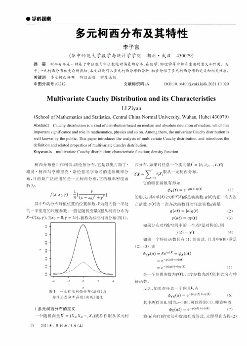
•字餌蓀索多元柯西分布及其特性李子言(华中师范大学数学与统计学学院湖北•武汉430079)摘要柯西分布是一种基于中位数与中位数绝对偏差的分布,在数学、物理学等中都有重要的意义和作用。
其 中,一元柯西分布被大众所熟知,本文以此引入多元柯西分布的分析,初步介绍了多元柯西分布的定义和相关性质。
关键词多元柯西分布特征函数密度函数中图分类号:〇212文献标识码:ADOI : 10.16400/j .cnki .kjdk .2021.10.020Multivariate Cau c h y Distribution and i t s CharacteristicsLI Ziyan(School o f Mathematics and Statistics, Central China Normal University, Wuhan, Hubei 430079)Abstract Cauchy distribution is a kind of distribution based on median and absolute deviation of median , which hasimportant significance and role in mathematics , physics and so on . Among them , the univariate Cauchy distribution is well known by the public . This paper introduces the analysis of multivariate Cauchy distribution , and introduces the definition and related properties of multivariate Cauchy distribution .Keywords multivariate Cauchy distribution ; characteristic function ; density function 柯西分布也叫作柯西-洛伦兹分布,它是以奧古斯丁 • 路易•柯西与亨德里克•洛伦兹名字命名的连续概率分 布,目前最广泛应用的是一元柯西分布,它的概率密度函 数为:/(x ;x 〇-r ) = ^[(^7T 7]其中心为分布峰值位置的位置参数,y 为最大值一半处 的一半宽度的尺度参数。
probability distribution的表达式

Probability distribution是描述随机变量的概率性质的函数,通常用符号P(X)来表示,其中X 表示随机变量。
Probability distribution的表达式通常包括两个部分:概率质量函数(probability mass function)和连续概率分布函数(continuous probability distribution function)。
1. 概率质量函数
对于离散型随机变量,概率质量函数定义为在某个取值x下,该取值出现的概率P(X=x),其表达式为:
P(X=x) = ΣP(X=x') * x' = Σf(x) * x
其中,f(x)表示概率密度函数,x'表示任意实数,求和符号Σ表示对所有可能的取值求和。
2. 连续概率分布函数
对于连续型随机变量,概率密度函数可以看作是连续概率分布函数,其定义域为整个实数轴。
连续概率分布函数的表达式为:
f(x) = P(X ≤x) dx
其中,P(X ≤x)表示随机变量X小于等于x的概率,dx表示对任意实数x的微小区间的长度。
这个表达式可以理解为随机变量X在某个区间[a, b]内的概率等于该区间内所有点的概率的总和。
连续概率分布函数可以用各种函数形式来表示,例如高斯分布函数(也称正态分布函数)的表达式为:
f(x) = 1/(σ√(2π)) * e^(-(x-μ)²/(2σ²))
其中,e是自然常数,σ²是方差,μ是均值。
遗传算法工具箱在弧底梯形明渠正常水深计算中的应用

1 计算弧底梯形明渠正常水深的方法
根据连续方程和谢才公式, 可得到明渠均匀流 的流量计算基本方程为 [ 2] :
2007年 12月 18 日收到 第一作者简介: 叶培 聪 ( 1973) ), 男, 汉族, 安 徽安庆 人, 工程 师, 研究方向: 水利工程设计。
Q = AC R i
( 1)
( 1)式中: Q 为流量 (m3 / s); A 为过 水断面面
1 1+ m2
-1
( 5)
由式 ( 1) ~ 式 ( 5)可见, 弧底梯形断面正常水深的
22 70
科学技术与工程
8卷
计算须求解复杂高次方程, 因而试算法和图表法计 算量大 且精 度不 易 保证。文献 [ 1 ] 对 计 算公 式 ( 1) ~ 式 ( 5) 进行数学变换, 得到其无量纲正常 水深的迭代公式, 从而使得计算过程无需试算, 但 从理论上讲这只能得到原问题的近似解, 且需要构 造收敛的迭代公式和合理选取初值, 而这往往要求 设计人员具有较高的计 算数学理论知 识。本文将
渠道输水工程中的弧底梯形渠道断面, 由于其 水力和结构性能的优越, 已逐步得到推广应用。然 而弧底梯形渠道断面水力计算中的正 常水深求解 无显函数形式的表达公式, 这使得水力计算变得复 杂难求。目前 常用的求解方法 有试算法、图表法、 简便算法、迭代公式法、搜索法 [ 1) 5 ] 等。这些方法的 人工计算量大、计算精度不 高, 或要求 较高的计算 数学的理论知识等, 难以在生产实际中被大规模推 广应用。本文通过对 弧底梯形明渠均 匀流基本方 程的数学变换, 把正常水深的计算问题归结为非线 性优化问题, 再运用以 MATLAB 为平台的遗传算法 工具箱来求解, 试图为计算正常水深提供一种通用 有效的方法。
The Newsvendor Model(非常好的基础知识和推导)

1. Introduction
Early each morning, the owner of a corner newspaper stand needs to order newspapers for that day. If the owner orders too many newspapers, some papers will have to be thrown away or sold as scrap paper at the end of the day. If the owner does not order enough newspapers, some customers will be disappointed and sales and profit will be lost. The newsvendor problem is to find the best (optimal) number of newspapers to buy that will maximize the expected (average) profit given that the demand dis. The newsvendor problem is a one-time business decision that occurs in many different business contexts such as:
1
A stockout is a situation where the demand for one or more units cannot be satisfied immediately from inventory.
Copyright © 2010 Clamshell Beach Press,
(完整word)概率论与数理统计英文版总结,推荐文档

(完整word)概率论与数理统计英⽂版总结,推荐⽂档Sample Space样本空间The set of all possible outcomes of a statistical experiment is called the sample space.Event 事件An event is a subset of a sample space.certain event(必然事件):The sample space S itself, is certainly an event, which is called a certain event, means that it always occurs in the experiment.impossible event(不可能事件):The empty set, denoted by?, is also an event, called an impossible event, means that it never occurs in the experiment. Probability of events (概率)If the number of successes in n trails is denoted by s, and if the sequence of relative frequencies /s n obtained for larger and larger value of n approaches a limit, then this limit is defined as the probability of success in a single trial.“equally likely to occur”------probability(古典概率)If a sample space S consists of N sample points, each is equally likely to occur. Assume that the event A consists of n sample points, then the probability p that A occurs is()np P AN==Mutually exclusive(互斥事件)Two events A and B are said to be independent if()()()P A B P A P B=?IOr Two events A and B are independent if and only if(|)()P B A P B=.Conditional Probability 条件概率The probability of an event is frequently influenced by other events.If 12k ,,,A A A L are events, then12k 121312121()()(|)(|)(|)k k P A A A P A P A A P A A A P A A A A -=??I I L I L I I L I If the events12k ,,,A A A L areindependent, then for any subset12{,,,}{1,2,,}m i i i k ?L L ,1212()()()()m m P A A A P A P A P A i i i i i i =I I L L(全概率公式 total probability)()(|)()i i P B A P B A P A =IUsing the theorem of total probability, we have1()(|)(|)()(|)i i i kjjj P B P A B P B A P B P A B ==∑ 1,2,,i k =L1. random variable definition2. Distribution functionNote The distribution function ()F X is defined on real numbers, not on sample space. 3. Properties The distribution function ()F x of a random variable X has the following properties:3.2 Discrete Random Variables 离散型随机变量geometric distribution (⼏何分布)Binomial distribution(⼆项分布)poisson distribution(泊松分布)Expectation (mean) 数学期望2.Variance ⽅差standard deviation (标准差)probability density function概率密度函数5. Mean (均值)6. variance ⽅差.4.2 Uniform Distribution 均匀分布The uniform distribution, with the parameters a a nd b , has probability density function 1for ,()0 elsewhere,a xb f x b a<=-4.5 Exponential Distribution 指数分布4.3 Normal Distribution正态分布1. Definition4.4 Normal Approximation to the Binomial Distribution (⼆项分布)4.7 C hebyshev’s Theorem (切⽐雪夫定理)Joint probability distribution (联合分布)In the study of probability, given at least two random variables X, Y , ..., that are defined on a probability space, the joint probabilitydistribution for X, Y , ... is a probability distribution that gives the probability that each of X, Y , ... falls in any particular range or discrete set of values specified for that variable. 5.2 C onditional distribution 条件分布Consistent with the definition of conditional probability of events when A is the event X =x and B is the event Y =y , the conditional probability distribution of X given Y =y is defined as(,)(|)()X Y p x y p x y p y =for all x provided ()0Y p y ≠. 5.3 S tatistical independent 随机变量的独⽴性5.4 Covariance and Correlation 协⽅差和相关系数We now define two related quantities whose role in characterizing the interdependence of X and Y we want to examine.理We can find the steadily of the frequency of the events in large number of random phenomenon. And the average of large number of random variables are also steadiness. These results are the law of large numbers.population (总体)A population may consist of finitely or infinitely many varieties. sample (样本、⼦样)中位数Sample Distributions 抽样分布1.sampling distribution of the mean 均值的抽样分布It is customary to write )(X E as X µ and )(X D as 2X σ.Here, ()E X µ= is called the expectation of the mean .均值的期望nX σσ=is called the standard error of the mean. 均值的标准差7.1 Point Estimate 点估计Unbiased estimator(⽆偏估计量)minimum variance unbiased estimator (最⼩⽅差⽆偏估计量)3. Method of Moments 矩估计的⽅法confidence interval----- 置信区间lower confidence limits-----置信下限upper confidence limits----- 置信上限degree of confidence----置信度2.极⼤似然函数likelihood functionmaximum likelihood estimate(最⼤似然估计)8.1 Statistical Hypotheses(统计假设)显著性⽔平Two Types of Errors。
广义中心极限定理 英语
广义中心极限定理英语The Generalized Central Limit TheoremThe central limit theorem is a fundamental concept in probability theory and statistics, which states that the distribution of the sum or average of a large number of independent and identically distributed random variables will tend to a normal distribution, regardless of the underlying distribution of the individual variables. This theorem has far-reaching implications in various fields, including finance, engineering, and the social sciences.While the classical central limit theorem is a powerful tool, it is limited to the case where the random variables are independent and identically distributed. However, in many real-world situations, this assumption may not hold, and the variables may exhibit more complex dependencies or non-identical distributions. This is where the generalized central limit theorem (GCLT) comes into play.The GCLT is a more general version of the central limit theorem that relaxes the assumptions of independence and identical distribution. It states that the distribution of the sum or average of a large number of random variables will converge to a stable distribution,which is a broader class of probability distributions that includes the normal distribution as a special case.The key to understanding the GCLT is the concept of a stable distribution. A stable distribution is a probability distribution that satisfies the following property: the sum of two independent random variables with the same stable distribution is also a random variable with the same stable distribution, up to a scale and location parameter. This property is known as the stability property, and it is the foundation of the GCLT.There are four main parameters that characterize a stable distribution: the index of stability (α), the skewness parameter (β), the scale parameter (σ), and the location parameter (μ). The index of stability, α, is the most important parameter, as it determines the shape of the distribution. When α = 2, the stable distribution reduces to the normal distribution, which is the special case covered by the classical central limit theorem.The GCLT states that if the sum or average of a large number of random variables is properly normalized, then the distribution of the normalized sum or average will converge to a stable distribution as the number of variables goes to infinity. The specific form of the stable distribution depends on the values of the four parameters mentioned above, which in turn depend on the characteristics of theindividual random variables.One of the key advantages of the GCLT is its ability to handle non-independent and non-identically distributed random variables. This is particularly important in many real-world applications, where the assumptions of independence and identical distribution may not be realistic. For example, in financial markets, asset returns often exhibit complex dependencies and non-normal distributions, which can be better captured by the GCLT.Another important aspect of the GCLT is its connection to the concept of heavy-tailed distributions. Heavy-tailed distributions are probability distributions that have a slower decay rate in their tails compared to the normal distribution. These distributions are often observed in various natural and social phenomena, such as the distribution of wealth, the size of earthquakes, and the intensity of internet traffic. The GCLT provides a theoretical framework for understanding the emergence of heavy-tailed distributions in the sum or average of a large number of random variables.In conclusion, the generalized central limit theorem is a powerful and versatile tool in probability theory and statistics. It extends the classical central limit theorem to a broader class of random variables, allowing for more realistic modeling of complex real-world phenomena. The GCLT has important applications in fields such asfinance, engineering, and the social sciences, and its continued study and development is an active area of research.。
科学无国界英语作文

科学无国界英语作文Science knows no borders, and it is this universalitythat has propelled humanity forward in leaps and bounds. From the depths of the ocean to the farthest reaches of the cosmos, the quest for knowledge has united people across continents and cultures, transcending the barriers of language and tradition. The pursuit of science is a testament to our collective curiosity and our desire to understand the world around us.In the realm of medicine, scientific collaboration hasled to groundbreaking discoveries that have saved countless lives. The development of vaccines, for instance, is a global effort that has eradicated diseases and brought hope to millions. Similarly, in the field of technology, the internet, a product of international cooperation, has revolutionized communication and information sharing, connecting us in ways previously unimaginable.The spirit of scientific inquiry is not confined bypolitical boundaries or national interests. It is a collaborative endeavor that thrives on the exchange of ideas and the pooling of resources. When scientists from different countries come together, they bring diverse perspectives and expertise, which enriches the research process andaccelerates innovation.Moreover, the fruits of scientific progress are sharedglobally. Knowledge is disseminated through academic journals, conferences, and collaborative projects, ensuring that advancements benefit all of humanity. This sharing of information is crucial for addressing global challenges suchas climate change, where international cooperation isessential for developing sustainable solutions.However, it is important to recognize that while science itself is borderless, the practice of science is not immuneto geopolitical influences. Funding, access to resources, and the distribution of scientific talent can be uneven, creating disparities that hinder the equitable advancement of knowledge. It is the responsibility of the global communityto address these imbalances and ensure that the pursuit of science remains inclusive and accessible to all.In conclusion, the boundless nature of science is abeacon of hope in a world that is often divided. It serves as a reminder that our common goal of understanding andimproving our world can bring us together, regardless ofwhere we come from. As we continue to explore the unknown,let us do so with an open mind and a collaborative spirit,for it is in this unity that we find our greatest strength.。
TransverseSpinPh...

Transverse Spin Physics:Recent DevelopmentsFeng Yuan1,2∗1-Nuclear Science Division,Lawrence Berkeley National Laboratory,Berkeley,CA94720,USA 2-RIKEN BNL Research Center,Brookhaven National Laboratory,Upton,NY11973,USATransverse-spin physics has been very active and rapidly developing in the last fewyears.In this talk,I will briefly summarize recent theoretical developments,focusingon the associated QCD dynamics in transverse spin physics.There have been strong experimental interests on transverse spin physics around the world,from the deep inelastic scattering experiments such as the HERMES collaboration at DESY,SMC at CERN,and Hall A and CLAS at JLab,the proton-proton collider experiment from RHIC at Brookhaven,and the very relevant e+e−annihilation experiment from BELLE at KEK.One of the major goals in transverse spin physics is to study the quark transversity distribution,the last unknown leading-twist quark distribution in nucleon.As discussed by several talks in this conference,we can study the quark transversity distributions from many processes[1,2,3,4,5],such as the double transverse spin asymmetry in Drell-Yan lepton pair production in pp collision,single hadron and two hadron production in semi-inclusive deep inelastic scattering,and other processes.We are now starting to have afirst glimpse about the quark transversity distribution from the experiments(see from example[5]).Besides the quark transversity distribution,the transverse spin physics also opened a new window to explore the partonic structure of nucleon,the so-called transverse momen-tum dependent(TMD)parton distributions[4].TMD parton distribution is an exten-sion to the usual Feynman parton distributions.These distributions allow us to study the three-dimension picture of partons inside the nucleon,and they are also closely related to the generalized parton distributions[6]and the parton orbital angular momenta.Es-pecially,the single transverse spin asymmetry(SSA)phenomena in high energy hadronic processes have attracted many theoretical and experimental investigations.The SSA is defined as the asymmetry when one of the hadrons’transverse spin isflipped,A N∼(dσ(S⊥)−dσ(−S⊥))/(dσ(S⊥)−dσ(−S⊥)).It has been a great theoretical challenge in the understanding of these phenomena.This is because the leading partonic contribution to the SSA vanish in the leading order,whereas the experimental observation show that these SSAs are in tens of percentage in the forward scattering of the polarized nucleon.Recent theoretical developments have made great progress in the exploration of the underlying physics for the single spin phenomena.It is impossible to cover all these exciting physics in this short talk.Rather,I would like to focus on one important subject,i.e.,the nontrivial QCD dynamics associated with transverse spin physics:the QCD factorization, and the universality of the parton distributions and fragmentation functions.Among those TMD parton distributions and fragmentation functions,two functions have been mostly discussed:the Sivers quark distribution and the Collins fragmentation func-tion.The Sivers quark distribution represents a distribution of unpolarized quarks in a ∗This work was supported in part by the U.S.Department of Energy under contract DE-AC02-05CH11231.We are grateful to RIKEN,Brookhaven National Laboratory and the U.S.Department of Energy(contract number DE-AC02-98CH10886)for providing the facilities essential for the completion of this work.transversely polarized nucleon,through a correlation between the quark’s transverse mo-mentum and the nucleon polarization vector.The Collins function represents a correlation between the transverse spin of the fragmenting quark and the transverse momentum of the hadron relative to the “jet axis”in the fragmentation process.Although they both belong to the so-called “naive-time-reversal-odd”functions,they do have different universality prop-erties.For the quark Sivers function,because of the initial/final state interaction difference,they differ by signs for the SIDIS and Drell-Yan processes [7,8,9,10].On the other hand,there have been several studies showing that the Collins function is universal between differ-ent processes,primarily in the SIDIS and e +e −annihilation [11,12,13,14],and recently in pp collisions [15].In the following,I will take the example of the Collins contribution to the azimuthal asymmetric distribution of hadrons inside a high energy jet in the transversely polarized pp collision to demonstrate this universality property,p (P A ,S ⊥)+p (P B )→jet (P J )+X →H (P h )+X ,(1)where a transversely polarized proton with momentum P A scatters on another proton with momentum P B ,and produces a jet with momentum P J .The three momenta of P A ,P B and P J form the so-called reaction plane.Inside the produced jet,the hadrons are distributed around the jet axis,where we define transverse momentum P hT relative to the jet axis.The correlation between P hT and the polarization vector S ⊥introduces the Collins contribution to the single spin asymmetry in this process.Figure 1:Gluon exchange diagrams contributions to the Collins asymmetry in pp collisions.The short bars indicate the pole contributions to the phase needed for a non-vanishing SSA.The additional two cuts in (d)cancel out each other.We need to generate a phasefrom the scattering amplitudes tohave a non-vanishing SSA.If thephase comes from the vertex asso-ciated with the fragmenting quarkand the final state hadron,or from the dressed quark propa-gator,it is easy to argue the universality of the Collins func-tion between this process and theSIDIS/e +e −process,because theyare the same.The main issueof the universality discussion con-cerns the extra gluon exchangecontribution between the specta-tor of the fragmentation process and hard partonic part.In Fig.2,we have shown all these inter-actions for a particular partonic channel qq →qq contribution,in-cluding the gluon attachments to the incident quarks (a,c),and final state balancing quark (d)and theinternal gluon propagator (b).The contributing phases of the diagrams in Fig.2come from the cuts through the internal propagators in the partonic scattering amplitudes.In Fig.2,we labeled these cut-poles by short bars in the diagrams.From the calculations,we will find that all these poles come from a cut through the exchanged gluon and the fragmenting quarkin each diagram,and all other contributions either vanish or cancel out each other.For ex-ample,in Fig.2(d),we show two additional cuts,which contribute however opposite to each other and cancel out completely.Therefore,by using the Ward identity at this particular order,thefinal results for all these diagrams will sum up together into a factorized form, where the cross section is written as the hard partonic cross section for q(S⊥)q →q(s⊥)q subprocess multiplied by a Collins fragmentation function.The exchanged gluon in Fig.2 is now attaching to a gauge link from the fragmentation function definition.Similar calcu-lations can be performed for the other two processes SIDIS and e+e−annihilation,and the same Collins function will be observed.This argument can also be extended to two-gluon exchange diagrams[15].The key steps in the above derivation are the eikonal approximation and the Ward iden-tity.The eikonal approximation is valid when we calculate the leading power contributions in the limit of P hT P J.The Ward identity ensure that when we sum up the diagrams with all possible gluon attachments we shall get the eikonal propagator from the gauge link in the definition of the fragmentation function.The most important point to apply the Ward identity in the above analysis is that the eikonal propagator does not contribute to the phase needed to generate a nonzero SSA.This observation is very different from the SSAs associated with the parton distributions, where the eikonal propagators from the gauge link in the parton distribution definition play very important role[4,7,8,9,10,16].It is the pole of these eikonal propagators that contribute to the phase needed for a nonzero SSA associated with the naive-time-reversal-odd parton distributions,which also predicts a sign difference for the quark Sivers function between the SIDIS and Drell-Yan processes.More complicated results have been found for the SSAs in the hadronic dijet-correlation[17,18],where a normal TMD factorization breaks down[19].The reason is that the eikonal propagators from the initial andfinal state interactions in dijet-correlation process do contribute poles in the cross section[18,19]. Because of this,the Ward identity is not applicable,and the standard TMD factorization breaks down,although a modified factorization may be valid if we modify the definition of the TMD parton distributions to take into account all the initial andfinal state interaction effects[17].In particular,there is a sign change between the SSAs in SIDIS and Drell-Yan pro-cesses[7,8],Sivers SSA|DY=−Sivers SSA|DIS.(2) This nontrivial result of the opposite signs between the above two processes will still hold when gluon radiation contributions are taken into account,where the large transverse mo-mentum Sivers function is generated from the twist-three quark-gluon correlation func-tion[20,21].It is of crucial to test this nontrivial QCD predictions by comparing the SSAs in these two processes.The Sivers single spin asymmetry in SIDIS process has been observed by the HERMES collaboration,and the planned Drell-Yan measurement at RHIC and other facility will test this prediction.Another interesting probe for the initial/final state interaction effects is the SSA in heavy quark and antiquark production in hadronic process.Because the heavy quark and antiquark can be detected by their decay products,their SSAs can be measured separately.The heavy quark and antiquark produced in short distance partonic processes will experience different final state interactions with the nucleon spectator due to their different color charges,and therefore the SSAs for heavy quark and antiquark will be different.Detailed calculationsshow that the difference could be as large as a factor of3if the quark-antiquark channel contribution dominates[22].In summary,the universality of the parton distribution and fragmentation functions are very different in the single transverse spin asymmetry.These properties are still under theoretical and experimental investigations.These important physics,together with other exciting features have shown that the transverse spin physics is playing a very important role in the strong interaction physics for hadronic spin physics.We will learn more about QCD dynamics and nucleon structure from these studies.References[1]K.Tanaka,these proceedings.[2]G.Goldstein,these proceedings.[3]M.Radici,these proceedings.[4]P.Mulders,these proceedings.[5] A.Prokudin,these proceedings.[6]T.Teckentrup,these proceedings.[7]S.J.Brodsky,D.S.Hwang and I.Schmidt,Phys.Lett.B530,99(2002);Nucl.Phys.B642,344(2002).[8]J.C.Collins,Phys.Lett.B536,43(2002).[9]X.Ji and F.Yuan,Phys.Lett.B543,66(2002);A.V.Belitsky,X.Ji and F.Yuan,Nucl.Phys.B656,165(2003).[10] D.Boer,P.J.Mulders and F.Pijlman,Nucl.Phys.B667,201(2003).[11] A.Metz,Phys.Lett.B549,139(2002).[12]J.C.Collins and A.Metz,Phys.Rev.Lett.93,252001(2004).[13]L.P.Gamberg,A.Mukherjee and P.J.Mulders,Phys.Rev.D77,114026(2008).[14]L.Gamberg,these proceedings.[15] F.Yuan,Phys.Rev.Lett.100,032003(2008);Phys.Rev.D77,074019(2008).[16] C.Pisano,these proceedings.[17] C.J.Bomhof,P.J.Mulders and F.Pijlman,Phys.Lett.B596,277(2004);Eur.Phys.J.C47,147(2006);JHEP0702,029(2007);A.Bacchetta,C.J.Bomhof,P.J.Mulders and F.Pijlman,Phys.Rev.D72,034030(2005);C.J.Bomhof and P.J.Mulders,arXiv:0709.1390[hep-ph].[18]J.W.Qiu,W.Vogelsang and F.Yuan,Phys.Lett.B650,373(2007);Phys.Rev.D76,074029(2007);W.Vogelsang and F.Yuan,Phys.Rev.D76,094013(2007).[19]J.Collins and J.W.Qiu,Phys.Rev.D75,114014(2007);J.Collins,arXiv:0708.4410[hep-ph].[20]X.Ji,J.W.Qiu,W.Vogelsang and F.Yuan,Phys.Rev.Lett.97,082002(2006);Phys.Rev.D73,094017(2006);Phys.Lett.B638,178(2006).[21] A.Bacchetta,these proceedings.[22] F.Yuan and J.Zhou,arXiv:0806.1932[hep-ph].。
cumulative probability function
Cumulative Probability FunctionIntroductionThe cumulative probability function (CPF) is a fundamental concept in probability theory and statistics. It is used to calculate the probability that a random variable takes on a value less than or equal to a given value. In other words, the CPF gives us the cumulative distribution function (CDF) of a random variable.DefinitionThe cumulative probability function, denoted as F(x), of a random variable X is defined as the probability that X takes on a value less than or equal to x. Mathematically, it can be expressed as:F(x) = P(X ≤ x)Properties of CPF1.The range of the CPF is between 0 and 1, inclusive. This isbecause probabilities are always between 0 and 1.2.The CPF is a non-decreasing function. As x increases, thecumulative probability also increases.3.The CPF is a right-continuous function. This means that theprobability of X taking on a particular value is equal to thedifference in cumulative probabilities between that value and the next smallest value.Calculation of CPFThe CPF can be calculated for different types of random variables, including discrete and continuous random variables.Discrete Random VariablesFor a discrete random variable, the CPF can be calculated by summing up the probabilities of all values less than or equal to x. Let’s cons ider an example of a fair six-sided die:X 1 2 3 4 5 6P(X) 1/6 1/6 1/6 1/6 1/6 1/6To calculate the CPF for this die, we sum up the probabilities as follows:F(1) = P(X ≤ 1) = 1/6 F(2) = P(X ≤ 2) = 2/6 F(3) = P(X ≤ 3) = 3/6 F(4) = P(X ≤ 4) = 4/6 F(5) = P(X ≤ 5) = 5/6 F(6) = P(X ≤ 6) = 6/6 = 1Continuous Random VariablesFor a continuous random variable, the CPF can be calculated using the probability density function (PDF) of the variable. The CPF is then obtained by integrating the PDF over the range from negative infinity to x.Let’s consider an example of a continuous random variable X with a normal distribution:PDF of X ~ N(μ, σ^2):f(x) = (1 / (σ * sqrt(2π))) * exp(-(x - μ)^2 / (2σ^2))To calculate the CPF for a specific value x, we integrate the PDF from negative infinity to x:F(x) = ∫[from -∞ to x] f(t) dtApplications of CPFThe CPF has various applications in probability theory, statistics, and data analysis. Some of the key applications are:1.Probability calculations: The CPF allows us to calculate theprobability of a random variable taking on a specific value orfalling within a certain range.2.Hypothesis testing: The CPF is used in hypothesis testing todetermine the significance level of a test statistic.3.Confidence intervals: The CPF is used to calculate confidenceintervals for a population parameter based on a sample.4.Survival analysis: The CPF is used in survival analysis toestimate the probability of an event occurring before a certaintime.5.Risk assessment: The CPF is used in risk assessment to calculatethe cumulative probability of a particular event or outcome.ConclusionThe cumulative probability function is a powerful tool in probability theory and statistics. It provides a way to calculate the cumulative distribution function of a random variable and has various applications in different fields. Understanding the properties and calculation of the CPF is essential for conducting probabilistic analyses and making informed decisions based on probabilities.。
伍德里奇《计量经济学导论--现代观点》2

΄ ΅ A ϭ
2 Ϫ4
Ϫ1 5
7 0
(D.1)
where a13 ϭ 7. The shorthand A ϭ [aij] is often used to define matrix operations.
DEFINITION D.2 (Square Matrix) A square matrix has the same number of rows and columns. The dimension of a square matrix is its number of rows and columns.
Given any real number ␥ (often called a scalar), scalar multiplication is defined as ␥A ϵ [␥aij], or
΄ ␥a11 ␥a21 ␥A ϭ ...
␥a12 ␥a22
... ...
΅␥a1n
␥a2n .
␥am1 ␥am2 . . . ␥amn
For example, if ␥ ϭ 2 and A is the matrix in equation (D.1), then
΄ ΅ ␥A ϭ
4 Ϫ8
Ϫ2 10
14 0.
Matrix Multiplication
To multiply matrix A by matrix B to form the product AB, the column dimension of A must equal the row dimension of B. Therefore, let A be an m ϫ n matrix and let B be an n ϫ p matrix. Then matrix multiplication is defined as
slutsky 定理

slutsky 定理Slutsky定理是经济学中一个基本的定理,它描述了随机变量序列的极限分布。
该定理由Eugen Slutsky在1927年提出,被认为是概率论和经济学中最重要的定理之一。
本文将详细介绍Slutsky定理的定义、证明、应用及其在经济学中的作用。
一、定义Slutsky定理描述了两个随机变量序列的极限分布之间的关系。
具体来说,假设有两个随机变量序列Xn和Yn,满足以下条件:1. Xn和Yn都是随机变量序列;2. Xn和Yn收敛于相应的随机变量X和Y;3. 对于任意实数t,有limn→∞P(Xn≤t)=limn→∞P(X≤t)和limn→∞P(Yn≤t)=limn→∞P(Y≤t)。
则可以得到以下结论:1. Xn+Yn收敛于X+Y;2. XnYn收敛于XY;3. 如果Y不等于0,则Xn/Yn收敛于X/Y。
二、证明Slutsky定理可以通过利用连续映射定理证明。
具体来说,我们可以将X和Y表示为函数f(x)和g(x)关于x的连续函数,然后利用连续映射定理得到Xn和Yn的极限分布。
对于第一条结论,我们可以使用以下证明方法:设Zn=Xn+Yn,则有:P(Zn≤t)=P(Xn+Yn≤t)=∫∫I(x+y≤t)fXn(x)fYn(y)dxdy其中,I(x+y≤t)为指示函数。
将fXn(x)和fYn(y)表示为关于x和y的连续函数f(x)和g(y),则有:P(Zn≤t)=∫∫I(x+y≤t)f(x)g(y)dxdy由于f(x)和g(y)都是连续函数,因此可以使用Fubini定理交换积分顺序,得到:P(Zn≤t)=∫∞−∞(∫t−xf(x)g(t−x−y)dy)dx由于X和Y收敛于相应的随机变量,因此可以得到:lim n→∞P(Zn≤t)=limn→∞(∫∞−∞(∫t−xfX(x)fY(t−x−y)dy)dx)= ∫∞−∞(limn→∞(F(X)(x))limn→∞(G(Y)(t−x)))dx= ∫−∞^+ ∞F(X)(x)dG(Y)(t−x)= F(X+Y)(t)因此,我们得到了结论:Zn=Xn+Yn收敛于X+Y。
Scale-Free Networks
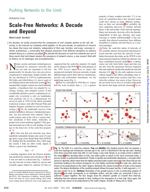
PERSPECTIVEScale-Free Networks:A Decade and BeyondAlbert-LászlóBarabásiFor decades,we tacitly assumed that the components of such complex systems as the cell,the society,or the Internet are randomly wired together.In the past decade,an avalanche of research has shown that many real networks,independent of their age,function,and scope,converge to similar architectures,a universalitythat allowed researchers from different disciplines to embrace network theory as a common paradigm.The decade-old discovery of scale-free networks was one of those events that had helped catalyze the emergence of network science,a new research field with its distinct set of challenges and accomplishments.Nature,society,and many technologies are sustained by numerous networks that are not only too important to fail butparadoxically for decades have also proved too complicated to understand.Simple models,like the one introduced in 1959by mathematicians Pál Erd ős and Alfréd Rényi (1),drove much of our thinking about interconnected systems.They assumed that complex systems are wired randomly together,a hypothesis that was adopted by so-ciology,biology,and computer science.It had considerable predictive power,explaining for ex-ample why everybody is only six handshakes from anybody else (2–5),a phenomenon ob-served as early as 1929(2)but which resonated in physical sciences only after Duncan Watts and Stephen Strogatz extended its reach beyond so-ciology (5).Yet,the undeniable success of the random hypothesis did pose a fundamental ques-tion:Are real networks truly random?That is,could systems such as the cell or a society func-tion seamlessly if their nodes,molecules,or people were wired randomly together?This ques-tion motivated our work as well,leading 10years ago to the discovery of the scale-free property (6,7).Our first clue that real networks may show manifestly nonrandom features also came 10years ago from a map of the World Wide Web (WWW)(8),finding that the probability that a Web page has exactly k links (in other words,degree k )follows a power law distributionP (k )~k-g(1)a stunning departure from the Poisson distribu-tion predicted by random network theory (1).Yet,it was not until we realized that Eq.1character-izes the network of actors linked by movies and scientific papers linked by citations (9)that wesuspected that the scale-free property (6)might not be unique to the WWW.The main purpose of the 1999Science paper was to report this unexpected similarity between networks of quite different nature and to show that two mechanisms,growth and preferential attachment,are the underlying causes (Fig.1).When we concluded in 1999that we “expect that the scale invariant state […]is a genericproperty of many complex networks ”(7),it was more of a prediction than a fact,because nature could have chosen as many different architec-tures as there are networks.Yet,probably the most surprising discovery of modern network theory is the universality of the network topology:Many real networks,from the cell to the Internet,independent of their age,function,and scope,converge to similar architectures.It is this uni-versality that allowed researchers from different disciplines to embrace network theory as a com-mon paradigm.Today,the scale-free nature of networks of key scientific interest,from protein interactions to social networks and from the network of inter-linked documents that make up the WWW to the interconnected hardware behind the Internet,has been established beyond doubt.The evidence comes not only from better maps and data sets but also from the agreement between empirical data and analytical models that predict the network structure (10,11).Yet,the early euphoria was not without negative side effects,prompting some re-searchers to label many systems scale-free,even when the evidence was scarce at best.However,the net result was to force us to better understand the factors that shape network structure.For ex-Pushing Networks to the LimitCenter for Complex Network Research,Department of Physics,Biology,and Computer Science,Northeastern University,Boston,MA 02115,USA.Department of Medicine,Harvard Medical School and Center for Cancer Systems Biology,Dana Farber Cancer Institute,Boston,MA 02115,USA.E-mail:alb@Fig.1.The birth of a scale-free network.(Top and Middle )The simplest process that can produce a scale-free topology was introduced a decade ago in (6),and it is illustrated in the top two rows.Starting from three connected nodes (top left),in each image a new node (shown as an empty circle)is added to the network.When deciding where to link,new nodes prefer to attach to the more connected nodes,a process known as preferential attachment.Thanks to growth and preferential attachment,a rich-gets-richer process is observed,which means that the highly connected nodes acquire more links than those that are less connected,leading to the natural emergence of a few highly connected hubs.The node size,which was chosen to be proportional to the node ’s degree,illustrates the natural emergence of hubs as the largest nodes.The degree distribution of the resulting network follows the power law (Eq.1)with exponent g =3.See also movies S1to S3.(Bottom )Illustration of the growth process in the co-authorship network of physicists.Each node corresponds to an individual author,and two nodes are connected if they co-authored a paper together.The four images show the network ’s growth at 1-month time intervals,indicating how the network expands in time,leading to the emergence of a clear hub.Once again,the node size was chosen to be proportional to the node ’s degree.[Credit:D.Wang and G.Palla]24JULY 2009VOL 325SCIENCE412 o n J u l y 24, 2009w w w .s c i e n c e m a g .o r g D o w n l o a d e d f r o mample,although the randomly bonded atoms in amorphous materials form a fascinating network,we now know that it does not display either the small-world (12)or the scale-free property,thanks to the chemical constraints the bonds must obey (13).Lastly,the topologies of several networks of considerable interest,like the neural-level map of a mammalian brain,remain to be elucidated,rep-resenting an area where we need both data and generative models (14).A legacy of the scale-free property is the re-alization that the structure and the evolution of networks are inseparable (6).Indeed,traditional network models aimed to connect a fixed number of nodes with cleverly placed links.The scale-free property forced us to acknowledge that networks constantly change because of the arrival of nodes and links (Fig.1).In other words,to explain a system ’s topology we first need to describe how it came into being.The impact of network theory could have been limited if not for a series of findings that under-lined the perils of ignoring network topology.Take,for example,the discovery of Romualdo Pastor-Satorras and Alessandro V espignani that on a scale-free network the epidemic threshold converges to zero (15).It has long been known that only viruses whose spreading rate exceeds a critical threshold can survive in the population.Whereas the spread-ing rate captures the transmission dynamics,the threshold is determined by the topology of the network on which the virus spreads.Therefore,the vanishing threshold means that in scale-free networks even weakly virulent viruses can spread unopposed,a finding that affects all spreading processes,from AIDS to computer viruses.Simi-larly,the finding of Shlomo Havlin and collab-orators (16)that in scale-free networks the overall network connectivity does not vanish under random node removal explained the exceptional robustness of real networks to random node failures (17).As a proof of the coherency of the emerging theory,both of these discoveries (15,16)were reduced to the same mathematical property,the diverging second moment of the degree distribution (Eq.1),a unique feature of scale-free networks (6).Lately these features are of great interest,given the increasing concern about the vulnerability of real networks (such as power grids and the Internet)to attack and the realiza-tion that targeting hubs can be massively dis-ruptive (17,18).It is clear that no networks seen in nature or technology are completely random —that is,mech-anisms beyond randomness shape their evolution.The universality of various topological character-istics,from degree distributions (6)to degree correlations (19–21),motifs (22),and commu-nities (23–25),is used as a springboard to study diverse phenomena and to make predictions.With that,network theory has fundamentally reshaped our understanding of complexity.Indeed,al-though we continue to lack a universally agreed-on definition of complexity,the role of networks in this area is obvious:All systems perceived to be complex,from the cell to the Internet and from social to economic systems,consist of an extra-ordinarily large number of components that inter-act via intricate networks.To be sure,we were aware of these networks before.Y et,only recently have we acquired the data and tools to probe their topology,helping us realize that the underlying connectivity has such a strong impact on a system ’s behavior that no approach to complex systems can succeed unless it exploits the network topology.In many ways,the demands of a future theory of complexity are obvious:We need to understand the behavior of the systems that we perceive as being complex.We need to be able to predict how the Internet responds to attacks and traffic jams or how the cell reacts to changes in its en-vironment.To make progress in this direction,we need to tackle the next frontier,which is to under-stand the dynamics of the processes that take place on networks.The problem is that we have almost as many dynamical phenomena as there are com-plex systems.For example,biologists study re-action kinetics on metabolic networks;computer scientists monitor the flow of information on com-puter networks;and epidemiologists,sociologists,and economists explore the spread of viruses and ideas on social networks.Is there a chance that,despite their diversity,these dynamical processes share some common characteristics?I suspect that such commonalities do exist;we just have not yet found the framework to unveil their univer-sality.If we do,combined with the universality of the network topology,we may soon have some-thing that could form the foundation of a theory of complexity.Can we keep the momentum and achieve this in the next decade or so?Perhaps —in my view the bottlenecks are mainly data driven.Indeed,the sudden emergence of large and reliable network maps drove the development of network theory during the past decade.If data of similar detail capturing the dynamics of processes taking place on networks were to emerge in the coming years,our imagination will be the only limitation to progress.If I dare to make a prediction for the next decade,it is this:Thanks to the proliferation of the many electronic devices that we use on a daily basis,from cell phones to Global Position-ing Systems and the Internet,that capture every-thing from our communications to our whereabouts (26,27),the complex system that we are most likely to tackle first in a truly quantitative fashion may not be the cell or the Internet but rather society itself.Today the understanding of networks is a com-mon goal of an unprecedented array of traditional disciplines:Cell biologists use networks to make sense of signal transduction cascades and metab-olism,to name a few applications in this area;computer scientists are mapping the Internet andthe WWW;epidemiologists follow transmission networks through which viruses spread;and brain researchers are after the connectome,a neural-level connectivity map of the brain.Although many fads have come and gone in complexity,one thing is increasingly clear:Interconnectivity is so fundamental to the behav-ior of complex systems that networks are here to stay.References and Notes1.P.Erd ős,A.Rényi,Publ.Math.(Debrecen)6,290(1959).2.F.Karinthy,in The Structure and Dynamics of Networks ,M.Newman,A.-L.Barabasi,D.Watts,Eds.(Princeton Univ.Press,Princeton,NJ,2006).gram,Psychol.Today 2,60(1967).4.I.Pool,M.Kochen,works 1,1(1978).5.D.J.Watts,S.H.Strogatz,Nature 393,440(1998).6.A.-L.Barabási,R.Albert,Science 286,509(1999).7.In a random network,the average node sets the scale of the network,which means that most nodes have about the same number of links as the average node.For networks that follow Eq.1,for g <3the second moment of the distribution diverges,which means that the average is not characteristic because the error bars characterizing our uncertainty about its value are infinite.These networks lack a characteristic scale;hence,they are called scale-free.Formally,networks whose degree distribution follows Eq.1are called scale-free networks.8.R.Albert,H.Jeong,A.-L.Barabási,Nature 401,130(1999).9.S.Redner,Eur.Phys.J.B 4,131(1998).10.G.Caldarelli,Scale-Free Networks (Oxford Univ.Press,Oxford,2007).11.S.N.Dorogovtsev,J.F.F.Mendes,Evolution of Networks:From Biological Networks to the Internet and WWW (Oxford Univ.Press,Oxford,2003).12.The small-world property refers to the fact that in manynetworks the average node to node distance is rather small,of the order of log N ,where N is the number of nodes in the network.13.L.A.N.Amaral,A.Scala,M.Barthelemy,H.E.Stanley,Proc.Natl.Acad.Sci.U.S.A.97,11149(2000).14.E.T.Bullmore,O.Sporns,Nat.Rev.Neurosci.10,186(2009).15.R.Pastor-Satorras,A.Vespignani,Phys.Rev.Lett.86,3200(2001).16.R.Cohen,K.Reez,D.Ben-Avraham,S.Havlin,Phys.Rev.Lett.85,4626(2000).17.R.Albert,H.Jeong,A.-L.Barabási,Nature 406,378(2000).18.A.E.Motter,Phys.Rev.Lett.93,098701(2004).19.M.E.J.Newman,Phys.Rev.Lett.89,208701(2002).20.R.Pastor-Satorras,A.Vázquez,A.Vespignani,Phys.Rev.Lett.87,258701(2001).21.S.Maslov,K.Sneppen,Science 296,910(2002)o et al .,Science 298,824(2002).23.M.E.J.Newman,Phys.Today 61,33(2008).24.G.Palla,I.Derényi,I.Farkas,T.Vicsek,Nature 435,814(2005).25.J.Reichardt,S.Bornholdt,Phys.Rev.E 74,016110(2006).26.A.Vespignani,Science 325,425(2009).27.M.C.González,C.A.Hidalgo,A.-L.Barabási,Nature453,779(2008).Supporting Online Material/cgi/content/full/325/5939/412/DC1Movies S1to S310.1126/science.1173299 SCIENCEVOL 32524JULY 2009413SPECIAL SECTIONo n J u l y 24, 2009w w w .s c i e n c e m a g .o r g D o w n l o a d e d f r o m。
概化理论(2)

所得到的方差分量估计值足以计算D研究的误
差和G、φ系数即可。
返回
总 结-----GT的特色
一次量化分析就能估计出各个误差来源 的大小,并且为研究者提供了使测量信 度最优化的方法 把整个研究细分成了概化(G)研究和 决策(D)研究 在结果解释上对相对决策和绝对决策作 了区分
两个全域
随机平行假设
可接受的观察全域(universe of
admissible abservations) 全域分数(universal score)
概化全域(universe of generalization)
G研究结果的解释
方差分量的解释
绝对解释:根据方差分量的平方根的大 小来解释
相对解释:各方差分量占总方差的百分 比
ˆ
2 pi
,e
EMSr
研究过程2- D研究
利用G研究结果来计算D研究各种可能的 设计方案的误差方差和概化系数。
研究者可以根据需要变换侧面的水平数, 或者更改D研究的设计形式,变交叉为嵌 套等等,再来计算水平数值不同或者不 同设计形式时的指标。
误差和概化系数计算公式
pxi
2
2
Rle e
ni
A 2 bs(i2e 2)ni
完全随机交叉设计
两个侧面之间、侧面与被试之间都是交叉的,
记作pxixj,
采用pxixj设计的G、D研究
变异来源 方差分量 G研究 D研究 举例 小结
变异来源
p
pi
pj
pij,e
i ij
j
pxixj
2 p
2 pi
2
2 pj
pij ,e
2 i
2 ij
2 j
- 1、下载文档前请自行甄别文档内容的完整性,平台不提供额外的编辑、内容补充、找答案等附加服务。
- 2、"仅部分预览"的文档,不可在线预览部分如存在完整性等问题,可反馈申请退款(可完整预览的文档不适用该条件!)。
- 3、如文档侵犯您的权益,请联系客服反馈,我们会尽快为您处理(人工客服工作时间:9:00-18:30)。
Universality of the Distribution Functions of Random Matrix Theory
Craig A. Tracy Department of Mathematics and Institute of Theoretical Dynamics University of California, Davis, CA 95616, USA e-mail address: tracy@ Harold Widom Department of Mathematics University of California, Santa Cruz, CA 95064, USA e-mail address: widom@ February 9, 2008
3.1
Bulk Scaling Limit
Denote the density of eigenvalues at the point x0 by ρ(x0 ). It is customary in the limit N → ∞ to scale distances so that the resulting density is one. Precisely, we define ξ = ρN (x0 )(x − x0 ), x0 independent of N , and consider the limit N → ∞, x → x0 , such that ξ is fixed. By requiring x0 to be independent of N , we are choosing a point in the “bulk” of the spectrum and are examining the local statistics of the eigenvalues in some small neighborhood of the point x0 . In this limit, and for β = 2, we are led to the Fredholm determinant of the operator on L2 (0, s) whose kernel is the famous sine-kernel [11, 10] K (ξ, ξ ′ ) := 1 sin π (ξ − ξ ′ ) . π ξ − ξ′
The exact computation of n-point correlation functions is generally an open problem for most “solvable” models. In the special case of the 2D Ising model, the n-point functions (in the scaling limit) are expressible in terms of solutions to integrable differential equations [6, 7, 8]. The Wigner-Dyson theory of random matrices [9, 10] is a second class of statistical models where integrable differential equations and n-point correlations (or more precisely, level-spacing distributions) are related. This paper reviews some of these relationships. In section 2 we define the basic objects of random matrix theory (RMT). In section 3 we recall the bulk scaling limit and the edge scaling limit and express various distribution functions in terms of Painlev´ e transcendents. In section 4 we discuss the universality of these distribution functions.
Dedicated to James B. McGuire on the occasion of his sixty-fifth birthday.
1
Introduction
Statistical mechanical lattice models are called solvable if their associated Boltzmann weights satisfy the factorization or star-triangle equations of McGuire [1], Yang [2] and Baxter [3]. For such models the free energy per site and the one-point correlations in the thermodynamic limit are expressible in closed form [4]. There exists a deep mathematical structure [4, 5] underlying these solvable models; and near critical points, a wider applicability than one would initially expect. This last phenomenon, called universality , has its mathematical roots in the strong law of large numbers and the central limit theorems of probability theory and its physical origins in critical phenonmena and conformal field theory. 1
2
3
If Eβ (0; s) denotes the limiting value of EN β (0; (−t, t)) in the bulk scaling limit with the scaled length of J set equal to s, then [10, 16, 19] E1 (0; s) = E2 (0; s) = E4 (0; s/2) = det (I − K+ ) , det (I − K ) , 1 (det (I − K+ ) + det (I − K− )) 2
where CN β is a normalization constant and 1 for GOE, 2 for GUE, β := 4 for GSE.
x j ∈J
probability no eigenvalues lie in J ,
are particularly interesting [10]. The simplest choices of J are (a, b) and (t, ∞). In the first instance the mixed second partial derivative EN β (0; J ) with respect to a and b gives the spacing distribution between consecutive eigenvalues; and in the second case, FN β (t) := EN β (0; (t, ∞)) is the distribution function for the largest eigenvalue. 2
Random Matrix Models
In the Gaussian models [9, 10], the probability density that the eigenvalues lie in infinitesimal intervals about the points x1 , . . . , xN is given by PN β (x1 , . . . , xN ) = CN β e− 2 β
1
x2 i j<k
|xj − xk |β ,
(1)
We recall that for β = 1 the matrices are N × N real symmetric, for β = 2 the matrices are N × N complex Hermitian, and for β = 4 the matrices are 2N × 2N self-dual Hermitian matrices. (For β = 4 each eigenvalue has multiplicity two.) In each case the eigenvalues are real. In RMT the probabilities EN β (0; J ) := = ··· PN β (x1 , . . . , xN ) dx1 · · · dxN ,
Observe that the kernel is translationally invariant and independent of the point x0 . It is a result of Jimbo et al. [15] that
πs
det (I − λK ) = exp where σ satisfies the differential equation