Modeling of Magnetization and Intrinsic Properties of Ideal Type-II Superconductors
Chapter6 凝聚态物理导论(中科院研究生院)
Chapter 6 Magnetism of MatterThe history of magnetism dates back to earlier than 600 B.C., but it is only in the twentieth century that scientists have begun to understand it, and develop technologies based on this understanding. Magnetism was most probably first observed in a form of the mineral magnetite called lodestone, which consists of iron oxide-a chemical compound of iron and oxygen. The ancient Greeks were the first known to have used this mineral, which they called a magnet because of its ability to attract other pieces of the same material and iron.The Englishman William Gilbert(1540-1603) was the first to investigate the phenomenon of magnetism systematically using scientific methods. He also discovered that Earth is itself a weak magnet. Early theoretical investigations into the nature of Earth's magnetism were carried out by the German Carl Friedrich Gauss(1777-1855). Quantitative studies of magnetic phenomena initiated in the eighteenth century by Frenchman Charles Coulomb(1736-1806), who established the inverse square law of force, which states that the attractive force between two magnetized objects is directly proportional to the product of their individual fields and inversely proportional to the square of the distance between them.Danish physicist Hans Christian Oersted(1777-1851) first suggested a link between electricity and magnetism. Experiments involving the effects of magnetic and electric fields on one another were then conducted by Frenchman Andre Marie Ampere(1775-1836) and Englishman Michael Faraday(1791-1869), but it was the Scotsman, James Clerk Maxwell(1831-1879), who provided the theoretical foundation to the physics of electromagnetism in the nineteenth century by showing that electricity and magnetism represent different aspects of the same fundamental force field. Then, in the late 1960s American Steven Weinberg(1933-) and Pakistani Abdus Salam(1926-96), performed yet another act of theoretical synthesis of the fundamental forces by showing that electromagnetism is one part of the electroweak force. The modern understanding of magnetic phenomena in condensed matter originates from the work of two Frenchmen: Pierre Curie(1859-1906), the husband and scientific collaborator of Madame Marie Curie(1867-1934), and Pierre Weiss(1865-1940). Curie examined the effect of temperature on magnetic materials and observed that magnetism disappeared suddenly above a certain critical temperature in materials like iron. Weiss proposed a theory of magnetism based on an internal molecular field proportional to the average magnetization that spontaneously align the electronic micromagnets in magnetic matter. The present day understanding of magnetism based on the theory of the motion and interactions of electrons in atoms (called quantum electrodynamics) stems from the work and theoretical models of two Germans, Ernest Ising and Werner Heisenberg (1901-1976). Werner Heisenberg was also one of the founding fathers of modern quantum mechanics.Magnetic CompassThe magnetic compass is an old Chinese invention, probably first made in China during the Qin dynasty (221-206 B.C.). Chinese fortune tellers used lodestonesto construct their fortune telling boards.Magnetized NeedlesMagnetized needles used as direction pointers instead of the spoon-shaped lodestones appeared in the 8th century AD, again in China, and between 850 and 1050 they seemto have become common as navigational devices on ships. Compass as a Navigational AidThe first person recorded to have used the compass as a navigational aid was Zheng He (1371-1435), from the Yunnan province in China, who made seven ocean voyages between 1405 and 1433.有关固体磁性的基本概念和规律在上个世纪电磁学的发展史中就开始建立了。
曾长淦简历 - 合肥微尺度物质科学国家实验室(筹)-合肥 …
曾长淦简历曾长淦,2007年8月被聘为中国科大教授,2008年入选中科院“百人计划”和教育部“新世纪优秀人才支持计划”,2011年被聘为中国科大唐仲英讲席教授。
主要从事低维凝聚态体系的构筑和新型电磁行为研究。
通过结合扫描隧道显微术和其它测量手段,对若干低维体系做了系统研究,发现了一些新型量子效应并揭示了其微观机制,比如:揭示了一维电荷序拓扑孤子激发的原子尺度行为;实现对一维体系电磁有序态的尺寸和压力调控;验证了理论预言的磁性离子在半导体薄膜中的“亚活性剂外延”奇异动力学途径,并以此实现高T c稀磁半导体;进一步澄清了反常霍尔效应这一基本自旋输运效应的起源;实验上实现超低温度的大面积石墨稀外延生长。
共发表SCI论文35篇, 包括1篇Nature Mater.,6篇Phys. Rev. Lett.,1篇Nature,1篇J. Am. Chem. Soc.。
总他引数938次,H因子为19。
近年来的代表性论文:1.H. Zhang, J.-H. Choi, Y. Xu, X. Wang, X. Zhai, B. Wang, C. Zeng*, J.-H. Cho*,Z. Zhang, and J. G. Hou, "Atomic structure, energetics, and dynamics of topological solitons in indium chains on Si(111) surfaces", Phys. Rev. Lett.106, 026801 (2011).2.Z. Li, P. Wu, C. Wang, X. Fan, W. Zhang, X. Zhai, C. Zeng*, Z. Li*, J. Yang, andJ. G. Hou, "Low-temperature growth of graphene by chemical vapor deposition using solid and liquid carbon sources" ACS Nano5, 3385 (2011).3. C. Zeng, P. R. C. Kent, T.-H. Kim, A.-P. Li, and H. H. Weitering, “Charge orderfluctuations in one-dimensional silicides”, Nature Mater.7, 539 (2008).4. C. Zeng, Z. Zhang, K. van Benthem, M. F. Chisholm, and H. H. Weitering,“Optimal doping control of magnetic semiconductors via subsurfactant epitaxy”, Phys. Rev. Lett.100, 066101 (2008).5. C. Zeng, Y. Yao, Q. Niu, and H. H. Weitering, “Linear magnetization dependenceof the intrinsic anomalous Hall effect”, Phys. Rev. Lett. 96, 37204 (2006).。
基于遗传算法的磁流变阻尼器Bouc_Wen模型参数辨识_刘永强
2
Wen 模型及数值仿真 磁流变阻尼器 Bouc-
BoucWen 模型最早由 Wen 于 1976 年提出[12], 它 由滞回 系 统 和 弹 簧、 阻 尼 器 并 联 而 成, 如 图 4 所 示。 BoucWen 模 型 能 够 很 好 地 模 拟 滞 回 特 性, 且通用性 强, 易于数值处理。其力学模型描述为:
Wen 模型中的参 将 Bouc-
数均作为常值, 利用有约束的非线性优化算法进行识 虽然简单易行, 但识别精度不高, 且由于不含电流 别, 项所得 到 的 模 型 无 法 应 用 于 半 主 动 控 制。 欧 进 萍、 Shen、 Liu 以及 Jansen 等人[8 ~ 11]曾将部分参数视为电流 在此假设的基础上利用普通优化算法对参数 的函数, 但值得指出的是普通优化方法在多变量识 进行识别, 别方面局限性较大, 识别精度较低, 且通用性差。 Wen 模型的结构和力学特性 本文拟通过对 Bouc进行分析, 采用擅长解决多变量优化问题和全局优化 问题的遗传算法对模型的参数进行辨识 , 并确定了 α, c0 , k0 三个参数与电流指令间的函数关系和其余 5 个参 数的值。
( 2)
c0 , k0 视为电流的多项 则将参数 α,
c0 , k0 与电流指令间存 式函数。因此, 本文假设参数 α, 但具体函数表达式待定。 在着函数关系,
3
BoucWen 模型参数辨识
BoucWen 模型中待辨识的参数有 α, c0 , k0 , γ, β,
A, n, x0 共 8 个之多, 辨识起来比较复杂。 本文拟采用 擅长多变量优化和全局搜索技术的遗传算法工具箱进 行参数的识别工作。
振 第 30 卷第 7 期
动
与
冲
磁学量经常使用单位换算

磁学量经常使用单位换算1Oe=103/4 A/m1Gs=103 A/m4M1MGOe=102/4 kJ/m34•10-7H/m-磁概念永磁材料:永磁材料被外加磁场磁化后磁性不消失,可对外部空间提供稳固磁场。
钕铁硼永磁体经常使用的衡量指标有以下四种:剩磁(Br)单位为特斯拉(T)和高斯(Gs) 1Gs =将一个磁体在闭路环境下被外磁场充磁到技术饱和后撤消外磁场,现在磁体表现的磁感应强度咱们称之为剩磁。
它表示磁体所能提供的最大的磁通值。
从退磁曲线上可见,它对应于气隙为零时的情形,故在实际磁路中磁体的磁感应强度都小于剩磁。
钕铁硼是现今发觉的Br最高的有效永磁材料。
磁感矫顽力(Hcb)单位是安/米(A/m)和奥斯特(Oe)或1 Oe≈m处于技术饱和磁化后的磁体在被反向充磁时,使磁感应强度降为零所需反向磁场强度的值称之为磁感矫顽力(Hcb)。
但现在磁体的磁化强度并非为零,只是所加的反向磁场与磁体的磁化强度作用彼此抵消。
(对外磁感应强度表现为零)现在假设撤消外磁场,磁体仍具有必然的磁性能。
钕铁硼的矫顽力一样是11000Oe以上。
内禀矫顽力(Hcj)单位是安/米(A/m)和奥斯特(Oe)1 Oe≈m使磁体的磁化强度降为零所需施加的反向磁场强度,咱们称之为内禀矫顽力。
内禀矫顽力是衡量磁体抗退磁能力的一个物理量,若是外加的磁场等于磁体的内禀矫顽力,磁体的磁性将会大体排除。
钕铁硼的Hcj会随着温度的升高而降低因此需要工作在高温环境下时应该选择高Hcj的牌号。
磁能积(BH)单位为焦/米3(J/m3)或高•奥(GOe) 1 MGOe≈7. 96k J/m3退磁曲线上任何一点的B和H的乘积既BH咱们称为磁能积,而B×H的最大值称之为最大磁能积(BH)max。
磁能积是恒量磁体所贮存能量大小的重要参数之一,(BH)max越大说明磁体包括的磁能量越大。
设计磁路时要尽可能使磁体的工作点处在最大磁能积所对应的B和H周围。
自旋磁矩

Vocabulary 11Maxwell’s equations Magnetism of matter1. Understand why some materials are magnetic and others are not2. The simplest magnetic structure that can exist is a magnetic dipole. Magnetic monopoles do not exist (as far as we know) Lodestone 磁铁矿Spin magnetic dipole moment 自旋磁矩Intrinsic 内禀的Quantize 量子化The potential energy 势能Orbital magnetic dipole moment 轨道磁矩Diamagnetism 逆磁性A diamagnetic material placed in an external magnetic field develops a magnetic dipole moment directed opposite to the external magnetic field, the magnetic material is repelled from a region of greater magnetic field towards a region of lesser field. Frog 青蛙Levitate 漂浮在空中Solenoid 螺线管Paramagnetism 顺磁性Ferromagnetism 铁磁性Randomly oriented 随机取向A paramagnetic material placed in an external magnetic field develops a magnetic dipole moment in the direction of external magnetic field. If the field is non-uniform, the paramagnetic material is attracted towards a region of greater magnetic field from a region of lesser field.Random collision 随机碰撞Thermal agitation 热扰动Magnetization 磁化Curie’s law and Curie’s temperature 居里定律和居里温度Spin exchange coupling 自旋交换耦合Magnetic domains 磁畴Adjacent (neighboring) 相邻的A ferromagnetic material placed in an external magnetic field develops a strong magnetic dipole moment in the direction of the external magnetic field. If the field in non-uniform, the ferromagnetic material is attracted towards a region of greater magnetic field from a region oflesser field.Hysteresis 磁滞徊线。
磁驱动形状记忆合金NiMnInCo马氏体转变与磁性能的研究

+ $ ! &
$ & #
& $ & % $ & %
## ! '& )* ! "! " #
$!
&
࣯
q
qȉƢ
"
$
" $
#
,
! "$ % %
% ! " !
& $ & % $ & % $ % $$ $"! # & $ ! # ! %& $" $ & $
&
%
& % $ & % $ !$ ! & ! #
$ & % $ ( & # # %& & % # % ! # + ! % ! # % "
1
磁驱动形状记忆合金 NiMnIn(Co)马氏体转变与磁性能的研究
§1.2
磁控形状记忆合金 NiMnGa 合金的发展概况
Ni-Mn-Ga 合金是最早发现的磁控形状记忆合金,对它的研究也最为深入和最具代表性,并且已实 现初步应用。在这里简单介绍一下 Ni2MnGa 合金的晶体结构、马氏体相变、影响合金主要物理参数的因 素等等。 1.2.1 Heusler 合金简介 Heusler 合金是 19 世纪初发现的,是一种高度有序的三元金属间化合物。金属间化合物是由金属 原子相互结合形成的化合物, 称其为化合物是由于金属原子之间键合具有部分共价键的性质, 使得原子 之间相互结合十分牢固,这一特点使其具有高熔点、高硬度、高耐磨性等优异性能,但也产生了脆性。 Heusler 合金一般为立方结构,空间群 Fm3m[23],一般化学式为 X2YZ。Heusler 合金近 200 种,一直作为 金属间化合物中典型的材料来研究元素的磁性,在以往的研究中设计磁控 Heusler 合金时,X 多为 IB 族的 Cu、Ag、Au;VIII 族的 Pd、Pt、Rh、Ir 等贵金属元素;Y 为过渡族金属如 Mn、Fe、Nb、Ta、Ti、 Zr、Hf,其中尤以 Y 为 Mn 系研究的最多;而 Z 则常为 IIIA 族的 Al、Ga、In,IVA 族的 Si、Ge、Sn、 Pb 以及 VA 族的 Sb 等所谓的 S-P 元素。 Heusler 合金与许多典型合金的结构相关联, 若逐渐降低其有序 性, 即为 CsCl 性体心立方结构, 若 X 元素的一半为空位替代, 则成为 MgAgAs 性结构的半 Heusler 合金, 有着类似的物理特性, 且与立方 Laves 有着相应联系。 这种结构的变通性和构成元素 X、 Y、 Z 的多样性, 演化出该材料十分丰富的物理性质,如磁性、超导、巨磁阻、磁光效应、磁感生应变和形状记忆效应等, 这些都是目前国际上引人注目和正在积极开发的应用功能。 1.2.2 Ni2MnGa 合金的晶体结构及微结构 Ni2MnGa 属于 Heusler 型合金,是一种有序度很高的三元金属间化合物,母相奥氏体为高度有序的 L21 体心立方结构[24-26],是典型的 Oh (Fm3m)型空间点阵结构,如图 1 所示。由图 1 可以看出,L21 结构是
Arnold_Magnetic_Technologies

•Magnetic materials are essential for the quality of life enjoyed by the world’s population.•They make possible many of the devices we take for granted.•The improvement in the standard of living for people around the globe is presenting raw material supply challenges and driving innovation in manufacturing.•Here, we’ll discuss provide a general understanding of magnetics materials and show howpowder metallurgy plays an important role.•To understand the interest in magnets, it’s helpful to review their development and define what makes one magnet superior to another.•We’ll take a quick look at the chain of events that led to the discovery of rare earth magnets, currently the most powerful available.•Then we’ll introduce a number of applications using magnets and show why they are so important to our economy, our standard of living and the very foundations of our technologies.•Last, we’ll look at the challenge of supplying enough of these powerful magnets andresearch into even better materials.•Over the last 70 years, Arnold has developed an extensive knowledge base in a wide range of materials including, but not limited to those shown here.•The products with tan arrows to the left are based on powder metallurgical manufacturing. Watch for these arrows –we’ll use them in later slides.•As products and markets have changed, Arnold’s product line-up and manufacturing locations have adapted.•This extensive knowledge base provides Arnold a uniquely broad understanding of andperspective on the magnetics industry.technologies.4•Most of us have seen or played with permanent magnets and may even have been shown how a permanent magnet can life paper clips or stick to the front of a refrigerator.•Both soft and permanent magnets are crucial to devices we use.•Soft magnetic steels make up the majority of weight in motors and generators. And only soft magnetic steels are used in transformers.•But it is the permanent magnet that we must consider an enabling technology as we’ll seewhen reviewing applications.•Characteristics of particular import for permanent magnets are highlighted here in blue.•They are the Hci, Intrinsic Coercivity, which is a measure of a permanent magnets’ resistance to demagnetization and the BH (or BHmax) which is a measure of the strengthof a magnet.•During the 1900’s great strides were made in the development of improved permanent magnets as shown in this table.•Increased values of both maximum energy product and resistance to demagnetization, were made culminating with neo magnets (RE2TM14B).•Note too the increasing use of powder metallurgy for manufacturing magnets.•A graphic presentation of the energy product emphasizes improvement in magnetic strength.•By the way, all the materials presented here are still used in selected applications where their combination of price and performance is superior to the others.•For example, even though ferrite magnets are far weaker than the rare earths, they continue to dominate in sales on a weight basis representing over 85% of permanent magnets sold in the free world.•However, the focus on device low weight and small size has driven usage of rare earth magnets so that neo magnets now represent over half of all magnet sales on a dollar basis.•And on a dollar basis, powder metallurgy manufactured magnets represent more than 98%of all magnets whether on a weight or sales dollar basis.•To further emphasize the magnitude of the strength improvement we can be pictorially show it.•The volume (V) is also shown for each of the magnets with the alnico 9 magnet needing to be 54 times larger than the N48 (neo) magnet.•So wherever small size and low weight are preferred, rare earth magnets are necessary.•System size depends also on the steel flux path. A larger, weaker magnet requires a largerstructure which requires more steel.•Here we show a typical manufacturing process for either a neo or samarium cobalt (rare earth) magnet.•The milled powder particle size is between 3 and 8 microns.•Due to the reactivity of the alloys, sintering and heat treating are done in a vacuum.•Finish operations include slicing, grinding and coating.•The process for making ferrite magnets is similar except that, as an oxide, processing isperformed in an air atmosphere.•Instead of sintering rare earth and ferrite magnets into a dense body, it is possible to use powders with a non-magnetic matrix to form a bonded magnet.•In this example a continuous extrusion of a highly loaded elastomeric or thermoplasticcompound is used to produce continuous profiles of strip or sheet in a very efficient process.•Note that the material is continuously extruded from a die.•In a similar process, the material is forced into a mold cavity.•The binder system is typically a thermoplastic such as nylon or PPS (polyphenylene sulfide).•The mold tooling can contain magnetic circuit(s) using either permanent magnets or electromagnets to provide an orienting field.•The process can produce very precise and complex-featured components.•It is highly capable with the ability to generate complex orientation patterns.•Magnetization (during processing), insert and overmold assemblies are all possible.•A vertical rotary high volume molding system is shown here.•A calendering process utilizes highly loaded elastomeric compound to produce wide sheet.•Predominantly ferrite powders are used with the ferrite powder being oriented mechanically during the calendering to produce anisotropic orientation.•This photo shows the output from an automated calender system.•Compression bonded magnet manufacturing is shown here.•A uniaxial pressing process is used to manufacture compression bonded magnets.•The binder is usually a thermosetting epoxy.•The magnetic material is neodymium-iron-boron.•Compression bonded magnets have higher loading than injection or calendered magnets, 78 versus 65 volume percent, resulting in higher BHmax.•It is possible to extrude magnets with loading comparable to compression bonded magnets, but the process is difficult and the output product is stiff (not flexible).•When a soft magnetic powder is used in a compression bonding process, a soft magnetic compact (SMC) is formed.•These are gaining in use due to the unique magnetic properties. The presence of an insulating film on the surface of each particle increases the resistivity of the compact.•This reduces eddy currents generated in motors and generators thus reducing the energy loss –raising the device efficiency.•For many decades, common commercial motors have operated between 1800 and 3600 rpm and are constructed with between two and eight poles creating switching frequencies of between 60 and 480 Hz.•Motors for electric vehicles are to run up to 14,000 rpm and have eight or more poles creating a switching frequency over 1800 Hz.•At these frequencies, eddy current losses can be large.•High eddy current losses are normally addressed by use of thin laminations. SMC’s offerlower saturation magnetization, but improved high frequency performance.•Let’s take a look at some of the common applications for magnetic materials –focusing mostly on permanent magnets.•This first slide shows a number of devices in cars and small trucks that use magnetic materials.•The current estimate by industry experts is that between 70 and 150 magnets are used per vehicle.•For example, each instrument gauge in the dash of a car (speedometer, odometer, gas, oil pressure, etc) uses a stepper motor and each of these contains a small permanent magnet.•Antilock brake systems function by detecting how fast each wheel is turning. When a wheel spins at a greatly different speed, the computer assumes there is a problem.•If the wheel is turning too slowly and the car is being braked, it is assumed that the wheel has locked up to slippery conditions.•If the wheel is spinning much more rapidly than the others during acceleration, the assumption is that the wheel is slipping.•In either case, the computer controls the application of the brakes to all wheels attemptingto prevent wheel lock or to warn the driver of slippery conditions.•Magnets are also widely used in homes and offices.•For the gents in the audience, if you have a cordless power tool (drill, saw, etc.) it uses both permanent and soft magnetic materials.•Office equipment uses motors for cooling (internal fans) and, in printers, for pushing paper through.•Except for the refrigerator door, most of these magnets are “out of sight and out of mind.”•One of the main uses for rare earth magnets, predominately neo, is in electronic devices such as hard disk drives, CD’s and DVD’s where the magnet is used both for driving the spindle motor and for positioning the read/write head.•Even though the amount used per drive is small, the huge quantity of devices requireslarge amounts of rare earth magnets.•While hybrid automobiles and full electric vehicles are becoming increasingly more common in the US and Europe, the economy of much of the world is such that cars are financially out-of-reach for the majority of the population.•However, the less expensive electric bike is providing a path of upward mobility throughout southeast Asia and in India.•Although the amount of magnet material per unit is small, the quantities are large.•In addition to the rare earths in hybrid and electric cars, vehicles using NiMH batteries also use ~25kg of lanthanum.•Conversion to lithium-ion batteries is expected, but the replacement battery market will exist for the approximately 2 million sets of NiMH batteries already in use.•The conversion is also expected to take several years.•In addition to cars, buses and commercial vehicles are being designed for hybrid or fullelectric traction drive systems.•Why use permanent magnets in these drive systems?•The current state-of-the-art motors show that permanent magnet designs offer higher efficiency than induction motors.•Research into alternative induction motor designs is taking place and may compete withPM drives.•Another application for permanent magnet devices is in the generators of wind towers.•The first three design generations utilized induction generators.•Induction generators must spin at high rpm –typically at or greater than 1800 rpm.•The props that spin the generator of large, commercial towers turn at 10-12 rpm. Thus approximately a 170:1 gearbox is required to increase the shaft rotational speed.•This gearbox has been the Achilles’ heel of wind power. It is expensive, heavy, noisy, and requires frequent rebuild.•Dismantling and exchanging gearboxes is an expensive proposition, especially for thosetowers on top of mountains or out at sea.•Permanent magnet, Generation 4, designs use permanent magnets and the generator spins at lower rpm’s.•Wind power is now one of the newest and largest drivers for increased neo magnet usage, specifically 1) the increase in wind tower installations and 2) the conversion from wound field to permanent magnet generators.•The illustration shown here clearly indicates why PM generator designs are attractive towind power companies.•The PM generator spins at low rpm.•To be efficient requires a large number of magnetic “poles” since power output is related to polarity switching as a function of time.•This is aided by using a larger diameter generator.•Rpm (and size) of the props is limited by structural strength of the props. The prop size and rpm are a complex compromise to provide maximum output at maximum possiblespeed.•The cost and availability (or lack thereof) of neo magnets will likely determine the rate of conversion to Generation 4, PM generators.•They are more likely to be adopted rapidly for use at sea and in larger MW towers.•This chart shows where each design is more likely.•It also points out the amount of magnet usage by design type.and installed such as tidal turbines and wave action generators some using PM generators.•The single largest use for permanent magnets is in motors.•Only a fraction of all motor types use permanent magnets.•PM motors are becoming more common due in part to government efficiency regulations –PM motors being more efficient than induction, wound field and similar types.•Improvements in electronics and the reduced cost of electrical controls is allowing permanent magnet BLDC and ECM drives to penetrate the market to an extent notpossible 20 years ago.•Motors range in size from fractional horsepower to more than 1000 HP.•Even the graphite “brush” in the cross-section motor example is a powder metallurgyproduct.•Another use for permanent magnets is in radio wave amplification.•TWT’s use predominately SmCo magnets due to the temperature of the application and the demagnetizing stress experienced.•The importance of these devices outweighs their size and quantity –one key use is radar.•Magnetically coupled devices fall into three categories. As we discuss these, remember that the permanent magnet might also be an electromagnet though the PM offers better size efficiency and lower cost.•Torque coupled devices use sets of magnets interacting with each other.•Eddy current devices utilize magnets interacting with a conductor (most often a copper disc or preform).•Hysteresis coupled devices use a permanent magnet to interact with a weaker magneticmaterial –a “hysteresis material”.•Total magnet sales are increasing exponentially, but the fastest growth is for neodymium-iron-boron (Neo) magnets.•In 2005, sales of all permanent magnets was only $8 billion. By 2020, Neo alone should account for sales over $17 billion.•Neo is growing the fastest because it represents the best combination of performance,price and availability.•This table of Rare Earth magnet applications is sorted by neodymium requirements in 2008.•Other than motors, the four applications highlighted in blue represent either current or forecast largest usage of neodymium and other rare earths used in magnets.•The growth in the wind power industry is the most dramatic, ramping from 92 to 2428tons per year, a 73% annual growth rate.•An even more important issue than availability of neodymium is the current “shortage” of dysprosium.•In terms of relative abundance in the crust of the earth, dysprosium is less than 1% of all rare earths.•In order for Neo magnets to perform at elevated temperatures, they require dysprosium atup to 12 weight percent.•Focusing on the five largest uses for rare earth magnets we see a disproportionately large increase in demand for dysprosium.•Other than HDD & CD’s, the high growth applications use a large fraction of dysprosiumto perform at elevated temperatures.•In fact, according to published figures for production of dysprosium, there is currently a shortage of supply and that shortage is expected to grow despite bringing the identified mines into production.•It is one reason we are seeing high prices for the rare earths with dysprosium exceeding$800 per kg in March 2011 –about half the price of platinum!36•If dysprosium supply could keep up with total RE demand, in 2015, the market would use over 90,000 tons of neo magnets.•The constrained dysprosium supply will, based on current and future known producers, allow approximately 50,000 tons to meet needs.•That is a shortfall of 41,000 tons of neo magnets.•On the other hand, there is a surplus of samarium. With current and forecast mine output, more than double current SmCo production could be supplied without distorting thesupply and pricing.•Mark Johnson of ARPA-E summarizes R&D of magnetic materials in this way, highlighting five areas under each magnetic material type.•DOE and other government agencies are stimulating, coordinating and funding researchinto improved materials.•The five approaches being investigated are listed here.•The four projects shown to the right are active as of March 31, 2011.•By the time you ready this, more may be enacted.。
金属材料工程专业相关英语词汇
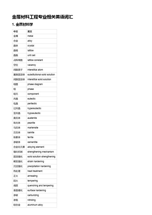
金属材料工程专业相关英语词汇1. 金属材料学中文英文金属metal合金alloy晶体crystal晶格lattice晶胞unit cell点阵常数lattice constant空位vacancy间隙原子interstitial atom置换固溶体substitutional solid solution间隙固溶体interstitial solid solution相图phase diagram相phase组元component共晶eutectic包晶peritectic过共晶hypereutectic亚共晶hypoeutectic奥氏体austenite珠光体pearlite马氏体martensite贝氏体bainite铁素体ferrite渗碳体cementite合金化元素alloying element强化机制strengthening mechanism固溶强化solid solution strengthening畸变强化strain hardening沉淀强化precipitation hardening热处理heat treatment正火annealing回火tempering调质quenching and tempering表面硬化surface hardening渗碳carburizing渗氮nitriding铝合金aluminum alloy中文英文铜合金copper alloy镁合金magnesium alloy钛合金titanium alloy2. 材料力学中文英文应力stress应变strain弹性模量elastic modulus, Young's modulus, modulus of elasticity 泊松比Poisson's ratio屈服强度yield strength抗拉强度tensile strength断裂韧性fracture toughness蠕变creep疲劳fatigue应力集中系数stress concentration factor应力强度因子stress intensity factor裂纹尖端crack tip裂纹扩展crack propagation裂纹扩展速率crack growth rate塑性变形plastic deformation弹性变形elastic deformation滞弹性变形anelastic deformation粘弹性变形viscoelastic deformation滑移slip滑移面slip plane滑移方向slip direction柏氏矢量Burgers vector位错dislocation索氏体spheroidite索氏化spheroidization3. 材料物理中文英文电子结构electronic structure能带理论band theory半导体semiconductor禁带宽度band gap本征半导体intrinsic semiconductor掺杂半导体doped semiconductor非平衡载流子excess carrierPN结PN junction二极管diode晶体管transistor集成电路integrated circuit磁性材料magnetic material磁化强度magnetization磁畴magnetic domain矫顽力coercivity饱和磁化强度saturation magnetization铁磁性ferromagnetism反铁磁性antiferromagnetism顺磁性paramagnetism抗磁性diamagnetism铁电材料ferroelectric material自发极化强度spontaneous polarization矫顽电场强度coercive electric field压电效应piezoelectric effect光学材料optical material折射率refractive index反射率reflectance透射率transmittance吸收系数absorption coefficient发光效应luminescence effect荧光材料fluorescent material发光二极管(LED)light-emitting diode (LED)激光器(LD)laser diode (LD)4. 材料热力学中文英文热力学thermodynamics系统system环境surroundings状态state过程process平衡equilibrium状态方程equation of state热力学第一定律first law of thermodynamics热力学第二定律second law of thermodynamics 熵entropy焓enthalpy自由能free energy吉布斯自由能Gibbs free energy海姆霍兹自由能Helmholtz free energy化学势chemical potential活度activity活度系数activity coefficient相律phase rule吉布斯相图Gibbs phase diagram杠杆规则lever rule相变phase transition相变焓变enthalpy change of phase transition相变熵变entropy change of phase transition相变自由能变free energy change of phase transition材料反应material reaction反应焓变enthalpy change of reaction反应熵变entropy change of reaction反应自由能变free energy change of reaction5. 材料测试中文英文金相组织观察metallographic observation 金相显微镜metallographic microscope 抛光机polishing machine腐蚀剂etchant晶粒度grain size显微硬度测试仪(Microhardness tester)microhardness tester维氏硬度(Vickers hardness)Vickers hardness布氏硬度(Brinell hardness)Brinell hardness洛氏硬度(Rockwell hardness)Rockwell hardness拉伸试验(tensile test)tensile test拉伸试验机(tensile testing machine)tensile testing machine标准试样(standard specimen)standard specimen应力-应变曲线(stress-strain curve)stress-strain curve弹性模量(elastic modulus)elastic modulus屈服点(yield point)yield point抗拉强度(tensile strength)tensile strength断后伸长率(elongation at break)elongation at break断面收缩率(reduction of area)reduction of area6. 材料分析中文英文光谱分析spectroscopy原子发射光谱atomic emission spectroscopy原子吸收光谱atomic absorption spectroscopy紫外-可见光谱ultraviolet-visible spectroscopy红外光谱infrared spectroscopy拉曼光谱Raman spectroscopy质谱分析mass spectrometry电感耦合等离子体质谱inductively coupled plasma mass spectrometry 二次离子质谱secondary ion mass spectrometry色谱分析chromatography气相色谱gas chromatography液相色谱liquid chromatographyX射线衍射X-ray diffraction布拉格方程Bragg's lawX射线荧光分析X-ray fluorescence analysis电子显微镜electron microscope扫描电子显微镜(SEM)scanning electron microscope (SEM)透射电子显微镜(TEM)transmission electron microscope (TEM)能量色散X射线能谱(EDS)energy dispersive X-ray spectroscopy (EDS)电子能量损失能谱(EELS)electron energy loss spectroscopy (EELS)7. 材料加工中文英文铸造casting模具mold浇注pouring凝固solidification缩孔shrinkage cavity缩松shrinkage porosity砂型铸造sand casting金属型铸造metal mold casting精密铸造precision casting锻造forging热锻hot forging冷锻cold forging自由锻open die forging模锻closed die forging轧制rolling热轧hot rolling冷轧cold rolling平板轧机flat rolling mill形状轧机shape rolling mill拉拔drawing拉丝机wire drawing machine挤压extrusion直接挤压direct extrusion间接挤压indirect extrusion8. 材料表征中文英文电学性能electrical property电阻率resistivity电导率conductivity电容capacitance介电常数dielectric constant电极化polarization耐压强度breakdown strength磁学性能magnetic property磁化曲线magnetization curve磁滞回线hysteresis loop矫顽力coercivity剩余磁化强度remanence磁导率permeability磁阻率reluctivity光学性能optical property折射率refractive index反射率reflectance透射率transmittance吸收系数absorption coefficient发光效应luminescence effect荧光材料fluorescent material9. 材料设计中文英文材料选择material selection材料性能指数material performance index材料选择图material selection chart材料性能预测material property prediction本构关系constitutive relation有限元分析finite element analysis材料组合优化material combination optimization复合材料composite material多层板sandwich panel功能梯度材料functionally graded material材料失效分析material failure analysis应力集中stress concentration裂纹扩展crack propagation脆性断裂brittle fracture韧性断裂ductile fracture疲劳断裂fatigue fracture蠕变断裂creep fracture10. 材料科学前沿中文英文纳米材料nanomaterial纳米粒子nanoparticle纳米线nanowire纳米管nanotube石墨烯graphene全息石墨烯holographic graphene生物材料biomaterial生物相容性biocompatibility生物降解性biodegradability组织工程tissue engineering药物传递drug delivery智能材料smart material形状记忆合金shape memory alloy磁致伸缩合金magnetostrictive alloy压电材料piezoelectric material电致变色材料electrochromic material超弹性合金superelastic alloy超导材料superconducting material能源材料energy material太阳能电池solar cell燃料电池fuel cell锂离子电池lithium-ion battery钠离子电池sodium-ion battery环境材料environmental material环境友好型材料eco-friendly material环境降解型材料environmentally degradable material 环境适应型材料environmentally adaptive material光催化材料photocatalytic material二氧化钛titanium dioxide水净化材料water purification material空气净化材料air purification material重金属吸附材料heavy metal adsorption material。
多层密度界面的拟BP神经网络反演方法

多层密度界面的拟BP神经网络反演方法刘展1赵文举2相鹏1(1.中国石油大学(华东)地球资源与信息学院,东营,257061 (2.东方地球物理勘探有限责任公司综合物化探事业部,涿州,072751)摘要提出一种根据重力异常反演三维密度界面分布的反演模式。
该模式将拟BP神经网络与重力反演理论结合,与传统神经网络不同的是拟BP神经网络不需要进行训练,而是直接求取隐层中的物性值。
该模式应用于合成数据集可以发现三维密度界面能够被很好的复原。
最后,利用该方法反演了冲绳海槽南部第三系底与莫霍面深度。
关键词三维重力反演,密度界面,拟BP神经网络,冲绳海槽南,莫霍面,第三系基底1、引言根据重力异常求取三维密度界面的几何形态是重力数据解释工作的一个主要目标。
目前存在很多种不同的算法,例如,Oldenburg(1974)对Parker(1973)提出的非均匀层状介质正演公式重新推导得到根据已知重力异常求取密度界面深度的反演公式。
Rao等(1999)利用邻接直立棱柱体模型根据重力异常或者基底构造求取三维密度界面深度。
人工神经网络已经被成功地应用于地球物理数据处理和反演问题当中。
例如,测井数据解释(Wiener等,1991;Huang等1996),反射地震数据处理(Ashida,1996),近地表电磁成像模式识别(Poulton等,1992),密度界面反演(Taylor,Vasco,1991;朱自强,1995)等。
尽管取得了进步,但是众所周知的是神经网络的反演结果很大程度上取决于训练数据,所以训练数据的选择是决定神经网络性能的关键。
当训练数据与观测数据的模式存在很大差异时,神经网络会求出不合理的结果。
管志宁(1998)将BP神经网络与重磁异常反演相结合提出了一种新的反演算法—拟BP神经网络。
隐层中的物性值可以直接求出而不需要传统神经网络的训练过程。
本文提出一种迭代拟BP神经网络三维密度界面反演算法。
首先,简要回顾一下三维密度界面的正演模型;然后详细介绍拟BP神经网络三维密度界面反演算法;接着利用合成数据分析算法的性能;最后用该方法求取南冲绳海槽盆地的第三系基底和莫霍面深度。
磁滞伸缩驱动器磁滞特性的Persiach模型建模

磁滞伸缩驱动器磁滞特性的Persiach模型建模冒鹏飞;王传礼;喻曹丰;钟长鸣【摘要】Giant magnetostrictive material (GMM) exists intrinsic magnetic hysteresis nonlinearity, large hysterisis error will happened when it is used for precision positioning, accurate mathematical model to describe the hysteresis nonlinearity seems very important in control the output accuracy of the giant magnetostrictive actuatort.%超磁致伸缩材料具有本征磁滞非线性,用于精密定位时具有较大的回程误差.为控制超磁致伸缩驱动器的输出位移精度,需要建立准确的数学模型来描述其磁滞非线性.基于经典的Preisach磁滞模型,通过对Preisach磁滞模型的离散化,建立了超磁致伸缩驱动器的Preisach磁滞数学模型;并进行了超磁致伸缩驱动器输出位移实验研究.实验结果表明:模型计算的结果和实验结果基本吻合,证明所建模型能够较好地反映实际情况.【期刊名称】《科学技术与工程》【年(卷),期】2017(017)009【总页数】4页(P149-152)【关键词】超磁致伸缩材料(GMM);磁滞非线性;Preisach磁滞模型;离散化【作者】冒鹏飞;王传礼;喻曹丰;钟长鸣【作者单位】安徽理工大学机械工程学院,淮南 232001;安徽理工大学机械工程学院,淮南 232001;安徽理工大学机械工程学院,淮南 232001;安徽理工大学机械工程学院,淮南 232001【正文语种】中文【中图分类】TB34超磁致伸缩材料(gaint magnetostrictive material,GMM)是铁磁性功能材料[1],具有磁致伸缩应变大、能量密度高、响应速度快、输出力大、磁机耦合系数大、居里温度高等优点[2],并且能够实现电磁能—机械能的可逆转化,被称作是21世纪战略性高科技材料[2,3]。
(凝聚态物理专业论文)Ising模型磁性质的理论研究
摘要
磁性是物质的基本属性之一,对物质磁性质及其机理的研究一直是凝聚态物 理中重要的研究课题之一。近年来,层状高温超导材料、磁性多层膜、人造磁性 超品格、有机聚合物磁性材料的制备技术和实验研究发展迅速,这些新材料表现 出了许多奇特的磁性质,具有广阔的应用前景,这极大地促进了新型磁性材料的 理论研究。作为描述固体磁性的Ising模型也受到了许多理论工作者的关注。
上世纪20年代,量子力学迅速发展起来,人们开始用量子力学来解释物质 磁性的起源。1928年,W.Heisenberg把铁磁物质的自发磁化归结为原子磁矩之 间的直接交换作用,建立了局域性电子自发磁化的Heisenberg交换作用理论模 型,从而正确地揭示了自发磁化的量子本质。这一理论不但成功地解释了物质存 在铁磁性、反铁磁性和亚铁磁性等实验事实,而且为进一步导出低温自旋波理论、 铁磁相变理论及铁磁共振理论奠定了基础。
H=忑∑氓1%,slisU+JlH秣㈨islis㈨+“.蠢tt乳IsliSⅧ、)
I(,.』)Leabharlann 我们用相关有效场理论对系统的磁性质进行了研究,推导出了系统磁矩和 相变温度的表达式。研究了温度、交换相互作用常数和稀磁浓度对各层原子磁矩 和相变温度的影响,还给出了磁矩随原子层数的变化规律。研究结果表明,对自 旋值较小的原子层来说,层间交换相互作用比层内交换相互作用对该层磁矩的影 响大得多,这直接导致低自旋材料在界面处出现磁矩最大值,而高自旋材料在界 面处出现磁矩最小值。我们还发现,稀磁情况下磁矩随温度的变化趋势与未稀磁 时类似,不同的是磁矩大小相应减小。
expressed as
H=一∑∑(‘。,S,,甄+以tf+。S,,S…,,+‘,『_。S,,S,..,,) , (,,』)
The effective field theory、析t11 correlations based on Ising model is discussed in detail.We investigate the magnetization,critical temperature and compensation
Journal of Alloys and Compounds 448(2008)73-76 The

Journal of Alloys and Compounds448(2008)73–76The magnetic entropy change in CoMnSballoys with different crystal sizesShandong Li a,b,∗a Department of Physics,Fujian Normal University,Fuzhou350007,Chinab National Laboratory of Solid State Microstructure and Department of Physics,Nanjing University,Nanjing210093,ChinaReceived30November2006;received in revised form11March2007;accepted12March2007Available online16March2007AbstractThe magnetocaloric effect(MCE)in CoMnSb has been investigated by comparing two samples with different crystal size.One sample is the ingot with crystal size of120nm,referred as sample A.The other with average crystal size of30nm has been fabricated by rapid solidification method,referred as sample B.It has been found that crystal size dramatically affects the magnetic properties and MCE for CoMnSb alloy.For example,in comparison with sample A,sample B exhibits a lower magnetization and Curie temperature,but an enhanced refrigerant capacity and broader working temperature range.These facts indicate that sample B is superior to the ingot in practical application.The above results are explained in terms of the effect of crystal size and atomic disorder on the intrinsic magnetic properties and magnetic entropy change.©2007Elsevier B.V.All rights reserved.Keywords:Nanostructured materials;Magnetocaloric;Transition metals alloys and compounds1.IntroductionIn recent years,the magnetic refrigerants have drawn an increasing attention because they are more protective towards our living environment than the conventional vapor-cycle refrig-erant[1,2].In comparison with gas refrigerators,magnetic refrigerators have a number of advantages,such as high effi-ciency,small volume and ecological cleanliness.The magnetic refrigeration makes use of the cycles of magnetization and demagnetization of a magnetic material,so that the develop-ment of new materials with a giant MCE is strongly desired. The research for materials with large magnetocaloric effect is being continued since the discovery of MCE in iron by Warburg about100years ago[1].Some magnetic materials with afirst-order or second-order transition have attracted much attention, since they have large MCE[2–6].∗Correspondence address:Department of Physics,Fujian Normal University, Fuzhou350007,China.Tel.:+8659183486160;fax:+86-591-83465313.E-mail address:dylsd007@.It is known that above15K,Ericsson cycle is used in magneticrefrigeration in order to remove the effect of the lattice entropy[7].Thermodynamic analysis shows that efficient operation ofan ideal Ericsson cycle requires a constant-induced magneticentropy change as a function of temperature over the requiredoperating range[8].If a magnetic working material has a largemagnetic entropy change(| S M|)peak at the transition tem-perature,but falls off rapidly on either side,it is not suitablefor use in devices utilizing the Ericsson cycle[3].Therefore,it is significant to explore a magnetocaloric material with highMCE and wide operating temperature span and/or to widen theoperating temperature span for the high MCE material by useof some novel methods.It was reported that nanoparticles fab-ricated by rapid solidification or chemical method,may haverelatively wider working temperature span[9].In our previous work,the MCE of CoMnSb alloy has beenreported as an exploration for useful MCE materials[10].Dueto the large Mn magnetic moments,this kind of rare-earth-freealloy may be a potential candidate of large MCE materi-als.In order to extend the operating temperature span and toenhance the refrigerant capacity of CoMnSb alloy,the nanocrys-talline CoMnSb alloy has been fabricated by rapid solidification0925-8388/$–see front matter©2007Elsevier B.V.All rights reserved. doi:10.1016/j.jallcom.2007.03.05274S.Li/Journal of Alloys and Compounds448(2008)73–76 method.In this paper,the effect of crystal size and atomic dis-order on the MCE of CoMnSb alloy have been investigated bycomparing the MCE of two samples with different crystal sizes.2.Experimental procedureTwo types of CoMnSb alloys with different crystal sizes have been preparedby an induction-melting and a melt-spinning method,respectively.The highpurity metals of Co,Mn and Sb were melted in an induction melting furnacefor three times under Ar atmosphere.Then,the ingot was sealed in a quartztube under vacuum atmosphere(less than3×10−3Pa).The sealed ingot wasannealed at873K for30h for eliminating inner stress.The annealed samplewith large crystal size was referred to as sample A,while the other sample withsmall crystal size,fabricated by melt-spun part of the ingot at a circumferencespeed of30m/s in vacuum,was referred to as sample B.The magnetic properties of the samples were measured by using vibratingsample magnetometer(VSM)and superconducting quantum interference device(SQUID)magnetometer.The microstructure of the materials was characterizedby an X-ray diffractometer(XRD)with Cu K␣radiation.3.Results and discussionFig.1shows the XRD curves for the samples A and B.Theindexes of CoMnSb facets were signed in Fig.1.As illustrated,both samples are composed of a single phase of CoMnSb.It canalso be seen that the diffraction peaks of sample A are greatsharper than those of sample B,indicating that the crystal sizeof sample A is great coarser than that of sample B.The crystalsizes of samples A and B,calculated by Scherrer equation,areabout120and30nm,respectively.The temperature dependence of magnetization for both sam-ples was measured by VSM in the magneticfield of0.2T.Fig.2shows the M–T relationship curves for samples A and B.It can beseen that:(1)the transition temperature of sample B is slightlylower than that of sample A.The Curie temperatures are471and468K for samples A and B,respectively,and(2)the mag-netization of sample B is slightly lower than that of sample A attemperature range less than T C.Fig.3shows a series of magnetization isotherms measured atdifferent temperatures in the vicinity of Curie temperature,T C,with the maximum appliedfield of0.9T.The magnetic entropychange,| S M|,was determined as a function of temperatureandFig.1.The XRD traces for samples A andB.Fig.2.The temperature dependence of magnetization for samples A and B.magneticfield from isothermal magnetization curves by use ofMaxwell equation:S M=H2H1∂M(H,T)∂THd H(1)Fig.4shows the plots of| S M|versus temperature of sam-ples A and B for the magneticfield changing from0to0.9T,respectively.Although,the maximum value of| S M|for sampleB(1.32J/kg K)is smaller than that for sample A(2.06J/kg K),a broader peak for sample B is observed in the| S M|–T curves,indicating that sample B may be superior to the bulk materialfor practical application in Ericsson cycle.In practice,how much heat can be transferred between the cold and hot sinks in one ideal refrigeration cycle is characterizedby the refrigerant capacity[11].The refrigerant capacity,q,isdefined asq=ThotT coldS(T,P, H)P, H d T(2)Fig.3.The magnetization isotherms measured at different temperatures near T Cfor samples A and B.S.Li/Journal of Alloys and Compounds448(2008)73–7675Fig.4.The plots of| S M|vs.temperature for samples A and B with H=0.9T. where T cold and T hot are the temperature of the cold and hotsinks,respectively.Therefore,when two different materials areused in the same refrigeration device,the material with higherrefrigerant capacity is expected to perform better,since it willsupport transport of greater amounts of heat in a real cycle,provided all parameters of a magnetic refrigerator remain thesame.From Fig.4,it can be seen that the optimum operatingtemperature range of sample B is wider than that of sample A.Inorder to accurately evaluate the refrigerant capacity for materialswith different peak site and operating temperature span,we takethe temperature range between the full-width at half maximumas the calculating temperature span in Eq.(2).The temperaturespans for samples A and B are466–475and452.3–477.4K,respectively.For the magneticfield changing from0to0.9T,therefrigerant capacities for samples A and B are15.3and27.3J/kg,respectively,according to Eq.(2).In addition,even taking thesame temperature span of433–483K,the refrigerant capacityof sample B(42.83J/kg)is slightly larger than that of sampleA(41.28J/kg).Consequently,sample B is superior to sample Ain practical paring with sample A,the smoothpeak of magnetic entropy change and larger refrigerant capacityof sample B indicate that sample B is a preferential choice ratherthan sample A.It is believed that magnetic properties of CoMnSb alloy withcrystal size of120nm can be considered as the bulk ones.The saturation magnetization(M s)of sample A was measuredby SQUID at3T and2K.If,approximately,taking the M sof94.2533emu/g at2K as the real saturation magnetizationM s(0)of CoMnSb alloy,the calculated saturation magnetiza-tion is3.978B/f.u.for sample A.This value is very close tothe theoretical and experimental result of M s∼4.0B/f.u.for CoMnSb alloy[12].While the crystal size is decreasing to smallsize(e.g.30nm),the magnetic exchange interaction and mag-netic anisotropy deviate from the bulk material,giving rise to aslight reduction of the magnetization and T C[13,14].This phe-nomenon was widely observed in nanocrystalline ferromagneticsystems[15,16].Moreover,the effect of crystal size distributionon the inner magnetic properties(e.g.the saturation magnetiza-tion,T C)for nanocrystallite materials is great larger than that forbulk one[17].With raising temperature,the nanocrystallite fer-romagnetic material transforms to the paramagnetic state priorto the bulk one.As a result,a relatively lower transition tem-perature in M–T curve for nanocrystalline materials than thatfor bulk ones is expected.In addition to that,the distributionof crystal size for the nano-ferromagnetic materials also givesrise to afluctuation of T C accordingly.Therefore,the broaden-ing of| S M|peak and enhancement of refrigerant capacity in sample B in comparison with sample A can be,at least partially,attributed to the broad T C distribution induced by small size andits distribution.Atomic disorder generally occurs in half-Heusler alloys,suchas CoMnSb and NiMnSb[18,19].In our previous work[20],theatomic disorder of CoMnSb alloys was reduced by annealing thesample at1323K for50h.A superstructure with low atomic dis-order was formed for the sample annealed at high temperature.The broadening of operating temperature span and the enhance-ment of refrigerant capacity can be attributed to the formationof the superstructure.Ref.[20]implies that the atomic disorderin CoMnSb alloy deteriorates the MCE.In this study,sampleA was annealed at873K for30h for the aims of eliminatinginner stress and reducing the atomic disorder.Sample B was notannealed for avoiding the grain growth.It is well known that theatomic disorder is stronger for the sample prepared by quench-ing than the ingot.This can also be demonstrated by the XRDresults.The diffraction peaks of sample B are slightly shiftedto left side in comparison with those of sample A,suggestinga relatively larger atomic disorder in quenched sample B thanin sample A.Therefore,the measured refrigerant capacity islower than the real value due to the stronger atomic disorder insample B.In other words,the effect of crystal size on MCE ispartially reduced by atomic disorder for the quenched sample.The improvement of MCE in sample B is dominated by crystalsize effect.4.ConclusionThe magnetic properties and magnetocaloric effect ofCoMnSb alloys with different crystal sizes have been investi-paring to the sample with crystal size larger than100nm,the refrigerant capacity is enhanced and the operatingtemperature span is extended for the sample with crystal size assmall as several tens of nanometer.These results suggest thatCoMnSb alloy with small crystal size is superior to the largerone in practical application.AcknowledgementsThis work wasfinancially supported by National ScienceFoundation of China(NSFC)for Young Scientists(Grant No.:10504010),Key Project of Fujian Provincial Department of Sci-ence&Technology(2006H0018)and Science Foundation ofFujian Province of China(2006J0152and2005J023). References[1]E.Warburg,Ann.Phys.(Leipzig)13(1881)141.[2]V.K.Pecharsky,K.A.Gschneidner Jr.,Phys.Rev.Lett.78(1997)4494.76S.Li/Journal of Alloys and Compounds448(2008)73–76[3]B.J.Korte,V.K.Pecharsky,K.A.Gschneidner Jr.,J.Appl.Phys.10(1998)5677.[4]F.W.Wang,X.X.Zhang,F.X.Hu,Appl.Phys.Lett.77(2000)1360.[5]O.Tegus,E.B¨u rck,K.H.J.Buschow,F.R.de Boer,Nature415(2002)150.[6]S.D.Li,M.M.Liu,Z.R.Yuan,L.Y.L¨u,Z.C.Zhang,Y.B.Lin,Y.W.Du,J.Alloys Compd.427(2007)15.[7]T.Hashimoto,T.Kuzuhara,M.Sahashi,K.Inomata,A.Tomokiyo,H.Yayama,J.Appl.Phys.62(1987)3873.[8]A.Smaili,R.Chahine,J.Appl.Phys.81(1997)824.[9]D.H.Wang,S.L.Tang,H.D.Liu,S.D.Li,J.R.Zhang,Y.W.Du,Jpn.J.Appl.Phys.40(2001)6815.[10]S.D.Li,M.M.Liu,Z.G.Huang,F.Xu,W.Q.Zou,F.M.Zhang,Y.W.Du,J.Appl.Phys.99(2006)063901.[11]V.P.Pecharsky,K.A.Gschneidner Jr.,J.Appl.Phys.90(2001)4614.[12]V.Ksenofontov,G.Melnyk,M.Wojcik,S.Wurmehl,K.Kroth,S.Reiman,P.Blaha,C.Felser,Phys.Rev.B74(2006)134426.[13]R.H.Kodama,S.H.Makhlouf,A.E.Berkowitz,Phys.Rev.Lett.79(1997)1393.[14]J.M.D.Coey,Phys.Rev.Lett.27(1971)1140.[15]T.Sato,T.Iijima,M.Seki,N.Inagaki,J.Magn.Magn.Mater.65(1987)252.[16]J.F.L¨o ffler,J.P.Meier,B.Doudin,J.P.Ansermet,W.Wagner,Phys.Rev.B57(1998)2915.[17]R.H.Kodama,J.Magn.Magn.Mater.200(1999)359.[18]C.PalmstrØm,MRS Bull.(October)(2003)725.[19]K.Kaczmarska,J.Pierre,J.Tobola,R.V.Skolozdra,Phys.Rev.B60(1999)373.[20]S.D.Li,Z.R.Yuan,L.Y.L¨u,M.M.Liu,Z.G.Huang,F.M.Zhang,Y.W.Du,Mater.Sci.Eng.A428(2006)332.。
yig金属异质结构中自旋泵浦效应的研究
YIG/金属异质结构中自旋泵浦效应的研究摘要自旋流是材料内部自旋角动量的定向输运。
它既是自旋电子学中新物理效应出现的核心自由度,又是构建新一代高密度、高速度、低能耗磁性存储与处理器件中实现局域自旋(或磁矩)翻转的核心载体。
掌握自旋流的物理特性以及自旋流与材料相互作用的微观机制,已成为理解自旋与电荷和轨道多自由度耦合以及推动纯自旋流应用的关键科学问题。
本论文围绕以上关键科学问题,以钇铁石榴石/金属(YIG/NM)异质结构中的自旋泵浦效应为主要研究手段,开展了纯自旋流物理特征、有效自旋混合电导率(表征纯自旋流注入效率)、以及自旋霍尔角(表征自旋流与电荷流转化效率)三个方面的研究。
取得的主要创新性结论如下:1、 提出了获得纯自旋泵浦信号的方法,并建立了纯自旋流的空间对称性。
我们针对FM/NM 中可能同时存在自旋整流和自旋泵浦信号的问题,提出了利用YIG/NM 体系,实现纯自旋泵浦信号的测量。
发现磁化强度在xy 、yz 、xz 平面转动时,自旋泵浦和自旋整流信号的角度依赖关系明显不同。
同时,还发现了满足3cos θ角度关系的非均匀自旋泵浦信号。
因此,自旋泵浦信号的准确测量需要利用空间对称性排除自旋整流影响,在=90θ 或Hall 端进行测量。
2、 实现了1Pt Pd x x −(01x ≤≤)合金自旋霍尔角的准确表征,并提出了1Pt Pd x x −合金自旋霍尔角的主要微观机制。
通过标定自旋扩散长度、有效混合电导率、以及微波磁场大小,利用=90θ 几何下测量的YIG/1Pt Pd x x −自旋泵浦信号,确定了1Pt Pd x x −合金的自旋霍尔角(Pt =0.1250.015SH θ±)。
利用自旋霍尔角与电荷电导率的标度关系,通过自旋霍尔角随x 的变化,揭示了斜散射是1Pt Pd x x −中自旋相关散射的主要微观机制。
3、 提出了有效自旋混合电导率与磁化强度进动的关系,实现了有效混合电导率的调控。
ASTM材料与实验标准.A977A977M
Designation:A977/A977M–02Standard Test Method forMagnetic Properties of High-Coercivity Permanent Magnet Materials Using Hysteresigraphs1This standard is issued under thefixed designation A977/A977M;the number immediately following the designation indicates the year of original adoption or,in the case of revision,the year of last revision.A number in parentheses indicates the year of last reapproval.A superscript epsilon(e)indicates an editorial change since the last revision or reapproval.1.Scope1.1This test method describes how to determine the mag-netic characteristics of magnetically hard materials(permanent magnets),particularly their initial magnetization,demagneti-zation,and recoil curves and such quantities as the residual induction,coercivefields,kneefield,energy products,and recoil permeability.This test method is suitable for all materi-als processed into bulk magnets by any common fabrication technique(casting,sintering,rolling,molding,and so forth), but not for thinfilms or for magnets that are very small or of unusual shape.Uniformity of composition,structure,and properties throughout the magnet volume is necessary to obtain repeatable results.Particular attention is paid to the problems posed by modern materials combining very high coercivity with high saturation induction,such as the rare-earth magnets, for which older test methods(see Test Method A341)are unsuitable.An applicable international standard is IEC Publi-cation404-5.1.2The magnetic system(circuit)in a device or machine generally comprisesflux-conducting and nonmagnetic struc-tural members with air gaps in addition to the permanent magnet.The system behavior depends on properties and geometry of all these components and on the temperature.The tests described here measure only the properties of the perma-nent magnet material.The basic test method incorporates the magnetic specimen in a magnetic circuit with a closedflux path.Test methods using ring samples or frames composed entirely of the magnetic material to be characterized,as commonly used for magnetically soft materials,are not appli-cable to permanent magnets.1.3This test method shall be used in conjunction with Practice A34/A34M.1.4The values and equations stated in customary(cgs-emu or inch-pound)or SI units are to be regarded separately as standard.Within this test method,SI units are shown in brackets except for the sections concerning calculations where there are separate sections for the respective unit systems.The values stated in each system may not be exact equivalents; therefore,each system shall be used independently of the other. Combining values from the two systems may result in noncon-formance with this test method.1.5The names and symbols of magnetic quantities used in this test method,summarized in Table1,are those currently preferred by U.S.industry.1.6This test method is useful for magnet materials havingH ci values between about100Oe and35kOe[8kA/m and2.8 MA/m],and B r values in the approximate range from500G to 20kG[50mT to2T].High-coercivity rare-earth magnet test specimens may require much higher magnetizingfields than iron-core electromagnets can produce.Such samples must be premagnetized externally and transferred into the measuring yoke.Typical values of the magnetizingfields,H mag,required for saturating magnet materials are shown in Table1.1.7This standard does not purport to address all of the safety concerns,if any,associated with its use.It is the responsibility of the user of this standard to establish appro-priate safety and health practices and determine the applica-bility of regulatory limitations prior to use.2.Referenced Documents2.1ASTM Standards:A34/A34M Practice for Procurement Testing and Sam-pling of Magnetic Materials2A340Terminology of Symbols and Definitions Relating to Magnetic Testing2A341/A341M Test Method for Direct Current Magnetic Properties Using dc Permeameters and the Ballistic Test Methods2E177Practice for Use of the Terms Precision and Bias in ASTM Test Methods32.2Magnetic Materials Procedure Association Standard: MMPA No.0100–96Standard Specifications for Perma-nent Magnet Materials41This test method is under the jurisdiction of ASTM Committee A06onMagnetic Properties and is the direct responsibility of Subcommittee A06.01on Test Methods.Current edition approved Oct.10,2002.Published November2002.Originally published as A977–st previous edition A977–97.2Annual Book of ASTM Standards,V ol03.04.3Annual Book of ASTM Standards,V ol14.02.4Available from Magnetic Materials Producers Association,8S.Michigan Ave., Suite1000,Chicago,IL60603.1Copyright©ASTM International,100Barr Harbor Drive,PO Box C700,West Conshohocken,PA19428-2959,United States.2.3International Electrotechnical Commission Document:Publication 404-5Magnetic Materials –Part 5:Permanent Magnet (Magnetically Hard)Materials –Methods of Measurement of Magnetic Properties 53.Terminology3.1Basic magnetic units are defined in Terminology A 340and MMPA Standard No.0100–96.Additional definitions with symbols and units are given in Table 1and Figs.1-3of this test method.4.Significance and Use4.1This test method is suitable for magnet specification,acceptance,service evaluation,quality control in magnet production,research and development,and design.4.2When a test specimen is cut or fabricated from a larger magnet,the magnetic properties measured on it are not necessarily exactly those of the original sample,even if the material is in the same condition.In such instances,the test results must be viewed in context of part performance history.4.3Tests performed in general conformity to this test method and even on the same specimen,but using different test systems,may not yield identical results.The main source of discrepancies are variations between the different test systems in the geometry of the region surrounding the sample,such as,size and shape of the electromagnet pole caps (see Annex A1and Appendix X1),air gaps at the specimen end faces,and especially the size and location of the measuring devices for H and B or for their corresponding flux values (Hall-effect probes,inductive sensing coils).Also important is the methodof B calibration,for example,a volt-second calibration of the fluxmeter alone versus an overall system calibration using a physical reference sample.The method of B and H sensing should be indicated in test reports (see Section 9).5.Measuring Methods and Apparatus5.1Measuring Flux and Induction (Flux Density):5.1.1In the preferred B -measuring method,the total flux is measured with a sensing coil (search coil)that surrounds the test specimen and is wound as closely as possible to the specimen surface.Its winding length should be no more than a third of the specimen length,preferably less than one fifth,and must be centered on the specimen.The leads shall be twisted tightly.As the flux changes in response to sweeping the applied field,H ,the total flux is measured by taking the time integral of the voltage induced in this coil.This measurement is taken with a fluxmeter.Modern hysteresigraphs use electronic inte-grating fluxmeters that allow convenient continuous integra-tion and direct graphic recording of magnetization curves.If the signal is large enough,high-speed voltage sampling at the coil and digital integration is also possible.5.1.2The magnetic induction,B ,is determined by dividing the total flux by the area-turns product,NA ,of the B -sensing coil.For permanent magnets in general,and especially for high-coercivity materials,an air-flux correction is required (see 5.3and 5.4).5.1.3The total error of measuring B shall be not greater than 62%.5.1.4The change of magnetic induction,D B =B 2–B 1,in the time interval between the times t 1and t 2is given as follows:D B 5~108/AN !*t 1t 2e dt ~customary units !(1)D B 5~1/AN !*t 1t 2e dt ~SI units !(2)where:B =magnetic induction,G [T];A =cross-sectional area of the test specimen,cm 2[m 2];N =number of turns on the B -sensing coil;e =voltage induced in the coil,V;t=time,s;and*t 1t 2e dt=voltage integral =flux,V-s [Weber].5.1.5The change in the magnetic induction shall be cor-rected to take into account the air flux outside the test specimen that is linked by the sensing coil.The corrected change,B corr ,is given as follows:D B corr 5~108/AN !*t 1t 2e dt 2D H ~A t 2A !/A ~customary units !(3)D B corr 5~1/AN !*t 1t 2e dt 2µ0D H ~A t –A !/A ~SI units !(4)where:A =average cross-sectional area of the sensing coil,cm 2[m 2];D H =change in field from t 1until t 2,Oe [A/m];and µ0=magnetic constant [4p 10-7H/m].5.2Determining Intrinsic Induction :5Available from International Electrotechnical Commission (IEC),3rue de Varembé,P.O.Box 131,CH-1211,Geneva 20,Switzerland.TABLE 1Symbols,Quantities,and UnitsN OTE 1—IEC nomenclature calls B r “remanence,”when B r represents the B at H =0of the outermost hysteresis loop,and it calls B r “remanent magnetic induction”for B at H =0at smaller loops.SymbolQuantitySI Unit Customary cgs-emuA t Cross section of search coil [m 2]cm 2B d Magnetic induction at BH max[T]G B rec Magnetic induction at low point of recoil loop[T]GB r Magnetic induction at remanence [T]G d l Diameter of pole piece[m]cm d 2Diameter of homogeneous field [m]cm H d Magnetic field strength at BH max [A/m]Oe H p Magnetic field strength at low point ofrecoil loop[A/m]Oel Distance between pole faces [m]cm l r Length of test sample[m]cm N Number of turns of test coil e Voltage induced in test coil V V dTotal air gap between test sample and pole faces[m]cmµ0A constant with value µ0=4p 10-7H/mµrecRecoilpermability5.2.1For high-coercivity magnets,it is more convenient to sense directly an electrical signal proportional to the intrinsic induction,derive the average B i by dividing this flux by the area-turns product of the surrounding B coil,and to plot B i versus H as the primary demagnetization curve.B then is obtained by mathematical or electronic addition of H to B .5.2.2The change of intrinsic induction in the test specimen can be determined by integrating the voltage induced in a device comprising two sensing coils,both subject to the same applied field H ,where the test specimen is contained in only one of the coils (Coil 1).If each individual coil has the same area-turns product,and if the windings are connected electri-cally in opposition,the signal induced by the flux linking Coil 2(not containing the specimen)will compensate for the output of Coil 1except for B i within the test specimen.The change of intrinsic induction in the specimen then is given as follows:D B i 5~108/AN !*t 1t 2e dt ~customary units !(5)FIG.1Normal and Intrinsic Hysteresis Loops and Initial Magnetization Curves for Permanent Magnet Materials Illustrating TwoExtremes of Virgin SampleBehaviorFIG.2Normal and Intrinsic Demagnetization Curves with Symbols for Special Points of Interest and Definition of Salient Properties.Illustration of Maximum Energy Product,CoerciveFields,and Definition of KneeFieldD B i 5~1/AN !*t 1t 2e dt ~SI units !(6)where:B i =intrinsic induction,G [T];A =cross section of the test specimen,cm 2[m 2];and N =number of turns on Coil 1containing the test speci-men.5.2.3The two-sensing-coil device shall lie totally within the homogeneous field defined by Eq A1.1and Eq A1.2.Test specimens of lower-coercivity magnets having a range of cross-sectional areas and shapes can then be measured with the same coil device.An arrangement of side-by-side coils of equal size is useful.Serious errors,however,are incurred when measuring B i this way on high-B r or high/coercivity magnets,or both,at applied fields of about 10kOe or more.The errors are most severe for test specimens of short pole-to-pole length.Local pole-piece saturation causes strong field inhomogene-ities.The specimen then must fill the cross section of Coil 1,and Coil 2must be a thin and flat coil,or a coaxial annular coil,either centered on the specimen or in close proximity to its surface (see 5.3).5.2.4The total error of measuring B i shall be not greater than 62%.5.3Measuring the Magnetic Field Strength :5.3.1For correct magnetization curves,one should know the magnetic field strength,H ,inside the test specimen,averaged over the specimen volume if H is not uniform.But this inner field cannot be measured.At the surface of the test specimen,H is equal to the local field strength just inside the specimen in those locations (and only there)where the H vector is parallel to the side surface of the specimen.Therefore,a magnetic field strength sensor of small dimensions relative to the specimen is placed near the specimen surface and sym-metrical with respect to the end faces,covering the shortest possible center portion of the specimen length.It shall be so oriented that it correctly measures the tangential field compo-nent.5.3.2To determine the magnetic field strength,a flat surface coil,a tightly fitted annular coil,a magnetic potentiometer,or a Hall probe is used together with suitable instruments.The dimensions of the magnetic field sensor and its location shall be such that it is within an area of limited diameter around the test specimen (see Annex A1).5.3.3The provisions of 5.3.2are adequate for measure-ments on magnets having low-to-moderate intrinsic coercivity,such as Alnico and bonded ferrites.For high-coercivity,dense ferrites and especially for most rare earth-transition metal materials,it is essential for accurate measurement to use thin flat or radially thin annular H -sensing coils of short length (<1/5to 1/3of the specimen length),centered on the specimen and placed as close as possible to the specimen surface.5.3.4The same considerations apply to the H -flux compen-sation coil used in B i measurements (see 5.2.3.)When pole saturation can occur,Coil 2also shall be a thin conforming flat surface coil for rectangular specimen shapes or a thin annular coil closely surrounding a cyclindrical specimen,and the specimen essentially shall fill the open cross-sectional area of the B –sensing Coil 1.5.3.5To reduce other measurement errors,the air gaps between the flat ends of the test specimen and the pole pieces shall be kept small,typically in the range 0.001to 0.002in.[0.025to 0.050mm](see Fig.4).5.3.6The magnetic field strength measuring system shall be calibrated.Any temperature dependence of the measuring instruments,(for example,Hall probes),must be taken into account.The total error of measuring H shall be not greater than 62%.N OTE 1—The end faces of the test specimen should be in intimate contact with the pole faces.There are always unavoidable small air gaps as a result of surface roughness,poor parallelism of sample or pole faces,or intentional shimming to protect delicate specimens from deformation or crushing.These cause additional errors in the magnetic field strength measurement and indirectly in the B i measurements through air flux compensation errors,even in the low H region.The maximum error in the field strength measurement,as a result of two symmetric gaps of length d (see Fig.3)is approximately:D H/H 52B d /l r H ~customary units !(7)D H /H 52B d /µ0l r H ~SI units !(8)To keep the error 100D H /H <1%in the region of the (BH )max point,the gap thickness should be kept below the following values:d =0.00025l r for Alnicomagnets,FIG.3Normal and Intrinsic Demagnetization Curves with Symbols for Special Points of Interest and Definition of Salient Properties.Illustration of Recoil Loop.Recoil Permeability isDefined as µrec D B /DHFIG.4Illustration Regarding the Influence of Air Gaps at the EndFaces of the TestSpecimend=0.005l r for hard ferrite magnets,andd=0.003l r for rare-earth magnets.5.4Plotting Magnetization and Demagnetization Curves: 5.4.1Plotting of B i,H curves or B,H curves is accom-plished by combining one of the methods for magneticfield strength measurement from5.3with a B i-measuring method from5.2or a B-measuring method from5.1.A schematic for a typical hysteresigraph system is shown in Fig.5.5.4.2Continuous Plotting of Magnetization Curves—Modern electronic integrators used in conjunction with induc-tive sensors for B i or B,and in some instruments also for H, allow the continuous recording of magnetization,demagneti-zation,or recoil curves.A wide range offield sweep rates is possible.In the simplest but least desirable case,the exciting current of the electromagnet may be varied linearly,or thefield sweep rate may be held constant.Even better it may be controlled with feedback from the measuring circuit for the (intrinsic)induction so as to achieve an approximately constant rate of change of B i or B.Flexible sweep control requires a power supply for the electromagnet that can be programmed by an analog or digital electronic signal.For greatestflexibility, the power supply should be bipolar.Typical total recording times for a full hysteresis loop are between about30s and5 min.Integrator drift errors can be kept acceptably small with reasonable operator care.The output voltages of the integrators and a Hall-effectfield meter,if used,can be plotted directly with an analog x,y recorder,and salient property values are determined from this plot.Alternatively,the output voltages can be digitized,stored,and processed in a computer.Curves and calculated numerical values are then displayed on a monitor and printed out with a plotter or printer.6.Calibration6.1The subsystems of the hysteresigraph for measuring field andflux quantities must be calibrated from time to time. Several alternative techniques are in common use.All ensure comparable degrees of reproducibility,but they yield strongly different absolute accuracy.The circuits for measuringflux (induction or intrinsic induction)and the magnetizingfield are usually calibrated independently.However,checking hysteresi-graphs against each other by remeasuring demagnetization curves of reference magnets may link these two necessary calibrations.6.2Magnetic Flux and Induction:6.2.1Electronicfluxmeters are conveniently calibrated by using one of the following four methods.An accuracy of 60.1%is achievable by the methods listed in6.2.1.1-6.2.1.3. An error of65%must be expected from the method given in 6.2.1.4.All these methods,however,calibrate only the elec-tronic integrating and indicating/recording instrument.They leave out the hysteresigraph’s sensing coils,which introduce errors because of their location relative to test specimen and electromagnet pole caps,and whose area-turns product can change as the coils age or are abused.The specimen geometry itself also affects the B i calibration.Experience has shown discrepancies of5to10%between B i measurements on different hysteresigraphs calibrated with volt-second standards. The fourfluxmeter calibration methods are:6.2.1.1Use of a volt-second generator,consisting of a very stable source of a well-measured dc voltage and a precision timer.The level of this voltage and the length of time it is applied should be comparable to typical levels during a magnetic loop measurement with the hysteresigraph.6.2.1.2Use of a mutual inductance standard,by switching on and off a primary current measured with a precision ampere-meter.A knownflux change is induced in the second-ary winding of the standard,which serves as the V-s calibration signal in thefluxmeter circuit.6.2.1.3Use of a search coil of precisely known area-turns, that is moved into or removed from region of a time-constant homogeneousfield,which has been measured with a nuclear magnetic resonance(NMR)gaussmeter.A rigidly constructed magnetic circuit comprising a highly stable permanent magnet with large iron pole pieces and a short air gap is a suitablefield source for this.If it is well stabilized and shieldedfrom FIG.5Schematic Representation of a Typical Magnetic Hysteresigraph TestSystemmagnetic disturbances and physical abuse,it can continue to serve as a transfer standard after having once been calibrated by NMR.6.2.1.4Use of the remanent inductionflux,of a long, freestanding permanent magnet bar as a secondary standard.A close-fitting,short-search coil of exactly known turns count is placed in the center(neutral zone)of the much longer bar,the fluxmeter is zeroed and the coil removed to afield-free region of space.Alternatively,the coil can befixed and the magnet removed.The reference magnet should be precision machined from a material having a low temperature coefficient and high chemical andflux stability,such as Alnicofive or temperature compensated Sm,Gd-Co-based2-17magnets;it must be stabilized by magnetic and thermal cycling.Its average cross-sectional area must be known.6.2.2The preferred method for calibrating the entireflux-measuring subsystem(B i or B circuits,comprising the sensing coil arrangement,integrator,and indicating or recording instru-ment)uses a physical standard of a shape and size similar to that of the specimen to be characterized.Pure nickel is an excellent reference material since nickel is magnetically soft and thus easily saturated,its saturation magnetization value and temperature variation are well known,and nickel has a saturation induction level in the range of most permanent magnets.Pure iron is sometimes used,especially when cali-brating to measure only permanent magnets with the highest induction levels.Theflux calibration standard is placed in the air gap of the electromagnet,using the same pole and sensing-coil geometry to be used in the measurement for which one is calibrating.A magnetizingfield of the magnitude required to produce a known magnetization in the standard is applied,and using the sensitivity potentiometers of the integrator or re-corder,the y deflection on the x,y recorder is adjusted to yield a convenient scale factor for B i.The known magnetization at the appliedfield value,any temperature variation of this value, and the ratio of the cross-sectional areas of standard and test specimen must be taken into account.6.2.3For measurements on high-B,high-H ci materials,and specimens of short magnetic length,the relatively complex calibration method of6.2.2yields better accuracy for B i and B than the seemingly absolute,volt-second-basedfluxmeter cali-bration of 6.2.1.It takes into account most of the self-demagnetizing effects,field andflux inhomogeneities as a result of specimen shape and air gaps at sample end faces,and also pole-piece saturation effects,since many of these occur similarly with the nickel standard and the magnet test speci-men.Experience shows the error of B i in this case to be<2% in the appliedfield range up to about10to12kOe[800to1000 kA/m].N OTE2—Pure nickel and pure iron are mechanically very soft and can be easily deformed by pressure from the electromagnet pole pieces or other forces.Such standards must be carefully protected by nonmagnetic pole spacers of matched length.They should also be frequently inspected and their dimensions carefully checked for evidence of abuse.The approach to saturation of nickel is sensitive to mechanical strain.Nickel and iron should be stress-relief annealed before being used as magnetic flux reference standards.6.3Magnetic Field:6.3.1The magneticfield sensor with associated instrumen-tation must be calibrated such that the total error in the system is within62%.The method of calibration depends on the nature of thefield-strength sensor used.6.3.2Hall-Effect Field Meters—These should be frequently recalibrated by placing the Hall probe in the cavity of a referencefield source available from the instrument manufac-turer and adjusting the electronic sensitivity controls to match the meter indication to the stated referencefield strength.Such “standard magnets”comprise a stabilized permanent magnet in a small,rigidly constructed and shielded-iron circuit.They produce a statedfield in the100to5000Oe[8to400kA/m] range and are indirectly calibrated against a highly accurate NMR gaussmeter by their manufacturer.Hall meters can also be calibrated more directly against NMR or an accurate rotating-coil gaussmeter if a large-volume transfer magnet is available(see6.2.1.3).6.3.3Some Hall probes exhibit significant nonlinearity in highfields.In this case,nominalfield readings from a linear-scale meter or voltage output should be corrected using data,which the gaussmeter manufacturer normally supplies. Attention must also be paid to the often strong temperature dependence of the Hall-probe output.6.3.4Inductive H-Measuring Systems Using Sensing Coils and Integrators—The H coil may be placed in a large-volume, homogeneous and time-constantfield of magnitude similar to thefields to be measured,for example,between5to10kOe [400to800kA/m].The source of thisfield may be a calibrated permanent magnet system(see6.3.2)or an electromagnet with a stable current source.Thefield is precisely measured,the coil is then repeatedly removed and replaced while the H sensitivity of the electronic system is adjusted to match the recorder x-deflection,or other H–meter indication,to the referencefield value.6.3.5Usually it is most convenient to produce this reference field with the hysteresigraph electromagnet and the pole-gap-coil configuration to be used in the subsequent specimen test. Thefield is then usually measured with a Hall gaussmeter that should be calibrated in accordance with 6.3.2.Instead of removing the coil,one can reverse thefield polarity by reversing the electromagnet current.6.4Simultaneous B(or B i)and H Calibration Using Per-manent Magnet Reference Specimens:6.4.1Magnet producers and users often exchange perma-nent magnet specimens as a means of coordinating hysteresi-graph measurements using magnets that are well characterized by thefirst party.The second party then must magnetize fully these specimens before the test and plot a demagnetization curve,repeating this procedure as needed.The sensitivity of the B or B i measuring circuit is adjusted until thefirst party’s B r reading is reproduced,that of the H-measuring circuit is adjusted to reproduce the initial H c or H ci value.This is not an absolute calibration,but it is a convenient method to transfer a good calibration from one instrument to another if one party does not have the facilities for an absolute calibration.6.4.2The magnet material used for a secondary transfer standard must meet certain conditions.It must have sufficiently low coercivity and saturationfield strength,such thateachparty can fully saturate it in their test system electromagnet;its properties must show good temporal stability;the properties should not vary strongly with temperature around+23°C.It should be mechanically strong and insensitive to physical abuse,and it should not corrode.Alnicofive and several other materials of the Alnico and Fe-Cr-Co families meet these conditions.Ferrites are less suitable because of their brittleness and high-temperature coefficients.Most rare-earth magnets are too difficult to saturate and some corrode too readily.7.Test Specimens7.1The test specimens shall have a simple shape such as a cylinder(to be magnetized in the axial direction)or a rectan-gular prism.The maximum dimensions are determined by the electromagnet pole-cap dimensions and Eq A1.1and Eq A1.2. The minimum specimen length should be0.20in.[5mm].The end faces must be parallel to each other and perpendicular to the magnetization axis.The sample cross section must be uniform over the specimen length,any variations being less than1%.These conditions may require grinding of the sample. The average cross section must be measured to within60.5%. In the case of anisotropic material,the direction of magnetiza-tion should be marked on the specimens.8.Procedure8.1Common Setup:8.1.1The following description of typical test procedures assumes that the compensated B i–coil assembly,if used,has beenfirst electronically balanced for zero integrated output when the empty coil assembly is placed in the air gap and the field is swept.It also assumes that the H and B or B i-measuring circuits have been calibrated by appropriate methods chosen from Section6.8.1.2The gap of the electromagnet is adjusted to the correct length for the specimen to be measured.The B integrator is connected to the B-or B i-sensing coil;the H integrator,if used, to the H-sensing coil.The gapfield strength,typically mea-sured by a Hall probe,is brought as close as possible to zero by adjusting the excitation current of the electromagnet.8.2Initial Magnetization Curve:8.2.1Both integrators are zeroed.The demagnetized sample is inserted into the sensing coil assembly and the assembly plus specimen placed in the air gap.The pole pieces are closed on the sample and locked in that position.With small or fragile specimens,the gap distance should additionally befixed using nonmagnetic spacers to avoid crushing the sample or damaging the sensing coils.8.2.2A magnetizingfield is now applied and gradually increased to the maximum required level while the curve is plotted.Afirst quadrant cycle(zerofield–maximum magne-tizingfield–zerofield)should be run in no less than10s,and may take up to a minute or more if integrator stability is adequate.Running a loop too fast can result in significant errors as a result of eddycurrents and magnetic aftereffect. 8.3Demagnetization Curve—Sample Magnetized in the Yoke:8.3.1The procedure of8.2isfirst followed.If the specimen was magnetized previously it may be important to apply the initial forwardfield in the marked prior magnetization direc-tion.When a magnetized specimen is inserted in the coil,the self-demagnetizingfield puts the measured(B,H)point in the second quadrant.Placing coil and specimen in the electromag-net then shifts the point closer to H=0and possibly into the first quadrant,depending on any remanent induction present in the poles and yoke iron.8.3.2A positive(forward)magnetizingfield is applied, taking the B,H point farther into thefirst quadrant.Thefield is increased to the desired maximum(or the highest available) value in several seconds,then rapidly reduced to zero.At zero current,the residual magnetization state will still be in thefirst quadrant because of the remanent magnetization of poles and yoke.8.3.3The current then is reversed and increased,producing an increasingly negativefield,until the H value exceeds the coercivefield H,if only the second quadrant B,H is needed,or H ci,if the full intrinsic curve is desired.With high-coercivity RE–TM magnets,the maximum available demagnetizingfield may be less than H ci so that only an incomplete second-quadrant curve can be measured.8.3.4The time rate of change of the magneticfield shall be sufficiently slow to avoid curve distortions as a result of a (sometimes pronounced)delayed response of B to the driving H change,but it shall be fast enough to avoid errors caused by integrator time constant and drift.Often it is helpful to provide a variation of thefield-sweep rate such that thefield changes rapidly when B i remains nearly constant,but slows down when the intrinsic induction changes rapidly.Typical sweep times through the second quadrant are15s to several minutes.8.4Demagnetization Curve—Sample Magnetized Exter-nally:8.4.1Materials with very high coercivity are often pulse magnetized externally and then transferred in open circuit to the hysteresigraph(see Annex A2).The direction of magneti-zation must be marked on the sample.Specimens with length-to-diameter ratios greater than two are preferred since the irreversible self-demagnetization of a short specimen can influence the accuracy of the results.8.4.2The general procedure of8.3is followed except that the initial forward magnetizingfield strength shall always be the maximum available.8.5Recoil Lines,Loops,and Loop Fields:8.5.1To reach the starting point(B rec,H rec)of the recoil line on the major demagnetization curve(see Fig.3),the procedure in8.3is used,but when H rec is reached,the magnetizing current is reversed and its magnitude decreased again.The?H? is thus reduced by D H,B increased by D B,andµrec=D B/D H can be calculated.Sinceµrec usually is not constant along the demagnetization curve and also depends on the extent of the recoil,the values H rec,B rec,and D H must be indicated(see also 4.3).8.5.2To plot a recoil loopfield,?H?is again increased (closing thefirst recoil loop)to a new,larger value of?H rec?,and the procedure in8.5.1is repeated.In a typical recoil loopfield, either all loops have the same D H,or all loops recoil fully to H=0.Any number of recoil curves may be plotted,but accuracy is lost as a result of integrator drift accumulation with increasing plottingtime.。
一种基于变分模态分解和样本熵的MEMS陀螺去噪方法

Keywords:MEMS gyroscope; denoising algorithm; variational mode decomposition; signal reconstruction; interval threshold de⁃
noising;sample entropy
0 引言
πt k
cherel 傅里叶等距变换交替迭代得到子问题的解为:
1 基本原理与分析
示,此时重新定义 IMF 为一个调频调幅信号。
k=1
(1) 初始化 u^ 1k 、ω 1k 和拉格朗日乘数 λ 1 ,并设定最
(2) 根据式(4) 和式(5) 更新 u^ k 、ω k 。
^
(3) 根据式(6) 更新 λ。
用于非平稳随机误差的去噪算法具有重要意义。 目
前许多学者都致力于解决相关问题,提出了采用例如
号的统计特性下分别建立状态方程和量测方程,结构
较弱。 基于 WT 的时频分析方法需要事先选定一个小
波基,特定的小波基在全局可能是最佳的,但针对信
号的某些局部特征却很难分离出来,即小波基的选取
对整个分析的结果影响很大,缺乏灵活性的同时也存
声混合 IMFs 和高频噪声 IMFs。 舍弃高频噪声 IMFs,并利用软区间阈值降噪方法实现对混合分量的进
一步处理,最后通过重构得到最终的信号。 对一组真实的 MEMS 陀螺静态漂移输出数据进行实验分
析,比较结果表明该算法的去噪性能优于同为模态分解的 EMD 去噪方法。
关键词:MEMS 陀螺仪;去噪算法;变分模态分解;信号重构;区间阈值降噪;样本熵
(1) 对 u k 作 Hlibert 变换求解其分析信号以获得
(4)
ω k 可通过式( 5) 进行更新。 拉格朗日乘数可通
铁磁形状记忆合金NiMnGa单晶变体强磁场处理及磁致应变

金属学报第44卷面对称排列【13l,则图4所示的平行排列的孪晶条纹即为孪晶对称面{111}与单晶端面(100}的相交线,也即是孪晶条纹的方向为[111]×[100]=[011],那么与孪晶条纹成约450角的两个相互垂直的方向分别是[001】和【010】方向.由此,进一步确定了图4中所标的A,B,C方向分别为单晶的【100],【010]和【001]取向.采用强磁场进行单变体处理的方法,是基于NiMnGa合金的强磁晶各向异性和低孪晶再取向应力.在铁磁马氏体状态下,合金体心四方晶格的短轴与磁畴的易磁化轴强烈耦合,在磁场作用下,不同取向的变体之间的能量差作用于变体界面,产生切应力【9】.在此切应力作用下,马圈3从NisoMn28.sGa2,.5单晶棒上切下的长方体单晶和氏体变体中磁矩方向与外磁场方向一致的择优变体的体棒状单晶外形图积分数增加,而磁矩方向与外磁场方向不一致的非择优变’1。
7、n一1㈨’。
77、’川州y’。
^’’’Fig.3Appear锄。
铭of‘h。
8quareshaped(s锄p181)体,体积收缩甚至消失,形成近似单变体.andcylindershaped(sampleif)cutfroma’1_’Ni50Mn28.5Ga21.5singlecrystalrod磁致应变是NiMnGa合金在磁场作用下外形尺寸的个方向,以及单晶轴线方向进行强磁场磁化处理,并测量变化率·在外加磁场条件下,NiMnGa通过孪晶运动,样品在处理前、后的尺寸变化.平行和垂直于单晶I和单短轴[001】方向转向外磁场方向;而长轴【100]方向转向晶II上端面中心孪晶条纹反复磁化时,样品尺寸无明显与外磁场方向垂直,宏观上表现为沿磁场方向尺寸缩短,变化;而沿着与中心孪晶条纹成45。
角方向磁化,样品而垂直于外磁场方向尺寸伸长·则表现出明显的尺寸变化.受实验条件的限制,尚不能用分别用Z,m,礼表示单晶上对应A,B,C方向的样品Laue法测定各单晶面取向.根据文献[3,11】中NiMnGa尺寸,反复沿两个单晶A,C方向进行10T强磁场磁化单晶出现大磁致应变的方向均为【100】和[001】取向,由处理,以每个方向均磁化5次作为一组,测量每组处理前样品磁致应变反映的宏观尺寸变化趋势,可以初步确定单后样品的尺寸变化.表1中列出了两个单晶样品强磁场晶的[i00],【010]和f001】取向,并在单晶宏观表面上分磁化处理前后的尺寸变化.两个单晶B方向上的尺寸m别用A,B,C表示,如图4所示.本文前期研究工作通过除了在第一组A向充磁5次后有较大变化之外,在之后X射线极图测量方法,测定该方法生长的NiMnGa单晶的磁化处理过程中基本保持不变.对于A,C方向,沿其棒的轴向取向为[100】方向[1ol,并且,在本次实验中单晶中一个方向磁化,该方向的尺寸变短,而另一方向尺寸伸长,表1中标出不同磁化组数的磁致应变值.随磁化处理生长方向在磁化过程中表现出明显的尺寸变化,因此,将单晶生长方向A确定为[100】取向;在垂直于A方向的组数的增加,A和C方向的磁致应变均逐渐增大,直到C方向上尺寸有明显变化,定为【001]取向;B方向垂直经过多组磁化处理后磁致应变趋于恒定,亦见表1·由此于A和C向,且尺寸无明显变化,定为【010】取向.又知可见,随着磁化处理组数的增加,择优取向变体体积分数NiMnGa合金体心四方马氏体结构的孪晶结构沿{111}逐渐增大,导致磁致应变逐渐增大,直至磁致应变趋于饱圉4单晶I和单晶II的马氏体孪晶形貌Fig.4Strip-likemartensitetwinsOllthecrosssectionsofsampleI(a)andsampleII(b),inwhichA,BandCrepresent[100],[010】and[001】directions,respectively。
IJKLMN

increasing total cross section 总截面递增increment 增加incremental sensitivity 灵敏度增量indefinite 未确定的independent 独立的independent atom model 独立原子模型independent events 独立事件independent particle model 单粒子模型indeterminacy principle 测不准原理indeterminancy 测不准indeterminate 未确定的index value 给定值india rubber 橡胶indicating instrument 指示器indicator 放射性示踪剂indirect 间接的indirect action of radiation 间接辐射酌indirect analysis 间接分析indirect cycle 间接循环indirect cycle integral boiling water reactor 间接循环一体化沸水反应堆indirect cycle reactor 间接循环反应堆indirect cycle reactor system 间接循环反应堆系统indirect dipole moment 间接偶极矩indirect measurement 间接测量indirect transition 间接跃迁indirect use material 间接利用物质indirectly heated cathode 旁热式阴极indirectly ionizing particles 间接致电离粒子indirectly ionizing radiation 间接电离辐射indissoluble 不溶解的indium 铟indium foil 瞽individual effective dose 个别有效剂量individual excitation 单独激发individual monitor 个人监测器individual nuclear model 单粒子核模型individual particle model of nucleus 单粒子模型induce 感应induced emission 感应发射induced fission 诱发裂变induced mutation 诱发突变induced natural radionuclide 感生天然放射性核素induced nuclear disintegration 诱发核衰变induced radiation 感生辐射induced radioisotope 感生放射性同位素induced reaction 诱导反应induced scattering 诱导散射inductance 电感induction 感应induction accelerator 电子感应加速器induction coil 感应线圈induction furnace 感应电炉induction heating 感应加热induction motor 感应电动机induction pump 感应泵induction winding 励磁线圈inductionless 无感的inductive coupling 感耦inductive reactance 有感电抗inductively coupled plasma mass spectrometry 电感耦合等离子体质谱法inductor 诱导物industrial chemistry 工业化学industrial heat reactor 工业用热反应堆industrial nuclear power 工业用核动力industrial radioactive waste 工业放射性废物industrial radiography 工业放射照相法industrial reactor 工业用反应堆industrial television 工业电视inelastic collision 非弹性碰撞inelastic neutron scattering spectroscopy 中子非弹性散射能谱学inelastic scattering 非弹性散射inelastic scattering cross section 非弹性散射截面inert alloy 惰性合金inert gas 惰性气体inert gas element 惰性气体inertial confinement 惯性约束inertial confinement fusion 惯性约束核聚变inertial force 惯性力inertial fusion 惯性聚变inertially confined fusion reactor 惯性约束聚变反应堆inertially confined thermonuclear microexplosion 惯性约束热核微爆炸infiltration 渗滤infinite lattice 无限栅格infinite medium 无限介质infinite medium neutron lifetime 无限介质中子寿命infinite multiplication constant 无限介质倍增因子infinite multiplication factor 无限介质倍增因子infinite plane reactor 无限平面反应堆infinite plane source 无限平面源infinite plane source of neutrons 无限平面源infinite sea concentration 无限稀释浓度infinite slab 无限平板infinitely safe geometry 无限安全几何条件infinitely thick target 无限厚靶inflector 偏转器information center on nuclear standards 核标准信息中心information retrieval 信息检索infrared detector 红外探测器infrared light 红外线infrared radiation 红外辐射infrared rays 红外线infrared spectroscopy 红外光谱学infrared spectrum 红外光谱infusion 浸出inhalation 吸入inhalation dose 吸入剂量inherent 固有的inherent filter 固有过滤器inherent filtration 固有过滤inherent frequency 固有频率inherent stability 固有稳定性inhibiting input 禁止输入inhibition 抑制inhibition of reaction 反应的抑制inhibitor 抑制剂inhomogeneity 不均匀性inhomogeneous 不同质的inhomogeneous plasma 不均匀等离子体inhour 倒时数inhour equation 倒时方程inhour formula 倒时公式initial activity 初始放射性initial body retention 初始体内保留initial charge 初始装料量initial conversion ratio 初始转换比initial core 初始堆芯initial dose 初始剂量initial energy 起始能量initial energy of neutrons 初始中子能量initial gamma radiation 初始辐射initial inspection 初始监察initial loading fuel 初始装载燃料initial loading of reactor core 堆芯初始装载initial particle 初始粒子initial phase 初相initial pressure regulator 起始压力第器initial program loading 初始程序装入initial proof test pressure 初始验证试验压力initial radiation 初始辐射initial recombination 初始复合initial report 原始报告initial start up 初次起动initial state 起始状态initiating particle 初始粒子injection 喷射injector 注射器injury 损伤injury radius 伤害区域半径inleakage 漏入inlet temperature 入口温度inner bremsstrahlung 内轫致辐射inner capsule 内膜inner electron 内层电子inner energy 内能inner pyrolytic carbon layer 内热解碳层inner quantum number 内量子数inner reflected reactor 内反射反应堆inner shell 内电子层inner shell ionization 内壳层电离inner work function 内功函数inorganic scintillator 无机闪烁体input data 输入数据input output control unit 输入输出控制器input output unit 输入输出装置inside coated ionization chamber 内涂敷电离室insoluble 不溶解的inspection 监察inspection goals and procedures 监察目标和程序inspectorate 监察员职务inspectors document 监察员文件inspissation 蒸浓instability 不稳定性installed thermal capacity of a reactor 反应堆装置热容量instantaneous assembly 瞬时装置;瞬时临界系统instantaneous fusion probability 瞬时聚变概率instantaneous particle velocity 瞬时粒子速度instantaneous value 瞬时值instruction 指令instrument board 仪表板instrument channel 仪屁道instrument range 周期区段instrumental error 仪企差instrumental neutron activation analysis 中子仪祁化分析instrumental photon activation analysis 光子仪祁化分析instrumentation 装备仪器检测仪表instrumentation and control 仪表监测和控制instrumentation of the nuclear reactor 反应堆检查控制仪表instrumentation panel 仪表板instrumented fuel assembly 装有仪表的燃料组件instruments board 仪表板instruments panel 仪表板intake 摄取integer 整数integral absorbed dose 积分吸收剂量integral action 积分酌integral beta probe 积分探头integral discriminator 积分甄别器integral dose 积分剂量integral experiment 积分实验integral number 整数integral reactivity 积分反应性integral reactor 一体化型反应堆integrated circuit 集成电路integrated data processing 集总数据处理integrated neutron flux 中子积分通量integrated pressurized water reactor 一体化压水反应堆integrated range 总射程integrated reflection 积分反射integrated reflection intensity 积分反射强度integrating dose meter 积分剂量计integrating dose ratemeter 累积剂量率计integrating gamma detector 累积探测器integrating indicator 累积指示器integrating ionization chamber 积分电离室integration circuit 积分电路integrator 积分器intense neutron generator 强中子发生器intensely bunched ion source 强聚束离子源intensifying factor 强化因子intensifying material 增感材料intensifying screen 增光屏intensimeter 伦琴射线曝光计intensitometer 伦琴射线曝光计intensity 强度intensity of activation 激活能intensity of illumination 照度intensity of magnetization 磁化强度intensity of radiation 辐射强度intensity of radioactivity 放射性强度interaction 相互酌interaction cross section 相互酌截面interaction energy 相互酌能interaction mean free path 相互酌平均自由程interaction of elementary particles 基本粒子相互酌interaction time 相互酌时间interatomic 原子间的interatomic forces 原子间力interchange 交换interchange instability 交换不稳定性interface reaction 界面反应interface region 界面区interface temperature 界面温度interference 干涉interference fringe 干涉条纹interference pulse 干扰脉冲interferometer 干涉仪interim decay storage 临时衰变贮存interlock 闭锁interlock limit 闭锁限度interlocking 联锁intermediate beta toroidal plasma 中间环形等离子体intermediate boson 中间玻色子intermediate circuit 中间回路intermediate compound 中间化合物intermediate coolant circuit 中间冷却回路intermediate coupling 中间耦合intermediate energy region 中能区intermediate heat exchanger 中间热交换器intermediate loop 中间回路intermediate material 中间产物intermediate nucleus 复核intermediate product 中间产物intermediate range monitor 中间区段监测器intermediate reactor 中能中子反应堆intermediate spectrum reactor 中能中子反应堆intermediate speed 中间速度intermediate speed of neutrons 中间速度intermediately enriched uranium 中级浓缩铀intermetallic compound 金属间化合物intermetallic compound superconductor 金属间化合物超导体intermittent 间歇的intermittent duty rating 间歇运行额定功率intermixture 混合物intermolecular 分子间的intermolecular forces 分子间力intermolecular migration 分子间重排酌intermolecular rearrangement 分子间重排酌internal absorption 内吸收internal breeding ratio 内增殖比internal conductor system 内部导体系internal contamination 体内污染internal conversion 内转换internal conversion coefficient 内转换系数internal conversion ratio 内转换比internal dose 内照射剂量internal electron pair creation 内部电子对形成internal exposure 体内照射internal friction factor 动力粘滞系数internal irradiation 体内照射internal pair production 内部电子对形成internal peaking factor 内部峰值因数internal photoeffect 内光电效应internal photoelectric effect 内光电效应internal power source 内部能源internal quenching 自猝灭internal radiation 内辐射internal storage 内存储器internal target 内靶international atomic energy agency 国际原子能机构international atomic time 国际原子时间international atomic weight 国际原子量international nuclear fuel cycle evaluation 国际核燃料循环评价international nuclear information system 国际核信息系统international nuclear research centre at dubna 联合原子核研究所international plutonium storage 国际钚贮存international standards of accountancy 国际会计标准international system of units 国际单位制international thermonuclear experimental reactor 国际热核实验反应堆international tokamak reactor 国际托卡马克反应堆international unit 国际单位internuclear distance 核间距internucleon coupling 核子间耦合interphase 相界面interpolation 插入法interrupt 中断intersecting storage rings 交叉贮存环interspace 间隙interstice 间隙interstitial atom 填隙原子interstitial compounds 充隙化合物interstitial defect 填隙缺陷interstitial irradiation 插入照射interval factor 朗德因子interventional radiology 处置放射学intolerable contamination 超容许标准的污染intolerable dose 非耐受剂量intra atomic force 原子内力intraatomic 原子内的intracavitary appliance 腔内装置intracavitary irradiation 腔内照射intramolecular 分子内的intranuclear 核内的intranuclear force 核内的力intrinsic angular momentum 固有角动量intrinsic counter efficiency 计数凭身效率invar 因瓦合金invariance 不变性invariant mass 不变质量inventory 库存量inventory change 库存变化inventory change report 库存变更报告inventory change summary period 库存变更总计期间inventory change verification 库存变更核实inventory function 库存函数inventory record 库存记录inventory sample counter 库存样品计数器inventory taking 库存量评价inventory verification 库存量核实inverse 逆的inverse beta reaction 逆反应inverse bremsstrahlung 逆轫致辐射inverse compton effect 逆康普顿效应inverse diffusion length 逆扩散长度inverse electron capture 电子逆俘获inverse hour 倒时数inverse nuclear reaction 反向核反应inverse photoelectric effect 反光电效应inverse predissociation 逆预离解inverse reactor period 反应堆周期倒数inverse scattering method 逆散射法inverse suppressor 逆电压抑制器inversion 反转inversion doublet 反转双重线inversion layer 逆转层inversion spectrum 转换光谱inverter 逆变器invertor 逆变器investigation 研究iodine 131 碘131iodine 碘iodine air monitor with continuous sampling 连续取样碘气监测器ioffe coils 约飞线圈ion accelerator 离子加速器ion acceptor 离子接受体ion acoustic wave 离子声波ion avalanche 离子雪崩ion beam 离子束ion beam fusion 离子束聚变ion chamber 电离室ion cluster 离子束ion collection 离子收集ion collection chamber 离子收集室ion collection time 离子收集时间ion concentration 离子浓度ion counter 离子计数管ion current 离子电流ion cyclotron frequency 离子回旋频率ion cyclotron resonance 离子回旋共振ion cyclotron resonance method 离子回旋共振法ion cyclotron resonant heating 离子回旋共振加热ion detector 离子探测器ion diffusion 离子扩散ion dose 离子剂量ion energy selector 离子能量选择器ion engine 离子发动机ion etching 离子蚀刻法ion exchange 离子交换ion exchange adsorption 离子交换吸附ion exchange analysis 离子交换分析ion exchange capacity 离子交换容量ion exchange chromatography 离子交换色谱法ion exchange column 离子交换柱ion exchange resin 离子交换尸ion exchange separation process 离子交换分离法ion exchanger 离子交换剂ion exchanger resin monitoring equipment 离子交换尸监测装置ion flotation 离子浮选ion flow 离子流ion gauge 电离压力计ion gun 离子枪ion induced x ray analysis 离子感生x 射线分析ion ion recombination 离子离子复合ion laser 离子激光器ion lattice 离子点阵ion limit 离子限ion migration 离子迁移ion mobility 离子迁移率ion mobility isotope separation 离子迁移同位素分离ion molecule reaction 离子分子反应ion number density 离子数密度ion pair 离子对ion pair formation 离子对形成ion pair yield 离子对产额ion pairyield 离子对产额ion plasma frequency 离子等离子体频率ion product 离子积ion pulse chamber 离子脉冲电离室ion pump 离子泵ion saturation current 离子饱和电流ion scattering 离子散射ion source 离子源ion sputtering pump 离子溅射泵ion temperature 离子温度ion trajectory 离子轨迹ion transfer 离子迁移ion transit time 离子飞越时间ion trap 离子阱ion yield 离子产额iongauge 电离压力计ionic bond 静电键ionic centrifuge 离子离心机ionic conduction 离子导电ionic conductivity 离子导电性ionic crystal 离子晶体ionic equilibrium 离子平衡ionic migration 离子迁移ionic migration method 离子迁移法ionic mobility 离子迁移率ionic potential 离子势ionic radius 离子半径ionic strength 离子强度ionic valence 电价ionic yield 离子对产额ionisation 电离ionite 离子交换剂ionium 锾ionium age 锾年龄ionization 电离ionization by collision 碰撞电离ionization chamber 电离室ionization chamber dosemeter 电离室剂量计ionization chamber exposure ratemeter 电离室照射率计ionization chamber region 电离室区域ionization chamber with internal gas source 内气源电离室ionization coefficient 电离系数ionization counter 电离计数管ionization cross section 电离截面ionization cross section detector 电离截面探测器ionization current 电离电流ionization defect 电离筐ionization degree 电离度ionization density 电离密度ionization dosimeter 电离式剂量计ionization effect of radiation 辐射电离效应ionization efficiency 电离效率ionization energy 电离能ionization gauge 电离压力计ionization limit 电离限ionization loss 电离损失ionization path 电离径迹ionization potential 电离能ionization power 电离本领ionization pressure 电离压力ionization probability 电离概率ionization rate 电离速度ionization spectrometer 电离谱仪ionization time 电离时间ionization track 电离径迹ionized 电离的ionized atom 电离原子ionized gas 电离气体ionized gas anemometer 电离气体风速计ionizing collision 电离碰撞ionizing event 电离事件ionizing particle 电离粒子ionizing radiation 电离辐射ionizing radiation backscatter soil density meter 电离辐射反散射土壤密度计ionizing radiation density meter 电离辐射密度计ionizing radiation following level meter 电离辐射跟踪水位仪ionizing radiation proximity indicator 电离辐射接近指示器ionizing radiation soil moisture meter 电离辐射土壤湿度计ionizing radiation static level meter 电离辐射静水位仪ionizing radiation thickness meter 电离辐射厚度计ionizing radiation transmission density meter 电离辐射透过式密度计ionizing radiation transmission thickness meter 电离辐射透过式厚度计ionizing rays 电离辐射ionogenic 生成离子的ionometer 离子计ionophoresis 离子电冰酌ionosphere 电离层ionotropy 离子移变iridium 铱iriginite 黄钼铀矿irinite 钍铈铌钙钛矿iris 可变光阑iris type accelerator guide 光阑式加速屁导iron 铁iron absorber 铁吸收体iron uranite 铁铀云母irradiate 辐照irradiated fuel 辐照燃料irradiated fuel inspection 辐照燃料检验irradiated fuel reprocessing 辐照燃料后处理irradiated material 辐照物质irradiated plastics 辐照塑料irradiated slug 照射棒irradiated uranium dioxide fuel element 辐照二氧化铀燃料元件irradiated uranium reprocessing control assembly 辐照铀后处理控制装置irradiation 照射irradiation apparatus 辐照装置irradiation at long distance 远距离照射irradiation at short distance 近距离照射irradiation channel 辐照管道irradiation chemical synthesis of mercaptans 硫醇的辐照化学合成irradiation corrosion 辐照腐蚀irradiation creep 辐照蠕变irradiation damage 辐照损伤irradiation distortion 辐照畸变irradiation dose 辐照剂量irradiation drum 辐照筒irradiation effect 辐照效应irradiation embrittlement 辐照脆化irradiation equipment 辐照装置irradiation growth 辐照生长irradiation hardening 辐照硬化irradiation hazard 辐照危害irradiation heat 辐照热irradiation hole 辐照管道irradiation injury 辐照伤害irradiation of fuel 核燃料辐照irradiation reactor 辐照用反应堆irradiation rig 辐照试验台irradiation sickness 射线病irradiation source 辐照源irradiation stand 辐照支架irradiation test 辐照试验irradiation vessel 辐照容器irradiator 辐照装置irrational number 无理数irreversible change 不可逆变化irreversible process 不可逆过程irreversible reaction 不可逆反应irrotational field 无涡旋场isentrope 等熵线ishikawaite 铌钽铁铀矿islands of isomerism 同质异能区isobar 等压线isobaric 同量异位的isobaric analog resonance 同质异位相似共振isobaric analog state 同质异位相似态isobaric isotope 同质异能素isobaric nucleus 同质异位素isobaric space 同位空间isobaric spin quantum number 同位旋变数isobaric transformation 同质异位核转化isobaric transmutation 同质异位核转化isobaric triad 同质异位三重态isobaric triplet 同质异位三重态isochronism 等时性isochronous cyclotron 等时性回旋加速器isochronous ring accelerator 等时环加速器isodiaphere 等超额中子核素isodose 等剂量线isodose chart 等剂量图isodose contour 等剂量线isodose curve 等剂量线isodose surface 等剂量面isoelectronic 等电子的isoelectronic sequence 等电子族isolation 隔离isolation containment 隔离安全壳isomer 同分异构体isomer shift 同核异能移isomeric nucleus 同质异能素isomeric separation 同核异能素分离isomeric state 同核异能态isomeric transition 同质异能跃迁isomerism 同核异构性isomerization 异构化isomorphic 同型的isomorphism 同型性isomorphous 同型的isopulse 等脉冲线isopulse contours 等脉冲线isopulse curve 等脉冲线isospin 同位旋isostructural 同型的isotone 同中子素isotope 同位素isotope assay 同位素分析isotope balance 同位素平衡isotope cask 同位素容器isotope chart 同位素表isotope container 同位素容器isotope containing instrument 同位素辐照七isotope dilution 同位素稀释isotope dilution analysis 同位素稀释法分析isotope dilution method 同位素稀释法isotope displacement 同位素位移isotope fluorescence analysis 同位素荧光分析isotope fractionation 同位素分馏isotope geology 同位素地质学isotope handling calculator 同位素操灼算器isotope incoherence 同位素不相干性isotope irradiator 同位素辐照器isotope irradiator plant 同位素辐照装置isotope milker 子体同位素发生器isotope milking 从母体中分离子体同位素isotope mixing 同位素混合isotope mixture 同位素混合物isotope mixture value 同位素混合值isotope power generator 同位素发电机isotope production reactor 同位素生产反应堆isotope production reactor of general atomic 通用原子公司培训研究和同位素生产堆isotope production unit 同位素生产装置isotope ratio tracer method 同位素比示踪物法isotope separation 同位素分离isotope separation factor 同位素分离系数isotope separation methods 同位素分离方法isotope separation plant 同位素分离工厂isotope separator 同位素分离器isotope shift 同位素位移isotope specific activity 同位素比放射性isotope table 同位素表isotope therapy 同位素疗法isotope transport 同位素运输isotopic 同位素的isotopic abundance 同位素的丰度isotopic activation cross section 同位素激活截面isotopic analysis 同位素分析isotopic atomic weight 同位素的原子量isotopic blood volume measurement 同位素血量测量isotopic carrier 同位素载体isotopic continuous weighing device 同位素连续称重装置isotopic dating 同位素测定年龄isotopic density gage 同位素密度计isotopic depletion 同位素贫化isotopic dilution 同位素稀释isotopic dilution analysis 同位素稀释分析isotopic dilution mass spectroscopy 同位素稀释质谱学isotopic effect 同位素效应isotopic enrichment 同位素浓缩isotopic equilibrium 同位素平衡isotopic examination 示踪研究isotopic exchange 同位素交换isotopic generator 同位素发电机isotopic indicator 同位素指示剂isotopic laboratory 同位素实验室isotopic level detector 同位素液面探测器isotopic level gage 同位素液面计isotopic mass 同位素质量isotopic mass spectrometry 同位素质谱分析法isotopic mixture 同位素混合物isotopic moisture gage 同位素湿度计isotopic number 中子过剩isotopic osmosis 同位素渗透酌isotopic rate of exchange 同位素交换率isotopic ratio 同位素比isotopic source 同位素源isotopic space 同位空间isotopic spin 同位旋isotopic spin quantum number 同位旋量子数isotopic spin space 同位空间isotopic thickness gage 同位素测厚仪isotopic tracer 同位素指示剂isotopic variable 同位旋变数isotopic weight 同位素的原子量isotopism 同位素性isotopy 同位素性isotron 同位素分离器isotropic body 蛤同性体isotropic distribution 蛤同性分布isotropic graphite 蛤同性石墨isotropic medium 蛤同性媒质isotropic pyrocarbon 蛤同性热解碳isotropic scattering 蛤同性散射isotropic source of radiation 蛤同性辐射源isotropy 蛤同性it 同质异能跃迁item identification 项目鉴定iterated fission expectation 迭代裂变期待值j j coupling j j耦合j/x particle j/x粒子jacket 包壳jacketed counter 带壳计数管jacketing 包壳jaw 钳口jelly like precipitate 冻胶状沉淀jet 喷射jet pump 喷射泵jet separation 射林离jet velocity 喷射速度jig 筛选机jitter time 晃动时间johannite 铀铜矾joint european tokamak 欧洲联合托卡马克joint european torus 联合欧洲环joshi effect 乔希效应joule heat 焦耳热jump function 阶跃函数jump phenomenon 跃变现象junction 接合junction particle detector 结型粒子探测器junior cave 小屏蔽室junior scram 非完全紧急停堆k binding energy k结合能k capture k俘获k capture isotope k俘获同位素k capture probability k俘获几率k capture radiation k俘获辐射k conversion k转换k conversion coefficient k壳层电子转换系数k conversion ratio k壳层电子转换系数k electron k电子k electron conversion ratio k电子转换系数k factor 增殖系数k line k 线k meson 重介子k or l edge densitometer k或l吸收端密度计k radiation k 辐射k shell k 层kahlerite 砷铁铀矿kaonic atom k介子原子kappa meson k介子karyokinesis 有丝分裂kasolite 硅铅铀矿kenotron 电子管整流kerma 柯玛kerma factor 比释动能系数kerma rate 比释动能率kernel 核kernel approximation method 核近似法kernel function 核函数kerr cell 克尔盒kerr effect 克尔效应kevatron 千电子伏级加速器key measurement point 关键测量点kick sorter 脉冲分析器kicksorting technique 振幅分析技术kilocurie 千居里kilogram separation work unit/year 公斤分离功单位/年kiloton bomb 千吨炸弹kinematic viscosity 动粘滞性kinetic friction 动摩擦kinetic isotope method 动态同位素法kinetic theory of gases 气体运动论kirchhoff's radiation law 基尔霍夫辐射定律klein gordon equation 克莱因戈登方程klein nishina formula 克莱因仁科公式klystron 灯速度管knight shift 奈特移位knock on 撞击撞出knock on atom 撞出原子knock on damage 撞火伤knocking out 原子位移knudsen flow 克努曾流knudsen gauge 克努曾压力计knudsen number 克努曾数kovar 科伐尔krypton 85 source 氪85源krypton 氪l capture l 俘获l conversion l转换l electron l电子l level l能级l radiation l 伦琴辐射l s coupling l s耦合l series l系l shell l 层l/m ratio l/m比lab study 实验室研究label isotope 标记同位素labeled 示踪的labelled 示踪的labelled compound 示踪化合物labelled content 标记含量labelled fertilizer 标记肥料labelled molecule 示踪分子labelled nuclide 标记核素labelling 标记labile 不稳定的laboratory reactor 实验室反应堆laboratory standard 实验室标准laboratory test 实验室试验lag 延迟lambda hyperon 超子lambda limiting process 限制法lambda particle 超子lambda transition 跃迁lambertite 硅钙铀矿lamina 薄片laminar boundary layer 层吝界层laminar convection 层猎流laminar flow 层流laminated shield 叠层屏蔽lamination 分层laminography 层析x射线照相法land burial 地下埋藏land disposal 地下埋藏landau damping 朗道阻尼lande g factor 朗德因子lande g formula 朗德g 公式langmuir probe 朗格缪尔探针lanthanide 镧系元素lanthanide contraction 镧系收缩lanthanide series 镧系lanthanides 镧系lanthanoid 镧系元素lanthanum 镧laplace's operator 拉普拉斯算符laplacian 拉普拉斯算符lareactor 激光聚变反应堆large component test loop 大部件试验回路large nuclear power plant 大型核电站large nuclear power station 大型核电站large pressurized water reactor 大型压水堆large radioisotope heat source capsule 大型放射性同位素热源盒large reactor 大型反应堆larmor frequency 回旋频率larmor precession 拉莫尔旋进larmor precession frequency 拉莫尔旋进频率larmor radius 拉莫尔半径laser 激光laser burst 激光脉冲laser chemistry 激光化学laser controlled thermonuclear reactor 激光受控热核反应堆laser cooling 激光冷却laser cutting 激光切割laser detector 激光探测器laser discharge 激光放电laser enrichment process 激光浓缩法laser fluorescence 激光荧光laser fusion 激光核聚变laser fusion cavity 激光聚变腔laser fusion facility 激光聚变装置laser fusion reactor 激光聚变反应堆laser ignited 激光核聚变laser ignited fusion reactor 激光引烧聚变反应堆laser illuminator 激光照明laser implosion scheme 激光内爆方案laser induced fusion source 激光引发的核聚变源laser induced pyrolysis 激光诱导高温分解laser initiation device 激光引爆装置laser ion source 激光离子源laser isotope separation 激光同位素分离;激光法同位素分离laser isotope separation method 激光同位素分离法laser microanalysis 激光显微分析laser microprobe 激光微探针laser pellet explosion 激光小球爆炸laser probe 激光探针laser produced plasma 激光等离子体laser pulse 激光脉冲laser pyrolysis gas chromatography 激光热解气相色谱法laser raman spectrometry 激光拉曼光谱测定法laser separation process 激光分离法laser separation technique 激光分离工艺laser spectroscopy 激光光谱学laser transition 激光跃迁last moment emergency shut down 应急停堆late effect 延迟辐射效应latency 潜伏latency time 潜伏时间latent 潜伏的latent energy 潜能latent heat of fusion 熔化潜热latent heat of sublimation 升华潜热latent neutron 缓发中子latent nuclear energy 潜在的核能latent period 潜伏时间latent tissue injury 潜伏组织损伤lateral distribution 横向分布lateral pressure 侧压力lattice 格子lattice anisotropy 栅格蛤异性lattice calculation 格子计算lattice cell 栅元lattice constant 晶格常数lattice defect 点阵缺陷lattice design 栅格设计lattice dimensions 栅格尺寸lattice distortion 点阵畸变lattice energy 晶格能量lattice imperfection 点阵缺陷lattice network 桥路lattice parameter 晶格常数lattice pitch 晶格间距lattice plane 原子平面lattice reactor 非均匀反应堆lattice spacing 晶格间距lattice structure 栅格结构lattice unit 单位晶格laue photograph 劳厄照相launder 洗涤槽laundry contamination monitor 衣服污染监测器lausenite 六水铁矾law of conservation of energy 能量守恒定律law of conservation of mass 质量守恒定律law of conservation of mass energy 质能守恒定律law of cosines 余弦定理law of definite proportions 定比律law of large numbers 大数定律law of mass action 质量酌定律law of moment of momentum 动量矩守恒定律law of multiple proportions 倍比律law of parity conservation 宇称守恒定律law of radioactive disintegration 放射性衰变定律lawrencium 铹laws of conservation of energy and momentum 能量和动量守恒定律lawson criterion 劳逊判据layer lattice 层形点阵ld 50 半数致死剂量ld 50 time 半数致死时间ld 致命剂量leach resistance 浸出阻力leacheate 浸出产物leacher 浸出器leaching 浸出leaching efficiency 浸出效率leaching solution 浸出用溶液leaching yield 浸出率lead 铅lead accumulator 铅蓄电池lead age 铅年龄lead brick 铅砖lead castle 铅室lead dioxide 二氧化铅lead door 铅门lead equivalent 铅当量lead equivalent thickness 铅等效厚度lead glass 铅玻璃lead glass cerenkov counter 铅玻璃切伦科夫计数器lead glass window 铅玻璃窗lead in 引入lead lining 铅衬里lead out 引出lead paper 铅纸lead protection 铅屏蔽lead rubber 含铅橡胶lead rubber gloves 铅橡胶手套lead screen 铅屏lead screening 铅屏蔽lead shielded nai detector 铅屏蔽nai探测器lead shielding 铅屏蔽lead sleeve 铅套筒lead storage battery 铅蓄电池leading ion 先行离子leading particle effect 领先粒子效应leak 泄漏leak detection 检漏leak detection assembly 检漏装置leak detection system 检漏系统leak detector 检漏器leak hunting 检漏leak jacket 防漏套leak localizer 检漏器leak radiation dose 泄漏剂量leak test 泄漏试验leak tightness 密封性leakage dose 泄漏剂量leakage fraction for critical core 临界堆芯泄漏率leakage neutron 泄漏中子leakage peak 漏失峰leakage protection 防漏leakage radiation 泄漏辐射leakage rate 泄漏率leakage warning device 泄漏报警装置leakproof 不漏的leaktight 不漏的lenard ray 勒纳德射线lepton 轻子lepton beam 轻子束lepton number 轻子数lermontovite 稀土磷铀矿lethal dose 致命剂量lethal effect 致死效应lethal irradiation 致死辐照lethal mutation 致死突变lethargy 中子对数能量损失leucemia 白血病leucocyte 白细胞leucocytosis 白细胞增多leucogram 白细胞像leucopenia 白细胞减少leucose 白血球病leukemia 白血病leukogram 白细胞像leukopenia 白细胞减少level 能级level demand signal 功率给定信号level density 能级密度level distribution 能级分布level gage 液面指示器level gauge 液面指示计level indicator 液面指示计level shift 能级移动level structure 能级结构liberation 游离license event report 领有许可证的核电站事故报告lid 盖liebigite 铀钙石lien 脾lienography 脾造影术life 寿命life cycle 中子寿命周期life expectancy 预期寿命life time 半衰期life time of compound nucleus 复合核寿命lifetime 半衰期lifetime dose 终身剂量ligand 配位体light atom 轻原子light beam 光束light beam localizing device 光束聚集装置light element 轻元素light emission 发光light emitting diode 光发射二极管light exposure 小剂量照射light filter 滤光器light fraction 轻馏分light fragments 轻裂变碎片light guide 导光管light hydrogen 轻氢light isotope 轻同位素light line 导光管light meson 轻介子light nucleus 轻核light particle 轻子light pipe 导光管light quantum 光量子light sensitive detector 光敏探测器light sensitivity 光敏性light track 淡径迹light water 轻水light water breeder reactor 轻水增殖反应堆light water cooled graphite moderated reactor 轻水冷却石墨慢化反应堆light water cooled heavy water reactor 轻水冷却重水反应堆light water moderated reactor 轻水慢化反应堆light water pwr 轻水压水堆light water reactor 轻水堆lii detector 碘化锂探测器limit 极限limit analysis 极限分析。
二模磁场中随机晶场作用混合自旋横向Ising模型的临界行为
二模磁场中随机晶场作用混合自旋横向Ising模型的临界行为佚名【摘要】Within the framework of the effective field theory (EFT) and cutting approximation, the critical behav⁃iors of mixed spin transverse Ising model with the random crystal field in a bimodal magnetic field are investigat⁃ed. In T-h space, the effect from crystal field concentration to ordered phase range needs to be considered at different areas of bimodal magnetic field. A big crystal field and appropriate random concentration benefit the second phase reentrance phenomenon. The result shows it needs more discussion about the influence of trans⁃verse field to the tricritical point. In T-D space, a high proportion of negative crystal field leads to small or⁃dered phase range while high proportion of positive crystal field brings large ordered phase range. Both a big bi⁃modal magnetic field and transverse field can depress ordered phase. But a big bimodal magnetic field can in⁃crease tricritical point temperature while the transverse field suppresses tricritical point. In T-D space, crystal field and crystal field concentration have a marked impact on ordered phase.%在有效场理论和切断近似的框架内,研究了二模磁场中随机晶场作用的混合自旋横向Ising模型的临界行为。
超弹性镍钛形状记忆合金单轴相变棘轮行为的宏观唯象本构模型
超弹性镍钛形状记忆合金单轴相变棘轮行为的宏观唯象本构模型周廷;阚前华;康国政;邱博【期刊名称】《力学学报》【年(卷),期】2017(049)003【摘要】Super-elastic NiTi shape memory alloy (SMA) has been extensively used in many fields such as civil engi-neering, aerospace and bio-medical fields due to its good mechanical properties, including unique super-elasticity and shape memory effect. In practical applications, the SMA-based devices are unavoidable subjected to cyclic loadings at different stress levels. However, it is necessary to establish a cyclic constitutive model to describe the transformation ratcheting behavior, i.e., the peak strain and valley strain accumulate cyclically during forward transformation and reverse transformation. Based on the existing experimental results of the transformation ratchetting of the super-elastic NiTi shape memory alloy obtained under the stress-controlled cyclic tension-unloading tests with different peak stresses, the one-dimensional macroscopic phenomenological constitutive model of super-elastic NiTi shape memory alloy proposed by Graesser, where super-elastic behavior is reflected by the nonlinear evolution equation of back stress, was extended to describe the uniaxial transformation ratchetting within the framework of generalized visco-plasticity. In the extended model, the differences ofcharacteristic variables and their evolutions between the forward transformation and reverse transformation were considered, the evolution equations of the start stress of forward transformation, the start stress of reverse transformation, maximum transformation strain and residual strain were introduced by the internal variable of relative accumulated inelastic strain. In the meantime, the correlation coefficients in these evolution equations were deter-mined by the ratio of the peak stress and the finish stress of forward transformation. The comparison of the experiments and simulations shows that the extended model can reasonably describe the dependence of uniaxial transformation ratch-etting of super-elastic NiTi shape memory alloy on the peak stress, and the simulated results are in good agreement with the experimental ones.%超弹性镍钛形状记忆合金因其良好的力学性能以及独特的超弹性和形状记忆效应已广泛应用于土木工程、航空航天和生物医疗等多个领域,在实际服役环境中超弹性镍钛合金元件不可避免地会承受不同应力水平的循环载荷作用,亟待建立描述相变棘轮行为(即峰值应变和谷值应变随着正相变和逆相变循环的进行不断累积)的循环本构模型.为此,基于已有的超弹性镍钛形状记忆合金在不同峰值应力下的单轴相变棘轮行为实验研究结果,在广义黏塑性框架下,对Graesser等提出的通过背应力非线性演化方程反映超弹性镍钛形状记忆合金超弹性行为的一维宏观唯像本构模型进行了拓展,考虑了正相变和逆相变过程中特征变量的差异及其随循环的演化,以非弹性应变的累积量为内变量引入了正相变开始应力、逆相变开始应力、相变应变和残余应变的演化方程,同时通过峰值应力与正相变完成应力的比值来确定演化方程中的相关系数,建立了描述超弹性镍钛合金单轴相变棘轮行为的本构模型.将模拟结果与对应的实验结果进行对比发现,建立的宏观唯像本构模型能够合理地描述超弹性镍钛形状记忆合金的单轴相变棘轮行为及其峰值应力依赖性,模型的预测结果和实验结果吻合得很好.【总页数】9页(P588-596)【作者】周廷;阚前华;康国政;邱博【作者单位】西南交通大学力学与工程学院,成都610031;西南交通大学力学与工程学院,成都610031;西南交通大学力学与工程学院,成都610031;西南交通大学力学与工程学院,成都610031【正文语种】中文【中图分类】O348.3【相关文献】1.超弹性镍钛形状记忆合金循环变形行为的研究进展 [J], 康国政2.多晶镍钛形状记忆合金相变伪弹性特性的研究 [J], 陆荣林;方如华;周未未3.一种考虑应变幅值和应变速率影响的超弹性SMA宏观唯象本构模型 [J], 刘博;王社良;李彬彬;杨涛;李昊;刘洋;何露4.保持时间对镍钛形状记忆合金单轴循环相变的影响 [J], 董诗玉;阚前华;杨强军;康国政5.梯度孔隙率与大孔隙尺寸NiTi形状记忆合金的制备及其相变和超弹性行为 [J], 张宇鹏;张新平;钟志源因版权原因,仅展示原文概要,查看原文内容请购买。
- 1、下载文档前请自行甄别文档内容的完整性,平台不提供额外的编辑、内容补充、找答案等附加服务。
- 2、"仅部分预览"的文档,不可在线预览部分如存在完整性等问题,可反馈申请退款(可完整预览的文档不适用该条件!)。
- 3、如文档侵犯您的权益,请联系客服反馈,我们会尽快为您处理(人工客服工作时间:9:00-18:30)。
Modeling of Magnetisation and Intrinsic Properties of Ideal Type-II Superconductor in External Magnetic FieldOleg A. Chevtchenko*1, Johan J. Smit1, D.J. de Vries2, F.W.A. de Pont21Technical University of Delft, The Netherlands2Comsol BV Rontgenlaan 37, 2719 DX Zoetermeer, The Netherlands*Corresponding author: EWI, TU Delft, Postbus 5031, 2600 GA Delft, NL; o.chevtchenko@tudelft.nlAbstract:In this paper, a COMSOL model is developed for type-II superconductors with Ginzburg-Landau (GL) parameter : a ty-pical value for modern high field-, high current superconductors.As a first step, the two-dimensional time-dependent GL equations for low -values are im-plemented in COMSOL using an approach similar to that of Alstrøm et al1. While it doesn’t take much computational effort to reproduce results at , the situation becomes more challenging at (, with being related to the geometry size and related to the mesh size).In order to overcome the complication, pe-riodicity has been used: a periodic hexagonal unit cell of variable size is introduced, always containing a single flux quantum (resulting in an ideal periodic Flux-Line Lattice, FLL, that is, an Abrikosov lattice). From this, magnetisation curves are computed and compared to those of Brandt. Excellent agreement is found over the whole range of external magnetic field values.Additionally, fundamental properties such as the value of the upper critical field and the struc-ture of a vortex are reproduced and compared to analytical predictions. Excellent agreement is found on all these points, validating this model as a candidate for further research on pinning effects in type-II superconductors at to . Keywords:Type-II superconductor, Ginzburg-Landau equations, vortex, flux line lattice, magnetic field, magnetisation.1. IntroductionThe two dimensional, time dependent Ginz-burg-Landau (GL) equations for vortex dynamics in ideal type-II superconductors were solved using COMSOL with the approach of Alstrøm1. Using COMSOL’s built-in PDE interfaces, coupled magnetic vector potential A and order parameter fields were solved on a two dimen-sional finite domain subjected to external per-pendicular magnetic field.After reproducing the results on vortex dynamics from [1] for GL parameter , this approach showed significant drawbacks for values of typical for practical type-II superconductors. Simulations were time con-suming, unstable and mesh sensitive.The goal of this paper is to build a COMSOL model that correctly describes the behaviour of superconductors with values around 50. This model is intended for later studies of pinning. 2. Governing equations2.1 Time-dependent Ginzburg-LandauIn Ginzburg-Landau theory, a superconduc-tor is described by a complex order parameter , where ||indicates the fraction of electrons condensed into a superfluid. The time evolution of the order parameter in the presence of mag-netic field is given by the GL equa-tions (in SI units):( )( )||(1) ( )()||(2) Here, is Planck’s constant divided by , is a phenomenological diffusion coefficient,and are the charge and mass of a Cooper pair respectively. Furthermore, and are phenomenological parameters, is the con-ductivity of the material in its normal state, is the electric potential and is the permeability of free space. The equations (1) and (2) can be derived from the minimization of the free energy of a superconductor with respect to and respectively.Equation (2) assumes an externally applied uniform static field perpendicular to the planein which [ ]is solved for:̂. Initially, a finite-sized superconductor is considered, subject to boundary conditions: ( ), on ,, on ,( ), on , (3) 2.2 Material parameters , andImportant material parameters that will be considered throughout this paper are the Londonpenetration depth , the Ginzburg-Landau cohe-rence length √, and their ratio, theGinzburg-Landau parameter .The London penetration depth charac-terises the distance to which a magnetic field penetrates into a superconductor. In the ideal onedimensional case is given by () , where denotes the depth. Moreover, since a vortex has a self-sustaining normal conducting region inside a superconductingdomain, is related to the width of the magnetic field peak that is associated with the vortex.Furthermore, the Ginzburg-Landau coheren-ce length is related to the size of variations in ||and is considered the “size”of the vortexcore (i.e. the radius of the non-superconductingregion). The ratio between the two: , denotes the size of the field peak with respect to the size of the vortex core. A high value is preferred since high materials superconduct in higher external fields.Fig 1.Illustration of a vortex in a type-II supercon-ductor with . The black, red and blue curves show ||, ||, || respectively, where . The characteristic radii and are indicated with the arrows and dotted lines. 2.2 Critical fields and field geometryWhen , the ground state of the super-conductor is the Meissner state, with || and in the whole domain. As increases, at a certain point vortices become energetically favourable. This gives the first critical field:()( ())⁄(4)with the flux quantum and ()a non-trivial fit containing several parameters2. At ().As increases further, vortices penetrate the bulk of superconductor. Each vortex carries one flux quantum .As long as the distance between the vortices is large compared to , the vortices show little interaction and are “isolated vortices”. Forand , (see fig. 1) the magnetic field shape and current density of these vortices are:()()⁄(5)()()⁄, (6)where and are components of and (see fig. 1) and , are modified Bessel functions of the second kind.When the distance between vortices becomes smaller, they form a flux-line lattice (FLL), also known as Abrikosov lattice. As increases, more vortices enter and the lattice becomes more compressed. At a certain point, the cores of vortices overlap and no superconducting path is left for a transport current. At this point, the second critical field is reached:⁄(7) and the size of the Abrikosov unit cell is: .2.3 Virial theorem and magnetisationDuring the process described above, the average magnetic field inside the supercon-ductor, 〈〉∫∫, lags behind the ||. The resulting magnetisation is: ()(〈〉)(8) As || goes to , || goes to zero.λξThe dependence of on in ideal type-II superconductor was studied by Brandt and the resulting expression (for ) is:( ()),()(9)with scaled magnetization: || and applied field ||.For a finite-sized superconductor, the applied field can be easily introduced in the boundary conditions. However, the ideal type-II supercon-ductor is infinite and has no meaning. Instead, and 〈〉are linked by the virial theorem2:||⁄〈||||〉〈〉⁄, (10)where 〈〉denotes the spatial average over the domain.2.4 Normalization and Gauge InvarianceThe COMSOL implementation follows that of Alstrøm et al. This gives the following dimensionless Ginzburg-Landau equations:( )||(11)()||(12) With the boundary conditions:, on ,, on ,, on , (13) Critical fields:()( ())⁄(14)()(15) Or alternatively, with and :⁄(16)Note that with the new definitions for and , the expressions 16 and 7 are identical.Furthermore, eqs. 5, 6, 8, 10 become:()()(17)()()(18)()〈〉(19) ||〈||||〉〈〉⁄(20)3. Method3.1 Initial implementationThe initial implementation is identical to the one discussed in appendix A of Alstrøm et al1., with the exception that no additional auxiliary variable is introduced. Instead, the boundary condition is directly applied, using a “pointwise constraint” (one of the available boundary conditions in COMSOL’s built-in PDE interfaces). The other boundary conditions, namely and , are automatically applied by means of the default zero flux condition: . At , this model reproduces the general vortex dynamics1.However, as increases, the situation changes. Since is related to our model’s finest features (the |||| regions in the ||-field, coloured blue in fig. 3), the mesh is defined in terms of . Also, since is related to the size of the border effects and the distance between vortices (and therefore the size of the overall structure), the domain size is defined in terms of . As a consequence, higher requires larger domain with respect to the mesh size and therefore, a large number of degrees of freedom (DOF). As a result, at higher k it becomes unpractical to compute magnetisation curves with this approach.3.2 Use of periodicityIn order to overcome this problem, we use a hexagonal geometry for a unit cell. The border effects are removed by replacing the external boundary conditions (as defined by Alstrøm et al1), by periodicity conditions:(21)Fig. 2 Hexagonal unit cell with periodicity on all sides and pinhole in the centre.This implies the assumption of an infinite periodic vortex lattice (the Abrikosov lattice), with our domain being the unit cell.3.3 Pinhole approachSince external boundaries are absent in this model, a vortex enters from within the unit cell, through a pinhole of radius placed at the cell centre, fig. 2. In this approach, the field near the external boundary condition (at the pinhole border) cannot be considered as the external field anymore. Given one flux quantum is in the cell, it is equal to the vortex central field that is related to through the virial theorem, eq. 20.Numerous benchmarks show validity of this approach.In particular, using multiple, connected unit cells (one of them containing a pinhole), the pinned vortex has been compared to free vortices (vortices that contain no pinhole). Excellent agreement has been found for ||and , for large unit cells as well as for closely packed vortex lattices.3.4 Magnetisation curveIn order to produce a magnetisation curve for ||, the model includes an iterative process that reduces the unit cell size (and therefore the lattice constant) as in-creases so that the cell contains one flux quantum.For each cell size, the vortex central fieldis ramped up by means of the pinhole border condition , until one flux quantum is present. Using eqs. 19, 20, the resulting field B the magnetisation are computed. This process Fig. 3Computed ||-field at (small insert, ) and (large section,). As higher implies larger , border effects are more pronounced at higher . Note:the images are scaled in terms of . In terms of , the large section is in fact, smaller. Both images are taken at .is repeated until ||(at which the unit cell area is ). At the end of the computation process, the collected values for and give a magnetisation curve. Taking proper normalisation into account (to com-pensate for coordinate transformations and use of different unit systems), these curves can be compared to eq. 9.4. Results4.1 Initial implementationThe initial implementation from Alstrøm et al1 resulted in models that can reproduce general vortex dynamics, vortex lattices and an early version of a magnetisation curve.Basic geometry shapes such as rectangles, squares and circles are tested (see also fig. 3), as well as periodicity conditions. As mentioned in section 3, the models give agree well at , but for higher values the number of degrees of freedom is problematic.4.2 Hexagonal unit cellWhen using a hexagonal unit cell (fig. 2) with periodic conditions at the boundaries, a vortex is excited using a pinhole. For unit cells with radius and above, the vortex can be seen as isolated, since the scaled magnetic field distribution around the pinhole isindependent on the unit cell size.Fig. 4Computed ||-field of an isolated vortex in a periodic hexagonal domain at . For clarity, the size of the vortex relative to the unit cell has been greatly exaggerated. In practice, the unit cell radius .A comparison of the computed ()and () curves to the theory (see eqs. 17, 18, valid for and ), as well as to the graphs in figs. 4-6 from Brandt2show their reasonable agreement (see figs. 5a and b).Fig. 5a (top)Comparison between the || from the model (blue solid line) and the theory, eq. 17 (red dashed line). For , the model converges to the vortex central field: . In the centre, the model gives (as it should), while the theoretical curve loses validity and goes to infinity. Fig. 5b (bottom)Comparison between the||from the model (blue solid line) and thetheory, eq. 18(red dashed line). For , the model converges to zero (as it should), while the theoretical curve incorrectly goes to infinity.4.3 MagnetisationFig. 6 Evolution of the vortex ||-field and of the unit cell size as B a increases (from left to right): as|| and ||approach , the unit cell size approaches, and || goes to zero in the whole domain.The computed magnetisation curve is com-pared to that of Brandt, eq. 9. The results are in perfect agreement, see example in fig. 7.Fig. 7Magnetisation curve M(B a)of ideal type II superconductor at k=50 retrieved from2 (red line) and computed using our model (blue dots).5. Conclusions∙The COMSOL model of a superconductor from Alstrøm et al1 shows correct behaviour at . For , the implementation becomes challenging because of the large number of degrees of freedom required.∙The problem can be solved by using periodicity conditions and a unit cell with variable size. Model using this approach, correctly reproduce vortex structure andfor.∙Computed magnetization of ideal type-II superconductor at is in perfect agreement with the theory of Brandt.∙ A new COMSOL model of type II super-conductor is created and will be used to study effect of pinning in type-II supercon-ductors at high values of .6. References1 AlstrømTommy Sonne Alstrøm, Mads Peter Sørensen, Niels Falsig Pedersen, Søren Madsen - Magnetic Flux Lines in Complex Geometry Type-II Superconductors Studied by the Time Dependent Ginzburg-Landau Equation - Acta Appl. Math. 115, 63 (2011).2 BrandtErnst Helmut Brandt - Properties of the ideal Ginzburg-Landau vortex lattice - Phys. Rev. B 68, 054506 (2003).3 BerdiyorovGolibjon Berdiyorov - Vortex Structure and Critical Parameters in Superconducting Thin Films with Arrays of Pinning Centers - (PhD thesis), University of Antwerpen (2007).4 PogosovW. V. Pogosov, K. I. Kugel, A. L. Rakhmanov, E. H. Brandt - Approximate Ginzburg-Landau solution for the regular flux-line lattice. Circular cell method - Phys. Rev. B 64, 064517 (2001).。