matlab与数值分析作业
数值分析matlab实验报告

数值分析matlab实验报告数值分析MATLAB实验报告引言:数值分析是一门研究利用计算机进行数值计算和解决数学问题的学科。
它在科学计算、工程技术、金融等领域中有着广泛的应用。
本实验旨在通过使用MATLAB软件,探索数值分析的基本概念和方法,并通过实际案例来验证其有效性。
一、插值与拟合插值和拟合是数值分析中常用的处理数据的方法。
插值是通过已知数据点之间的函数关系,来估计未知数据点的值。
拟合则是通过一个函数来逼近一组数据点的分布。
在MATLAB中,我们可以使用interp1函数进行插值计算。
例如,给定一组离散的数据点,我们可以使用线性插值、多项式插值或样条插值等方法,来估计在两个数据点之间的未知数据点的值。
拟合则可以使用polyfit函数来实现。
例如,给定一组数据点,我们可以通过最小二乘法拟合出一个多项式函数,来逼近这组数据的分布。
二、数值积分数值积分是数值分析中用于计算函数定积分的方法。
在实际问题中,往往无法通过解析的方式求得一个函数的积分。
这时,我们可以使用数值积分的方法来近似计算。
在MATLAB中,我们可以使用quad函数进行数值积分。
例如,给定一个函数和积分区间,我们可以使用quad函数来计算出该函数在给定区间上的定积分值。
quad函数使用自适应的方法,可以在给定的误差限下,自动调整步长,以保证积分结果的精度。
三、常微分方程数值解常微分方程数值解是数值分析中研究微分方程数值解法的一部分。
在科学和工程中,我们经常遇到各种各样的微分方程问题。
而解析求解微分方程往往是困难的,甚至是不可能的。
因此,我们需要使用数值方法来近似求解微分方程。
在MATLAB中,我们可以使用ode45函数进行常微分方程数值解。
例如,给定一个微分方程和初始条件,我们可以使用ode45函数来计算出在给定时间范围内的解。
ode45函数使用龙格-库塔方法,可以在给定的误差限下,自动调整步长,以保证数值解的精度。
结论:本实验通过使用MATLAB软件,探索了数值分析的基本概念和方法,并通过实际案例验证了其有效性。
数值分析matlab完整版实验报告范文
数值分析matlab完整版实验报告范文运用matlab软件实现,数值分析中求解非线性方程的根,实验数据完整,格式完整《数值分析》报告运用Matlab求解非线性方程的根学院:专业:班级:姓名:学号:运用matlab软件实现,数值分析中求解非线性方程的根,实验数据完整,格式完整1.目的掌握非线性方程求根的方法,并选取实例运用MATLAB软件进行算法的实现,分别用牛顿法、弦截法和抛物线法求非线性方程的根。
2.报告选题报告选取《数值分析(第四版)》290页习题7作为研究对象,即求f(某)某33某10在某02附近的根。
根的准确值某某1.87938524...,要求结果准确到四位有效数字。
(1)用牛顿法;(2)用弦截法,取某02,某11.9;(3)用抛物线法,取某01,某13,某22。
3.理论基础(1)牛顿迭代法牛顿迭代法是一种特殊的不动点迭代法,其计算公式为f(某k),k0,1,2,...f'(某k)f(某)f'(某)其迭代函数为(某)某牛顿迭代法的收敛速度,当f(某某)0,f'(某某)0,f''(某某)0时,容易证明,f'(某某)0,''(某某)f''(某某)0f'(某某),牛顿迭代法是平方收敛的,且limek1f''(某某)ke22f'(某某)。
k(2)弦截法将牛顿迭代法中的f'(某k)用f(某)在某k1,某k处的一阶差商来代替,即可得弦截法f(某k)(某k某k1)f(某k)f(某k1)(3)抛物线法运用matlab软件实现,数值分析中求解非线性方程的根,实验数据完整,格式完整弦截法可以理解为用过(某k1,f(某k1)),(某kf(某k))两点的直线方程的根近似替f(某)0的根。
若已知f(某)0的三个近似根某k,某k1,某k2用过(某k,f(某某(f,k某)k)某,某的抛物线方程的根近似代替())f(某)0的k)),k11(2,(fk2根,所得的迭代法称为抛物线法,也称密勒(Muller)法。
数值分析matlab程序
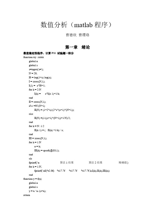
数值分析(matlab程序)曹德欣曹璎珞第一章绪论数值稳定性程序,计算P11 试验题一积分function try_stableglobal nglobal aa=input('a=');N = 20;I0 = log(1+a)-log(a);I = zeros(N,1);I(1) = -a*I0+1;for k = 2:NI(k) = - a*I(k-1)+1/k;endII = zeros(N,1);if a>=N/(N+1)II(N) = (1+2*a)/(2*a*(a+1)*(N+1));elseII(N) =(1/((a+1)*(N+1))+1/N)/2;endfor k = N:-1:2II(k-1) = ( - II(k) +1/k) / a;endIII = zeros(N,1);for k = 1:Nn = k;III(k) = quadl(@f,0,1);endclcfprintf('\n 算法1结果算法2结果精确值') for k = 1:N,fprintf('\nI(%2.0f) %17.7f %17.7f %17.7f',k,I(k),II(k),III(k)) endfunction y = f(x)global nglobal ay = x.^n./(a+x);return第二章非线性方程求解下面均以方程y=x^4+2*x^2-x-3为例:1、二分法function y=erfen(a,b,esp)format longif nargin<3 esp=1.0e-4;endif fun(a)*fun(b)<0n=1;c=(a+b)/2;while c>espif fun(a)*fun(c)<0b=c;c=(a+b)/2;elseif fun(c)*fun(b)<0a=c;c=(a+b)/2;else y=c; esp=10000;endn=n+1;endy=c;elseif fun(a)==0y=a;elseif fun(b)==0y=b;else disp('these,nay not be a root in the intercal')endnfunction y=fun(x)y=x^4+2*x^2-x-3;2、牛顿法function y=newton(x0)x1=x0-fun(x0)/dfun(x0);n=1;while (abs(x1-x0)>=1.0e-4) & (n<=100000000)x0=x1;x1=x0-fun(x0)/dfun(x0);n=n+1;endy=x1nfunction y=fun(x)y=x^4+2*x^2-x-3; 3、割线法function y=gexian(x0,x1)x2=x1-fun(x1)*(x1-x0)/(fun(x1)-fun(x0)); %根据初始XO 和X1求X2 n=1;while (abs(x1-x0)>=1.0e-4) & (n<=100000000) %判断两个条件截止 x0=x1; %将x1赋给x0 x1=x2; %将x2赋给x1 x2=x1-fun(x1)*(x1-x0)/(fun(x1)-fun(x0)); %迭代运算 n=n+1; end y=x2 nfunction y=fun(x)y=x^4+2*x^2-x-3;第四章题目:推导外推样条公式:⎪⎪⎪⎪⎪⎪⎪⎭⎫ ⎝⎛=⎪⎪⎪⎪⎪⎪⎭⎫ ⎝⎛⎪⎪⎪⎪⎪⎪⎭⎫ ⎝⎛--------1232123211223322~~~~~22~n n n n n n n n d d d d M M M Mδμλμλμλδ,并编写程序与Matlab 的Spline 函数结果进行对比,最后调用追赶法解方程组。
数值分析matlab程序
数值分析(matlab程序) 曹德欣 曹璎珞 第一章 绪论 数值稳定性程序,计算P11 试验题一积分 function try_stable global n global a a=input('a='); N = 20; I0 = log(1+a)-log(a); I = zeros(N,1); I(1) = -a*I0+1; for k = 2:N I(k) = - a*I(k-1)+1/k; end II = zeros(N,1); if a>=N/(N+1) II(N) = (1+2*a)/(2*a*(a+1)*(N+1)); else II(N) =(1/((a+1)*(N+1))+1/N)/2; end for k = N:-1:2 II(k-1) = ( - II(k) +1/k) / a; end III = zeros(N,1); for k = 1:N n = k; III(k) = quadl(@f,0,1); end clc fprintf('\n 算法1结果 算法2结果 精确值') for k = 1:N, fprintf('\nI(%2.0f) %17.7f %17.7f %17.7f',k,I(k),II(k),III(k)) end function y = f(x) global n global a y = x.^n./(a+x); return 第二章 非线性方程求解 下面均以方程y=x^4+2*x^2-x-3为例: 1、二分法 function y=erfen(a,b,esp) format long if nargin<3 esp=1.0e-4; end if fun(a)*fun(b)<0 n=1; c=(a+b)/2; while c>esp if fun(a)*fun(c)<0 b=c; c=(a+b)/2; elseif fun(c)*fun(b)<0 a=c; c=(a+b)/2; else y=c; esp=10000; end n=n+1; end y=c; elseif fun(a)==0 y=a; elseif fun(b)==0 y=b; else disp('these,nay not be a root in the intercal') end n function y=fun(x) y=x^4+2*x^2-x-3; 2、牛顿法 function y=newton(x0) x1=x0-fun(x0)/dfun(x0); n=1; while (abs(x1-x0)>=1.0e-4) & (n<=100000000) x0=x1; x1=x0-fun(x0)/dfun(x0); n=n+1; end y=x1 n function y=fun(x) y=x^4+2*x^2-x-3; 3、割线法 function y=gexian(x0,x1) x2=x1-fun(x1)*(x1-x0)/(fun(x1)-fun(x0)); %根据初始XO和X1求X2 n=1; while (abs(x1-x0)>=1.0e-4) & (n<=100000000) %判断两个条件截止 x0=x1; %将x1赋给x0 x1=x2; %将x2赋给x1 x2=x1-fun(x1)*(x1-x0)/(fun(x1)-fun(x0)); %迭代运算 n=n+1; end y=x2 n function y=fun(x) y=x^4+2*x^2-x-3;
同济大学数值分析matlab编程题汇编
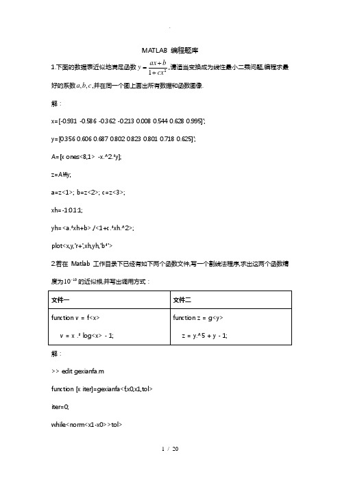
MATLAB 编程题库1.下面的数据表近似地满足函数21cxb ax y ++=,请适当变换成为线性最小二乘问题,编程求最好的系数c b a ,,,并在同一个图上画出所有数据和函数图像.解:x=[-0.931 -0.586 -0.362 -0.213 0.008 0.544 0.628 0.995]';y=[0.356 0.606 0.687 0.802 0.823 0.801 0.718 0.625]';A=[x ones<8,1> -x.^2.*y];z=A\y;a=z<1>; b=z<2>; c=z<3>;xh=-1:0.1:1;yh=<a.*xh+b>./<1+c.*xh.^2>;plot<x,y,'r+',xh,yh,'b*'>2.若在Matlab 工作目录下已经有如下两个函数文件,写一个割线法程序,求出这两个函数精度为1010-的近似根,并写出调用方式:解:>> edit gexianfa.mfunction [x iter]=gexianfa<f,x0,x1,tol>iter=0;while<norm<x1-x0>>tol>iter=iter+1;x=x1-feval<f,x1>.*<x1-x0>./<feval<f,x1>-feval<f,x0>>; x0=x1;x1=x;end>> edit f.mfunction v=f<x>v=x.*log<x>-1;>> edit g.mfunction z=g<y>z=y.^5+y-1;>> [x1 iter1]=gexianfa<'f',1,3,1e-10>x1 =1.7632iter1 =6>> [x2 iter2]=gexianfa<'g',0,1,1e-10>x2 =0.7549iter2 =83.使用GS迭代求解下述线性代数方程组:解:>> edit gsdiedai.mfunction [x iter]=gsdiedai<A,x0,b,tol>D=diag<diag<A>>;L=D-tril<A>;U=D-triu<A>;iter=0;x=x0;while<<norm<b-A*x>./norm<b>>>tol> iter=iter+1;x0=x;x=<D-L>\<U*x0+b>;end>> A=[5 2 1;-1 4 2;1 -3 10];>> b=[-12 10 3]';>>tol=1e-4;>>x0=[0 0 0]';>> [x iter]=gsdiedai<A,x0,b,tol>;>>xx =-3.09101.23720.9802>>iteriter =64.用四阶Range-kutta方法求解下述常微分方程初值问题〔取步长h=0.01 解:>> edit ksf2.mfunction v=ksf2<x,y>v=y+exp<x>+x.*y;>> a=1;b=2;h=0.01;>> n=<b-a>./h;>> x=[1:0.01:2];>>y<1>=2;>>fori=2:<n+1>k1=h*ksf2<x<i-1>,y<i-1>>;k2=h*ksf2<x<i-1>+0.5*h,y<i-1>+0.5*k1>;k3=h*ksf2<x<i-1>+0.5*h,y<i-1>+0.5*k2>;k4=h*ksf2<x<i-1>+h,y<i-1>+k3>;y<i>=y<i-1>+<k1+2*k2+2*k3+k4>./6;end>>y调用函数方法>> edit Rangekutta.mfunction [x y]=Rangekutta<f,a,b,h,y0>x=[a:h:b];n=<b-a>/h;y<1>=y0;fori=2:<n+1>k1=h*<feval<f,x<i-1>,y<i-1>>>;k2=h*<feval<f,x<i-1>+0.5*h,y<i-1>+0.5*k1>>;k3=h*<feval<f,x<i-1>+0.5*h,y<i-1>+0.5*k2>>;k4=h*<feval<f,x<i-1>+h,y<i-1>+k3>>;y<i>=y<i-1>+<k1+2*k2+2*k3+k4>./6;end>> [x y]=Rangekutta<'ksf2',1,2,0.01,2>;>>y5.取0.2h =,请编写Matlab 程序,分别用欧拉方法、改进欧拉方法在12x ≤≤上求解初值问题。
数值分析matlab实验报告

数值分析matlab实验报告《数值分析MATLAB实验报告》摘要:本实验报告基于MATLAB软件进行了数值分析实验,通过对不同数学问题的数值计算和分析,验证了数值分析方法的有效性和准确性。
实验结果表明,MATLAB在数值分析领域具有较高的应用价值和实用性。
一、引言数值分析是一门研究利用计算机进行数值计算和分析的学科,其应用范围涵盖了数学、物理、工程等多个领域。
MATLAB是一种常用的数值计算软件,具有强大的数值分析功能,能够进行高效、准确的数值计算和分析,因此在科学研究和工程实践中得到了广泛的应用。
二、实验目的本实验旨在通过MATLAB软件对数值分析方法进行实验验证,探究其在不同数学问题上的应用效果和准确性,为数值分析方法的实际应用提供参考和指导。
三、实验内容1. 利用MATLAB进行方程求解实验在该实验中,利用MATLAB对给定的方程进行求解,比较数值解和解析解的差异,验证数值解的准确性和可靠性。
2. 利用MATLAB进行数值积分实验通过MATLAB对给定函数进行数值积分,比较数值积分结果和解析积分结果,验证数值积分的精度和稳定性。
3. 利用MATLAB进行常微分方程数值解实验通过MATLAB对给定的常微分方程进行数值解,比较数值解和解析解的差异,验证数值解的准确性和可靠性。
四、实验结果与分析通过对以上实验内容的实际操作和分析,得出以下结论:1. 在方程求解实验中,MATLAB给出的数值解与解析解基本吻合,验证了MATLAB在方程求解方面的高准确性和可靠性。
2. 在数值积分实验中,MATLAB给出的数值积分结果与解析积分结果基本吻合,验证了MATLAB在数值积分方面的高精度和稳定性。
3. 在常微分方程数值解实验中,MATLAB给出的数值解与解析解基本吻合,验证了MATLAB在常微分方程数值解方面的高准确性和可靠性。
五、结论与展望本实验通过MATLAB软件对数值分析方法进行了实验验证,得出了数值分析方法在不同数学问题上的高准确性和可靠性。
数值分析与matlab——11_pdes

Chapter11Partial DifferentialEquationsA wide variety of partial differential equations occur in technical computing.We cannot begin to cover them all in this book.In this chapter we limit ourselves to three model problems for second order partial differential equations in one or two space dimensions.11.1Model ProblemsAll the problems we consider involve the Laplacian operator which,in one space dimension,is=∂2∂xand in two space dimensions is=∂2∂x2+∂2∂y2We let x denote the single variable x in one dimension and the pair of variables (x,y)in two dimensions.Thefirst model problem is the Poisson equation.This elliptic equation does not involve a time variable,and so describes the steady-state,quiescent behavior of a model variable.u=f( x)There are no initial conditions.The second model problem is the heat equation.This parabolic equation occurs in models involving diffusion and decay.∂u∂t= u−f( x)The initial condition isu( x,0)=u0( x)12Chapter11.Partial Differential Equations The third model problem is the wave equation.This hyperbolic equation de-scribes how a disturbance travels through matter.If the units are chosen so that the wave propagation speed is equal to one,the amplitude of a wave satisfies∂2u∂t= uTypical initial conditions specify the initial amplitude and take the initial velocity to be zero.u( x,0)=u0( x),∂u∂t( x,0)=0In one dimension,all the problems take place on afinite interval on the x axis.In more than one space dimension,geometry plays a vital role.In two dimensions,all the problems take place in a bounded regionΩin the(x,y)plane.In all cases,f( x) and u0( x)are given functions of x.All the problems involve boundary conditions where the value of u or some partial derivative of u is specified on the boundary of Ω.Unless otherwise specified,we will take the boundary values to be zero. 11.2Finite Difference MethodsBasicfinite difference methods for approximating solutions to these problems use a uniform mesh with spacing h.In one dimension,for the interval a≤x≤b,the spacing is h=(b−a)/(m+1),and the mesh points arex i=a+ih,i=0,...,m+1The second derivative with respect to x is approximated by the3-point centered second difference,h u(x)=u(x+h)−2u(x)+u(x−h)hIn two dimensions,the mesh is the set of points(x i,y j)=(ih,jh)that lie within the regionΩ.Approximating the partial derivatives with centered second differences gives the5-point discrete Laplacianh u(x,y)=u(x+h,y)−2u(x,y)+u(x−h,y)h+u(x,y+h)−2u(x,y)+u(x,y−h)hAlternate notation uses P=(x,y)for a mesh point and N=(x,y+h),E= (x+h,y),S=(x,y−h),and W=(x−h,y)for its four neighbors in the four compass directions.The discrete Laplacian ish u(P)=u(N)+u(W)+u(E)+u(S)−4u(P)h2Thefinite difference Poisson problem involvesfinding values of u so that h u( x)=f( x)11.2.Finite Difference Methods3 for each point x on the mesh.If the source term f( x)is zero,Poisson’s equation is called Laplace’s equation.h u(x)=0In one dimension,Laplace’s equation has only trivial solutions.The value of u at a mesh point x is the average of the values of u at its left and right neighbors,so u(x) must be a linear function of x.Taking the boundary conditions into consideration implies that u(x)is the linear function connecting the two boundary values.If the boundary values are zero,then u(x)is identically zero.In more than one dimension, solutions to Laplace’s equation are called harmonic functions and are not simply linear functions of x.Thefinite difference heat and wave equations also make use offirst and second differences in the t direction.Letδdenote the length of a time step.For the heat equation,we use a difference scheme that corresponds to Euler’s method for ordinary differential equationsu( x,t+δ)−u( x,t)= h u( x)δStarting with the initial conditions u( x,0)=u0( x),we can step from any value of t to t+δwithu( x,t+δ)=u( x,t)+δ h u( x,t)for all of the mesh points x in the region.The boundary conditions supply values on the boundary or outside the region.This method is explicit because each new value of u can be computed directly from values of u at the previous time step.More complicated methods are implicit because they involve the solution of systems of equations at each step.For the wave equation,we can use a centered second difference in t.u( x,t+δ)−2u( x,t)+u( x,t−δ)= h u( x,t)δ2This requires two“layers”of values of the solution,one at t−δand one at t.In our simple model problem,the initial condition∂u( x,0)=0∂tallows use to start with both u( x,0)=u0( x)and u( x,δ)=u0( x).We compute subsequent layers withu( x,t+δ)=2u( x,t)−u( x,t−δ)+δ2 h u( x,t)for all of the mesh points x in the region.The boundary conditions supply values on the boundary or outside the region.Like our scheme for the heat equation,this method for solving the wave equation is explicit.4Chapter11.Partial Differential Equations 11.3Matrix RepresentationIf a one-dimensional mesh function is represented as a vector,the one-dimensional difference operator h becomes the tridiagonal matrix,1 h2−211−211−21.........1−211−2This matrix is symmetric.(It is also negative definite.)Most importantly, even if there are thousands of interior mesh points,there are at most three nonzero elements in each row and column.Such matrices are the prime examples of sparse matrices.When computing with sparse matrices,it is important to use data struc-tures that store only the locations and values of the nonzero elements.With u represented as a vector and h2 h as a matrix A,the Poisson problem becomesAu=bwhere b is a vector(the same size as u)containing the values of h2f(x)at the interior mesh points.Thefirst and last components of b would also include any nonzero boundary values.In Matlab,the solution to the discrete Poisson problem is computed using sparse backslash,which takes advantage of the sparsity in A.u=A\bThe situation for meshes in two-dimensions is more complicated.Let’s number the interior mesh points inΩfrom top to bottom and from left to right.For example, the numbering of an L-shaped region would beL=000000000000159131721303948002610141822314049003711151923324150004812162024334251000000025344352000000026354453000000027364554000000028374655000000029384756000000000000The zeros are points on the boundary or outside the region.With this numbering, the values of any function defined on the interior of the region can be reshaped into a long column vector.In this example,the length of the vector is56.11.3.Matrix Representation5If a two-dimensional mesh function is represented as a vector,thefinite dif-ference Laplacian becomes a matrix.For example,at point number43, h2 h u(43)=u(34)+u(42)+u(44)+u(52)−4u(43)If A is the corresponding matrix,then its43rd row would havefive nonzero elements: a43,34=a43,42=a43,44=a43,52=1,and a43,43=−4A mesh point near the boundary has only two or three interior neighbors,so the corresponding row of A has only three or four nonzero entries.The complete matrix A has−4’s on its diagonal,four1’s offthe diagonal in most of its rows,two or three1’s offthe diagonal in some of its rows,and zeros elsewhere.For the example region above,A would be56-by-56.Here is A if there are only16interior points.A=-41100000000000001-40100000000000010-41100000000000011-40100000000000010-41100000000000011-40100000000000010-41000100000000011-41000100000000001-41000100000000001-41000100000000001-40000100000010000-41000000000010001-41000000000010001-41000000000010001-41000000000010001-4This matrix is symmetric,negative definite,and sparse.There are at most five nonzero elements in each row and column.Matlab has two functions that involve the discrete Laplacian,del2and delsq.If u is a two-dimensional array representing a function u(x,y),then del2(u) computes h u,scaled by h2/4,at interior points and uses one-sided formulae at points near the boundary.For example,the function u(x,y)=x2+y2has u=4. The statementsh=1/20;[x,y]=meshgrid(-1:h:1);u=x.^2+y.^2;d=(4/h^2)*del2(u);produce an array d,the same size as x and y,with all the elements equal to4.6Chapter11.Partial Differential Equations If G is a two-dimensional array specifying the numbering of a mesh,then A= -delsq(G)is the matrix representation of the operator h2 h on that mesh.The mesh numbering for several specific regions is generated by numgrid.For example, m=5L=numgrid(’L’,2*m+1)generates the L-shaped mesh with56interior points shown above.And, m=3A=-delsq(numgrid(’L’,2*m+1))generates the16-by-16matrix A shown above.The function inregion can also generate mesh numberings.For example,the coordinates of the vertices of the L-shaped domain arexv=[0011-1-10];yv=[0-1-11100];The statement[x,y]=meshgrid(-1:h:1);generates a square grid of width h.The statement[in,on]=inregion(x,y,xv,yv);generates arrays of zeros and ones that mark the points that are contained in the domain,including the boundary,as well as those that are strictly on the boundary. The statementsp=find(in-on);n=length(p);L=zeros(size(x));L(p)=1:n;number the n interior points from top to bottom and left to right.The statement A=-delsq(L);generates the n-by-n sparse matrix representation of the discrete Laplacian on the mesh.With u represented as a vector with n components,the Poisson problem be-comesAu=bwhere b is a vector(the same size as u)containing the values of h2f(x,y)at the interior mesh points.The components of b that correspond to mesh points with neighbors on the boundary or outside the region also include any nonzero boundary values.As in one dimension,the solution to the discrete Poisson problem is computed using sparse backslashu=A\b11.4.Numerical Stability7 11.4Numerical StabilityThe time-dependent heat and wave equations generate a sequence of vectors,u(k), where the k denotes the k th time step.For the heat equation,the recurrence is u(k+1)=u(k)+σAu(k)whereσ=δh2This can be writtenu(k+1)=Mu(k)whereM=I+σAIn one dimension,the iteration matrix M has1−2σon the diagonal and one or twoσ’s offthe diagonal in each row.In two dimensions M has1−4σon the diagonal and two,three,or fourσ’s offthe diagonal in each row.Most of the row sums in M are equal to1;a few are less than1.Each element of u(k+1)is a linear combination of elements of u(k)with coefficients that add up to1or less.Now,here is the key observation.If the elements of M are nonnegative,then the recurrence is stable.In fact,it is dissipative.Any errors or noise in u(k)are not magnified in u(k+1).But if the diagonal elements of M are negative,then the recurrence can be unstable.Error and noise,including roundofferror and noise in the initial conditions,can be magnified with each time step.Requiring1−2σor1−4σto be positive leads to a very important stability condition for this explicit method for the heat equation.In one dimensionσ≤1 2And,in two dimensionsσ≤1 4If this condition is satisfied,the iteration matrix has positive diagonal elements and the method is stable.Analysis of the wave equation is a little more complicated because it involves three levels,u(k+1),u(k),and u(k−1).The recurrence isu(k+1)=2u(k)−u(k−1)+σAu(k)whereσ=δ2 h2The diagonal elements of the iteration matrix are now2−2σ,or2−4σ.In one dimension,the stability condition isσ≤18Chapter11.Partial Differential Equations And,in two dimensionsσ≤1 2These stability conditions are known as the CFL conditions,after Courant, Friedrichs and Lewy,who wrote a now paper in1928that usedfinite difference methods to prove existence of solutions to the PDEs of mathematical physics.Sta-bility conditions are restrictions on the size of the time step,δ.Any attempt to speed up the computation by taking larger time steps is likely to be disastrous.For the heat equation,the stability condition is particularly severe—the time step must be smaller than the square of the space mesh width.More sophisticated methods, often involving some implicit equation solving at each step,have less restrictive or unlimited stability conditions.The M-file pdegui illustrates the concepts discussed in this chapter by offering the choice among several domains and among the model PDEs.For Poisson’s equation,pdegui uses sparse backslash to solveh u=1in the chosen domain.For the heat and wave equations,the stability parameter σcan be varied.If the critical value,0.25for the heat equation and0.50for the wave equation,is exceeded by even a small amount,the instability rapidly becomes apparent.You willfind much more powerful capabilities in the Matlab Partial Differ-ential Equation Toolbox.11.5The L-shaped MembraneSeparating out periodic time behavior in the wave equation leads to solutions of theformu( x,t)=cos(√λt)v( x)The functions v( x)depend uponλ.They satisfyv+λv=0and are zero on the boundary.The quantitiesλthat lead to nonzero solutions are the eigenvalues and the corresponding functions v( x)are the eigenfunctions or modes.They are determined by the physical properties and the geometry of each particular situation.The square roots of the eigenvalues are resonant frequencies.A periodic external driving force at one of these frequencies generates an unboundedly strong response in the medium.Any solution of wave equation can be expressed as a linear combination of these eigenfunctions.The coefficients in the linear combination are obtained from the initial conditions.In one dimension,the eigenvalues and eigenfunctions are easily determined. The simplest example is a violin string,heldfixed at the ends of the interval of lengthπ.The eigenfunctions arev k(x)=sin(kx)11.5.The L-shaped Membrane9 The eigenvalues are determined by the boundary condition,v k(π)=0.Hence,k must be an integer andλk=k2.If the initial condition,u0(x),is expanded in a Fourier sine series,u0(x)=ka k sin(kx)then the solution to the wave equation isu(x,t)=ka k cos(kt)sin(kx)=k a k cos(λk t)v k(x)In two dimensions,an L-shaped region formed from three unit squares is in-teresting for several reasons.It is one of the simplest geometries for which solutions to the wave equation cannot be expressed analytically,so numerical computation is necessary.Furthermore,the270◦nonconvex corner causes a singularity in the solution.Mathematically,the gradient of thefirst eigenfunction is unbounded near the corner.Physically,a membrane stretched over such a region would rip at the corner.This singularity limits the accuracy offinite difference methods with uni-form grids.The MathWorks has adopted a surface plot of thefirst eigenfunction of the L-shaped region as the company logo.The computation of this eigenfunction involves several of the numerical techniques we have described in this book.Simple model problems involving waves on an L-shaped region include an L-shaped membrane,or L-shaped tambourine,and a beach towel blowing in the wind,constrained by a picnic basket on one fourth of the towel.A more practical example involves ridged microwave waveguides.One such device,shown infigure 11.1,is a waveguide-to-coax adapter.The active region is the channel with the H-shaped cross section visible at the end of the adapter.The ridges increase the bandwidth of the guide at the expense of higher attenuation and lower power-handling capability.Symmetry of the H about the dotted lines shown in the contour plot of the electricfield implies that only one quarter of the domain needs to be considered and that the resulting geometry is our L-shaped region.The boundary conditions are different than our membrane problem,but the differential equation and the solution techniques are the same.Eigenvalues and eigenfunctions of the L-shaped domain can be computed by finite difference methods.The Matlab statementsm=200h=1/mA=delsq(numgrid(’L’,2*m+1))/h^2set up thefive-pointfinite difference approximation to the Laplacian on an200-by-200mesh in each of the three squares that make up the domain.The resulting sparse matrix A has order119201and594409nonzero entries.The statement10Chapter11.Partial Differential EquationsFigure11.1.A double-ridge microwave-to-coax adapter and its H-shaped region.Photo courtesy Advanced Technical Materials,Inc.[1].lambda=eigs(A,6,0)uses Arnoldi’s method from the Matlab implementation of ARPACK to compute thefirst six eigenvalues.It takes less than two minutes on a1.4GHz Pentium laptop to producelambda=9.6414715.1969419.7388029.5203331.9158341.47510The exact values are9.6397215.1972519.7392129.5214831.9126441.47451You can see that even with thisfine mesh and large matrix calculation,the computed eigenvalues are accurate to only three or four significant digits.If you try to get more accuracy by using afiner mesh and hence a larger matrix,the computation requires so much memory that the total execution time is excessive.For the L-shaped domain and similar problems,a technique using analytic solutions to the underlying differential equation is much more efficient and accu-11.5.The L-shaped Membrane 11rate than finite difference methods.The technique involves polar coordinates and fractional order Bessel functions.With parameters αand λ,the functions v (r,θ)=J α(√r )sin (αθ)are exact solutions to the polar coordinate version of eigenfunction equation,∂2v ∂r 2+1r ∂v ∂r +1r 2∂2v ∂θ2+λv =0For any value of λ,the functions v (r,θ)satisfy the boundary conditionsv (r,0)=0,and v (r,π/α)=0on the two straight edges of a circular sector with angle π/α.If √λis chosen to be a zero of the Bessel function,J α(√λ)=0,then v (r,θ)is also zero on the circle,r =1.Figure 11.2shows a few of the eigenfunctions of the circular sector with angle 3π/2.The eigenfunctions have been chosen to illustrate symmetry about 3π/4and π/2.8.949433.492714.355944.071120.714655.6455Figure 11.2.Eigenfunctions of the three-quarter disc.We approximate the eigenfunctions of the L-shaped domain and other regions with corners by linear combinations of the circular sector solutions,v (r,θ)= jc j J αj (√λr )sin (αj θ)The angle of the reentrant 270◦corner in the L-shaped region is 3π/2,or π/(2/3),so the values of αare integer multiples of 2/3,αj =2j3These functions v (r,θ)are exact solutions to the eigenfunction differential equation.There is no finite difference mesh involved.The functions also satisfy the boundary12Chapter11.Partial Differential Equations conditions on the two edges that meet at the reentrant corner.All that remains is to pick the parameterλand the coefficients c j so that the boundary conditions on the remaining edges are satisfied.A least squares approach involving the matrix singular value decomposition is used to determineλand the c j.Pick m points,(r i,θi),on the remaining edges of the boundary.Let n be the number of fundamental solutions to be used.Generate an m-by-n matrix A with elements that depend uponλ,A i,j(λ)=Jαj (√λr i)sin(αjθi),i=1,...,m,j=1,...,nThen,for any vector c,the vector Ac is the vector of boundary values,v(r i,θi). We want to make||Ac||small without taking||c||small.The SVD provides the solution.Letσn(A(λ))denote the smallest singular value of the matrix A(λ).and let λk denote a value ofλthat produces a local minima of the smallest singular value,λk=k-th minimizer(σn(A(λ)))Eachλk approximates an eigenvalue of the region.The corresponding right singular vector provides the coefficients for the linear combination,c=V(:,n).9.639715.197319.739231.912644.948549.3480Figure11.3.Eigenfunctions of the L-shaped region.It is worthwhile to take advantage of symmetries.It turns out that the eigen-functions fall into three symmetry classes,•Symmetric about the center line atθ=3π/4,so v(r,θ)=v(r,3π/2−θ).•Antisymmetric about the center line atθ=3π/4,so v(r,θ)=−v(r,3π/2−θ).•Eigenfunction of the square,so v(r,π/2)=0and v(r,π)=0.These symmetries allow us to restrict the values ofαj used in each expansion,Exercises13•αj =2j 3,j odd and not a multiple of 3.•αj =2j 3,j even and not a multiple of 3.•αj =2j3,j a multiple of 3.The M-file membranetx in the NCM directory computes eigenvalues and eigenfunc-tions of the L-membrane using these symmetries and a search for local minima of σn (A (λ)).The M-file membrane ,distributed with Matlab in the demos directory,uses an older version of the algorithm based on the QR decomposition instead of the SVD.Figure 11.3shows six eigenfunctions of the L-shaped region,with two from each of the three symmetry classes.They can be compared with the eigenfunctions of the sector shown in figure 11.2.By taking the radius of the sector to be 2/√π,both regions have the same area and the eigenvalues are comparable.The demo M-file logo makes a surf plot of the first eigenfunction,then adds lighting and shading to create the MathWorks logo.After being so careful to satisfy the boundary conditions,the logo uses only the first two terms in the circular sector expansion.This artistic license gives the edge of the logo a more interesting,curved shape.Exercises11.1.Let n be an integer and generate n -by-n matrices A ,D ,and I with thestatementse=ones(n,1);I=spdiags(e,0,n,n);D=spdiags([-e e],[01],n,n);A =spdiags([e -2*e e],[-101],n,n);(a)For an appropriate value of h ,the matrix (1/h 2)A approximates h .Is the value of h equal to 1/(n −1),1/n ,or 1/(n +1)?(b)What does (1/h )D approximate?(c)What are D T D and DD T ?(d)What is A 2?(e)What is kron(A,I)+kron(I,A)?(f)Describe the output produced by plot(inv(full(-A)))?11.2.(a)Use finite differences to compute a numerical approximation to the solu-tion u (x )to the one-dimensional Poisson problemd 2u dx2=exp (−x 2)on the interval −1≤x ≤1.The boundary conditions are u (−1)=0and u (1)=0.Plot your solution.(b)If you have access to dsolve in the Symbolic Toolbox,or if you are very good at calculus,find the analytic solution of the same problem and compare it with your numerical approximation.14Chapter11.Partial Differential Equations 11.3.Reproduce the contour plot infigure11.1of thefirst eigenfunction of theH-shaped ridge waveguide formed from four L-shaped regions.11.4.Let h(x)be the function defined by the M-file humps(x).Solve four differentproblems involving h(x)on the interval0≤x≤1.Figure11.4.h(x)and u(x)(a)One-dimensional Poisson problem with humps as the source term.d2udx2=−h(x)Boundary conditionsu(0)=0,u(1)=0Make plots,similar tofigure11.4,of h(x)and u(x).Compare diff(u,2) with humps(x).(b)One-dimensional heat equation with humps as the source term.∂u ∂t =∂2u∂x+h(x)Initial valueu(0,x)=0Boundary conditionsu(0,t)=0,u(1,t)=0Create an animated plot of the solution as a function of time.What is the limit as t→∞of u(x,t)?(c)One-dimensional heat equation with humps as the initial value.∂u ∂t =∂2u∂x2Initial valueu(x,0)=h(x)Exercises15 Boundary conditionsu(0,t)=h(0),u(1,t)=h(1)Create an animated plot of the solution as a function of time.What is the limit as t→∞of u(x,t)?(d)One-dimensional wave equation with humps as the initial value.∂2u ∂t =∂2u∂xInitial valuesu(x,0)=h(x),∂u∂t(x,0)=0Boundary conditionsu(0,t)=h(0),u(1,t)=h(1)Create an animated plot of the solution as a function of time.For what values of t does u(x,t)return to its initial value h(x)?11.5.Let p(x,y)be the function defined by the M-file peaks(x,y).Solve fourdifferent problems involving p(x,y)on the square−3≤x≤3,−3≤y≤3.Figure11.5.p(x,y)and u(x,y)(a)Two-dimensional Poisson problem with peaks as the source term.∂2u ∂x2+∂2u∂y2=p(x,y)Boundary conditionsu(x,y)=0,if|x|=3,or|y|=3Make contour plots,figure similar tofigure11.5,of p(x,y)and u(x,y).16Chapter11.Partial Differential Equations(b)Two-dimensional heat equation with peaks as the source term.∂u ∂t =∂2u∂x2+∂2u∂y2−p(x,y)Initial valueu(x,y,0)=0Boundary conditionsu(x,y,t)=0,if|x|=3,or|y|=3Create an animated contour plot of the solution as a function of time.What is the limit as t→∞of u(x,t)?(c)Two-dimensional heat equation with peaks as the initial value.∂u ∂t =∂2u∂x2Initial valueu(x,y,0)=p(x,y)Boundary conditionsu(x,y,t)=p(x,y),if|x|=3,or|y|=3Create an animated contour plot of the solution as a function of time.What is the limit as t→∞of u(x,t)?(d)Two-dimensional wave equation with peaks as the initial value.∂2u ∂t2=∂2u∂x2Initial valuesu(x,y,0)=p(x,y),∂u∂t(x,y,0)=0Boundary conditionsu(x,y,t)=p(x,y),if|x|=3,or|y|=3Create an animated contour plot of the solution as a function of time.Does the limit as t→∞of u(x,t)exist?11.6.The method of lines is a convenient technique for solving time-dependentpartial differential equations.Replace all the spatial derivatives byfinite differences,but leave the time derivatives intact.Then use a stiffordinary differential equation solver on the resulting system.In effect,this is an im-plicit time-steppingfinite difference algorithm with the time step determinedExercises17 automatically and adaptively by the ODE solver.For our model heat and wave equations,the ODE systems are simply˙u=(1/h2)A uand¨u=(1/h2)A uThe matrix(1/h2)A represents h and u is the vector-valued function of t formed from all the elements u(x i,t)or u(x i,y j,t)at the mesh points.(a)The Matlab function pdepe implements the method of lines in a generalsetting.Investigate its use for our one-and two-dimensional model heat equations.(b)If you have access to the Partial Differential Equation Toolbox,investigateits use for our two-dimensional model heat and wave equations.(c)Implement your own method of lines solutions for our model equations.11.7.Answer the following questions about pdegui.(a)How does the number of points n in the grid depend upon the grid sizeh for the various regions?(b)How does the time step for the heat equation and for the wave equationdepend upon the grid size h?(c)Why are the contour plots of the solution to the Poisson problem and theeigenvalue problem with index=1similar?(d)How do the contour plots produced by pdegui of the eigenfunctions ofthe L-shaped domain compare with those produced bycontourf(membranetx(index))(e)Why are regions Drum1and Drum2interesting?Search the Web for“isospectral”and“Can you hear the shape of a drum?”.You shouldfind many articles and papers,including ones by Gordon,Webb and Wolpert[3], and by Driscoll[2].11.8.Add the outline of your hand that you obtained in exercise3.4as anotherregion to pdegui.Figure11.6shows one of the eigenfunctions of my hand.11.9.The electrostatic capacity of a regionΩis the quantityu(x,y)dxdyΩwhere u(x,y)is the solution to the Poisson problemu=−1inΩand u(x,y)=0on the boundary ofΩ(a)What is the capacity of the unit square?(b)What is the capacity of the L-shaped domain?(c)What is the capacity of your hand?11.10.The statements18Chapter11.Partial Differential EquationsFigure11.6.An eigenfunction of a hand.load pennyP=flipud(P)contour(P,1:12:255)colormap(copper)axis squareaccess afile in the Matlab demos directory and producefigure11.7.The data was obtained in1984at what was then the National Bureau of Standards by an instrument that makes precise measurements of the depth of a mold used to mint the U.S.one cent coin.Figure11.7.The depth of a mold used to mint the U.S.one cent coin.The NCM function pennymelt uses this penny data as the initial condition, u(x,y,0),for the heat equation and produces an animated,lighted surface plot of the solution,u(x,y,t).。
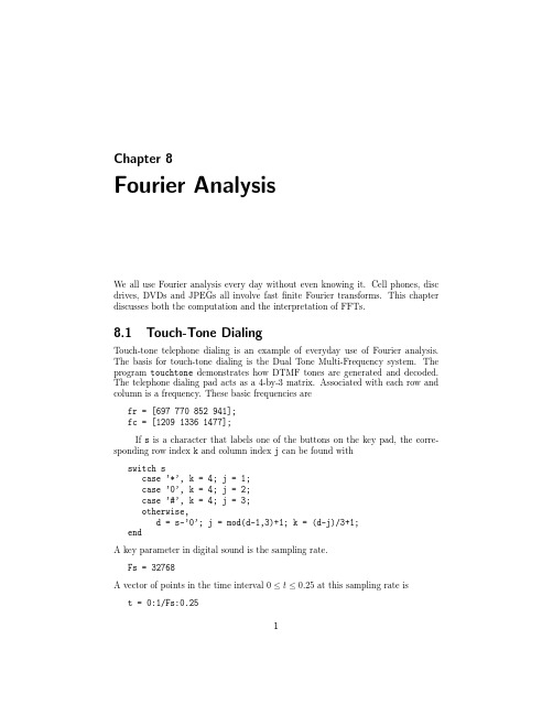
数值分析与matlab——08_fourier
4
600 400 200 0
Chapter 8. Fourier Analysis
600
800
1000
1200
1400
1600
Figure 8.3. FFT of the recorded signal p = abs(fft(y)); f = (0:n-1)*(Fs/n); plot(f,p); axis([500 1700 0 600]) The x-axis corresponds to frequency. The axis settings limit the display to the range of the DTMF frequencies. There are seven peaks, corresponding to the seven basic frequencies. This overall FFT shows that all seven frequencies are present someplace in the signal, but it does not help determine the individual digits. The touchtone program also lets you break the signal into eleven equal segments and analyze each segment separately. Figure 8.4 is the display of the first segment.
1
0ห้องสมุดไป่ตู้
−1
1
2
3
4
5
6
7
8
9
Figure 8.2. Recording of an 11-digit telephone number This signal is noisy. You can even see small spikes on the graph at the times the buttons were clicked. It is easy to see that eleven digits were dialed, but on this scale, it is impossible to determine the specific digits. Figure 8.3 shows the magnitude of the FFT, the finite Fourier transform, of the signal, which is the key to determining the individual digits. The plot was produced with
(完整版)MATLAB数值分析实例
2016-2017 第一学期数值分析上机实验报告姓名: xxx学号: 20162…….学院:土木工程学院导师:………..联系电话:…………..指导老师:………..目录第一题 (1)1.1题目要求 (1)1.2程序编写 (1)1.3计算结果及分析 (2)第二题 (4)2.1题目要求 (4)2.2程序编写 (4)2.3计算结果及分析 (6)第三题 (7)3.1题目要求 (7)3.2程序编写 (7)3.3计算结果及分析 (8)第四题 (9)4.1题目要求 (9)4.2程序编写 (9)4.3计算结果及分析 (10)第五题 (11)5.1题目要求 (11)5.2程序编写 (12)5.3计算结果及分析 (13)第六题 (17)6.1题目要求 (17)6.2程序编写 (17)6.3计算结果及分析 (18)6.4程序改进 (18)第一题选做的是第(1)小问。
1.1题目要求编出不动点迭代法求根的程序;把??3+4??2-10=0写成至少四种??=g(??)的形式,取初值??0=1.5,进行不动点迭代求根,并比较收敛性及收敛速度。
1.2程序编写1.3计算结果及分析①第一种迭代公式:??=??3+4??2+??-10;matlab计算结果如下:(以下为命令行窗口的内容)2;matlab计算结果如下:②第二种迭代公式:??=√(10-??3)/4(以下为命令窗口内容)2;matlab计算结果如下:③第三种迭代公式:??=√10(??+4)?(以下为命令窗口内容)④第四种迭代公式:??=10(??2+4??)?;matlab计算结果如下:(以下为命令窗口内容)上述4种迭代公式,1、4两种由于在x真实值附近|g`(x)|>1,不满足迭代局部收敛条件,所以迭代序列不收敛。
对于2、3两种式子,由于在x真实值附近|g`(x)|<=L<1,满足迭代局部收敛条件,所以迭代序列收敛。
对于2、3两迭代公式,由于L3<L2,所以第3个迭代公式比第2个迭代公式收敛更快。
数值分析Matlab作业

数值分析编程作业2012年12月第二章14.考虑梯形电阻电路的设计,电路如下:电路中的各个电流{i1,i2,…,i8}须满足下列线性方程组:121232343454565676787822/252025202520252025202520250i i V R i i i i i i i i i i i i i i i i i i i i -=-+-=-+-=-+-=-+-=-+-=-+-=-+=这是一个三对角方程组。
设V=220V ,R=27Ω,运用追赶法,求各段电路的电流量。
Matlab 程序如下:function chase () %追赶法求梯形电路中各段的电流量 a=input('请输入下主对角线向量a='); b=input('请输入主对角线向量b='); c=input('请输入上主对角线向量c='); d=input('请输入右端向量d='); n=input('请输入系数矩阵维数n='); u(1)=b(1); for i=2:nl(i)=a(i)/u(i-1); u(i)=b(i)-c(i-1)*l(i); endy(1)=d(1); for i=2:ny(i)=d(i)-l(i)*y(i-1); endx(n)=y(n)/u(n); i=n-1; while i>0x(i)=(y(i)-c(i)*x(i+1))/u(i); i=i-1; end x输入如下:请输入下主对角线向量a=[0,-2,-2,-2,-2,-2,-2,-2]; 请输入主对角线向量b=[2,5,5,5,5,5,5,5];请输入上主对角线向量c=[-2,-2,-2,-2,-2,-2,-2,0]; 请输入方程组右端向量d=[220/27,0,0,0,0,0,0,0]; 请输入系数矩阵阶数n=8 运行结果如下:x = 8.1478 4.0737 2.0365 1.0175 0.5073 0.2506 0.1194 0.0477第三章14.试分别用(1)Jacobi 迭代法;(2)Gauss-Seidel 迭代法解线性方程组1234510123412191232721735143231211743511512x x x x x ⎡⎤⎡⎤⎡⎤⎢⎥⎢⎥⎢⎥---⎢⎥⎢⎥⎢⎥⎢⎥⎢⎥⎢⎥=--⎢⎥⎢⎥⎢⎥--⎢⎥⎢⎥⎢⎥⎢⎥⎢⎥⎢⎥---⎣⎦⎣⎦⎣⎦ 迭代初始向量(0)(0,0,0,0,0)T x =。
Matlab第2次作业_数值

1 •设a=(1,2,3),b=(2,4,3), 分别计算 a./b , a.\b , a/b , a\b ,分析结果的意义。
解:>> a=[1,2,3];>> b=[2,4,3];>> a./b 【意义】矩阵内的元素-- 对应的作 -运算bans =0.5000 0.5000 1.0000>> a.\b 【意义】矩阵内的元素-- 对应的作 -运算bans =2 2 1>> a/b 【意义】矩阵整体xb=a,求x;ans =0.6552>> a\b 【意义】矩阵整体ax=b,求x;ans =0 0 00 0 00.6667 1.3333 1.00002 •用矩阵除法解下列线性方程组,并判断解的意义4 1 1 % 91 32 6 X2 2 ;11 5 3 x3解:>> a=[4 1 -1;3 2 -6;1 -5 3];>> b=[9;-2;1];>> a\bans =2.38301.48942.0213【意义】最小二乘法求解ax=b的近似解X iX2解:>> a=[4 1;3 2;1 -5];>> b=[1;1;1];>> a\b ans =0.3311-0.1219【意义】最小二乘法求解ax=b的近似解2 1 1 1%X2 13 1 2 1 1x3 21 12 1 3x4解:>> a=[2 1 -1 1;1 2 1 -1;1 1 2 1>> b=[1;2;3];>> a\bans =11【意义】最小二乘法求解欠定方程ax=b的解3.(人口流动趋势)对城乡人口流动作年度调查,发现有一个稳定的朝向城镇流动的趋势,每年农村居民的5赠居城镇而城镇居民的1%i出,现在总人口的20%u于城镇。
加入城乡总人口保持不变,并且人口流动的这种趋势继续下去,那么(1)一年以后住在城镇人口所占比例是什么?两年以后呢?十年以后呢?(2)很多年以后呢?(3)如果现在总人口70%u于城镇,很多年以后城镇人口所占比例是什么?(4)计算转移矩阵的最大特征值级对应的特征向量,与问题(2),(3)有何关系?解: (1)>>a=[0.99 0.05;0.01 0.95]; x0=[0.2 0.8] ';>> x1=a*x0,x2=a A2*x0,x10=a A10*x0x1 =0.23800.7620 x2 =0.27370.7263 x10 =0.49220.5078(2)【方法一:循环的方法】>> x=x0;for i=1:1000,x=a*x;en d,xx =0.83330.1667【方法二:累乘的方法】>> x=a A1000*x0x =0.83330.1667【注】若求ax=x,即(a-I ) x=0的非零解,得结果如下>> cleara=[0. 99 0. 05:0.01 0. 95] : b=*y^(2, 2):-0*0606-0.1M1错误原因在于,非零解是一组基础解系,不能具体确定x的值。
matlab与数值分析

matlab与数值分析实验指导书:Matlab 软件与数值计算Matlab 的含义是矩阵实验室(Matrix Laboratory),是由美国MathWork公司于1984年推出的一套高性能的数值计算软件,由于它具有使用方便,用户界面友好的特征,能集数值分析,矩阵计算,信号处理和图形显示于一身,更有多种用户工具包可选用,深受计算工作者和工程技术人员的亲睐,目前使用十分广泛.本书特选用Matlab作为数值分析的演示及实验的软件环境.本章只介绍与本书演示及实验有关的Matlab知识,更详细的Matlab知识可参考相关书籍.§10.1 矩阵与数组1.行向量>> x=[2 -3 1] %中间用空格将数据分开,也可用逗号分开x =2 -3 1 %显示输出结果2.列向量>> y=[3 -1 5]' % ' 表示转置y =3-153.矩阵输入>>A=[1 3 2;5 4 6;7 9 8] % ;表示换行A =1 3 25 4 67 9 84.矩阵转置B =1 5 73 4 92 6 85. 单位阵>> I=eye(3) % 3 表示矩阵是3阶方阵I =1 0 00 1 00 0 16. 零矩阵>> Z=zeros(3)0 0 00 0 00 0 07. 矩阵加减法>> C=A+B,C =2 8 98 8 159 15 16>>D=A-BD =0 -2 -52 0 -35 3 08. 矩阵乘法>> E=A*B,E =29 77 11950 119 1949. 数组输入除上述的矩阵输入法外,数组还可以有如下输入法:(1) 等差输入数组=初值:增量:终值>>a=1:2:10a =1 3 5 7 9增量为1时,可以省略>> a=1:5a =1 2 3 4 5(2) 等分输入法数组=linspace(初值,终值,等分点数)>> a=linspace(0,10,5)a =0 2.5000 5.0000 7.5000 10.000010. 点运算数组的点乘运算是对应分量相乘;矩阵的点乘是对应元素相乘,类似的运算还有点除(./)和点乘方(.^).如:>> x=1:5x =1 2 3 4 5>> y=-2:2-2 -1 0 1 2>>z=x.*yz =-2 -2 0 4 10§10.2 函数运算和作图10.2.1基本初等函数1.三角函数: sin(x), cos(x), tan(x);2.反三角函数: asin(x), acos(x), atan(x);3.指数函数e x: exp(x) ;4.对数函数:(1)自然对数ln x:log(x);(2)常用对数lg x: log10(x);log()x: log2(x);(3)以2为底的对数25.开平方函数: sqrt(x);6.绝对值函数:abs(x)7.计算一般函数值: eval(f )其中f是一个函数表达式的字符串>> f='x.*sin(x)';>> x=1:10;>>y= eval(f)y =Columns 1 through 90.8415 1.8186 0.4234 -3.0272 -4.7946 -1.6765 4.5989 7.9149 3.7091 Column 10-5.440210.2.2 多项式函数1.多项式的表示多项式可用一个向量表示,其分量为其降幂排列的系数.如32x x-+可表为p=[1 –3 0 5]352.多项式求值polyval(p,x)>> p=[1 –3 0 5];>> x=1:10;>> y=polyval(p,x)y =3 1 5 21 55 113 201 325 491 705 3. 多项式的零点roots(p)>> roots(p)ans =2.0519 + 0.5652i2.0519 - 0.5652i-1.10384.方阵A的特征多项式poly(A) >> A=[3 1 2;1 3 2;1 2 3]>> p=poly(A)p =1.0000 -9.0000 20.0000 -12.0000>> roots(ans)ans =6.00002.00001.000010.2.3 矩阵函数1. 矩阵的行列式>>A=[1 3 2;5 4 6;7 9 8]A =1 3 25 4 67 9 8>>d=det(A),d =2. 矩阵的逆>> B=inv(A),B =-1.2222 -0.3333 0.55560.1111 -0.3333 0.22220.9444 0.6667 -0.61113. LU分解命令格式: [L U P]=lu(A)说明:这里L是单位下三角矩阵,U是上三角矩阵,P是置换阵,这是因为本命令中默认加上了按列选主元素.如命令中省略P, 则L不一定是单位下三角矩阵,而PL才是单位下三角矩阵. 例:>> [L U P]=lu(A)L =1.0000 0 00.7143 1.0000 00.1429 -0.7059 1.0000U =7.0000 9.0000 8.00000 -2.4286 0.28570 0 1.0588P =0 0 10 1 01 0 0>> [L U ]=lu(A)L =0.1429 -0.7059 1.00000.7143 1.0000 01.0000 0 07.0000 9.0000 8.00000 -2.4286 0.28570 0 1.05884. 矩阵范数命令格式: n1=norm(A,1), n2=norm(A,2), ninf=norm(A,inf)说明:这三个命令分别求A的1-范数,2-范数和-范数,其中n2=norm(A,2)也可写为n2=norm(A)例:>> A=[3 1 2;1 3 2;2 2 3];>> n1=norm(A,1)n1 =7>> n2=norm(A,2)n2 =6.3723>> ninf=norm(A,inf)ninf =75. 特征值分解命令格式: [Q,D]=eig(A),D=eig(A)说明:此命令可以求出方阵A的特征值和相应的特征向量.例:>> A=[3 1 2;1 3 2;2 2 3]A =3 1 21 3 22 2 3>> D=eig(A)D =0.62772.00006.3723>> [Q,D]=eig(A)Q =0.4544 0.7071 0.5418 0.4544 -0.7071 0.5418 -0.7662 0 0.6426D =0.6277 0 0 0 2.0000 0 0 0 6.372310.2.4 绘图命令1. 二维绘图函数plot ,常用和最简单的绘图工具(1) 格式: plot(x,y,’-r ’)(2) 说明:将x 和y 对应分量定义的点依次用红色实线联结(x,y 的维数必须一致). (3) 其中线型点型和色号可按下两表选择:表10.1线型符号点型符号实线-(减号) 实心圆点.虚线――(双减号)加号+点线:星号 *虚线间点-.(减号加点)空心圆点o (小写字母o )叉号 x (小写字母x )表10.2兰色红色黄色绿色 bryg(4) 绘图辅助命令利用以下命令可以为图形加上不同效果,注意以下命令必须放在相应的plot 命令之后.表10.3 title(‘…’) 在图形上方加标题xlabel(‘…’) 为X轴加说明ylabel(‘…’) 为Y轴加说明 grid 在图上显示虚线格标度text(x,y,‘…’) 在图中x,y 坐标处显示‘…’中的内容gtext( ‘…’) 在图中用光标确定位置处显示‘…’中的内容axis([xl,xu,yl,yu]) 用[]中四个实数定义x,y 方向显示范围 hold on 后面的plot 图形将叠加在一起hold off解除hold on 命令,后面plot 产生的图形将冲去原有图形例10.1 作出[-π,π]间函数2sin y x x =的图形x=-pi:0.05:pi; y=x.*x.*sin(2*x); plot(x,y,'-') grid2. 一元函数绘制函数命令fplot ,可绘制已定义函数在指定区间上的图象,与plot 命令类似,但能自适应地选择取值点.plot 的线型和色号选项依然适用.格式: fplot(f,[a,b]),其中f 是一个函数表达式的字符串,a,b 是x 取值的下界和上界.例10.2 作出[-π,π]间函数2sin y x x =的图形f='x.*x.*sin(2*x)' fplot(f,[-pi,pi])也可以作出与例10.1一样的图形.图10-13. 多窗口绘图函数subplot 格式:subplot(p,q,r)说明:将图形窗口分为p 行q 列共p ?q 个格子,在第r 个格子上画图,格子是从上到下,从左到右依次计数的.例10.3 作出[-1,1]间前四个Legendre 多项式的图形Legendre 多项式是定义在[-1,1]上的正交多项式系列,它可由下列递推公式生成:011112111(),(),()()().k k k p x p x x k kp x xp x p x k k +-==+=-++ x=-1:0.05:1p0=1+0*x;p1=x; p2=(3*x.^2-1)/2; p3=(5*x.^3-3*x)/2subplot(2,2,1);plot(x,p0) subplot(2,2,2);plot(x,p1) subplot(2,2,3);plot(x,p2) subplot(2,2,4);plot(x,p3)图10-210.2.5 Matlab编程将一个完整的命令集合写成M文件便是一段Matlab程序. Matlab 程序具有一般程序语言的基本结构和功能.有顺序结构,分支结构和循环结构三种结构.1.顺序结构: 如程序中没有控制语句,则程序执行时按语句顺序逐句执行.2.分支结构(条件语句):(1)if <条件><语句组>end(2)if <条件><语句组1>else<语句组2>end3.循环结构Matlab提供两种循环结构:(1)for 循环for <循环变量>=<初值>:<步长>:<终值><语句组>end(2)while 循环while <条件><语句组>end4.以上两种控制结构中的<条件>由逻辑表达式的值决定,1为真,表示条件成立,0为假,表示条件不成立.逻辑表达式由关系表达式和逻辑运算符组合而成, 关系表达式由变量,常量,表达式和关系运算符组合而成,5.关系表达式中的关系运算符有表10.4==相等>大于<=小于等于<小于>=大于等于~=不等于6.逻辑表达式中的逻辑运算符有表10.5&逻辑与A&B A与B同时成立|逻辑或A|B A或B成立~逻辑非~A 与条件A相反的条件成立例10.5 找出1到100间的完全平方数for i=1:100if sqrt(i)==fix(sqrt(i))iendend例10.6找出2000年到2100年间的闰年.i=2000;while i<=3000s=i/100;if mod(i,4)==0 & ~(s==fix(s) & mod(s,4)>0) %年份能整除4且逢100年能整除400 iendi=i+1;end7.自定义函数如M文件的第一行为:function <因变量>=<函数>(自变量表),则这个文件是一个自定义函数,可以如标准函数一样调用.例10.7求方阵A的Jacobi迭代法的迭代矩阵Bfunction B=bj(A)n=max(size(A));D=zeros(n);for i=1:nD(i,i)=A(i,i);endBJ=-inv(D)*(A-D);以上程序存为名为bj.m的M文件,调用如下>> A=[3 1 2;1 3 2;1 2 3]A =3 1 21 3 21 2 3>> BJ=bj(A)BJ=0 -0.3333 -0.6667-0.3333 0 -0.6667-0.3333 -0.6667 0§10.3 线性方程组的数值解10.3.1 直接法Ax b =,A 是一个n ?n 方阵,b 是n 维列向量1. Gauss 消元法>> x=A\b 用带选主元素的Gauss 消元法求解Ax b =. 2. LU 分解和Doolittle 方法>>[L U]=lu(A),得到A 的LU 分解,Doolittle 方法: y UxLy bAx b LUx b Ux y ==?=?=→?=?>>[L U]=lu(A)>>y=L\b >>x=U\y10.3.2 迭代法,,Ax b A L D U ==++L 是A 的下三角部分,U 是上三角部分,D 是对角部分.1. Jacobi 迭代法原理:111012()()(),,,,,,J J k k J J B D L U f D b xB xf k --+=-+==+=编程公式对012,,,k =1111112()()(),,,,i nk k k i iij j ij j j j i ii ii b xa x a x i n a a -+==+??=-+= ∑∑例10.9 用Jacobi 迭代法求解1231231231023210152510x x x x x x x x x --=??-+-=??--+=? 当1510()()k k xx +-∞-<退出运算解编制程序,存入M 文件jacobi.m% 输入数据A=[10 -2 -1;-2 10 -1;-1 -2 5]; b=[3 15 10]';e=0.000001; %控制误差%%%%%%%%%%%%%% n=max(size(A)); %测定维数 for i=1:nif A(i,i)==0'对角元为零,不能求解' returnendx=zeros(n,1) %设置初始解 k=0; % 预设迭代次数为0kend=50 % 最大迭代次数为50r=1; % 前后项之差的无穷范数,初始值设为1while k<=kend & r>e %达到预定精度或迭代超过50次退出计算 x0=x;% 记下前次近似解 for i=1:n s=0;for j=1:i-1s=s+A(i,j)*x0(j); endfor j=i+1:ns=s+A(i,j)*x0(j); endx(i)=b(i)/A(i,i)-s/A(i,i); endr=norm(x-x0,inf);%重新计算前后项之差的无穷范数 k=k+1; end if k>kend'迭代不收敛,失败' else'求解成功' x k end此程序是一个通用程序,更改A,b,e 后可求其他线性方程组的解.当迭代次数超过50次(也可以更改),还不能达到精度要求时,认为迭代失败,输出迭代失败信息.迭代收敛时,给出符合精度要求的近似解和迭代次数.如出现对角元为零时自动停止计算,并给出失败信息.运行结果 >>jacobi x =0.99999984084662 1.99999984084006 2.99999973808525 k =162. Gauss-Seidel 迭代法原理:()()111012()(),,,,,,S S k k s s B D L U f D L b xB xf k --+=-+=+=+=对012,,,k =11111112()()(),,,,i nk k k i iij j ij j j j i ii ii b xa x a x i n a a -++==+??=-+= ∑∑编程时只要在jacobi.m 中作一处更改便可,请读者作为习题完成,将相应文件存为g_s.m.运行结果 >>g_s 求解成功 x =0.99999989453805 1.99999994851584 2.99999995831395 k = 9可见对此题Gauss-Seidel 法比Jacobi 法迭代收敛快.10.3.3 迭代法收敛理论,,Ax b A L D U ==++L 是A 的下三角部分,U 是上三角部分,D 是对角部分.若能将Ax b =转化为等价的1012()(),,,,k k x Bx f k +=+= ,有1()B ρ<,则此迭代格式收敛1()B ρ≥时,迭代不收敛.()B ρ越接近于零,收敛越快.对Jacobi 迭代法1()J B D L U -=-+对Gauss-Seidel 迭代法()1s B D L U-=-+ 只要算出对应的J S B B ρρ(),()则很容易判断迭代收敛或比较收敛的快慢. 例10.111210214212101221125111,A A --???? ? ?=--= ? ? ? ?--????判别用Jacobi 迭代法和Gauss-Seidel 迭代法的收敛性 1. 前面已有函数bj.m ,继续编制函数bs.m 如下:function B=bs(A) n=max(size(A)); D=zeros(n); for i=1:n for j=1:n if j<=iDL(i,j)=A(i,j);endendendU=A-DL;BS=-inv(DL)*U8. 谱半径计算如下>>rho=max(abs(eig(B)))9. 判断A1>> A1=[10 -2 -1;-2 10 -1;-1 -2 5]A1 =10 -2 -1-2 10 -1-1 -2 5>> BJ=bj(A1)BJ =0 0.2000 0.10000.2000 0 0.10000.2000 0.4000 0>> rho_j=max(abs(eig(BJ)))rho_j = 0.3646>> BS=bs(A1)BS =0 0.2000 0.10000 0.0400 0.12000 0.0560 0.0680BS =0 0.2000 0.10000 0.0400 0.12000 0.0560 0.0680>> rho_s=max(abs(eig(BS)))rho_s = 0.1372可见两种迭代法均收敛,且Gauss-Seidel迭代法比Jacobi迭代法快2. 判断A2>> A2=[4 2 1;2 2 1;1 1 1]A2 =4 2 12 2 11 1 1>> BJ=bj(A2)BJ =0 -0.5000 -0.2500-1.0000 0 -0.5000-1.0000 -1.0000 0>> rho_j=max(abs(eig(BJ)))rho_j = 1.2808 >> BS=bs(A2) BS =0 -0.5000 -0.2500 0 0.5000 -0.2500 0 0 0.5000 >> rho_s=max(abs(eig(BS))) rho_s = 0.5000可见Jacobi 迭代法不收敛,Gauss-Seidel 迭代法收敛.§10.5 方程和方程组求根10.5.1 二分法例10.17 求 20exx --=在[0,1]间的根,要求71000001().f x b a -≤-≤或编制程序equation_B 如下:fun='2*x-exp(-x)'%输入f(x) a=0;b=1;%输入求根区间[a,b] e1=10^(-7);%要求误差1 e2=0.0001;%要求误差2 r=1;%当前误差,预设为1 k=1;%迭代次数m=20;%最大迭代次数,预设为20 x=a;fa=eval(fun); x=b;fb=eval(fun); if fa*fb>0'不能求出实根' return endwhile r>=e2 & k<="e1" bdsfid="530" fx="eval(fun);" if="" k<="" p="" x="a;fa=eval(fun);">froot=x; return elseif fx*fa>0 a=x; elseb=x; endend r=b-a; k=k+1; end kfroot=x 运行结果 k =15froot = 0.351710.5.2 Newton 法例10.18 求 20exx --=在0.5附近的根,要求7110k k x x -+-≤编制程序equation_N 如下:fun='2*x-exp(-x)';%输入f(x) dfun='2+exp(-x)';%输入f '(x) x0=0.5;%输入初始解 e=10^(-7);%要求误差 r=1;%当前误差,预设为1 k=1;%迭代次数m=20;%最大迭代次数,预设为10 while r>=e & kx=x-eval(fun)/eval(dfun) r=abs(x-x0); x0=x; k=k+1; end kfroot=x运行结果如下: k = 5froot = 0.351710.5.3 Matlab 关于方程(组)求根的命令Matlab 里有几个很好用的求根命令.10.3.5.1 多项式方程求根命令格式:x=roots(p) :这里p 是多项式方程系数按降幂排列的系数向量,x 是得到的全部根.例:求322340x x x -+-=的全部根 >> p=[1 -2 3 -4]; >>x= roots(p) ans =1.6506 0.1747 + 1.5469i 0.1747 - 1.5469i2. 求函数的零点命令格式:x=fzero(fun,x0) 找出函数在x 0 附近的零点. 这个命令是基于二分法的,它要求函数在x 0 附近变号,否则可能失败并给出NaN 结果.例:求20/ex x --=在1附近的根>> fun='exp(-x/2)-x' >> x=fzero(fun,1) x = 0.7035§10.6 插值方法10.6.1 Lagrange 插值在互异节点01,,,n x x x 有函数值01,,,n y y y ,求作n 次Lagrange 插值多项式()n L x 并求在x_star 处的插值结果.例10.19 已知4293164,,===,用Lagrange 插值求7的近似值.编制程序存入int_lagr.m,并运行.x=[4 9 16];%输入x 值y=sqrt(x);%输入y 值x_star=7;%输入x_star 值n=max(size(x));%测定x 的维数 y_star=0; for i=0:n-1 lj=1;for j=0:n-1 if j~=ilj=lj*(x_star-x(j+1))/(x(i+1)-x(j+1)); end endy_star=y_star+y(i+1)*lj; end y_star运行结果: y_star = 2.628610.6.2 Newton 插值在互异节点01,,,n x x x 有函数值01,,,n y y y ,求作1到n 次Lagrange 插值多项式()n N x 并求在x_star 处的插值结果.例10.20 已知030456090sin ,,,x 在的值,用Newton 插值求040sin 的近似值.编制程序存入int_newton.m,并运行. x=[pi/6 pi/4 pi/3 pi/2]; %输入x 值 y=sin(x); %输入y 值x_star=2*pi/9; %输入x_star 值 n=max(size(x)); %测定x 的维数y_star=y(1)xf=1; %一次因子的乘积预置为1 dx=y; %各阶差商,预置为y 值for i=1:n-1%计算各阶差商 dx0=dx; for j=1:n-idx(j)=(dx0(j+1)-dx0(j))/(x(i+j)-x(j)); enddf=dx(1);%%%%%%%%%%%%%xf=xf*(x_star-x(i)); %计算一次因子的乘积y_star=y_star+xf*df %计算各次Newton 插值的值 end运行结果: y_star = 0.5000 y_star = 0.6381 y_star = 0.6434 y_star = 0.642910.6.3 用拟合函数polyfit 作插值当拟合多项式次数只比数据点个数少1时,它就是插值多项式.所以可以用polyfit( )命令作插值.它使用简单,可直接得到插值多项式的降幂标准形式,插值结果与Lagrange 插值和Newton 插值完全一样.命令格式:p=polyfit(x,y,n)这里 x,y 是n +1 维数据向量,p 得到的是一个n +1维向量,它的分量就是插值多项式按降幂排列的系数.例:已知030456090sin ,,,x 在的值,用polyfit 插值求040sin 的近似值. >> x=[pi/6 pi/4 pi/3 pi/2]; >> y=sin(x);>> p=polyfit(x,y,3)p = -0.0913 -0.1365 1.0886 -0.0195 >> polyval(p,2*pi/9) ans = 0.6429§10.7 数据拟合与函数逼近10.7.1多项式数据拟合1.多项式拟合命令polyfit( )命令格式:p=polyfit(x,y,n) 求出n次最小二乘多项式的系数p ,这里x,y是数据向量,它们的维数应大于n,当它们的维数是n+1时,这个命令求出的是插值多项式.例:已知数据:表10.6x i-1.00 -0.75 -0.5 -0.25 0 0.25 0.5 0.75 1.00 y i-0.2209 0.3295 0.8826 1.4392 2.0003 2.5645 3.1334 3.7061 4.2836 求一次,二次,三次拟合多项式>>x=-1:0.25:1;>>y=[-0.2209 0.3295 0.8826 1.4392 2.0003 2.5645 3.1334 3.7061 4.2836]; >>p1=polyfit(x,y,1)>>p2=polyfit(x,y,2)>>p3=polyfit(x,y,3)运行结果:p1 = 2.2516 2.0131p2 = 0.0313 2.2516 2.0001p3 = 0.0021 0.0313 2.2501 2.00012.构造正规方程求解多项式拟合polyfit命令并不使用正规方程,而是使用更复杂的奇异值分解方法,它可以避免正规方程组的病态.如果想构造正规方程组求解可进行如下编程.例10.22就上面的表10.6数据求2次多项式拟合:x=-1:0.25:1;y=[-0.2209 0.3295 0.8826 1.4392 2.0003 2.5645 3.1334 3.7061 4.2836];x0=x.^0x1=xx2=x.^2A=[x0;x1;x2]'N=A'*Ab=A'*y'p=N\b.运行结果:N =9.0000 0 3.75000 3.7500 03.7500 0 2.7656b =18.11838.44377.5870p =2.00012.25160.0313注意这里p 是升幂排列,与上次的结果是一致的.10.7.2非线性拟合1. 非线性拟合如能事先化为线性拟合,最好事先转化用线性拟合处理,这样计算量小且精度高.例10.23 已知数据:表10.7x i 1 2 3 4 5 6 7 8 y i 15.320.527.436.649.165.687.8117.6求形如e bx y a =的经验公式(a,b 为待定常数)解ln ln ,ln ,ln y a bx Y y A a Y A bx =+==?=+令编程如下: x=1:8;y=[15.3 20.5 27.4 36.6 49.1 65.6 87.8 117.6]; Y=log(y);p=polyfit(x,Y,1)p = 0.2912 2.4369 a=exp(p(2)) b=p(1) 运行结果: a = 11.4371 b= 0.2912 有029********..e x y =还可以画出拟合效果图 xi=1:0.1:8;yi=a*exp(b*xi); plot(x,y,'+',xi,yi,'-')图10-8§10.8 数值积分。
数值分析matlab实验报告

数值分析matlab实验报告数值分析 Matlab 实验报告一、实验目的数值分析是研究各种数学问题数值解法的学科,Matlab 则是一款功能强大的科学计算软件。
本次实验旨在通过使用 Matlab 解决一系列数值分析问题,加深对数值分析方法的理解和应用能力,掌握数值计算中的误差分析、数值逼近、数值积分与数值微分等基本概念和方法,并培养运用计算机解决实际数学问题的能力。
二、实验内容(一)误差分析在数值计算中,误差是不可避免的。
通过对给定函数进行计算,分析截断误差和舍入误差的影响。
例如,计算函数$f(x) =\sin(x)$在$x = 05$ 附近的值,比较不同精度下的结果差异。
(二)数值逼近1、多项式插值使用拉格朗日插值法和牛顿插值法对给定的数据点进行插值,得到拟合多项式,并分析其误差。
2、曲线拟合采用最小二乘法对给定的数据进行线性和非线性曲线拟合,如多项式曲线拟合和指数曲线拟合。
(三)数值积分1、牛顿柯特斯公式实现梯形公式、辛普森公式和柯特斯公式,计算给定函数在特定区间上的积分值,并分析误差。
2、高斯求积公式使用高斯勒让德求积公式计算积分,比较其精度与牛顿柯特斯公式的差异。
(四)数值微分利用差商公式计算函数的数值导数,分析步长对结果的影响,探讨如何选择合适的步长以提高精度。
三、实验步骤(一)误差分析1、定义函数`compute_sin_error` 来计算不同精度下的正弦函数值和误差。
```matlabfunction value, error = compute_sin_error(x, precision)true_value = sin(x);computed_value = vpa(sin(x), precision);error = abs(true_value computed_value);end```2、在主程序中调用该函数,分别设置不同的精度进行计算和分析。
(二)数值逼近1、拉格朗日插值法```matlabfunction L = lagrange_interpolation(x, y, xi)n = length(x);L = 0;for i = 1:nli = 1;for j = 1:nif j ~= ili = li (xi x(j))/(x(i) x(j));endendL = L + y(i) li;endend```2、牛顿插值法```matlabfunction N = newton_interpolation(x, y, xi)n = length(x);%计算差商表D = zeros(n, n);D(:, 1) = y';for j = 2:nfor i = j:nD(i, j) =(D(i, j 1) D(i 1, j 1))/(x(i) x(i j + 1));endend%计算插值结果N = D(1, 1);term = 1;for i = 2:nterm = term (xi x(i 1));N = N + D(i, i) term;endend```3、曲线拟合```matlab%线性最小二乘拟合p = polyfit(x, y, 1);y_fit_linear = polyval(p, x);%多项式曲线拟合p = polyfit(x, y, n);% n 为多项式的次数y_fit_poly = polyval(p, x);%指数曲线拟合p = fit(x, y, 'exp1');y_fit_exp = p(x);```(三)数值积分1、梯形公式```matlabfunction T = trapezoidal_rule(f, a, b, n)h =(b a) / n;x = a:h:b;y = f(x);T = h ((y(1) + y(end))/ 2 + sum(y(2:end 1)));end```2、辛普森公式```matlabfunction S = simpson_rule(f, a, b, n)if mod(n, 2) ~= 0error('n 必须为偶数');endh =(b a) / n;x = a:h:b;y = f(x);S = h / 3 (y(1) + 4 sum(y(2:2:end 1))+ 2 sum(y(3:2:end 2))+ y(end));end```3、柯特斯公式```matlabfunction C = cotes_rule(f, a, b, n)h =(b a) / n;x = a:h:b;y = f(x);w = 7, 32, 12, 32, 7 / 90;C = h sum(w y);end```4、高斯勒让德求积公式```matlabfunction G = gauss_legendre_integration(f, a, b)x, w = gauss_legendre(5);%选择适当的节点数t =(b a) / 2 x +(a + b) / 2;G =(b a) / 2 sum(w f(t));end```(四)数值微分```matlabfunction dydx = numerical_derivative(f, x, h)dydx =(f(x + h) f(x h))/(2 h);end```四、实验结果与分析(一)误差分析通过不同精度的计算,发现随着精度的提高,误差逐渐减小,但计算时间也相应增加。
同济大学数值分析matlab编程

同济⼤学数值分析matlab编程MATLAB 编程题库1.下⾯的数据表近似地满⾜函数21cx bax y ++=,请适当变换成为线性最⼩⼆乘问题,编程求最好的系数c b a ,,,并在同⼀个图上画出所有数据和函数图像.625.0718.0801.0823.0802.0687.0606.0356.0995.0628.0544.0008.0213.0362.0586.0931.0ii y x ----解:>> x=[-0.931 -0.586 -0.362 -0.213 0.008 0.544 0.628 0.995]'; >> y=[0.356 0.606 0.687 0.802 0.823 0.801 0.718 0.625]'; >> A= [x ones(8,1) -x.^2.*y]; >> z=A\y;>> a=z(1); b=z(2); c=z(3); >>xh=[-1:0.1:1]';>>yh=(a.*xh+b)./(1+c.*xh.^2); >>plot(x,y,'r+',xh,yh,'b*')2.若在Matlab ⼯作⽬录下已经有如下两个函数⽂件,写⼀个割线法程序,求出这两个函数精度为1010-的近似根,并写出调⽤⽅式:>> edit gexianfa.mfunction [x iter]=gexianfa(f,x0,x1,tol) iter=0;x=x1;while(abs(feval(f,x))>tol) iter=iter+1;x=x1-feval(f,x1).*(x1-x0)./(feval(f,x1)-feval(f,x0)); x0=x1;x1=x; end>> edit f.m function v=f(x) v=x.*log(x)-1;>> edit g.m function z=g(y) z=y.^5+y-1;>> [x1 iter1]=gexianfa('f',1,3,1e-10) x1 =1.7632 iter1 = 6>> [x2 iter2]=gexianfa('g',0,1,1e-10) x2 =0.7549 iter2 = 83.使⽤GS 迭代求解下述线性代数⽅程组:123123123521242103103x x x x x x x x x ì++=--++=í???-+=??解:>> edit gsdiedai.mfunction [x iter]=gsdiedai(A,x0,b,tol) D=diag(diag(A)); L=D-tril(A); U=D-triu(A); iter=0; x=x0;>> A=[5 2 1;-1 4 2;1 -3 10]; >> b=[-12 10 3]'; >>tol=1e-4; >>x0=[0 0 0]';>> [x iter]=gsdiedai(A,x0,b,tol); >>x x =-3.0910 1.2372 0.9802 >>iter iter = 64.⽤四阶Range-kutta ⽅法求解下述常微分⽅程初值问题(取步长h=0.01),(1)2x dy y e xy dx y ì??=++?í??=??解:>> edit ksf2.mfunction v=ksf2(x,y)v=y+exp(x)+x.*y; >> a=1;b=2;h=0.01; >> n=(b-a)./h; >> x=[1:0.01:2]; >>y(1)=2;>>for i=2:(n+1)k1=h*ksf2(x(i-1),y(i-1));k2=h*ksf2(x(i-1)+0.5*h,y(i-1)+0.5*k1); k3=h*ksf2(x(i-1)+0.5*h,y(i-1)+0.5*k2); k4=h*ksf2(x(i-1)+h,y(i-1)+k3); y(i)=y(i-1)+(k1+2*k2+2*k3+k4)./6; end >>y调⽤函数⽅法>> edit Rangekutta.mfunction [x y]=Rangekutta(f,a,b,h,y0) x=[a:h:b]; n=(b-a)/h; y(1)=y0; for i=2:(n+1)k1=h*(feval(f,x(i-1),y(i-1)));k2=h*(feval(f,x(i-1)+0.5*h,y(i-1)+0.5*k1)); k3=h*(feval(f,x(i-1)+0.5*h,y(i-1)+0.5*k2)); k4=h*(feval(f,x(i-1)+h,y(i-1)+k3)); y(i)=y(i-1)+ (k1+2*k2+2*k3+k4)./6; end>> [x y]=Rangekutta('ksf2',1,2,0.01,2); >>y5.取0.2h =,请编写Matlab 程序,分别⽤欧拉⽅法、改进欧拉⽅法在12x ≤≤上求解初值问题。
- 1、下载文档前请自行甄别文档内容的完整性,平台不提供额外的编辑、内容补充、找答案等附加服务。
- 2、"仅部分预览"的文档,不可在线预览部分如存在完整性等问题,可反馈申请退款(可完整预览的文档不适用该条件!)。
- 3、如文档侵犯您的权益,请联系客服反馈,我们会尽快为您处理(人工客服工作时间:9:00-18:30)。
数值分析作业(1)
1:思考题(判断是否正确并阐述理由)
(a)一个问题的病态性如何,与求解它的算法有关系。
(b)无论问题是否病态,好的算法都会得到它好的近似解。
(c)计算中使用更高的精度,可以改善问题的病态性。
(d)用一个稳定的算法计算一个良态问题,一定会得到他好的近似解。
(e)浮点数在整个数轴上是均匀分布。
(f)浮点数的加法满足结合律。
(g)浮点数的加法满足交换律。
(h)浮点数构成有效集合。
(i)用一个收敛的算法计算一个良态问题,一定得到它好的近似解。 √
2: 解释下面Matlab程序的输出结果
t=0.1;
n=1:10;
e=n/10-n*t
3:对二次代数方程的求解问题
2
0axbxc
有两种等价的一元二次方程求解公式
224224bbacxacxbbac
对a=1,b=-100000000,c=1,应采用哪种算法?
4:函数sinx的幂级数展开为:
357sin3!5!7!xxxxx
利用该公式的Matlab程序为
function y=powersin(x)
% powersin. Power series for sin(x)
% powersin(x) tries to compute sin(x)from a power
series
s=0;
t=x;
n=1;
while s+t~=s;
s=s+t;
t=-x^2/((n+1)*(n+2))*t
n=n+2;
end
(a) 解释上述程序的终止准则;
(b) 对于x=/2、x=11/2、x =21/2,计算的精度是多少?分别需
要计算多少项?
5:指数函数的幂级数展开
23
12!3!xxxex
根据该展开式,编写Matlab程序计算指数函数的值,并分析计算结
果(重点分析0x的计算结果)。
数值分析作业(2)
思考题
1:判断下面命题是否正确并阐述理由
(a) 仅当系数矩阵是病态或奇异的时候,不选主元的Gauss消元法才
会失败。
(b) 系数矩阵是对称正定的线性方程组总是良态的;
(c) 两个对称矩阵的乘积依然是对称的;
(d) 如果一个矩阵的行列式值很小,则它很接近奇异;
(e) 两个上三角矩阵的乘积仍然是上三角矩阵;
(f) 一个非奇异上三角矩阵的逆仍然是上三角矩阵;
(g) 一个奇异矩阵不可能有LU分解;
(h) 奇异矩阵的范数一定是零;
(i) 范数为零的矩阵一定是零矩阵;
(j) 一个非奇异的对称阵,如果不是正定的则不能有Cholesky分解。
2: 全主元Gauss消元法与列主元Gauss消元法的基本区别是什么?它们
各有什么优点?
3:满足下面的哪个条件,可以判定矩阵接近奇异?
(a)矩阵的行列式小; (b)矩阵的范数小;
(c)矩阵的范数大; (d)矩阵的条件数小;
(e)矩阵的条件数大; (f)矩阵的元素小;
8: 分析Jacobi迭代法和Gauss_Seidel迭代法,回答下列问题:
(a): 它们的主要区别是什么?
(b):哪种方法更适合于并行计算?
(c): 哪种方法更节省存储空间?
(d): Jacobi方法是否更快?
计算题:
4:程序:
a=[2,-1,0,0;-1,2,-1,0;0,-1,2,-1;0,0,-1,2];
b=chol(a)
b =
1.4142 -0.7071 0 0
0 1.2247 -0.8165 0
0 0 1.1547 -0.8660
0 0 0 1.1180
6:(提示)
计算迭代矩阵,用eig(B)计算迭代矩阵的特征值,从而得到谱半径。
7.
(a) 顺序主子式 >0 ; -1/2
利用121BBa 得到 -1/2