Matrix random products with singular harmonic measure

合集下载

机器视觉技术中一种基于反对称矩阵及RANSAC算法的摄像机自标定方法

机器视觉技术中一种基于反对称矩阵及RANSAC算法的摄像机自标定方法王赟【摘要】This paper describes a self-calibration method . After establishing fundamental matrix by using matched feature points , six constraints equations was founded from the fundamental matrix based on the character of the skew-symmetric matrix . . Then the intrinsic and ex-trinsic parameters can be determined through the relation of the set of constraints . Ransac method was adopted to exclude the singular points from detected feature points , therefore improve the accuracy of feature matching and camera calibration . Experimental results for real video showed that this method can effectively acquire the intrinsic and extrin-sic parameters , and it can be applied into computer vision field .%介绍了一种摄像机自标定方法,该方法通过匹配的特征点建立标准矩阵后,利用反对称矩阵的性质,将标准矩阵表达式分解成6 个约束方程,通过其约束关系得到摄像机内外参数.同时采用了 RANSAC 算法从检测到的特征点中排除奇异的特征点,对数据集进行筛选,以此提高匹配点的准确度和标定的精度.实验表明该方法能根据真实视频获得摄像机内外参数,能够较好的应用于机器视觉领域.【期刊名称】《现代制造技术与装备》【年(卷),期】2015(000)004【总页数】3页(P92-94)【关键词】摄像机自标定;基本矩阵;反对称矩阵【作者】王赟【作者单位】新乡学院机电工程学院,新乡 453003【正文语种】中文机器视觉技术中一种基于反对称矩阵及RANSAC算法的摄像机自标定方法王赟（新乡学院机电工程学院，新乡453003）摘要：介绍了一种摄像机自标定方法，该方法通过匹配的特征点建立标准矩阵后，利用反对称矩阵的性质，将标准矩阵表达式分解成6个约束方程，通过其约束关系得到摄像机内外参数。

Random matrix theory and L-functions at s = 12

Y
p
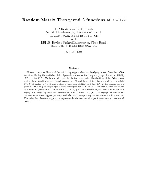
1 1 ? =X 1 ; 1 ? ps ns
1
n
(2)
=1
for Res > 1, and by an analytical continuation in the rest of the complex plane. We conjectured that the moments of (1=2 + it) high on the critical line t 2 R factor into a part which is speci c to the Riemann zeta function, and a universal component which is the corresponding moment of the characteristic polynomial Z (U; ) of matrices in U (N ), de ned with respect to an average over the CUE. The connection between N and the height T up the critical line corresponds to equating the mean density of eigenvalues N=2 with the mean density of zeros log T . This idea has subsequently been applied by Brezin and Hikami 2] to other random matrix ensembles, and by Coram and Diaconis 4] to other statistics. Our purpose here is to extend these calculations to SO(2N ) and USp(2N ), and to compare the results with what is known about the L-functions. (Only SO(2N ) is relevant, because a family

马可夫跳变系统

ISSN1751-8644continuous-884IET Control Theory Appl.,2008,Vol.2,No.10,pp.884–894 &The Institution of Engineering and Technology2008doi:10.1049/iet-cta:20070297IET Control Theory Appl.,2008,Vol.2,No.10,pp.884–894885 doi:10.1049/iet-cta:20070297&The Institution of Engineering and Technology2008886IET Control Theory Appl.,2008,Vol.2,No.10,pp.884–894&The Institution of Engineering and Technology2008doi:10.1049/iet-cta:20070297IET Control Theory Appl.,2008,Vol.2,No.10,pp.884–894887 doi:10.1049/iet-cta:20070297&The Institution of Engineering and Technology2008888IET Control Theory Appl.,2008,Vol.2,No.10,pp.884–894&The Institution of Engineering and Technology2008doi:10.1049/iet-cta:20070297IET Control Theory Appl.,2008,Vol.2,No.10,pp.884–894889 doi:10.1049/iet-cta:20070297&The Institution of Engineering and Technology2008890IET Control Theory Appl.,2008,Vol.2,No.10,pp.884–894&The Institution of Engineering and Technology2008doi:10.1049/iet-cta:20070297Figure1Behaviours of the system states in function of time t Figure2Behaviours of the system states in function of time tIET Control Theory Appl.,2008,Vol.2,No.10,pp.884–894891 doi:10.1049/iet-cta:20070297&The Institution of Engineering and Technology2008system with the computed controller is piecewise regular,impulse-free and stochastically stable.5ConclusionThis paper dealt with a class of continuous-time singular linear systems with Markovian switching.Results on stochastic stability and its robustness,and the stochastic stabilisation and its robustness are developed.The LMI framework is used to establish the different results on stability,stabilisation and their robustness.Full and partial knowledge of the jump rates are considered.The results we developed here can easily be solved using any LMI toolbox like the one of Matlab or the one of Scilab.Figure 4Behaviours of the system states in function of time tFigure 3Behaviours of the system states in function of time t892IET Control Theory Appl.,2008,Vol.2,No.10,pp.884–894&The Institution of Engineering and Technology 2008doi:10.1049/iet-cta:20070297IET Control Theory Appl.,2008,Vol.2,No.10,pp.884–894893 doi:10.1049/iet-cta:20070297&The Institution of Engineering and Technology2008894IET Control Theory Appl.,2008,Vol.2,No.10,pp.884–894&The Institution of Engineering and Technology 2008doi:10.1049/iet-cta:20070297。

Slim包使用说明说明书

Package‘slim’October14,2022Title Singular Linear Models for Longitudinal DataVersion0.1.1Description Fits singular linear models to longitudinal data.Singular linearmodels are useful when the number,or timing,of longitudinal observationsmay be informative about the observations themselves.They are describedin Farewell(2010)<doi:10.1093/biomet/asp068>,and are extensions of thelinear increments model<doi:10.1111/j.1467-9876.2007.00590.x>to generallongitudinal data.Depends R(>=3.2.0),data.table(>=1.9.6)Imports stats,MASS(>=7.3)Suggests lme4(>=1.1),jmcm(>=0.1.6.0),gee(>=4.13-19),ggplot2(>=2.1.0),testthat(>=1.0.2),knitr,rmarkdownLicense GPL-3LazyData trueRoxygenNote6.0.1VignetteBuilder knitrNeedsCompilation noAuthor Daniel Farewell[aut,cre]Maintainer Daniel Farewell<***************.uk>Repository CRANDate/Publication2017-05-1506:39:33UTCR topics documented:slim-package (2)coef.slim (2)compute_laurent (3)conﬁnt.slim (3)dialysis (4)ﬁtted.slim (5)ﬁt_slim (5)12coef.slim list_covariances (6)predict.slim (6)print.slim (7)residuals.slim (8)slim (8)slim.methods (9)summary.slim (10)vcov.slim (10)Index12 slim-package Singular linear models for longitudinal data.DescriptionThe slim packageﬁts singular linear models to longitudinal data.Singular linear models are useful when the number,or timing,of longitudinal observations may be informative about the observations themselves.They are described in Farewell(2010)<doi:10.1093/biomet/asp068>, and are extensions of the linear increments model of Diggle et al.(2007)<doi:10.1111/j.1467-9876.2007.00590.x>to general longitudinal data.DetailsThe most important function is slim,whose formula interface is similar to that of lm.See Alsoslimcoef.slim Extract Model Coefﬁcients from Singular Linear ModelDescriptionExtract Model Coefﬁcients from Singular Linear ModelUsage##S3method for class slimcoef(object,...)Argumentsobject an object of class’slim’,usually,a result of a call to’slim’....arguments passed to or from other methods.compute_laurent3 Valuea vector of model coefﬁcients.compute_laurent Laurent Expansion of Inverse of Linear Matrix FunctionDescriptionThis function computes theﬁrst two terms of the Laurent expansion of the inverse of a linear matrix function.Usagecompute_laurent(V,zapsmall=TRUE)ArgumentsV for some integer m>=1,an array of dimension(m,m,2),where V[,,1]is the intercept and V[,,2]is the slope of the linear matrix function.zapsmall logical:should zapsmall be called on the result?Default TRUE.Valuearray of dimension(m,m,2),where W[,,1]corresponds to the exponent-1,and W[,,2]corre-sponds to the exponent0.confint.slim Conﬁdence Intervals for Model Parameters from Singular LinearModelDescriptionConﬁdence Intervals for Model Parameters from Singular Linear ModelUsage##S3method for class slimconfint(object,parm,level=0.95,empirical=TRUE,...)4dialysisArgumentsobject an object of class’slim’,usually,a result of a call to’slim’.parm a speciﬁcation of which parameters are to be given conﬁdence intervals,eithera vector of numbers or a vector of names.If missing,all parameters are consid-ered.level the conﬁdence level required.empirical logical indicating if empirical variances of y should be used in estimating stan-dard errors(the default).Empirical standard errors should be used unless co-variances have been well modelled....arguments passed to or from other methods.ValueA matrix(or vector)with columns giving lower and upper conﬁdence limits for each parameter. dialysis Renal Function in Three Groups of Peritoneal Dialysis PatientsDescriptionLongitudinal data on the renal function of116patients observed on up toﬁve different occasions. UsagedialysisFormatA data.table with116rows and5variables:id patient identiﬁer,a character stringgroup treatment group identiﬁer,a character stringvintage days since starting dialysis,an integermonth month of observation,an integerrenalfn renal function of the patient at that month,numericSourceThis data is derived from the Global Fluid Study.This part of the study was led by Dr James Chess and Prof.Nick Topley.ReferencesLambie,M.,Chess,J.et al.(2013).Independent effects of systemic and peritoneal inﬂammation on peritoneal dialysis survival.J Am Soc Nephrol,24,2071–80.ﬁtted.slim5 fitted.slim Extract Model Fitted Values from Singular Linear ModelDescriptionExtract Model Fitted Values from Singular Linear ModelUsage##S3method for class slimfitted(object,...)Argumentsobject an object of class’slim’,usually,a result of a call to’slim’....arguments passed to or from other methods.Valuea vector ofﬁtted values from the modelﬁt.fit_slim Fitter Function for Singular Linear ModelsDescriptionThis function computes the limiting solution to the estimating equation sum(x’V^-1(y-x beta))= 0as the covariance V tends from V[,,1]+V[,,2]to V[,,1].Usagefit_slim(x,V,y)Argumentsx list of design matrices,one for each subject,all having the same number of columns.V list of covariance arrays,one for each subject,matching the dimensions of y.y list of response vectors,one for each subject.Valuea list with components coefﬁcients(the limiting solution),residuals,ﬁtted_values,vcov_empiricaland vcov_modelled.6predict.slim list_covariances List Covariance Matrices for Every SubjectDescriptionThis function is generic,and methods exists for character,list,function,and various modelﬁt classes.Usagelist_covariances(obj,t)##S3method for class characterlist_covariances(obj,t)##S3method for class listlist_covariances(obj,t)##S3method for class functionlist_covariances(obj,t)##S3method for class jmcmModlist_covariances(obj,t)##S3method for class lmerModlist_covariances(obj,t)Argumentsobj an R object of class character,function,or a modelﬁtt list of vectors of observation times,one for each subjectValuea list containing covariance matrices of appropriate dimensionspredict.slim Model Predictions from Singular Linear ModelDescriptionModel Predictions from Singular Linear Modelprint.slim7Usage##S3method for class slimpredict(object,newdata,...)Argumentsobject an object of class’slim’,usually,a result of a call to’slim’.newdata An optional data frame in which to look for variables with which to predict.If omitted,theﬁtted values are used....arguments passed to or from other methods.Valuea vector of model predictions.print.slim Print’slim’ObjectsDescription’print’methods for class’slim’and’slim_summary’.’print.slim_summary’differs only in its de-fault value of’empirical’.Usage##S3method for class slimprint(x,empirical=TRUE,digits=max(3,getOption("digits")-3),signif.stars=getOption("show.signif.stars"),...)##S3method for class slim_summaryprint(x,empirical=x$empirical,...)Argumentsx an object of class’slim’or’slim_summary’,as appropriate.empirical logical indicating if empirical variances of y should be used in estimating stan-dard errors(the default).Empirical standard errors should be used unless co-variances have been well modelled.digits minimal number of signiﬁcant digits,see print.default.signif.stars logical.If TRUE,‘signiﬁcance stars’are printed for each coefﬁcient....arguments passed to or from other methods.Valuex,invisibly.8slim residuals.slim Extract Model Residuals from Singular Linear ModelDescriptionExtract Model Residuals from Singular Linear ModelUsage##S3method for class slimresiduals(object,...)Argumentsobject an object of class’slim’,usually,a result of a call to’slim’....arguments passed to or from other methods.Valuea vector of model residuals.slim Fit Singular Linear ModelsDescriptionFit a singular linear model to longitudinal data.Usageslim(formula,data,covariance="randomwalk",limit=~1,contrasts=NULL)Argumentsformula a model formula for theﬁxed effectsdata a’data.table’with two keys,respectively identifying subjects and observation timescovariance an R object for which a’list_covariances’method exists.Options include a character string such as"identity","randomwalk"(the default),"brownian"or"pascal";a list of covariance matrices;a function to be used in’outer’and ap-plied to the observation times;or a’jmcmMod’or’lmerMod’modelﬁt.limit a one-sided model formula for the(thin)Cholesky factor of the limiting covari-ance matrix(default~1,so the limiting covariance matrix is the matrix of ones) contrasts an optional list.See the’contrasts.arg’argument of’model.matrix.default’.slim.methods9 Valuean object of class’slim’Examplesslim_fit<-slim(renalfn~group+month,dialysis)summary(slim_fit)if(require("lme4")){lmer_fit<-lmer(renalfn~group+month+(1+month|id),dialysis)slim_fit<-slim(renalfn~1+group+month,dialysis,covariance=lmer_fit)summary(slim_fit)summary(slim_fit,empirical=FALSE)}if(require("jmcm")){jmcm_fit<-jmcm(renalfn|id|month~group|1,dialysis,triple=rep(2L,3),cov.method="mcd")slim_fit<-slim(renalfn~group+month,dialysis,covariance=jmcm_fit)summary(slim_fit)summary(slim_fit,empirical=FALSE)}slim.methods Methods for Singular Linear Model FitsDescriptionMethods for Singular Linear Model FitsArgumentsobject an object of class’slim’,usually,a result of a call to’slim’.empirical logical indicating if empirical variances of y should be used in estimating stan-dard errors(the default).Empirical standard errors should be used unless co-variances have been well modelled....arguments passed to or from other methods.10vcov.slim summary.slim Summarizing Singular Linear Model FitsDescription’summary’method for class’slim’.Usage##S3method for class slimsummary(object,empirical=TRUE,...)Argumentsobject an object of class’slim’,usually,a result of a call to’slim’.empirical logical indicating if empirical variances of y should be used in estimating stan-dard errors(the default).Empirical standard errors should be used unless co-variances have been well modelled....arguments passed to or from other methods.Valuean object with class c("slim_summary","slim")and,in addition to the usual’slim’components, coefﬁcient_matrix(the matrix of estimated coefﬁcients,standard errors,z-and p-values)and em-pirical(logical indicating if empirical standard errors have been used)vcov.slim Extract Variance-Covariance Matrix from a’slim’ObjectDescription’vcov’method for class’slim’.Usage##S3method for class slimvcov(object,empirical=TRUE,...)Argumentsobject an object of class’slim’,usually,a result of a call to’slim’.empirical logical indicating if empirical variances of y should be used in estimating stan-dard errors(the default).Empirical standard errors should be used unless co-variances have been well modelled....arguments passed to or from other methods.vcov.slim11Valuea matrix of the estimated covariances between the parameter estimates.Index∗datasetsdialysis,4coef.slim,2compute_laurent,3confint.slim,3dialysis,4fit_slim,5fitted.slim,5list_covariances,6predict.slim,6print.default,7print.slim,7print.slim_summary(print.slim),7 residuals.slim,8slim,2,8slim-package,2slim.methods,9summary.slim,10vcov.slim,1012。

《机械振动》常用英语词汇

机械振动常用英语词汇表Aacceleration 加速度accelerometer加速度计algebraic 代数的amplitude 振幅，幅度，幅值amplitude-frequency characteristics 幅频特性amplitude-frequency curve幅频特性曲线amplitude spectrum 幅值谱angular velocity 角速度aperiodic 非周期的average value 均值axis 轴，轴线，坐标轴Bbeam 梁beating 拍boundary condition 边界条件Ccantilever 悬臂centrifugal 离心的centrifugal force 离心力characteristic determinant特征行列式characteristic equation 特征方程characteristic matrix 特征矩阵circular frequency 圆频率clamped 固支的clamped-hinged 固支-铰支的clockwise 顺时针的coefficient系数column matrix 列矩阵condition monitoring 状态监测converge 收敛converged 收敛的convolution 卷曲，卷积convolution integral 卷积积分column 列coordinate 坐标coulomb damping 库仑阻尼counterclockwise 逆时针的coupling 耦合critical speed 临界转速critically damped 临界阻尼的Ddamper 阻尼器damped free vibration有阻尼自由振动damped natural frequency有阻尼固有频率damping 阻尼damping factor 阻尼系数damping ratio 阻尼比decay 衰减deflection 位移，挠度degree of freedom 自由度denominator 分母density 密度derivative 导数determinant 行列式diagonal matrix 对角矩阵differential 微分的dimensionless 无量纲的discrete 离散的disk 盘displacement 位移dissipate 耗散divide 除DOF (degree of freedom) 自由度Duhamel’s Integral杜哈美积分Dunkerley’s method 邓克利法dynamic coupling 动力耦合dynamic matrix 动力矩阵Eeccentric mass 偏心质量eccentricity 偏心距effective mass有效质量effective value，RMS value 有效值eigenvalue 特征值eigenvector 特征向量elastic body 弹性体element 元素，单元equilibrium 平衡equivalent viscous damping等效粘性阻尼exponential 指数的FFast Fourier Transform快速傅立叶变换factorize 分解因式flexibility 柔度flexibility matrix 柔度矩阵forced harmonic vibration强迫简谐振动forced vibration 强迫振动Fourier series傅里叶级数Fourier transform傅立叶变换free vibration自由振动free response自由响应frequency ratio频率比fundamental frequency 基频fundamental frequency vibration基频振动fundamental mode 第一阶模态Ggeneral solution 通解generalized coordinates 广义坐标generalized force 广义力generalized mass 广义质量generalized stiffness 广义刚度gravitational force 重力Hharmonic 简谐的harmonic force 简谐激振力harmonic motion 简谐运动homogeneous 齐次的homogeneous equation 齐次方程Hooke’s law 虎克定律Iidentity matrix 单位矩阵impulse excitation 冲击激励impulse response function冲击响应函数independent coordinate 独立坐标inertia force, inertial force 惯性力initial condition 初始条件initial phase 初相位integral 积分的inverse matrix 逆矩阵iteration 迭代Kkinetic energy 动能Llinear 线性的logarithm 对数logarithmic decrement 对数衰减率longitudinal 纵向的lumped mass 集中质量Mmass matrix 质量矩阵matrix iteration 矩阵迭代法modal coordinates 模态坐标modal damping ratio 模态阻尼比modal mass 模态质量modal matrix 模态矩阵，振型矩阵modal stiffness 模态刚度modal testing 模态试验mode shape 振型（模态）modulus of elasticity 弹性模量moment 弯矩multi-degree-of- freedom system 多自由度系统multiply 乘Nnatural frequency 固有频率natural logarithm 自然对数nondimensional 无量纲的normal force 法向力normalization 正则化normal mode 主振型numerator （分数的）分子Ooff-diagonal element非对角元素orthogonal 正交的orthogonality 正交性orthonormal mode 正则振型oscillatory 振动的，摆动的oscillatory motion 振荡运动overdamped 过阻尼的Pparallel 并联，平行partial differential 偏微分particular solution 特解peak value 峰值pendulum (钟）摆periodic 周期的periodic motion 周期运动phase 相位phase frequency characteristics 相频特性phase frequency curve相频特性曲线polar moment of inertia极转动惯量polynomial 多项式potential energy 势能power 幂（乘方），功率premultiply 左乘，前乘principal coordinate 主坐标principal frequency 主频率principal mass 主质量principal vibration 主振动principal stiffness 主刚度principle of superposition叠加原理product 乘积pulse excitation 脉冲激励Qquasi-periodic vibration准周期振动quotient 商R radian 弧度random vibration 随机振动Rayleigh method 瑞利法Rayleigh quotient 瑞利商Rayleigh-Ritz Method瑞利-里兹法real symmetric matrix 实对称矩阵reciprocal 倒数的，倒数recurrence formula递推公式, 循环resolution 分辨率resonance 共振rigid body 刚体rms 均方根rod 杆root mean square 均方根root solving 求根rotating machine 旋转机械rotor 转子rotor-support system转子支承系统row 行row matrix 行矩阵Sself-excited vibration 自激振动series 串联shaft 轴shaft vibration 轴振动shear 剪力shear modulus of elasticity剪切弹性模量shock excitation 冲击激励shock isolation 振动隔离shock response 冲击响应SI (International System of Units)国际（单位）制simply supported 简支的singular matrix 奇异矩阵single-DOF 单自由度slope 转角，斜率spin 旋转spring 弹簧square root 平方根state vector 状态向量static coupling 静力耦合static equilibrium position静平衡位置steady state 稳态step function 阶跃函数stiffness 刚度stiffness influence coefficient刚度影响系数stiffness matrix 刚度矩阵strain 应变stress 应力structural damping 结构阻尼subscript 下标successive 接连不断的support motion 支承运动symmetric matrix 对称矩阵Ttangent 切线，正切tangential 切向的tensile 拉力的，张力的tension 张力，拉力terminology 术语torque 扭矩, 转矩torsion 扭转torsional 扭转的torsional stiffness 抗扭刚度torsional vibration扭转振动TR (transmissibility) 传递率,trace of the matrix 矩阵的迹transfer matrix method传递矩阵法transient response 瞬态响应transient vibration 瞬态振动transmissibility 隔振系数transpose 转置trial 测试，试验triangular matrix 三角矩阵truncation error截断误差，舍位误差twist 扭，转Uunbalance 不平衡unbalance response 不平衡响应underdamped 欠阻尼的unit impulse 单位脉冲unit matrix 单位矩阵unit vector 单位向量unsymmetric 非对称upper triangular matrix 上三角阵Vvelocity 速度vertical vibration 垂直振动vibration 振动vibration absorber 吸振器vibration isolation 隔振viscous damping 粘性阻尼。

随机矩阵理论及其统计应用

随机矩阵理论及其统计应用Title: Random Matrix Theory and Its Statistical ApplicationsIntroduction:Random Matrix Theory (RMT) is a branch of mathematics that studies the properties and characteristics of matrices with randomly distributed elements. Initially developed in the mid-20th century to model nuclear energy levels, RMT has found extensive applications in various scientific fields, including physics, finance, and computer science. In this article, we will explore the basics of RMT, its statistical applications, and the significance it holds in understanding complex systems.1. Random Matrix Theory FundamentalsRandom matrices are defined as matrices whose elements are generated from a probability distribution. The properties and statistics of these matrices differ from those of deterministic matrices, leading to unique mathematical characteristics. Key concepts in RMT include:1.1 UniversalityRandom matrices exhibit universal behavior, meaning that certain statistical properties are independent of the specific distribution used to generate the matrix elements. This universality enables the application of RMT beyond specific systems, making it a powerful tool for understanding complex phenomena.1.2 EnsemblesRMT classifies random matrices into different ensembles based on their symmetry properties. The most commonly studied ensembles are the Gaussian ensembles (GOE, GUE, and GSE), characterized by their symmetries and probability distributions. Each ensemble has distinct statistical properties and is utilized to model different physical or financial systems.2. Statistical Applications of Random Matrix Theory2.1 Quantum ChaosRandom Matrix Theory plays a crucial role in understanding quantum chaotic systems. By analyzing statistical properties of random matrices, RMT provides insights into the energy levels and spectral statistics of chaotic quantum systems, such as atoms, nuclei, and even quantum billiards. RMT has successfully explained the universal behavior observed experimentally in these systems.2.2 Financial MarketsThe complex dynamics of financial markets have attracted the application of RMT. By considering financial returns as random variables, RMT enables the analysis of correlations, volatility, and risk in financial time series. RMT-based methods have been applied to portfolio optimization, risk management, and financial forecast modeling.2.3 Wireless Communication SystemsRandom Matrix Theory has also found applications in wireless communication systems. Analysis of the random matrices formed by the correlation matrix of received signals helps in understanding multi-antennasystems, improving signal detection algorithms, and enhancing system capacity.3. The Significance and Limitations of Random Matrix TheoryRMT has been successful in providing powerful analytical tools to understand complex systems in various fields. Its universality and applicability make it a valuable approach for statistical analysis. However, there are certain limitations to consider:3.1 System-Specific EffectsDespite universality, RMT may not capture all the system-specific characteristics that determine the behavior of a given complex system. Therefore, careful consideration and adaptation of RMT principles are required based on specific applications.3.2 Computational ChallengesComputational complexity can pose challenges in applying RMT to large-scale systems. The calculation of eigenvalues and eigenvectors of large random matrices can be time-consuming and computationally intensive, requiring efficient algorithms and modern computational resources.Conclusion:Random Matrix Theory has emerged as a powerful mathematical tool for understanding complex systems and analyzing statistical properties. Its applications in fields like quantum physics, finance, and wireless communications demonstrate its versatility and broad impact. Despite limitations, RMT continues to evolve, providing valuable insights into adiverse range of phenomena and contributing to advancements in statistical analysis techniques.。

矩阵集中不等式MATRIX CONCENTRATION INEQUALITIES

MATRIX CONCENTRATION INEQUALITIES VIA THE METHOD OF EXCHANGEABLE PAIRS
LESTER MACKEY AND MICHAEL I. JORDAN∗ RICHARD Y. CHEN, BRENDAN FARRELL, AND JOEL A. TROPP†
This paper is based on two independent manuscripts from mid-2011 that both applied the method of exchangeable pairs to establish matrix concentration inequalities. One manuscript is by Mackey and Jordan; the other is by Chen, Farrell, and Tropp. The authors have combined this research into a single uniﬁed presentation, with equal contributions from both groups. 1. Introduction Matrix concentration inequalities control the ﬂuctuations of a random matrix about its mean. At present, these results provide an eﬀective method for studying sums of independent random matrices and matrix martingales [Oli09, Tro11a, Tro11b, HKZ11]. They have been used to streamline the analysis of structured random matrices in a range of applications, including statistical estimation [Kol11], randomized linear algebra [Git11, CD11b], stability of least-squares approximation [CDL11], combinatorial and robust optimization [So11, CSW11], matrix completion [Gro11, Rec11, MTJ11], and random graph theory [Oli09]. These works comprise only a small sample of the papers that rely on matrix concentration inequalities. Nevertheless, it remains common to encounter new classes of random matrices that we cannot treat with the available techniques. The purpose of this paper is to lay the foundations of a new approach for analyzing structured random matrices. Our work is based on Chatterjee’s technique for developing scalar concentration inequalities [Cha07, Cha08] via Stein’s method of exchangeable pairs [Ste72]. We extend this argument to the matrix setting, where we use it to establish exponential concentration results (Theorems 4.1 and 5.1) and polynomial moment inequalities (Theorem 7.1) for the spectral norm of a random matrix. To illustrate the power of this idea, we show that our general results imply several important concentration bounds for a sum of independent, random, Hermitian matrices [LPP91, JX03, Tro11b]. We obtain a matrix Hoeﬀding inequality with optimal constants (Corollary 4.2) and a version of the matrix Bernstein inequality (Corollary 5.2). Our techniques also yield concise proofs of the matrix Khintchine inequality (Corollary 7.4) and the matrix Rosenthal inequality (Corollary 7.5). The method of exchangeable pairs also applies to matrices constructed from dependent random variables. We oﬀer a hint of the prospects by establishing concentration results for several other

random-matrices

Random MatricesA random matrix is a matrix whose entries are random variables.The moments of an n×n random matrix A are the expected values of the random variablestr(A k).This project asks you toﬁrst investigate the moments of families of random matrices,especially limiting behavior as n→∞.Here is an interesting family of square random matrices.Take an n×n random matrix M whose entries are normally distributed random variables with mean0and constant variance a,and form A=(M+M T)/2.Preliminary question:what are the means and variances of the entries in A?It’s worthwhile thinking through what the mean and variance of the random variables tr(A k)are for small n,but the fun begins when n grows large.The constant a will have to be allowed to vary with n in order to obtain limiting values of E[tr(A k)]which are neither zero nor inﬁnite.Write a n for the value you use for the n×n case.Investigate the resulting limiting values.Can you account for whatever patterns you observe?There is a close relationship between traces and eigenvalues.Investigate the limiting distribution of eigenvalues of these random matrices A as n grows large.There are many other directions in which this kind of exploration can be pursued.For example,what happens if you use diﬀerent random variables for the entries in A—perhaps not even normally distributed?The oﬀdiagonal entries are independent and identically distributed;what happens if we alter those assumptions?And there are many families of matrices other than symmetric ones,as well.Resources:We recommend the use of MATLAB for this project.We can also recommend the18.440textbook A First Course in Probability by Sheldon Ross.。

rWishart包用户手册说明书

Package‘rWishart’October14,2022Title Random Wishart Matrix GenerationVersion0.1.2Maintainer Ben Barnard<**********************>Description An expansion of R's'stats'random wishart matrix generation.This package allows the user to generate singular,Uhlig and Harald(1994)<doi:10.1214/aos/1176325375>,and pseudo wishart,Diaz-Garcia,et al.(1997)<doi:10.1006/jmva.1997.1689>,matrices.In addition the user can generatewishart matrices with fractional degrees of freedom,Adhikari(2008)<doi:10.1061/(ASCE)0733-9399(2008)134:12(1029)>,commonly used in volatilityers can also use this package to create random covariance matrices.Depends R(>=3.3)Imports Matrix,MASS,stats,lazyevalLicense GPL-2Encoding UTF-8LazyData trueRoxygenNote6.1.1Suggests covr,knitr,rmarkdown,testthatURL https://NeedsCompilation noAuthor Ben Barnard[aut,cre],Dean Young[aut]Repository CRANDate/Publication2019-11-1923:10:02UTCR topics documented:rFractionalWishart (2)rNonsingularWishart (3)rPsuedoWishart (4)rSingularWishart (5)rWishart (6)wishartTest (7)12rFractionalWishart Index8 rFractionalWishart Random Fractional Wishart MatrixDescriptionGenerate n random matrices,distributed according to the Wishart distribution with parameters Sigma and df,W_p(Sigma,df).UsagerFractionalWishart(n,df,Sigma,covariance=FALSE,simplify="array")Argumentsn integer:the number of replications.df numeric parameter,“degrees of freedom”.Sigma positive deﬁnite(p×p)“scale”matrix,the matrix parameter of the distribution.covariance logical on whether a covariance matrix should be generatedsimplify logical or character string;should the result be simpliﬁed to a vector,matrix or higher dimensional array if possible?For sapply it must be named andnot abbreviated.The default value,TRUE,returns a vector or matrix if appro-priate,whereas if simplify="array"the result may be an array of“rank”(=length(dim(.)))one higher than the result of FUN(X[[i]]).DetailsIf X_1,...,X_m is a sample of m independent multivariate Gaussians with mean vector0,and covariance matrix Sigma,the distribution of M=X’X is W_p(Sigma,m).ValueA numeric array of dimension p*p*n,where each array is a positive semideﬁnite matrix,a real-ization of the Wishart distribution W_p(Sigma,df)ReferencesAdhikari,S.(2008).Wishart random matrices in probabilistic structural mechanics.Journal of engineering mechanics,134(12),doi:10.1061/(ASCE)07339399(2008)134:12(1029). ExamplesrFractionalWishart(2,22.5,diag(1,20))rNonsingularWishart3 rNonsingularWishart Random Nonsingular Wishart MatrixDescriptionGenerate n random matrices,distributed according to the Wishart distribution with parameters Sigma and df,W_p(Sigma,df).UsagerNonsingularWishart(n,df,Sigma,covariance=FALSE,simplify="array")Argumentsn integer:the number of replications.df numeric parameter,“degrees of freedom”.Sigma positive deﬁnite(p×p)“scale”matrix,the matrix parameter of the distribution.covariance logical on whether a covariance matrix should be generatedsimplify logical or character string;should the result be simpliﬁed to a vector,matrix or higher dimensional array if possible?For sapply it must be named andnot abbreviated.The default value,TRUE,returns a vector or matrix if appro-priate,whereas if simplify="array"the result may be an array of“rank”(=length(dim(.)))one higher than the result of FUN(X[[i]]).DetailsIf X_1,...,X_m is a sample of m independent multivariate Gaussians with mean vector0,and covariance matrix Sigma,the distribution of M=X’X is W_p(Sigma,m).ValueA numeric array of dimension p*p*n,where each array is a positive semideﬁnite matrix,a real-ization of the Wishart distribution W_p(Sigma,df)ExamplesrNonsingularWishart(2,20,diag(1,5))4rPsuedoWishart rPsuedoWishart Random Psuedo Wishart MatrixDescriptionGenerate n random matrices,distributed according to the Wishart distribution with parameters Sigma and df,W_p(Sigma,df).UsagerPsuedoWishart(n,df,Sigma,covariance=FALSE,simplify="array")Argumentsn integer:the number of replications.df numeric parameter,“degrees of freedom”.Sigma positive deﬁnite(p×p)“scale”matrix,the matrix parameter of the distribution.covariance logical on whether a covariance matrix should be generatedsimplify logical or character string;should the result be simpliﬁed to a vector,matrix or higher dimensional array if possible?For sapply it must be named andnot abbreviated.The default value,TRUE,returns a vector or matrix if appro-priate,whereas if simplify="array"the result may be an array of“rank”(=length(dim(.)))one higher than the result of FUN(X[[i]]).DetailsIf X_1,...,X_m is a sample of m independent multivariate Gaussians with mean vector0,and covariance matrix Sigma,the distribution of M=X’X is W_p(Sigma,m).ValueA numeric array of dimension p*p*n,where each array is a positive semideﬁnite matrix,a real-ization of the Wishart distribution W_p(Sigma,df)ReferencesDiaz-Garcia,Jose A,Ramon Gutierrez Jaimez,and Kanti V Mardia.1997.“Wishart and Pseudo-Wishart Distributions and Some Applications to Shape Theory.”Journal of Multivariate Analysis 63(1):73–87.doi:10.1006/jmva.1997.1689.ExamplesrPsuedoWishart(2,5,diag(1,20))rSingularWishart5 rSingularWishart Random Singular Wishart MatrixDescriptionGenerate n random matrices,distributed according to the Wishart distribution with parameters Sigma and df,W_p(Sigma,df).UsagerSingularWishart(n,df,Sigma,covariance=FALSE,simplify="array")Argumentsn integer:the number of replications.df numeric parameter,“degrees of freedom”.Sigma positive deﬁnite(p×p)“scale”matrix,the matrix parameter of the distribution.covariance logical on whether a covariance matrix should be generatedsimplify logical or character string;should the result be simpliﬁed to a vector,matrix or higher dimensional array if possible?For sapply it must be named andnot abbreviated.The default value,TRUE,returns a vector or matrix if appro-priate,whereas if simplify="array"the result may be an array of“rank”(=length(dim(.)))one higher than the result of FUN(X[[i]]).DetailsIf X_1,...,X_m is a sample of m independent multivariate Gaussians with mean vector0,and covariance matrix Sigma,the distribution of M=X’X is W_p(Sigma,m).ValueA numeric array of dimension p*p*n,where each array is a positive semideﬁnite matrix,a real-ization of the Wishart distribution W_p(Sigma,df)ReferencesUhlig,Harald.1994.“On Singular Wishart and Singular Multivariate Beta Distributions.”The Annals of Statistics22(1):395–405.doi:10.1214/aos/1176325375.ExamplesrSingularWishart(2,5,diag(1,20))6rWishart rWishart Random Wishart Matrix GenerationDescriptionAn expansion of R’s’stats’random wishart matrix generation.This package allows the user to gen-erate singular,Uhlig and Harald(1994)<doi:10.1214/aos/1176325375>,and pseudo wishart,Diaz-Garcia,et al.(1997)<doi:10.1006/jmva.1997.1689>,matrices.In addition the user can generate wishart matrices with fractional degrees of freedom,Adhikari(2008)<doi:10.1061/(ASCE)0733-9399(2008)134:12(1029)>,commonly used in volatility ers can also use this package to create random covariance matrices.Generate n random matrices,distributed according to the Wishart distribution with parameters Sigma and df,W_p(Sigma,df).UsagerWishart(n,df,Sigma,covariance=FALSE,simplify="array")Argumentsn integer:the number of replications.df numeric parameter,“degrees of freedom”.Sigma positive deﬁnite(p×p)“scale”matrix,the matrix parameter of the distribution.covariance logical on whether a covariance matrix should be generatedsimplify logical or character string;should the result be simpliﬁed to a vector,matrix or higher dimensional array if possible?For sapply it must be named andnot abbreviated.The default value,TRUE,returns a vector or matrix if appro-priate,whereas if simplify="array"the result may be an array of“rank”(=length(dim(.)))one higher than the result of FUN(X[[i]]).DetailsIf X_1,...,X_m is a sample of m independent multivariate Gaussians with mean vector0,and covariance matrix Sigma,the distribution of M=X’X is W_p(Sigma,m).ValueA numeric array of dimension p*p*n,where each array is a positive semideﬁnite matrix,a real-ization of the Wishart distribution W_p(Sigma,df)ExamplesrWishart(2,5,diag(1,20))wishartTest7 wishartTest Test if Matrix is a Wishart MatrixDescriptionGiven a random Wishart matrix,B,from W_p(Sigma,df)and independent random vector a,then (a’B a)/(a’Sigma a)is chi-squared with df degrees of freedom.UsagewishartTest(WishMat,Sigma,vec=NULL)ArgumentsWishMat random Wishart Matrix from W_p(Sigma,df)Sigma Covariance matrix for W_p(Sigma,df)vec independent random vectorValueA chi-squared random variable with df degrees of freedom.ExampleswishartTest(rWishart(1,5,diag(1,20),simplify=FALSE)[[1]],diag(1,20))Indexarray,2–6rFractionalWishart,2 rNonsingularWishart,3rPsuedoWishart,4rSingularWishart,5rWishart,6rWishart-package(rWishart),6wishartTest,78。

随机矩阵奇异值分解算法在3D重建中的应用效果评估

随机矩阵奇异值分解算法在3D重建中的应用效果评估随着科学技术的进步和计算机图形学的快速发展，三维重建技术在各个领域得到了广泛的应用。

其中，随机矩阵奇异值分解算法作为一种常用的三维重建算法，其在提高重建效果方面具有很大的潜力。

本文将对随机矩阵奇异值分解算法在3D重建中的应用效果进行评估。

一、随机矩阵奇异值分解算法简介随机矩阵奇异值分解算法（Random Matrix Singular Value Decomposition, RMSVD）是一种基于奇异值分解（Singular Value Decomposition, SVD）的重建算法，其核心思想是通过矩阵分解的方式来还原三维模型的形状和纹理信息。

相比于其他算法，随机矩阵奇异值分解算法具有快速、准确等特点，被广泛应用于三维重建领域。

二、随机矩阵奇异值分解算法在3D重建中的应用效果评估为了评估随机矩阵奇异值分解算法在3D重建中的应用效果，我们进行了一系列的实验。

首先，我们收集了一批包含不同形状和纹理的三维模型作为测试数据集。

然后，利用随机矩阵奇异值分解算法对这些三维模型进行了重建，并对重建结果进行了评估。

在评估指标方面，我们采用了两种常用的指标：均方根误差（Root Mean Square Error, RMSE）和结构相似性指数（Structural Similarity Index, SSIM）。

RMSE用于评估重建模型与原始模型之间的几何误差，而SSIM则用于评估重建模型与原始模型之间的纹理相似性。

通过对比不同算法的评估结果，我们可以客观地评估随机矩阵奇异值分解算法在3D重建中的应用效果。

实验结果表明，随机矩阵奇异值分解算法在3D重建中取得了较好的效果。

通过与其他重建算法的比较，我们发现随机矩阵奇异值分解算法在几何误差和纹理相似性方面均能取得较佳的结果。

具体而言，随机矩阵奇异值分解算法在几何误差方面的均方根误差较小，说明其能够较准确地还原原始模型的形状信息；同时，在纹理相似性方面的结构相似性指数较高，说明其能够较好地还原原始模型的纹理信息。

Tikhonov吉洪诺夫正则化

Tikhonov regularizationFrom Wikipedia, the free encyclopediaTikhonov regularization is the most commonly used method of of named for . In , the method is also known as ridge regression . It is related to the for problems.The standard approach to solve an of given as,b Ax =is known as and seeks to minimize the2bAx -where •is the . However, the matrix A may be or yielding a non-unique solution. In order to give preference to a particular solution with desirable properties, the regularization term is included in this minimization:22xb Ax Γ+-for some suitably chosen Tikhonov matrix , Γ. In many cases, this matrix is chosen as the Γ= I , giving preference to solutions with smaller norms. In other cases, operators ., a or a weighted ) may be used to enforce smoothness if the underlying vector is believed to be mostly continuous. This regularizationimproves the conditioning of the problem, thus enabling a numerical solution. An explicit solution, denoted by , is given by:()b A A A xTTT 1ˆ-ΓΓ+=The effect of regularization may be varied via the scale of matrix Γ. For Γ=αI , when α = 0 this reduces to the unregularized least squares solution providedthat (A T A)−1 exists.Contents••••••••Bayesian interpretationAlthough at first the choice of the solution to this regularized problem may look artificial, and indeed the matrix Γseems rather arbitrary, the process can be justified from a . Note that for an ill-posed problem one must necessarily introduce some additional assumptions in order to get a stable solution.Statistically we might assume that we know that x is a random variable with a . For simplicity we take the mean to be zero and assume that each component isindependent with σx. Our data is also subject to errors, and we take the errorsin b to be also with zero mean and standard deviation σb. Under these assumptions the Tikhonov-regularized solution is the solution given the dataand the a priori distribution of x, according to . The Tikhonov matrix is then Γ=αI for Tikhonov factor α = σb/ σx.If the assumption of is replaced by assumptions of and uncorrelatedness of , and still assume zero mean, then the entails that the solution is minimal . Generalized Tikhonov regularizationFor general multivariate normal distributions for x and the data error, one can apply a transformation of the variables to reduce to the case above. Equivalently,one can seek an x to minimize22Q P x x b Ax -+-where we have used 2P x to stand for the weighted norm x T Px (cf. the ). In the Bayesian interpretation P is the inverse of b , x 0 is the of x , and Q is the inverse covariance matrix of x . The Tikhonov matrix is then given as a factorization of the matrix Q = ΓT Γ. the ), and is considered a . This generalized problem can be solved explicitly using the formula()()010Ax b P A QPA A x T T-++-[] Regularization in Hilbert spaceTypically discrete linear ill-conditioned problems result as discretization of , and one can formulate Tikhonov regularization in the original infinite dimensional context. In the above we can interpret A as a on , and x and b as elements in the domain and range of A . The operator ΓΓ+T A A *is then a bounded invertible operator.Relation to singular value decomposition and Wiener filterWith Γ= αI , this least squares solution can be analyzed in a special way viathe . Given the singular value decomposition of AT V U A ∑=with singular values σi , the Tikhonov regularized solution can be expressed asb VDU xT =ˆ where D has diagonal values22ασσ+=i i ii Dand is zero elsewhere. This demonstrates the effect of the Tikhonov parameteron the of the regularized problem. For the generalized case a similar representation can be derived using a . Finally, it is related to the :∑==qi iiT i i v bu f x1ˆσwhere the Wiener weights are 222ασσ+=i i i f and q is the of A .Determination of the Tikhonov factorThe optimal regularization parameter α is usually unknown and often in practical problems is determined by an ad hoc method. A possible approach relies on the Bayesian interpretation described above. Other approaches include the , , , and . proved that the optimal parameter, in the sense of minimizes:()()[]21222ˆTTXIX XX I Tr y X RSSG -+--==αβτwhereis the and τ is the effective number .Using the previous SVD decomposition, we can simplify the above expression:()()21'22221'∑∑==++-=qi iiiqi iiub u ub u y RSS ασα()21'2220∑=++=qi iiiub u RSS RSS ασαand∑∑==++-=+-=qi iqi i i q m m 12221222ασαασστRelation to probabilistic formulationThe probabilistic formulation of an introduces (when all uncertainties are Gaussian) a covariance matrix C M representing the a priori uncertainties on the model parameters, and a covariance matrix C D representing the uncertainties on the observed parameters (see, for instance, Tarantola, 2004 ). In the special case when these two matrices are diagonal and isotropic,and, and, in this case, the equations of inverse theory reduce to theequations above, with α = σD / σM .HistoryTikhonov regularization has been invented independently in many differentcontexts. It became widely known from its application to integral equations from the work of and D. L. Phillips. Some authors use the term Tikhonov-Phillips regularization . The finite dimensional case was expounded by A. E. Hoerl, who took a statistical approach, and by M. Foster, who interpreted this method as a - filter. Following Hoerl, it is known in the statistical literature as ridge regression .[] References•(1943). "Об устойчивости обратных задач [On the stability of inverse problems]". 39 (5): 195–198.•Tychonoff, A. N. (1963). "О решении некорректно поставленных задач и методе регуляризации [Solution of incorrectly formulated problems and the regularization method]". Doklady Akademii Nauk SSSR151:501–504.. Translated in Soviet Mathematics4: 1035–1038. •Tychonoff, A. N.; V. Y. Arsenin (1977). Solution of Ill-posed Problems.Washington: Winston & Sons. .•Hansen, ., 1998, Rank-deficient and Discrete ill-posed problems, SIAM •Hoerl AE, 1962, Application of ridge analysis to regression problems, Chemical Engineering Progress, 58, 54-59.•Foster M, 1961, An application of the Wiener-Kolmogorov smoothing theory to matrix inversion, J. SIAM, 9, 387-392•Phillips DL, 1962, A technique for the numerical solution of certain integral equations of the first kind, J Assoc Comput Mach, 9, 84-97•Tarantola A, 2004, Inverse Problem Theory (), Society for Industrial and Applied Mathematics,•Wahba, G, 1990, Spline Models for Observational Data, Society for Industrial and Applied Mathematics。

复对称矩阵的合同标准形

复对称矩阵的合同标准形A symmetric matrix is a square matrix that is equal to its transpose. In other words, a matrix A is symmetric if A = A^T. For a complex symmetric matrix, it must satisfy the condition that its conjugate transpose is equal to itself, , A = A^H.这意味着对于一个复对称矩阵，它必须满足其共轭转置等于其本身的条件，即A=A^H。

When it comes to the congruent standard form of a complex symmetric matrix, it involves transforming it into a simpler, standard form through a congruence transformation. This transformation involves multiplying the matrix by a non-singular matrix on both sides, , M^TAM, where M is a non-singular matrix.谈到复对称矩阵的合同标准形，它涉及通过合同变换将其转化为更简单的标准形式。

这种转换涉及在两侧用非奇异矩阵乘以该矩阵，即M^TAM，其中M是一个非奇异矩阵。

The congruent standard form of a complex symmetric matrix is important in various mathematical and scientific applications. It allows for easier analysis and manipulation of the matrix, making it more amenable to mathematical operations and calculations.复对称矩阵的合同标准形在各种数学和科学应用中非常重要。

随机矩阵奇异值分解算法在语义分析中的应用效果评估

随机矩阵奇异值分解算法在语义分析中的应用效果评估随机矩阵奇异值分解（randomized matrix singular value decomposition，简称RSVD）算法是一种用于数据降维和特征提取的方法，近年来在语义分析领域中得到了广泛的应用。

本文将评估随机矩阵奇异值分解算法在语义分析中的应用效果，探讨其在准确性、效率性以及可扩展性等方面的优势。

1. 算法原理与步骤随机矩阵奇异值分解算法是基于传统奇异值分解（SVD）算法的改进，通过随机抽样的方式来近似计算矩阵的奇异值和奇异向量。

其步骤如下：步骤一：随机生成一个高斯矩阵R，其中每个元素的值是从标准正态分布中抽取得到的。

步骤二：计算矩阵A = MR，其中M是待分解的矩阵，R是随机生成的矩阵。

步骤三：对矩阵A进行奇异值分解，得到近似的奇异值和奇异向量。

步骤四：根据近似的奇异值和奇异向量来重构原始矩阵。

2. 应用效果评估2.1 准确性评估为了评估随机矩阵奇异值分解算法在语义分析中的准确性，我们将使用一个包含大量文本数据的语料库进行实验。

首先，我们将使用传统的SVD算法对语料库进行降维处理，得到降维后的数据表示。

然后，使用随机矩阵奇异值分解算法对同样的语料库进行降维处理，并比较两种算法得到的降维结果。

通过计算两种算法得到的降维结果之间的相似性，可以评估随机矩阵奇异值分解算法在语义分析中的准确性。

如果两种算法得到的结果高度一致，则可以证明随机矩阵奇异值分解算法在准确性方面具有较好的表现。

2.2 效率性评估除了准确性外，随机矩阵奇异值分解算法还具有较高的计算效率。

为了评估其效率性，我们将对比随机矩阵奇异值分解算法和传统SVD算法在处理大规模语料库时的计算时间。

在评估过程中，我们将记录两种算法处理不同规模语料库所需的时间，并计算其平均时间。

通过对比，可以得出随机矩阵奇异值分解算法在处理大规模语料库时相对较快的计算速度。

2.3 可扩展性评估由于语义分析任务往往涉及到大规模数据处理，算法的可扩展性成为了一个重要的考量因素。

matrix-matching calibration method -回复

matrix-matching calibration method -回复Matrix matching is a calibration method commonly used in analytical chemistry to accurately determine the concentration of a specific compound in a sample. This method involves creating a calibration curve using a matrix-matched standard solution, which mimics the sample matrix as closely as possible. In this article, we will discuss the steps involved in the matrix matching calibration method.Step 1: Selection of the sample matrixThe first step in matrix matching calibration is to select a sample matrix that closely resembles the matrix of the samples being analyzed. The matrix can refer to any solid or liquid material present in the sample, such as water, urine, blood, soil, or food products. It is important to choose a matrix that contains similar chemical components, physical properties, and potential interfering substances as the sample.Step 2: Preparation of the matrix-matched standard solutions Once the sample matrix is determined, the next step is to prepare a series of standard solutions that encompass a range of concentrations for the compound of interest. These standardsolutions should be prepared using the selected matrix as a solvent. For example, if the sample matrix is water, the calibration standard solutions should be prepared in water as well. This ensures that the matrix effects, such as ion suppression or enhancement, are accounted for during calibration.Step 3: Determination of the instrument responseThe instrument response is measured by analyzing the calibration standard solutions using the analytical technique or instrument of choice. This typically involves measuring the peak area or peak height of the compound of interest. The instrument response should be linearly related to the concentration of the compound in the standard solutions.Step 4: Construction of the calibration curveThe calibration curve is created by plotting the instrument response (e.g., peak area or peak height) against the concentration of the compound in the standard solutions. The calibration curve should be linear within the range of concentrations being analyzed. It is important to include multiple points within the expected concentration range to ensure accurate quantification of the compound in the sample.Step 5: Validation of the calibration curveTo validate the calibration curve, quality control samples with known concentrations of the compound are analyzed using the same procedure as the samples. These quality control samples are prepared independently of the calibration standard solutions and should cover the anticipated range of concentrations in the samples. The measured concentrations of the quality control samples are compared to the expected values to assess the accuracy and precision of the calibration curve.Step 6: Analysis of the unknown sampleAfter the calibration curve is validated, the concentration of the compound in the unknown sample can be determined by measuring its instrument response using the same analytical technique. The instrument response obtained from the unknown sample is then interpolated or extrapolated from the calibration curve to determine its concentration.In conclusion, matrix matching calibration is a critical method in analytical chemistry that ensures accurate quantification ofcompounds in complex matrices. By mimicking the sample matrix, this calibration method accounts for matrix effects, such as ion suppression or enhancement, leading to more reliable and precise results. Following the steps outlined above, researchers can confidently determine the concentration of a specific compound in their samples.。

非奇异H-矩阵判定的一类充要条件

非奇异H-矩阵判定的一类充要条件张俊丽;韩贵春【期刊名称】《中北大学学报（自然科学版）》【年(卷),期】2017(038)006【摘要】非奇异H-矩阵是在矩阵理论、控制系统、经济学等领域有着广泛应用的特殊矩阵,但在实际应用中其判定却较困难.本文根据矩阵元素的分布特点和对数函数的单调性,利用α链对角占优矩阵与非奇异H-矩阵的关系,给出非奇异H-矩阵新的判定准则.该充要条件还可以被推广到判定不可约矩阵和具有非零元链矩阵是否为非奇异H-矩阵的情形.同时,通过数值算例证实了该充要条件.%Nonsingular H-matrices are a kind of important special matrices,which have been widely used in matrix theory,the control system,economics and many other fields,but it is difficult to identify a nonsingular H-matrix in practice.In this paper,according to the distribution characteristics of matrix el-ements and the monotonicity of logarithmic function,by means of the relationship between chain diago-nally dominant matrices and nonsingular H-matrix,we give a kind of necessary and sufficient conditions for identifying nonsingular H-matrices.The sufficient and necessary conditions can also be extended to determine whether the irreducible matrix and the nonzero elements chain matrix is nonsingular H-matrix or not.Finally,numerical examples are used to confirm the sufficient and necessary conditions.【总页数】4页(P593-596)【作者】张俊丽;韩贵春【作者单位】内蒙古民族大学数学学院,内蒙古通辽 028043;内蒙古民族大学数学学院,内蒙古通辽 028043【正文语种】中文【中图分类】O151.21【相关文献】1.非奇异H-矩阵的一类新判定 [J], 张争争;张娟2.非奇异H-矩阵的一类新判定 [J], 王磊磊;黄浩;李全兵;刘建州3.一类非奇异 H-矩阵的迭代判定准则 [J], 张俊丽;韩贵春4.一类非奇异H-矩阵快速迭代判定新算法 [J], 陈茜;庹清;5.一类非奇异H-矩阵判定的充分条件 [J], 杨亚芳;梁茂林因版权原因，仅展示原文概要，查看原文内容请购买。

随机矩阵奇异值分解算法在机器学习中的应用优化

随机矩阵奇异值分解算法在机器学习中的应用优化随机矩阵奇异值分解（Randomized Singular Value Decomposition，简称RSVD）是一种应用于大规模矩阵分解的高效算法。

在机器学习领域，矩阵分解被广泛应用于数据降维、推荐系统、图像处理等任务中。

RSVD作为一种快速而有效的矩阵分解方法，被广泛应用于大规模数据处理和机器学习任务的优化。

一、随机矩阵奇异值分解算法概述随机矩阵奇异值分解算法是基于传统奇异值分解（Singular Value Decomposition，简称SVD）的一种优化方法。

传统的SVD算法对于大规模矩阵的计算量较大，难以满足实时性和资源消耗的要求。

而RSVD通过引入随机性，大大减少了计算量和存储需求，提高了计算效率。

二、随机矩阵奇异值分解算法优化在机器学习中，我们经常需要处理大规模的数据集。

传统的SVD 算法在处理这些大规模数据时往往效率低下。

而RSVD在保证结果精确性的同时，极大地提高了计算速度和效率。

1. 随机采样RSVD算法首先通过随机采样得到一个低秩的子矩阵，然后对该子矩阵进行奇异值分解。

这样做的好处是避免了处理原始矩阵的大规模计算，减少了计算成本。

2. 较低的时间和空间复杂度传统SVD的时间复杂度为O(mn^2)，其中m和n分别是矩阵的行数和列数。

而RSVD的时间复杂度为O(mnr)，其中r为原始矩阵的秩。

这样，即使对于大规模数据集，计算复杂度也大大降低。

同时，RSVD的空间复杂度也比传统SVD低，节省了存储空间。

3. 支持并行计算RSVD算法适合并行计算，可以充分利用多核处理器或者分布式计算集群的计算资源。

这种并行计算方式进一步提高了算法的运算效率。

三、随机矩阵奇异值分解在机器学习中的应用1. 数据降维在机器学习领域，数据降维是一种常见的数据预处理技术。

通过降低数据的维度，可以减少特征空间的复杂度，并且能够提高后续机器学习算法的效果。

RSVD算法可以用来对高维数据进行降维，提取数据中的关键特征，同时保持数据的主要信息。

第4章线性代数(Maple)

(1.1)(1.2)第4章线性代数4.1使用线性代数的命令之前，必须首先加载函数包 LinearAlgebra 或 Student[LinearAlgebra]。

with LinearAlgebra ;,Add ,Adjoint ,BackwardSubstitute ,BandMatrix ,Basis ,BezoutMatrix ,BidiagonalForm ,BilinearForm ,CharacteristicMatrix ,CharacteristicPolynomial ,Column ,ColumnDimension ,ColumnOperation ,ColumnSpace ,CompanionMatrix ,ConditionNumber ,ConstantMatrix ,ConstantVector ,Copy ,CreatePermutation ,CrossProduct ,DeleteColumn ,DeleteRow ,Determinant ,Diagonal ,DiagonalMatrix ,Dimension ,Dimensions ,DotProduct ,EigenConditionNumbers ,Eigenvalues ,Eigenvectors ,Equal ,ForwardSubstitute ,FrobeniusForm ,GaussianElimination ,GenerateEquations ,GenerateMatrix ,Generic ,GetResultDataType ,GetResultShape ,GivensRotationMatrix ,GramSchmidt ,HankelMatrix ,HermiteForm ,HermitianTranspose ,HessenbergForm ,HilbertMatrix ,HouseholderMatrix ,IdentityMatrix ,IntersectionBasis ,IsDefinite ,IsOrthogonal ,IsSimilar ,IsUnitary ,JordanBlockMatrix ,JordanForm ,LA_Main ,LUDecomposition ,LeastSquares ,LinearSolve ,Map ,Map2,MatrixAdd ,MatrixExponential ,MatrixFunction ,MatrixInverse ,MatrixMatrixMultiply ,MatrixNorm ,MatrixPower ,MatrixScalarMultiply ,MatrixVectorMultiply ,MinimalPolynomial ,Minor ,Modular ,Multiply ,NoUserValue ,Norm ,Normalize ,NullSpace ,OuterProductMatrix ,Permanent ,Pivot ,PopovForm ,QRDecomposition ,RandomMatrix ,RandomVector ,Rank ,RationalCanonicalForm ,ReducedRowEchelonForm ,Row ,RowDimension ,RowOperation ,RowSpace ,ScalarMatrix ,ScalarMultiply ,ScalarVector ,SchurForm ,SingularValues ,SmithForm ,StronglyConnectedBlocks ,SubMatrix ,SubVector ,SumBasis ,SylvesterMatrix ,ToeplitzMatrix ,Trace ,Transpose ,TridiagonalForm ,UnitVector ,VandermondeMatrix ,VectorAdd ,VectorAngle ,VectorMatrixMultiply ,VectorNorm ,VectorScalarMultiply ,ZeroMatrix ,ZeroVector ,Zip with Student LinearAlgebra ;,`.`,AddRow ,AddRows ,Adjoint ,ApplyLinearTransformPlot ,(1.3)(1.4)BackwardSubstitute ,BandMatrix ,Basis ,BilinearForm ,CharacteristicMatrix ,CharacteristicPolynomial ,ColumnDimension ,ColumnSpace ,CompanionMatrix ,ConstantMatrix ,ConstantVector ,CrossProductPlot ,Determinant ,Diagonal ,DiagonalMatrix ,Dimension ,Dimensions ,EigenPlot ,EigenPlotTutor ,Eigenvalues ,EigenvaluesTutor ,Eigenvectors ,EigenvectorsTutor ,Equal ,GaussJordanEliminationTutor ,GaussianElimination ,GaussianEliminationTutor ,GenerateEquations ,GenerateMatrix ,GramSchmidt ,HermitianTranspose ,Id ,IdentityMatrix ,IntersectionBasis ,InverseTutor ,IsDefinite ,IsOrthogonal ,IsSimilar ,IsUnitary ,JordanBlockMatrix ,JordanForm ,LUDecomposition ,LeastSquares ,LeastSquaresPlot ,LinearSolve ,LinearSolveTutor ,LinearSystemPlot ,LinearSystemPlotTutor ,LinearTransformPlot ,LinearTransformPlotTutor ,MatrixBuilder ,MinimalPolynomial ,Minor ,MultiplyRow ,Norm ,Normalize ,NullSpace ,Pivot ,PlanePlot ,ProjectionPlot ,QRDecomposition ,RandomMatrix ,RandomVector ,Rank ,ReducedRowEchelonForm ,ReflectionMatrix ,RotationMatrix ,RowDimension ,RowSpace ,SetDefault ,SetDefaults ,SumBasis ,SwapRow ,SwapRows ,Trace ,Transpose ,UnitVector ,VectorAngle ,VectorSumPlot ,ZeroMatrix ,ZeroVector如需向量和向量场运算，还应加载函数包 VectorCalculus 或 Student[VectorCalculus]。