Computing PageRank using power extrapolation
艾顿 bypass 隔离自动转换交换器说明书

Unmatched performance and reliabilityBypass isolation ATS Eaton’s bypass isolation automatic transfer switch (ATS) is designed to provide unmatched performance, reliability and versatility for critical standby power applications. Supervisory intelligence is provided by an ATC-900 or ATC-300+ controller, delivering operational simplicity and field adaptability coupled with diagnostic and troubleshooting capabilities. The bypass isolation ATS design is ideal for those applications where the ability to perform maintenance is required without interrupting power to life safety and other critical loads.Product configuration• Automatic operation—ATS and bypass switch• Open and closed transition• 100–1200 A rating• Two-, three- or four-pole• NEMA T 1, 3R• Up to 600 Vac, three- orfour-wire, 60 Hz or 50/60 Hz• Drawout ATS and fixedbypass switch, facilitatingconcurrent maintenance• Service entranceFeatures and benefitsProven performanceand reliability• Automatic and non-automaticoperation modes are availableto provide multiple methods oftransferring the load betweenpower sources• Manual operation allowsunloaded transfer betweenpower sources for allproduct configurations• UL T 1008 Listed short-circuitand short-time (select catalognumbers only) withstandclosing current ratingsmaximize system reliabilitySimplified installationand integration• Factory-configured powersource and load terminalsfor top/bottom cable ingress• Removable enclosure panelsprovide front and rear accessto cable terminal connections• Seismic certified to OSHPD,CBC, IBC and UBCEnhanced safety• Two-door, compartmentalizedconstruction provides steelbarriers, protecting workers• Integral safety interlocksautomatically open the maincontacts prior to the ATSbeing isolated for test orremoved for serviceImproved serviceability• Two-door design eliminatesthe need to scheduleshutdowns for routine test,inspection or maintenanceof the ATS• Drawout design allows theATS to be disconnectedfrom the electrical bus andisolated in cell for regulartesting as prescribed bycode (NFPA T 70, 99, 110)• Testing of the isolated ATScan be performed whilethe bypass switch is in theautomatic or non-automaticmode of operationDesign featuresDual automatic technology Eaton’s bypass isolationtransfer switch design includes an automatic bypass switch and an ATS housed within a single assembly.Regardless of which power switch is actively distributing power, redundant automatic operation provides for a rapid load transfer and restoration of power to life safety and critical loads, eliminating the need for active supervision by qualified personnel.Segmented construction The ATS and automatic bypass switch are housed in separate compartments, with robust steel walls, that isolate the power switches from each other to facilitate ease of maintenance and worker safety. Eachcompartment includes a door with padlockable handle. This design prevents the possibility of inadvertent contact andunnecessary exposure to power cable terminations and energized electrical control components.Drawout ATS and fixed-mounted bypassService personnel can rack-out and isolate the ATS (with compartment door closed) from the electrical bus for routine test or exercise. A Kirk T -key interlock prevents access to the racking mechanism until the load connection has been transitioned to the automatic bypass switch.Opening the compartment door allows the ATS to be completely drawn out of the cell for inspection or maintenance.Safety interlocks prevent rack-out or rack-in of the ATS from the electrical bus with the main contacts closed. The automatic bypass switch is fixed mounted to the electrical bus and stands ready to initiate an automatic load transfer when the ATS is undergoing maintenance.Multi-tap control power transformerSystem voltage can be fieldconfigured via a multi-tap control power transformer (CPT) with quick-disconnect plugs.T ransition to bypass mode When maintenance or testing of the ATS needs to be performed, qualified personnel can easily and quickly transition the load connection between the ATS and automatic bypass switch using door-mounted operator controls fitted with indication lights. The transition occurs in a make-before-break fashion, ensuring continuous power flow to loads.Multiple operation modes Operation is possible in the following modes:• Automatic • Non-automatic •Manual AIn automatic mode, the transfer switch is self-acting, and atransfer is automatically initiated by the intelligent logic controller.In non-automatic mode(optional), a transfer is initiated by the operator using a door-mounted selector switch.In manual mode, a transfer is initiated by the operator using controls mounted directly on the automatic bypass switch or ATS.Alternatively, a transfer can be initiated remotely via an HMi remote annunciator controller.A Manual operation (unloaded) is provided forall product configurations.for top and bottom cable terminationFixed-mounted automatic Drawout ATS can be isolated for test within compartment orand automatic bypassswitch compartments600–1200 A rating (480 V), NEMA 1 enclosure100–400 A rating (480 V), NEMA 1 enclosureFixed-mounted automatic Drawout ATS can within compartmentor completely removedRemoveable optionpanels allow front access for top and bottom cableterminationDrawout ATS removed for bench level inspection/Automatic bypass switch stands ready to transfer load2EATON Bypass isolation automatic transfer switchesStandard enclosure dimensions and weightsDimensions and weights shown are approximate and subject to change. Reference product outline drawings for the latest information.NEMA 1 enclosure NEMA 3R enclosureNEMA 12/4X enclosureTransferswitch rating Device Dimensions in inches (mm)Normal,emergency, loadNeutral A Weight ABCA Neutral connection size listed is for product configuration with a solid neutral. For product configurations with a switched neutral (four-pole), reference the size listed in theEmergency/Load Connection column.B Three-pole product configuration.C Four-pole product configuration.3EATON Bypass isolation automatic transfer switchesEaton is a registered trademark.All other trademarks are property of their respective owners.Eaton1000 Eaton Boulevard Cleveland, OH 44122United States © 2022 EatonAll Rights Reserved Printed in USAPublication No. PA01602019E / Z25954March 2022Product selectionCatalog numbering systemote: N Some catalog number combinations may not be available. For additional information, please contact your local Eaton sales representative.Bypass isolation ATS schematic diagramUL 1008 withstand and closing current ratings (kA)Ampere Device Up to 480 VUp to 600 V Short-circuit (specific circuit Short-circuit (specific circuit SpecificFollow us on social media to get the latest product and support information.。
PageRank算法原理及应用

PageRank算法原理及应用引言互联网对于现代人来说,是不可或缺的一部分。
网络中蕴含的各种信息,对于工作、学习、生活等方面都有着很大的帮助。
但是,互联网的信息量过于庞大,怎么才能将用户需要的信息呈现给他们呢?这就需要搜索引擎的帮助。
而搜索引擎中的PageRank 算法,就是如何给各个网页进行排序的一种方法。
一、PageRank算法原理PageRank算法是由谷歌公司创始人之一拉里·佩奇和谢尔盖·布林共同提出的。
该算法的核心思想是把网页之间的链接看成一种投票制度。
举个例子,如果A网页中有指向B、C、D三个网页的链接,那么我们可以理解为A网页对B、C、D三个网页进行了投票。
同理,如果B、C两个网页又分别有指向A、D两个网页的链接,那么B、C网页对A、D网页也进行了投票。
但是,这个投票制度并不是完全平等的。
如果A网页的排名比B、C、D网页都要高,那么A网页对B、C、D网页的投票效果就要比B、C、D网页对A网页的投票效果更大。
又因为B、C网页同时又对A网页进行了投票,所以其对D网页的投票效果会比A网页的投票效果更大。
PageRank算法正是基于这种投票论证进行的,即如果一个网页被越多的其他网页链接的话,那么这个网页就越重要。
同时,如果链接这个网页的网页还有更高的权重,那么这个网页的权重就会更大。
Pagerank算法是一种迭代算法。
迭代中每个网页的PageRank 值逐渐逼近其真实值。
大致流程如下:1. 给每一个网页初始化PageRank值为12. 每个网页的PageRank值等于其他链接到这个网页的网页的PageRank值乘以这个网页投出去链接的数量除以被链接到的网页的总数再乘以一个0.85的系数,再加上一个概率0.153. 重复执行第二步,直到所有网页的PageRank值收敛二、PageRank算法应用PageRank算法的应用主要体现在搜索引擎排序上。
因为搜索引擎返回的结果一般都是以网页链接的形式呈现的,PageRank算法可以依据链接来判断网页的重要性并进行排序。
ThePageRankCitationRanking:BringingOrdertothe。。。

ThePageRankCitationRanking:BringingOrdertothe。
1. 论⽂原⽂The PageRank Citation Ranking: Bringing Order to the Web.Page, Lawrence and Brin, Sergey and Motwani, Rajeev and Winograd, Terry (1999) The PageRank Citation Ranking: Bringing Order to the Web. Technical Report. Stanford InfoLab.在⼏天的集中时间⾥,拜读了google创始⼈佩奇和布林的关于pagerank的经典⽂章,收获颇多。
在第2部分介绍了我理解的PageRank原理,第3部分具体写⼏点感受。
附录部分是⾃⼰实现了⼀个单线程的PageRank算法的C++源码。
2. PageRank原理介绍1) pagerank要解决的问题将互联⽹从⼀个全局的观念上,根据链接关系对⽹页的重要性进⾏⼀个更加贴近于⽤户兴趣和注意的分数刻画。
2) pagerank算法基本思想将互联⽹的⽹页看成是⼀个图的节点,⽹页之间的链接作为图的有向边,对整个⽹页进⾏递归定义:有更多pagerank值⾼的⼊链⽹页的pagerank更⾼;更⾼pagerank值⽹页的出链的⽹页pagerank值更⾼。
3) pagerank具体形式pagerank的算法公式是如下:其中表⽰的是⽹页的pagerank值,是⼀个规范化的常数,表⽰的是的⼊链集合,表⽰的是的出链的个数。
从这个定义可以看出 2 )中所叙述的递归概念。
幸运的是我们可以证明在给定⼀个不退化初始值时,这个迭代过程是收敛的。
Pagerank算法要应付两个问题:a) ⽹页没有出链的情况论⽂中把这种链接称为“dangling links”,这种链接还存在两种可能:⼀是这个⽹页确实没有外链(出链),⽐如pdf⽂档;⼆是下载的⽹页数⽬有限,导致⼀些外链没有被下载。
pagerank算法的概念

pagerank算法的概念Pagerank算法是一种用于衡量网页重要性的算法,最初由Google公司创始人之一拉里·佩奇(Larry Page)提出。
该算法通过分析网页之间的链接关系来确定网页的排名。
Pagerank算法基于一个简单的思想:一个网页的重要性取决于其他重要网页指向它的数量和质量。
换句话说,如果一个网页被许多其他网页链接到,那么它可能是一个重要的网页。
Pagerank算法通过将网页与其他网页之间的链接看作是一个图的结构来实现。
在这个图中,网页是节点,链接是边。
每个网页都被分配一个初始的Pagerank 值。
然后,通过迭代计算,调整每个网页的Pagerank值,直到最终稳定。
在计算Pagerank时,算法会考虑以下因素:1. 入度链接数量:指向某个网页的链接数量越多,该网页的Pagerank值就越高。
2. 入度链接质量:如果指向某个网页的链接来自于高质量的网页,那么该网页的Pagerank值也会提高。
3. 网页自身的Pagerank值:一个网页的Pagerank值也可以由其他网页的Pagerank值传递过来,增加其自身的重要性。
具体来说,Pagerank算法使用一个迭代的计算过程。
在每一次迭代中,算法会根据链接关系和先前计算得到的Pagerank值来调整每个网页的当前Pagerank 值。
这个过程会重复进行,直到所有网页的Pagerank值收敛到一个稳定的状态。
一个简单的例子可以帮助理解Pagerank算法。
假设有三个网页A、B和C,其中A和B都链接到C,C链接到A。
初始时,每个网页的Pagerank值都是相等的。
然后,通过迭代计算,我们可以得到最终的Pagerank值。
在此过程中,由于网页A和B都链接到C,因此C的Pagerank值会增加。
另外,由于C链接到A,A的Pagerank值也会增加。
最终,我们可以确定每个网页的最终Pagerank 值,从而确定它们的重要性。
Pagerank算法在搜索引擎优化和网页排名中起着重要的作用。
Econometric and Statistical Computing Using Ox

Econometric and Statistical Computing Using OxFRANCISCO CRIBARI–NETO1and SPYROS G.ZARKOS21Departamento de Estat´ıstica,CCEN,Universidade Federal de Pernambuco,Recife/PE,50740–540,Brazil E-mail:cribari@npd.ufpe.br2National Bank of Greece,86Eolou str.,Athens10232,GreeceE-mail:s.zarkos@primeminister.grAbstract.This paper reviews the matrix programming language Ox from the viewpoint of an econometri-cian/statistician.We focus on scientific programming using Ox and discuss examples of possible interest to econometricians and statisticians,such as random number generation,maximum likelihood estimation,and Monte Carlo simulation.Ox is a remarkable matrix programming language which is well suited to research and teaching in econometrics and statistics.Key words:C programming language,graphics,matrix programming language,maximum likelihood estima-tion,Monte Carlo simulation,OxOne of the cultural barriers that separates computer scientists from regular scientists and engineers is a differing point of view on whether a30%or50%loss of speed is worth worrying about.In many real-time state-of-the art scientific applications,such a loss is catastrophic.The practical scientist is trying to solve tomorrow’s problem with yesterday’s computer;the computer scientist,we think, often has it the other way.Press et.al.(1992,p.25) 1.IntroductionApplied statisticians,econometricians and economists often need to write programs that implement estimation and testing procedures.With computers powerful and affordable as they are nowadays,they tend to do that in programming environments rather than in low level programming languages.The former(e.g.,GAUSS,MATLAB,R,S-PLUS)make programming accessible to the vast majority of researchers,and,in many cases,can be combined with the latter(e.g.,C,Fortran)to achieve additional gains in speed.The existence of pre-packaged routines in statistical software that is otherwise best suited to perform data analysis(such as in S-PLUS)does not make the need for“statistical comput-ing”any less urgent.Indeed,many newly developed techniques are not rapidly implemented into statistical software.If one wishes to use such techniques,he/she would have to program them.Additionally,several techniques are very computer-intensive,and require efficient pro-gramming environments/languages(e.g.,bootstrap within a Monte Carlo simulation,double bootstrap,etc.).It would be nearly impossible to perform such computer-intensive tasks with traditional statistical software.Finally,programming forces one to think harder about the problem at hand,the estimation and testing methods that he/she will choose to use.Of course,the most convincing argument may be the following quote from the late John Tukey:“In a world in which the price of calculation continues to decrease rapidly,but the price of theorem proving continues to hold steady or increase,elementary economics indicates that we ought to spend a larger fraction of our time on calculation.”1The focus of our paper is on the use of Ox for‘econometric computing’.That is,we discuss features of the Ox language that may be of interest to statisticians and econometricians,and exemplify their use through examples.Readers interested in reviews of Ox,including the language structure,its syntax,and its advantages and disadvantages,are referred to Cribari–Neto(1997),Keng and Orzag(1997),Kusters and Steffen(1996)and Podivinsky(1999).1 2.A Brief Overview of OxOx is a matrix programming language with object-oriented support developed by Jur-gen Doornik,a Dutch graduate student(at the time)at Nuffield College,Oxford.The development of Ox started in April1994.Doornik’s primary goal was to develop a matrix programming language for the simulations he wished to perform for his doctoral dissertation. The veryfirst preliminary version of Ox dates back to November1994.In the summer of 1995,two other econometricians at Nuffield College started using Ox for their research:Neil Shephard and Richard Spady.From that point on,the development of Ox became a serious affair.The current Ox version is numbered3.00.Ox binaries are available for Windows and severalflavors of UNIX(including Linux)and can be downloaded from /Users/Doornik/,which is the main Ox web page.All versions are free for educational purposes and academic research,with the exception of the‘Professional Windows version’.This commercial version comes with a nice interface for graphics known as GiveWin(available for purchase from Timberlake Consultants, ).The free Ox versions can be launched from the command line in a console/terminal win-dow,which explains why they are also known as‘console versions’.Doornik also distributes freely a powerful text editor for Windows:OxEdit(see also the OxEdit web page,which is currently at ).It can be used as a front-end not only to Ox(the console version)but also to other programs and languages,such as C,C++,T E X,L a T E X,etc.The Ox syntax is very similar to that of C,C++and Java.In fact,its similarity to C (at least as far as syntax goes)is one of its major advantages.2One characteristic similarity with C/C++is in the indexing,which starts at zero,and not at one.This means that thefirst element of a matrix,say A,is accessed as A[0][0]instead of as A[1][1].A key difference between Ox and languages such as C,C++and Java is that matrix is a basic type in Ox. Also,when programming in Ox one needs to declare the variables that will be used in the program(as is the case in C/C++),but unlike in C/C++,one does not have to specify the type of the variables that are declared.Ox’s most impressive feature is that it comes with a comprehensive mathematical and statistical function library.A number of useful functions and methods are implemented into the language,which makes it very useful for scientific 1A detailed comparison involving GAUSS,Macsyma,Maple,Mathematica,MATLAB,MuPAD,O-Matrix,Ox, R-Lab,Scilab,and S-PLUS can be found at http://www.scientificweb.de/ncrunch/ncrunch.pdf(“Com-parison of mathematical programs for data analysis”by Stefan Steinhaus).Ox is the winner when it comes to speed.2Other important advantages of Ox are the fact that it is fast,free,can be easily linked to C,Fortran, etc.,and can read and write data in several different formats(ASCII,Gauss,Excel,Stata,Lotus,PcGive, etc.).2programming.Ox comes with a comprehensive set of helpfiles in HTML form.The documentation of the language can be also found in Doornik(2001).A good introduction to Ox is Doornik, Draisma and Ooms(1998).3.A Few Simple IllustrationsOurfirst example is a very simple one,and intends to show the similarity between the Ox and C syntaxes.We wish to develop a program that produces a small table converting temperatures in Fahrenheit to Celsius(from0F to300F in steps of20F).The source of this example is Kerninghan and Ritchie(1988).The C code can be written as follows./****************************************************************PROGRAM:celsius.c**USAGE:To generate a conversion table of temperatures(from*Fahrenheit to Celsius).Based on an example in the*Kernighan&Ritchie’s book.****************************************************************/#include<stdio.h>int main(void){int fahr;printf("\nConversion table(F to C)\n\n");printf("\t%3s%5s\n","F","C");/*Loop over temperatures*/for(fahr=0;fahr<=300;fahr+=20){printf("\t%3d%6.1f\n",fahr, 5.0*(fahr-32)/9.0);}printf("\n");return0;}The output produced by compiled C code using the gcc compiler(Stallman,1999)under the Linux operating system(MacKinnon,1999)is:[cribari@edgeworth c]$gcc-O2-o celsius celsius.c[cribari@edgeworth c]$./celsiusConversion table(F to C)F C0-17.820-6.7340 4.46015.68026.710037.812048.914060.016071.118082.220093.3220104.4240115.6260126.7280137.8300148.9The next step is to write the same program in Ox code.The Ox transcription of the celcius.c program follows:/****************************************************************PROGRAM:celsius.ox**USAGE:To generate a conversion table of temperatures(from*Fahrenheit to Celsius).Based on an example in the*Kernighan&Ritchie’s book.***************************************************************/#include<oxstd.h>main(){decl fahr;print("\nConversion table(F to C)\n\n");print("\t F C\n");//Loop over temperaturesfor(fahr=0;fahr<=300;fahr+=20){print("\t","%3d",fahr);print("","%6.1f", 5.0*(fahr-32)/9.0,"\n");}print("\n");}The Ox output is:[cribari@edgeworth programs]$oxl celsiusOx version 3.00(Linux)(C)J.A.Doornik,1994-2001Conversion table(F to C)F C40-17.820-6.740 4.46015.68026.710037.812048.914060.016071.118082.220093.3220104.4240115.6260126.7280137.8300148.9The two programs above show that the Ox and C syntaxes are indeed very similar.Note that Ox accepts C style comments(/*...*/),and also C++like comments to the end of the line(//).3We also note that,unlike C,Ox accepts nested comments.The similarity between the Ox and C syntaxes is a major advantage of Ox over other matrix languages.Kendrick and Amman(1999)provide an overview of programming languages in economics.In the introduction of their paper,they give the following advice to users who are starting to program:“Begin with one of the high-level or modeling languages.(...)Then work downward in the chain and learn either Fortran,C,C++,or Java.”If a user then starts with Ox and‘works downward’to C or C++the transition will be smoother than if he/she starts the chain with other high level languages.As a second illustration of the use of Ox in econometrics and statistics,we develop a simple program thatfirst simulates a large number of coin tosses,and then counts the frequency (percentage)of tails.The code which is an Ox translation,with a smaller total number of runs,of the C code given in Cribari–Neto(1999),thus illustrates Kolmogorov’s Law of Large Numbers.We begin by writing a loop-based version of the coin tossing experiment./*******************************************************************PROGRAM:coin_loop.ox**USE:Simulates a large number of coin tosses and prints*the percentage of tails.**PURPOSE:The program illustrates the first version of the*law of large numbers which dates back to James*Bernoulli.******************************************************************/#include<oxstd.h>/*maximum number of coin tosses*/3Ox also borrows from Java;the println function,for instance,comes from the Java programming language.5const decl COIN_MAX=1000000;main(){decl j,dExecTime,temp,result,tail,s;//Start the clock(to time the execution of the program).dExecTime=timer();//Choose the random number generator.ranseed("GM");//Main loop:for(j=10;j<=COIN_MAX;j*=10){tail=0;for(s=0;s<j;s++){temp=ranu(1,1);tail=temp>0.5?tail:tail+1;}result=100.0*tail/j;print("Percentage of tails from",j,"tosses:","%8.2f",result,"\n");}print("\nEXECUTION TIME:",timespan(dExecTime),"\n");}The instruction tail=temp>0.5?tail:tail+1;does exactly what it does in C: it sets the variable tail equal to itself if the stated condition is true(temp>0.5)and to tail+1otherwise.We now vectorize the above code for speed.The motivation is obvious:vectorization usually leads to efficiency gains,unless of course one runs into memory problems.It is note-worthy that one of the main differences between a matrix programming language and a low level language,such as C and C++,is that programs should exploit vector and matrix opera-tions when written and executed in a matrix-oriented language,such as Ox.The vectorized code for the example at hand is:/*******************************************************************PROGRAM:coin_vec.ox**USE:Simulates a large number of coin tosses and prints*the percentage of tails.**PURPOSE:The program illustrates the first version of the*law of large numbers which dates back to James*Bernoulli.******************************************************************/6#include<oxstd.h>/*maximum number of coin tosses*/const decl COIN_MAX=1000000;main(){decl j,dExecTime,temp,tail;//Start the clock(to time the execution of the program).dExecTime=timer();//Choose the random number generator.ranseed("GM");//Coin tossing:for(j=10;j<=COIN_MAX;j*=10){temp=ranu(1,j);tail=sumr(temp.<0.5)*(100.0/j);print("Percentage of tails from",j,"tosses:","%8.2f",double(tail),"\n");}print("\nEXECUTION TIME:",timespan(dExecTime),"\n");}The output of the loop-based program is:[cribari@edgeworth programs]$oxl coin_loopOx version 3.00(Linux)(C)J.A.Doornik,1994-2001Percentage of tails from10tosses:40.00Percentage of tails from100tosses:53.00Percentage of tails from1000tosses:49.10Percentage of tails from10000tosses:49.69Percentage of tails from100000tosses:49.83Percentage of tails from1000000tosses:49.99EXECUTION TIME: 2.41whereas the vectorized code generates the following output: [cribari@edgeworth programs]$oxl coin_vecOx version 3.00(Linux)(C)J.A.Doornik,1994-2001Percentage of tails from10tosses:40.00Percentage of tails from100tosses:53.00Percentage of tails from1000tosses:49.10Percentage of tails from10000tosses:49.69Percentage of tails from100000tosses:49.83Percentage of tails from1000000tosses:49.99EXECUTION TIME:0.237Note that the empirical frequency of tails approaches1/2,the population mean,as predicted by the Law of Large Numbers.As far as efficiency goes,we see that vectorization leads to a sizeable improvement.The loop-based program yields an execution time which is over10 times greater than that of its vectorized version,on a DELL Pentium III1GHz computer with512MB RAM running on Linux.4Some languages,like C,operate faster on rows than on columns.The same logic applies to Ox.To illustrate the claim,we modify the vectorized code so that the random draws are stored in a column vector(they were previously stored in a row vector).To that end,one only needs to change two lines of code:for(j=10;j<=COIN_MAX;j*=10){temp=ranu(j,1);//1st changetail=sumc(temp.<0.5)*(100.0/j);//2nd changeprint("Percentage of tails from",j,"tosses:","%8.2f",double(tail),"\n");}This new vectorized code now runs in0.35second.That is,we see a speed penalty of over 50%when we transpose the code so that we work with a large column vector instead of working with a large row vector.4.Econometric ApplicationsMaximum likelihood estimates oftentimes need to be computed using a nonlinear op-timization scheme.In order to illustrate how that can be done using Ox,we consider the maximum likelihood estimation of the number of degrees-of-freedom of a Student t distri-bution.Maximization is performed using a quasi-Newton method(known as the‘BFGS’method)with numerical gradient,i.e.,without specifying the score function.(Note that this estimator is substantially biased in small samples.)It is noteworthy that Ox has routines for other optimization methods as well,such as the Newton-Raphson and the BHHH methods. An advantage of the BFGS method is that it allows users to maximize likelihoods without having to specify a score function.See Press et al.(1992,Chapter10)for details on the BFGS and other nonlinear optimization methods.See also Mittelhammer,Judge and Miller(2000,§8.13),who on page199write that“[t]he BFGS algorithm is generally regarded as the best performing method.”The example below uses a random sample of size50,the true value of the parameter is3,and the initial value of the optimization scheme is2.(We have neglected a constant in the log-likelihood function.)/**************************************************************PROGRAM:t.ox**USAGE:Maximum likelihood estimation of the number of*degrees of freedom of a Student t distribution.*************************************************************/4The operating system was Mandrake Linux8.0running on kernel2.4.3.8#include<oxstd.h>#include<oxprob.h>#import<maximize>const decl N=50;static decl s_vx;fLogLik(const vP,const adFunc,const avScore,const amHess) {decl vone=ones(1,N);decl nu=vP[0];adFunc[0]=double(N*loggamma((nu+1)/2)-(N/2)*log(nu)-N*loggamma(nu/2)-((nu+1)/2)*(vone*log(1+(s_vx.^2)/nu)));if(isnan(adFunc[0])||isdotinf(adFunc[0]))return0;elsereturn1;//1indicates success}main(){decl vp,dfunc,dnu,ir;ranseed("GM");vp= 2.0;dnu= 3.0;s_vx=rant(N,1,3);ir=MaxBFGS(fLogLik,&vp,&dfunc,0,TRUE);print("\nCONVERGENCE:",MaxConvergenceMsg(ir));print("\nMaximized log-likelihood:","%7.3f",dfunc);print("\nTrue value of nu:","%6.3f",dnu);print("\nML estimate of nu:","%6.3f",double(vp));print("\nSample size:","%6d",N);print("\n");}Here is the Ox output:[cribari@edgeworth programs]$oxl tOx version 3.00(Linux)(C)J.A.Doornik,1994-2001CONVERGENCE:Strong convergenceMaximized log-likelihood:-72.813True value of nu: 3.0009ML estimate of nu: 1.566Sample size:50The maximum likelihood estimate ofν,whose true value is3,is ν=1.566.This example shows that nonlinear maximization of functions can be done with ease using Ox.Of course, one can estimate more complex models in a similar fashion.For example,the parameters of a nonlinear regression model can be estimated by setting up a log-likelihood function,and maximizing it with a MaxBFGS call.It is important to note,however,that Ox does not come with routines for performing constrained maximization.The inclusion of such functions in Ox would be a great addition to the language.A number of people have developed add-on packages for Ox.These handle dynamic panel data(DPD),ARFIMA models,conditionally heteroskedastic models,stochastic volatil-ity models,state space forms.There is,moreover,Ox code for quantile regressions,and in particular, 1(i.e.,least absolute deviations)regressions.The code corresponds to the al-gorithm described in Portnoy and Koenker(1997)and is available at Roger Koenker’s web page(/roger/research/rqn/rqn.html).We consider,next,the G@RCH2.0package recently developed by S´e bastien Laurent and Jean–Philippe Peters,which is dedicated to the estimation and forecasting of ARCH,GARCH models.The GARCH add-on package comes in two versions,namely:(i)the‘Full Version’which requires a registered copy of Ox Professional3.00,since it is launched from OxPack and makes use of the GiveWin interface,and(ii)the‘Light Version’which only requires the free (‘console’)version of Ox.It relies on Ox’s object-oriented programming capabilities,being a derived class of Ox’s Modelbase type of class.The package is available for download at http://www.egss.ulg.ac.be/garch.We borrow the example program(GarchEstim.ox)in order to illustrate the use of the GARCH code(as with everything else,in the context of the console,i.e.free,version of Ox).The GARCH object(which is created with the source code provided by this add-on package)allows for the estimation of a large number of uni-variate ARCH-type models(e.g.,ARCH,GARCH,IGARCH,FIGARCH,GJR,EGARCH, APARCH,FIEGARCH,FIAPARCH)under Gaussian,Student–t,skewed Student and gen-eralized error distributions.Forecasts(one-step-ahead density forecasts)of the conditional mean and variance are also available,as well as several misspecification tests and graphics commands.#include<oxstd.h>#import<packages/garch/garch>main(){decl garchobj;garchobj=new Garch();//***DATA***//garchobj.Load("Data/demsel.in7");();garchobj.Select(Y_VAR,{"DEM",0,0});10garchobj.SetSelSample(-1,1,-1,1);//***SPECIFICATIONS***//garchobj.CSTS(1,1);//cst in Mean(1or0),cst in Variance(1or0)garchobj.DISTRI(0);//0for Gauss,1for Student,2for GED,3for Skewed-Student garchobj.ARMA(0,0);//AR order(p),MA order(q).garchobj.ARFIMA(0);//1if Arfima wanted,0otherwisegarchobj.GARCH(1,1);//p order,q ordergarchobj.FIGARCH(0,0,1000);//Arg.1:1if Fractionnal Integration wanted.//Arg.2:0->BBM,1->Chung//Arg.3:if BBM,Truncation ordergarchobj.IGARCH(0);//1if IGARCH wanted,0otherwisegarchobj.EGARCH(0);//1if EGARCH wanted,0otherwisegarchobj.GJR(0);//1if GJR wanted,0otherwisegarchobj.APARCH(0);//1if APARCH wanted,0otherwise//***TESTS&FORECASTS***//garchobj.BOXPIERCE(<5;10;20>);//Lags for the Box-Pierce Q-statistics.garchobj.ARCHLAGS(<2;5;10>);//Lags for Engle’s LM ARCH test.garchobj.NYBLOM(1);//1to compute the Nyblom stability test,0otherwisegarchobj.PEARSON(<40;50;60>);//Cells(<40;50;60>)for the adjusted Pearson//Chi-square Goodness-of-fit test,0if not computed//G@RCH1.12garchobj.FORECAST(0,100);//Arg.1:1to launch the forecasting procedure,//0elsewhere//Arg.2:Number of one-step ahead forecasts//***OUTPUT***//garchobj.MLE(1);//0:both,1:MLE,2:QMLEgarchobj.COVAR(0);//if1,prints variance-covariance matrix of the parameters.garchobj.ITER(0);//Interval of iterations between printed intermediary results//(if no intermediary results wanted,enter’0’) garchobj.TESTSONLY(0);//if1,runs tests for the raw Y series,prior to//any estimation.garchobj.GRAPHS(0);//if1,prints graphics of the estimations//(only when using GiveWin).garchobj.FOREGRAPHS(0);//if1,prints graphics of the forecasts//(only when using GiveWin).//***PARAMETERS***//garchobj.BOUNDS(0);//1if bounded parameters wanted,0otherwisegarchobj.DoEstimation(<>);garchobj.STORE(0,0,0,0,0,"01",0);//Arg.1,2,3,4,5:if1->stored.(Res-SqRes-CondV-MeanFor-VarFor)//Arg.6:Suffix.The name of the saved series will be"Res_ARG6"//(or"MeanFor_ARG6",...).//Arg.7:if0,saves as an Excel spreadsheet(.xls).//If1,saves as a GiveWin dataset(.in7)delete garchobj;}11We have run the above code to obtain the MLE and QMLE results of an ARMA(0,0)model in the mean equation and GARCH(1,1)model in the variance equation,assuming Gaussian distributed errors.Some portmanteau tests,such as the Box–Pierce Q-statistic and the LM ARCH test,the Jarque–Bera normality test etc,were also calculated for the daily observations on the Dow Jones Industrial Average(Jan.1982-Dec.1999,a total of4,551observations). The output follows.Ox version 3.00(Linux)(C)J.A.Doornik,1994-2001Copyright for this package:urent and J.P.Peters,2000,2001.G@RCH package version 2.00,object created on14-08-2001----Database information----Sample:1-4313(4313observations)Frequency:1Variables:4Variable#obs#miss min mean max std.devDEM43130-6.3153-0.0022999 3.90740.75333PREC4313000.4259250.82935SUCC4313000.418550.81568OBSVAR43130 3.3897e-060.567539.853 1.3569 **********************SPECIFICATIONS*********************Mean Equation:ARMA(0,0)model.No regressor in the meanVariance Equation:GARCH(1,1)model.No regressor in the varianceThe distribution is a Gauss distribution.Strong convergence using numerical derivativesLog-likelihood=-4651.57Please wait:Computing the Std Errors...Maximum Likelihood EstimationCoefficient Std.Error t-value t-probCst(M)0.0031860.0100190.31800.7505Cst(V)0.0178730.003216 5.5580.0000GARCH(Beta1)0.8702150.01168674.460.0000ARCH(Alpha1)0.1028470.00964210.670.0000Estimated Parameters Vector:0.003186;0.017873;0.870215;0.102847No.Observations:4313No.Parameters:4*************TESTS**12***********Statistic t-Test P-ValueSkewness-0.20031 5.37237.7733e-08Excess Kurtosis 1.868425.061 1.3133e-138Jarque-Bera656.19656.19 3.2440e-143---------------Information Criterium(minimize)Akaike 2.158856Shibata 2.158855Schwarz 2.164763Hannan-Quinn 2.160942---------------BOX-PIERCE:ValueMean of standardized residuals-0.00065Mean of squared standardized residuals0.99808H0:No serial correlation==>Accept H0when prob.is High[Q<Chisq(lag)] Box-Pierce Q-statistics on residualsQ(5)=17.7914[0.00321948]Q(10)=26.4749[0.00315138]Q(20)=44.9781[0.00111103]Box-Pierce Q-statistics on squared residuals-->P-values adjusted by2degree(s)of freedomQ(5)=8.01956[0.0456093]Q(10)=12.4119[0.133749]Q(20)=34.563[0.0107229]--------------ARCH1-2test:F(2,4306)= 2.7378[0.0648]ARCH1-5test:F(5,4300)= 1.5635[0.1668]ARCH1-10test:F(10,4290)= 1.2342[0.2632]--------------Diagnostic test based on the news impact curve(EGARCH vs.GARCH)Test ProbSign Bias t-Test 1.175980.23960Negative Size Bias t-Test 1.828560.06747Positive Size Bias t-Test0.975420.32935Joint Test for the Three Effects 4.468820.21509---------------Joint Statistic of the Nyblom test of stability: 1.77507Individual Nyblom Statistics:Cst(M)0.43501Cst(V)0.22234GARCH(Beta1)0.10147ARCH(Alpha1)0.10050Rem:Asymptotic1%critical value for individual statistics=0.75.Asymptotic5%critical value for individual statistics=0.47.---------------Adjusted Pearson Chi-square Goodness-of-fit testLags Statistic P-Value(lag-1)P-Value(lag-k-1)4078.06890.0002040.0000405089.05190.0004090.00010060103.25320.0003250.00008913Rem.:k=#estimated parameters---------------Elapsed Time: 4.67seconds(or0.0778333minutes).The stochastic volatility package(SvPack),written by Neil Shephard,is essentially a dy-namic link library for Ox of C code that deals with the implementation of likelihood inference in volatility models.The fact that it is written in C guarantees optimal speed,whereas the linking to Ox definitely improves usability.It requires the Ox state space package(SsfPack), which provides for Kalmanfiltering,smoothing and simulation smoothing algorithms of Gaus-sian multivariate state space forms(see Koopman,Shephard and Doornik,1999;Ooms,1999, and also ),as well as ARMS(Adaptive Rejection Metropolis Sam-pling),an Ox front-end for C code for adaptive rejection sampling algorithms(i.e.,routines for efficient sampling from complicated univariate densities)developed and documented by Michael Pitt(based on C code by Wally Gilks).The Arfima package is a set of Ox functions that create a class(an ARFIMA object) for the estimation and testing of AR(F)IMA models(Beran,1994).The models can be esti-mated via exact maximum likelihood,modified profile likelihood and nonlinear least squares. ArfimaSim is an additional simulation class included in the Arfima package that provides the means for Monte Carlo experiments based on the Arfima class.The Dynamic Panel Data package,DPD,like the Arfima and G@RCH packages,is a nice example of object-oriented Ox programming.They are derived classes written in Ox.DPD, which is entirely written in Ox,implements dynamic panel data models,as well as some static ones,and can handle unbalanced panels.Monte Carlo experimentation is possible with the simulation class DPSSim,included in this Ox add-on package.5.GraphicsOx has a number of commands that help create publication-quality graphics.This is, however,one of the areas where more progress is expected.The graphics capabilities of the console version of Ox are not comparable to those of,say,GAUSS,MATLAB,R or S-PLUS.It is important to note,however,that the professional version of Ox comes with an impressive interface for graphics:GiveWin.It allows users,for example,to modify a graph with a few clicks of the mouse.With GiveWin,it is possible to edit all graphs on the screen, manipulate areas,add Greek letters,add labels,change fonts,etc.Therefore,users who intend to make extensive use of the plotting capabilities of the language to produce publication quality graphics should consider using the professional version of Ox.5An alternative strategy would be to use Ox for programming,save the results to afile, read the resultsfile into R,which is also free,and then produce publication quality plots from there.6It is also possible to use GnuDraw,an Ox package written by Charles Bos (http://www2.tinbergen.nl/~cbos/).GnuDraw allows users to create gnuplot(http:// )graphics from Ox,extending the possibilities offered by existing OxDraw 5The newest,just released,version3.00of Ox has improved graphics capabilities.For instance,it now has built-in functions for producing3D plots.6For details on R,see .14。
大数据——PageRank算法
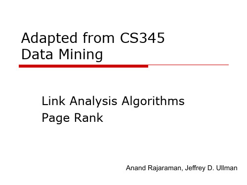
Amazon y a = m 1 1 1
M’soft 1.00 0.60 1.40 0.84 0.60 1.56
y 7/15 7/15 1/15 a 7/15 1/15 1/15 m 1/15 7/15 13/15 0.776 0.536 . . . 1.688 7/11 5/11 21/11
I forget to divide by 3
Are all inlinks equal?
Recursive question!
Simple recursive formulation
Each link’s vote is proportional to the importance of its source page If page P with importance x has n outlinks, each link gets x/n votes Page P’s own importance is the sum of the votes on its inlinks
Matrix formulation
Matrix M has one row and one column for each web page Suppose page j has n outlinks
If j i, then Mij=1/n Else Mij=0
M is a column stochastic matrix
y a = m
M’soft
1/3 1/3 1/3 1/3 1/2 1/6 5/12 1/3 1/4 3/8 11/24 . . . 1/6 2/5 2/5 1/5
Random Walk Interpretation
power bi dax编写时的说明语句

一、power bi dax简介Power BI是微软提供的一款数据分析和可视化工具,而DAX(Data Analysis Expressions)是用于Power BI中的数据分析表达式语言。
在Power BI中使用DAX语言可以进行不同类型的数据计算、过滤和汇总,帮助用户更好地理解数据,做出更准确的决策。
二、DAX语句的排列顺序在编写Power BI的DAX语句时,需要注意语句的排列顺序,以确保语法正确和逻辑清晰。
一般来说,DAX语句可以按照以下顺序排列:1. 声明变量:可以使用VAR关键字声明变量,以便在后续的计算中复用某个表达式的结果。
2. 计算列:可以使用CALCULATE关键字创建计算列,将某个表达式的计算结果作为新的列添加到数据表中。
3. 定义度量值:可以使用DEFINE MEASURE关键字定义度量值,用于在报表中进行汇总和计算。
三、DAX语句的基本语法在编写DAX语句时,需要掌握其基本语法,包括以下几个方面:1. 表达式:DAX语句中的表达式可以是数学运算、逻辑运算、文本操作等,需要根据实际需求选择合适的表达式。
2. 函数:DAX语句中包含了丰富的函数库,用于完成各种数据分析和计算操作,包括聚合函数、数学函数、逻辑函数等。
3. 运算符:DAX语句中包含了各种运算符,包括加减乘除、逻辑运算、文本连接等,需要根据实际需求选择合适的运算符。
四、DAX语句的常见问题及解决方法在编写DAX语句时,可能会遇到一些常见问题,比如语法错误、逻辑错误等,需要注意以下几个方面:1.语法错误:在编写DAX语句时,需要严格按照语法规则进行排列和书写,以避免出现语法错误,需要仔细检查语句的拼写和格式。
2.逻辑错误:在编写DAX语句时,需要确保逻辑的正确性,比如条件判断、数据筛选等,需要对逻辑进行仔细思考和验证。
3.优化性能:在编写DAX语句时,需要考虑计算性能的优化,比如减少不必要的计算、合理使用缓存等,以提高查询和计算的效率。
计算机专业英语第二版 译文

《计算机英语》参考译文(精读部分)目录第1单元课文A:计算机概览 (3)一、引言 (3)二、历史 (3)三、硬件 (4)四、编程 (5)五、未来的发展 (5)第2单元课文A:计算机硬件 (5)一、引言 (5)二、输入硬件 (6)三、输出硬件 (6)四、存储硬件 (7)五、硬件的连接 (7)第3单元课文A:操作系统 (8)一、引言 (8)二、操作系统是怎样工作的 (8)三、当前的操作系统 (8)五、未来的技术 (10)第4单元课文A:编程语言 (11)一、引言 (11)二、语言类型 (11)三、高级语言的分类 (12)四、语言的结构与成分 (12)五、历史 (13)第5单元课文A:计算机程序 (13)一、引言 (13)二、程序开发 (14)三、程序元素 (14)四、程序功能 (15)五、历史 (16)六、未来 (16)第6单元课文A:软件生命周期 (17)第7单元课文A:进入关系数据库的世界 (19)一、什么是关系数据库? (19)二、数据库管理系统的介绍 (20)三、不同的计算模型 (21)第8单元课文A:电信与计算机 (22)第9单元课文A:计算机网络 (24)一、引言 (24)二、调制解调器与计算机管理局 (24)三、局域网 (24)四、路由器与桥接器 (25)五、广域网 (25)六、分布式计算 (25)七、安全与管理 (26)第10单元课文A:因特网是如何工作的? (26)一、因特网访问 (27)二、信息打包 (27)三、网络编址 (27)四、电子邮件 (28)五、传输模式 (28)六、带宽 (28)第11单元课文A:信息革命 (29)一、引言 (29)二、社会与技术发展 (29)三、信息革命的方向 (29)四、就业趋势 (30)五、信息技术与消费者 (31)六、信息革命的问题 (31)第12单元课文A:电子商务简介 (32)一、定义 (32)二、需求与服务 (32)第13单元课文A:计算机安全 (34)一、计算机安全面临的威胁 (34)二、保护计算机安全的措施 (36)第14单元课文A:比尔•盖茨文摘 (37)第1单元课文A:计算机概览一、引言计算机是一种电子设备,它能接收一套指令或一个程序,然后通过对数值数据进行运算或者对其他形式的信息进行处理来执行该程序。
theory-questions
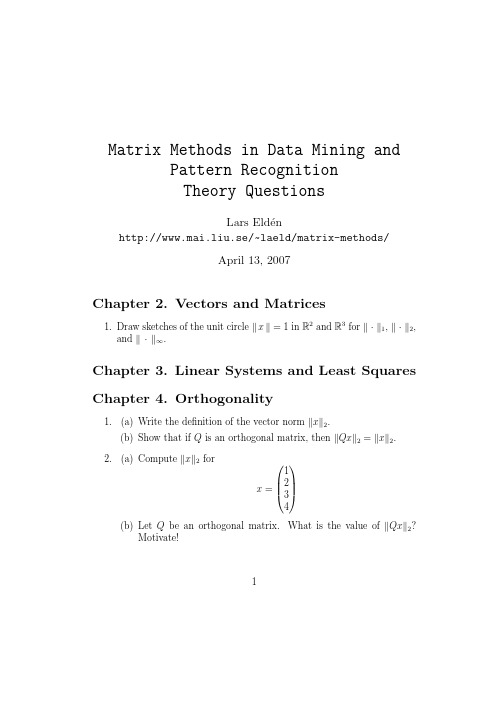
where × denotes non-zero elements. We want to zero the bottom non-zero element in the first column, which assumed to be in row i. Explain why the following code is unsuitable, even if it is correct. G = eye(n); G(i-1:i,i-1:i)=G0; A = G * A; % G0 is a 2 x 2 rotation
Write a better code that does the job. 5. (a) Let P = I − 2uuT be a Householder transformation, and define 1 x = 2 . 3 Compute P x 2 . Motivate the answer. (b) With a Householder matrix one can transform the vector x to a unit vector, P x = κe1 . What is the value of κ?
3. (a) Let the matrices bT 1 bT 2 B=. , . . bT n
A = (a1 a2 . . . an ),
be given, where ai are column vectors and bT i are row vectors. Write the matrix product AB as a sum of rank one matrices. (b) Let A be a matrix of dimension m × n, where m ≥ n, with SVD A=U Σ V T. 0
面向大数据高通量计算的CPU-GPU并行优化技术研究
面向大数据高通量计算的CPU-GPU并行优化技术研究摘要:本文对面向大数据高通量计算的CPU/GPU并行优化技术进行了深入研究。
首先,分析了CPU/GPU并行计算的优势以及不足之处,并探讨了如何合理利用CPU/GPU资源进行高效的并行计算。
其次,本文介绍了大数据高通量计算中常用的算法,包括分布式排序、K-means聚类、PageRank算法等,分析了这些算法在CPU/GPU并行计算中的应用。
然后,作者提出了一套针对大数据高通量计算的CPU/GPU并行优化技术框架,其中包括数据的预处理、算法的并行化、GPU和CPU的协同工作等多个方面的优化措施。
最后,本文采用真实的大数据集进行实验验证,结果表明所提出的优化技术方案具有良好的实用性和优化效果。
关键词:大数据,高通量计算,CPU/GPU并行计算,算法优化,实验验证Abstract:This paper deeply explores the optimization techniques of CPU/GPU parallel computing for large-scale data and high-throughput computing. Firstly, the advantages and disadvantages of CPU/GPU parallel computing are analyzed, and the rational utilization of CPU/GPUresources for efficient parallel computing is discussed. Secondly, this paper introduces the commonly used algorithms in large-scale data and high-throughput computing, including distributed sorting,K-means clustering, PageRank, and analyzes their applications in CPU/GPU parallel computing. Then, the author proposes a framework of CPU/GPU parallel optimization techniques for large-scale data and high-throughput computing, which includes several optimization measures in data preprocessing, algorithm parallelization, and the coordination between GPU and CPU. Finally, the proposed optimization techniques are verified with real-world datasets, and the experimental results show a good practicality and optimization efficiency of the proposed techniques.Keywords: Large-scale data, high-throughput computing, CPU/GPU parallel computing, algorithm optimization, experimental validationIn recent years, with the proliferation of various applications generating massive amounts of data, handling large-scale datasets has become a challenge for many organizations. High-throughput computing, which is a type of computing that emphasizes achieving large amounts of computational work in a scalable and efficient manner, has gained increasing attention as apromising solution to this challenge.To optimize the performance of high-throughput computing in handling large-scale data, several measures have been proposed. One key area is data preprocessing, which aims to reduce the size of the dataset and remove redundant or irrelevant information while retaining the necessary information for analysis. This can involve techniques such as data compression, feature selection, and normalization, and can significantly improve the efficiency of subsequent analysis.Another important area of optimization is algorithm parallelization, which involves dividing the computational workload into multiple concurrent processes or threads that can be executed in parallel. This can be achieved through techniques such asparallel programming, distributed computing, and GPU acceleration. Parallelization can help to reduce the processing time of complex algorithms and enable the analysis of larger datasets.Moreover, to optimize the coordination between CPU and GPU, the use of appropriate APIs and libraries can greatly improve the performance of high-throughput computing. For instance, CUDA is a parallel computingplatform and programming model that enables developers to leverage the power of GPUs, while OpenCL is an open-standard API that enables the development of heterogeneous parallel applications that can run on a variety of hardware platforms.Finally, the proposed optimization techniques in high-throughput computing for handling large-scale data have been validated through experiments with real-world datasets. The experimental results have shown that these techniques can effectively improve the performance and efficiency of high-throughput computing for handling large-scale data, demonstrating their practicality and potential for use in various applicationsIn addition to the techniques mentioned above, there are several emerging trends in high-throughput computing that have the potential to significantly impact how large-scale data is processed and analyzed.One such trend is the use of machine learning and artificial intelligence algorithms to optimize high-throughput computing workflows. By analyzing data patterns and deriving insights from historical performance data, these algorithms can automatically optimize various aspects of the high-throughputcomputing pipeline, including job scheduling, workload balancing, and resource allocation.Another trend is the move towards cloud-based high-throughput computing, where large-scale data analysis is performed on virtual machines running on remote servers. Cloud-based high-throughput computing offers several advantages over traditional on-premises solutions, including scalability, elasticity, andcost-effectiveness.Furthermore, high-throughput computing is increasingly being used in scientific research, especially in areas such as genomics, proteomics, and drug discovery.High-throughput computing is enabling scientists to process and analyze vast amounts of data, leading to new discoveries and insights into complex biological systems.Overall, high-throughput computing is a critical technology for the processing and analysis of large-scale data. With the ever-increasing volume and complexity of data being generated, the optimization techniques and emerging trends discussed in this article will become increasingly important in addressing the challenges of high-throughput computingOne emerging trend in high-throughput computing is the use of cloud computing platforms. These platforms provide scalable and cost-effective computing resources that can be accessed on-demand. This allows researchers to process and analyze large amounts of data without the need for expensive hardware and software investments. Cloud computing also enables collaboration between researchers and institutions, as data and analysis can be easily shared and accessed from multiple locations.Another emerging trend is the use of machine learning algorithms in high-throughput computing. Machine learning algorithms can be trained to identify patterns and relationships in complex datasets, and can be used for tasks such as data classification and prediction. This can significantly speed up the analysis process and allow researchers to extract meaningful insights from large amounts of data.In addition to these trends, there are also ongoing efforts to improve the efficiency and speed of high-throughput computing. This includes the development of new hardware and software technologies, such as faster processing chips and optimized algorithms, as well as the use of parallel processing and distributed computing techniques.Despite these advances, there are still challenges to be addressed in high-throughput computing. One major challenge is the need to ensure data accuracy and reliability, as errors in large datasets can have significant consequences. Another challenge is the need to integrate data from multiple sources, which requires standardized formats and protocols.Overall, high-throughput computing has the potential to revolutionize the fields of biology, medicine, and beyond, enabling researchers to rapidly process and analyze vast amounts of data and uncover new insights into complex biological systems. As the volume and complexity of data continue to increase, it will be important to continue developing new technologies and techniques to address the challenges of high-throughput computing and unlock its full potentialIn conclusion, high-throughput computing has emerged as a powerful tool for processing and analyzing large volumes of data in the fields of biology and medicine. The use of high-throughput technologies, such as NGS and microarrays, has enabled researchers to generate massive amounts of data and gain new insights into complex biological systems. However, with the increasing volume and complexity of data, it iscrucial to continue developing new methods and protocols to address the challenges of high-throughput computing and fully realize its potential. Overall, high-throughput computing has the potential to transform our understanding of biology and medicine and play a vital role in advancing scientific research and discovery。
计算机专业英语

计算机专业英语专业英语习题_7c解释⼀下为啥之前的删了呢?我刚刚考研结束,发现⾃⼰没啥⼈关注,也没啥浏览量,就以为没⼈看,觉得⾃⼰⼜隔这⾃⾔⾃语呢,本着随缘佛系的⼼态就删了;直到很多⼈私信我,我才知道原来是有⼈需要的呀,感谢⼤家的信任!再解释⼀下,题⽬来源问题,部分来⾃课后习题,部分来⾃本校⾬课堂,都是⾃⼰⼀句⼀句从上⾯⽂字识别下来的;⾄于翻译呢,是⾃⼰⼀句⼀句百度啊有道啊啥的⽹站翻译的;答案准确度问题,⾬课堂习题的答案是由⽼师发布的标准答案答案,课后习题答案是⾃⼰从⽹上各种搜索以及结合⾃⼰对课本的理解与把握填上去的,是真的费事,但值得。
有问题随时交流哦,另外也整理了仅含的课后习题版本也发步了哦,新调了下格式⽅便⼤家复习使⽤。
第1章信息技术、互联⽹和你⾬课堂Chapter 01 Lesson testWhich part is the most important of an information system? 信息系统的哪个部分是最重要的? People √ ⼈Which part of an information system consists of the rules or guidelines for people to follow? 信息系统的哪⼀部分包含了⼈们要遵循的规则或指导⽅针? Procedures √ 程序Which part is the second most important of an information system? 哪个部分是信息系统的第⼆重要部分? Data √ 数据[Software] is another name for a program or programs.The Purpose of software is to convert [data](unprocessed facts)into[information](processed facts)软件是程序或程序的另⼀个名称项⽬。
大数据经典算法PageRank 讲解

通过迭代计算每个网页的 PageRank值。
设定阈值,当计算结果变化小于 阈值时停止迭代。
结果
结果展示
以可视化方式展示每个网页的PageRank值 。
结果分析
对结果进行深入分析,挖掘有价值的信息。
结果应用
将PageRank值应用于实际场景,如网页排 名、信息筛选等。
04
CATALOGUE
PageRank算法优化
社交网络的兴起
随着社交媒体的兴起,网页之间的链接关系变得更加复杂 和多样化,需要更复杂的算法来准确计算PageRank值。
算法的可解释性问题
缺乏可解释性
PageRank算法是一个黑箱模型,其运算过程和结果难以 解释,使得人们难以理解其工作原理和决策依据。
可解释性与准确性的权衡
为了提高算法的可解释性,可能会牺牲一定的准确性,这 需要在可解释性和准确性之间进行权衡。
推荐系统
PageRank可以用于推荐系 统,通过分析用户行为和物 品之间的关系,为用户推荐 相关内容。
信息提取和筛选
PageRank可以用于信息提 取和筛选,通过分析网页之 间的链接关系,提取有用的 信息并筛选出高质量的内容 。
02
CATALOGUE
PageRank算法原理
网页链接关系
网页之间的链接关系
链接分析
PageRank算法通过分析网页之间的链接数量和质量,判 断每个网页的价值。一个网页如果有较多的外部链接,且 这些链接都来自质量较高的网页,那么这个网页的 PageRank值就会相应提高。
广告定位
Google AdWords等广告平台也利用PageRank算法,将 广告投放到与内容相关的网页上,从而提高广告的点击率 和转化率。
PageRank外推插值法
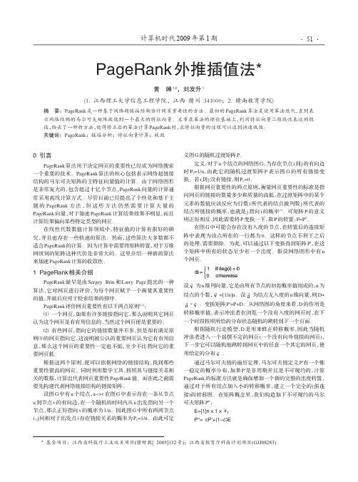
结点的个数, =[1/n]n。设
*
转移概率值, 表示冲浪者在浏览一个没有入度的网页时, 在下 一个时段按照所给的分布状态随机的跳转到下一个页面。 根据随机行走模型, D 是用来修正转移概率, 因此当随机 冲浪者进入一个摇摆不定的网页(一个没有向外链接的网页), 下一步它可以随机地跳转到网页中的任意一个其它的网页, 使 用给定的分布 。 通过马尔可夫链的遍历定理, 马尔可夫链定义 P'有一个惟 一稳定的概率分布, 如果 P'是非周期并且是不可规约的, 计算 PageRank 的标准方法就是确保增加一个新的完整的出度转置, 通过对于所有结点加入小的转移概率, 建立一个完全的(强连 接)的转移图。在矩阵概念里, 我们构造如下不可规约的马尔 可夫矩阵 P'': E=[1]n×1× P''= cP'+(1-c)E
能够用 A 的特征向量 ⑵
由于马尔可夫矩阵的最大特征值λ1=1,
且有 由于λ n≤…≤λ 2<1, 该式右端近似等于 它收敛于马尔可夫矩阵 A 的主特征向量。 影响幂法收敛速度的因素很多, 适当选取起始的
⑷ , 因此当 n 很大时, 可以
组合表示的假定, 等式⒂只是给出了向量 出了外推插值法与幂法相结合估算
参考文献:
[1] L. Page, S. Brin, R. Motwani, and T. Winograd. The PageRank citation ranking: Bringing order to the web[J].Stanford Digital Libraries Working Paper,1998. [2] T. H. Haveliwala, topic-sensitive PageRank[C]. In Proceedings of the Eleventh International World Wide Web Conference,2002. [3] G. Jeh and J. Widom. Scaling personalized web search[C]. In Proceedings of the Twelfth International World Wide Web Conference,2003. [4] Soumen Chakrabarti, Martin van den Berg, Byron Dom, Focused crawling:a new approach To topic-specific Web-Experiments and algorithms[J],2002. [5] 张延红. 搜索引擎 PageRank 算法的改进[J]. 浙江万里学院学报, 2005.18(4). [6] T H Haveliwala, S D Kamvar, Dan Klein et puting PageRank using Power Extrapolation[R]. Technical Report, Standford University,2003.
power query m语言 应用实例

Power Query M语言是一种用于数据处理和转换的强大工具,它可以帮助用户轻松地从各种数据源中提取、转换和加载数据。
在本文中,我们将介绍Power Query M语言的应用实例,通过具体的案例来展示其在数据处理中的强大功能和灵活性。
1. 数据提取在实际的数据处理过程中,我们经常需要从各种数据源中提取数据。
Power Query M语言可以帮助我们轻松地实现这一目标。
我们可以使用Power Query M语言编写一段代码,从Excel表格中提取特定的数据,并将其加载到Power BI中进行分析和可视化。
2. 数据转换除了数据提取,数据转换也是数据处理过程中不可或缺的一部分。
Power Query M语言提供了丰富的数据转换函数,可以帮助我们对数据进行各种复杂的转换操作。
我们可以使用Power Query M语言编写一段代码,将某个日期字段转换为季度字段,从而方便我们对数据进行更深入的分析。
3. 数据加载一旦数据提取和转换完成,我们就需要将数据加载到目标系统中进行进一步的处理和分析。
Power Query M语言可以帮助我们将数据加载到各种目标系统中,如SQL数据库、Excel表格等。
我们可以使用Power Query M语言编写一段代码,将数据加载到SQL数据库中,并创建相应的数据表,以便后续的数据处理和分析。
通过上述实例,我们不难看出,Power Query M语言在数据处理中具有非常强大的功能和灵活性。
它可以帮助我们轻松地实现数据提取、转换和加载等操作,提高数据处理的效率和准确性,为我们的工作和决策提供更加可靠的数据支持。
掌握Power Query M语言的应用技巧,对于数据分析师和数据处理人员来说是非常重要的。
希望本文的介绍能够帮助读者更好地理解和应用Power Query M语言,从而更加高效地处理和分析数据。
4. 数据合并在实际的数据处理中,我们经常需要将来自不同数据源的数据进行合并。
pagerank算法讲解

Google的网页排序
如何度量网页本身的重要性呢?
比如,新华网体育在其首页中对新浪体育做了链接, 人民网体育同样在其首页中对新浪体育做了链接
新华网体育
人民网体育
可见,新浪体育被链接的次数较多;同时,人民网体 育和新华网体育也都是比较“重要”的网页,因此新 浪体育也应该是比较“重要”的网页。
① 这种随机模型更加接近于用户的浏览行为; ② 一定程度上解决了rank leak和rank sink的问题; ③ 保证pagerank具有唯一值。
随机浏览模型的图表示
设定任意两个顶点之间都有直接通路, 在每个顶点处以概率d按原来蓝色方向转移,以概率1d按红色方向转移。
随机浏览模型的邻接表表示
由于网页数目巨大,网页之间的连接关系的邻接矩阵是一个很 大的稀疏矩阵,采用邻接表来表示网页之间的连接关系.随机浏览模 型的PageRank公式:
目录
背景介绍 Google的网页排序 PageRank简化模型 PageRank随机浏览模型 PageRank的计算
Google的网页排序
在Google中搜索“体育新闻”
Google的网页排序
查询词和文档的相关性
在Google中搜索“体育新闻”
搜索引擎工作的简要过程如下
针对查询词“体育新闻”进行分词——》“体育”、“新 闻”
换句话说,根据链出总数平分一个页面的PR值。
PageRank的简单计算过程
PRi
jBi
PRj Lj
PageRank的简化模型
可以把互联网上的各网页之间的链接关系看成一个有向 图。假设冲浪者浏览的下一个网页链接来自于当前网页。 建立简化模型:对于任意网页Pi,它的PageRank值可表 示为如下:其中Bi为所有链接到网页i的网页集合,Lj为 网页j的对外链接数(出度)。
PageRank的快速计算

PageRank的快速计算
在互联网中寻找网页重要性(PR值)及排序,需要用到迭代进行矩阵-向量乘法计算,其中由于需要处理的数据规模极大,矩阵和向量的维度达到几百亿维,而我们又需要快速计算处理,因此在数据挖掘过程中MapReduce方法的实现原理和机制值得推荐。
MapReduce方法可以被看成一种对数据的高效梳理方法,以避免杂乱而不好提取其信息价值。
类似于我们手头有一堆发票,如果只管不理,还是价值一般的一堆发票。
如何实现既“管”又“理”呢?当然需要对数据特征进行识别、提取和恰当的记录,如把发票中的时间、金额、开票项目、单号和抬头等一系列特征信息抽取出来,制成Excel 表格,就可以更高效地进行快速梳理。
而MapReduce的本质也是把一堆杂乱无章的数据按照某种特征归纳起来,然后处理并得到最后的结果。
MapReduce面对的是杂乱无章的、互不相关的数据,它解析每个数据,从中提取出key和value(k,v)值,也就是提取了数据的特征。
经过MapReduce的Shuffle洗牌阶段之后,在Reduce阶段看到的都是已经归纳好的数据,在此基础上我们可以做进一步的处理以便得到相应的结果。
MapReduce工作流程如图1所示。
由于互联网上的转移矩阵M非常稀疏,如果矩阵中所有元素都参与计算,则效率很低,所以我们可以对矩阵做进一步压缩处理。
同时,迭代计算资源反复调用开销过大,会导致系统产生内存抖动。
因此在计算PR值时,我们考虑只有非零元素参与计算,或者减少Map任务必须传给Reduce任务的数据量,以实现PageRank的快速计算。
power bi 复杂函数
Power BI 提供了许多复杂的函数,用于帮助用户在数据分析和可视化方面进行更高级的操作。
以下是一些Power BI 的复杂函数示例:1. DAX 函数:DAX(Data Analysis Expressions)是Power BI 使用的公式语言,用于进行复杂的数据分析和计算。
DAX 函数可以用于创建计算列、计算汇总值、筛选数据等等。
例如,以下DAX 函数可以计算销售数据的总额:`Total Sales = SUM('Sales'[Amount])`2. SQL 函数:Power BI 还可以使用SQL 函数来处理数据。
例如,可以使用SQL 的`LEFT()`、`RIGHT()`、`SUBSTRING()` 等函数来对文本数据进行处理,使用`DATEADD()` 函数来对日期数据进行处理。
3. M语言函数:M 语言是Power BI Desktop 使用的语言,可以用于编写自定义函数、调试公式等。
M 语言函数可以使用Power BI 的API 和功能来扩展Power BI 的功能。
4. R语言函数:Power BI R 包可以让你在Power BI 中使用R 语言函数。
R 语言是一种广泛使用的统计计算语言,可以用于数据清洗、数据预处理、分析和可视化等方面。
5. Python 函数:Power BI Python 包可以让你在Power BI 中使用Python 语言函数。
Python 是一种广泛使用的编程语言,可以用于数据清洗、数据预处理、分析和可视化等方面。
以上是一些Power BI 的复杂函数示例,希望能够对您有所帮助。
如果您需要更多帮助,请查阅相关文档或咨询专业人士。
power bi ptm计算公式

power bi ptm计算公式Power BI是一种数据可视化和商业智能工具,它可以帮助用户从多个数据源中提取、转换和加载数据,并通过创建交互式报表和仪表板来展示数据。
其中PTM(Power Tools for Power BI)是Power BI的一个插件,它提供了一些额外的功能和计算公式,使用户可以更好地分析和解释数据。
本文将介绍PTM计算公式的使用方法和效果。
一、PTM计算公式的概述PTM计算公式是Power BI中的一种功能,它可以通过使用特定的语法和函数来对数据进行计算和转换。
使用PTM计算公式可以轻松实现数据的聚合、过滤、排序、计数等操作,以及创建自定义的度量和指标。
下面我们将介绍几个常用的PTM计算公式。
二、SUMM函数SUMM函数是PTM中用于求和的函数,它可以对一个列或表达式中的数值进行求和操作。
例如,我们可以使用SUMM函数计算销售额的总和或某个时间段内的销售额总和。
三、AVER函数AVER函数是PTM中用于求平均值的函数,它可以对一个列或表达式中的数值进行平均值计算。
例如,我们可以使用AVER函数计算某个地区的平均销售额或某个时间段内的平均销售额。
四、COUNTM函数COUNTM函数是PTM中用于计数的函数,它可以统计一个列或表达式中的非空值的个数。
例如,我们可以使用COUNTM函数统计销售额不为零的订单数量或某个时间段内的订单数量。
五、FILTER函数FILTER函数是PTM中用于过滤数据的函数,它可以根据指定的条件对数据进行筛选。
例如,我们可以使用FILTER函数筛选出销售额大于1000的订单或某个时间段内的订单。
六、RANKX函数RANKX函数是PTM中用于排序数据的函数,它可以根据指定的列或表达式对数据进行排序。
例如,我们可以使用RANKX函数对销售额进行排序,从而找出销售额排名前五的产品或某个时间段内销售额排名前五的产品。
七、总结通过使用PTM计算公式,我们可以更加灵活地对数据进行分析和计算。
USM博士研究计划书

USM博士研究计划书1. 研究背景USM(Ultra-Scale Computing and Systems)是一项旨在实现超级计算和系统的研究项目。
随着科学技术的不断发展,对于高性能计算和系统需求的增加,传统计算机体系结构已经无法满足如此巨大规模的数据处理要求。
因此,USM计划旨在通过研究新的计算机架构和系统,为超级计算机的发展提供技术支持和创新。
2. 研究目标本研究计划的目标是设计和开发一种高效的超级计算机架构和系统,以应对日益增长的计算和存储需求。
具体而言,我们的目标是:•提高计算机系统的处理性能,将其提升到新的高度;•加强计算机系统的扩展性,使其能够支持更大规模的并行计算;•降低能耗,提高计算机系统的性能功耗比;•设计和开发适用于特定应用场景的优化算法和编程模型。
3. 研究内容本研究计划主要包括以下几个方面的内容:3.1 超级计算机架构设计•分析和评估现有超级计算机架构的优缺点;•设计一种新的计算机架构,具有更好的性能和可扩展性;•研究新的内存层次结构和存储系统,以提高计算机系统的存储和访问效率。
3.2 超级计算机系统开发•开发适用于超级计算机架构的操作系统和运行时环境;•研究和实现高性能和高可用性的通信和数据传输机制;•设计和开发系统监控和调优工具,以改善计算机系统的性能和效率。
3.3 算法和编程模型优化•研究现有算法和编程模型在超级计算机上的性能表现;•提出针对特定计算机架构优化的算法和编程模型;•开发高效的并行编程工具和库,以支持复杂的科学计算和数据分析。
4. 研究计划4.1 第一阶段:调研和需求分析(计划时间:3个月)•调研现有超级计算机架构和系统的最新研究成果;•分析和评估现有超级计算机的性能和可扩展性;•收集并分析用户的需求和使用场景。
4.2 第二阶段:架构设计和系统开发(计划时间:12个月)•设计新的超级计算机架构,并进行模拟和评估;•开发适用于新架构的操作系统和运行时环境;•实现高性能通信和数据传输机制;•设计和开发系统监控和调优工具。
dax练习题

DAX练习题一、基础概念题1. 请简述DAX是什么以及其主要功能。
2. 解释DAX中的度量值与计算列的区别。
3. 请列举DAX中常用的几种数据类型。
4. 描述DAX中的筛选上下文和行上下文的概念。
5. 请说明如何在DAX中使用时间智能函数。
二、数据操作题1. 使用DAX创建一个计算列,计算每个订单的利润。
2. 使用DAX创建一个度量值,计算总销售额。
3. 使用DAX创建一个度量值,计算平均订单金额。
4. 使用DAX创建一个度量值,计算当前年份的累计销售额。
5. 使用DAX创建一个度量值,计算各产品类别的销售额占比。
6. 使用DAX创建一个度量值,计算各月份的销售额增长率。
三、数据筛选题1. 使用DAX筛选出销售额大于10000的订单。
2. 使用DAX筛选出订单日期在2021年的订单。
3. 使用DAX筛选出销售额排名前10%的订单。
4. 使用DAX筛选出各产品类别中销售额最高的订单。
5. 使用DAX筛选出各月份销售额最高的订单。
四、数据聚合题1. 使用DAX计算各产品类别的总销售额。
2. 使用DAX计算各年份的总销售额。
3. 使用DAX计算各月份的总销售额。
4. 使用DAX计算各省份的总销售额。
5. 使用DAX计算各销售员的总销售额。
五、数据转换题1. 使用DAX将日期列转换为年份和月份。
2. 使用DAX将销售额列转换为销售额等级(如:低、中、高)。
3. 使用DAX将产品名称列转换为产品类别。
4. 使用DAX将订单状态列转换为订单状态颜色(如:绿色、红色、黄色)。
5. 使用DAX将销售员姓名列转换为销售员级别(如:初级、中级、高级)。
六、数据计算题1. 使用DAX计算各产品类别的平均销售额。
2. 使用DAX计算各年份的平均销售额。
3. 使用DAX计算各月份的平均销售额。
4. 使用DAX计算各省份的平均销售额。
5. 使用DAX计算各销售员的平均销售额。
七、数据排序题1. 使用DAX按照销售额降序排列订单。
- 1、下载文档前请自行甄别文档内容的完整性,平台不提供额外的编辑、内容补充、找答案等附加服务。
- 2、"仅部分预览"的文档,不可在线预览部分如存在完整性等问题,可反馈申请退款(可完整预览的文档不适用该条件!)。
- 3、如文档侵犯您的权益,请联系客服反馈,我们会尽快为您处理(人工客服工作时间:9:00-18:30)。
Computing PageRank using Power ExtrapolationTaher Haveliwala,Sepandar Kamvar,Dan Klein,Chris Manning,and Gene GolubStanford UniversityAbstract.We present a novel technique for speeding up the computation ofPageRank,a hyperlink-based estimate of the“importance”of Web pages,basedon the ideas presented in[7].The original PageRank algorithm uses the PowerMethod to compute successive iterates that converge to the principal eigenvec-tor of the Markov matrix representing the Web link graph.The algorithm pre-sented here,called Power Extrapolation,accelerates the convergence of the PowerMethod by subtracting off the error along several nonprincipal eigenvectors fromthe current iterate of the Power Method,making use of known nonprincipal eigen-values of the Web hyperlink matrix.Empirically,we show that using Power Ex-trapolation speeds up PageRank computation by30%on a Web graph of80mil-lion nodes in realistic scenarios over the standard power method,in a way that issimple to understand and implement.1IntroductionThe PageRank algorithm for determining the“importance”of Web pages has become a central technique in Web search[9].The core of the PageRank algorithm involves computing the principal eigenvector of the Markov matrix representing the hyperlink structure of the Web.As the Web graph is very large,containing over a billion nodes, the PageRank vector is generally computed offline,during the preprocessing of the Web crawl,before any queries have been issued.The development of techniques for computing PageRank efficiently for Web-scale graphs is important for a number of reasons.For Web graphs containing a billion nodes, computing a PageRank vector can take several puting PageRank quickly is necessary to reduce the lag time from when a new crawl is completed to when that crawl can be made available for searching.Furthermore,recent approaches to person-alized and topic-sensitive PageRank schemes[2,10,6]require computing many Page-Rank vectors,each biased towards certain types of pages.These approaches intensify the need for faster methods for computing PageRank.A practical extrapolation method for accelerating the computation of PageRank was first presented by Kamvar et al.in[7].That work assumed that none of the nonprinci-pal eigenvalues of the hyperlink matrix were known.Haveliwala and Kavmar derived the modulus of the second eigenvalue of the hyperlink matrix in[3].By exploiting known eigenvalues of the hyperlink matrix,we derive here a simpler and more effec-tive extrapolation algorithm.We show empirically on an80million page Web crawl that this algorithm speeds up the computation of PageRank by30%over the standard power method.The speedup in number of iterations is basically equivalent to that of the Quadratic Extrapolation algorithm introduced in[7],but the method presented here ismuch simpler to implement,and has negligible overhead,so that its wallclock-speedup is higher by9%.12PreliminariesIn this section we summarize the definition of PageRank[9]and review some of the mathematical tools we will use in analyzing and improving the standard iterative algo-rithm for computing PageRank.Underlying the definition of PageRank is the following basic assumption.A link from a page u∈Web to a page v∈Web can be viewed as evidence that v is an “important”page.In particular,the amount of importance conferred on v by u is pro-portional to the importance of u and inversely proportional to the number of pages u points to.Since the importance of u is itself not known,determining the importance for every page i∈Web requires an iterativefixed-point computation.To allow for a more rigorous analysis of the necessary computation,we next de-scribe an equivalent formulation in terms of a random walk on the directed Web graph G.Let u→v denote the existence of an edge from u to v in G.Let deg(u)be the out-degree of page u in G.Consider a random surfer visiting page u at time k.In the next time step,the surfer chooses a node v i from among u’s out-neighbors{v|u→v}uni-formly at random.In other words,at time k+1,the surfer lands at node v i∈{v|u→v} with probability1/deg(u).The PageRank of a page i is defined as the probability that at some particular time step k>K,the surfer is at page i.For sufficiently large K,and with minor modifi-cations to the random walk,this probability is unique,illustrated as follows.Consider the Markov chain induced by the random walk on G,where the states are given by the nodes in G,and the stochastic transition matrix describing the transition from i to j is given by P with P ij=1/deg(i).For P to be a valid transition probability matrix,every node must have at least1 outgoing transition;i.e.,P should have no rows consisting of all zeros.This holds if G does not have any pages with outdegree0,which does not hold for the Web graph. P can be converted into a valid transition matrix by adding a complete set of outgoing transitions to pages with outdegree0.In other words,we can define the new matrix P where all states have at least one outgoing transition in the following way.Let n be the number of nodes(pages)in the Web graph.Let v be the n-dimensional column vector representing a uniform probability distribution over all nodes:1v=[1Note that as the Quadratic Extrapolation algorithm of[7]does not assume the second eigen-value of the matrix is known,it is more widely applicable(but less efficient)than the algo-rithms presented here.y=cP T x;w=||x||1−||y||1;y=y+w v;Algorithm1:Computing y=A xThen we construct P as follows:D=d·v TP =P+DIn terms of the random walk,the effect of D is to modify the transition probabilities so that a surfer visiting a dangling page(i.e.,a page with no outlinks)randomly jumps to another page in the next time step,using the distribution given by v.By the Ergodic Theorem for Markov chains[1],the Markov chain defined by P has a unique stationary probability distribution if P is aperiodic and irreducible;the former holds for the Markov chain induced by the Web graph.The latter holds iff G is strongly connected,which is generally not the case for the Web graph.In the context of computing PageRank,the standard way of ensuring this property is to add a new set of complete outgoing transitions,with small transition probabilities,to all nodes, creating a complete(and thus strongly connected)transition graph.In matrix notation, we construct the irreducible Markov matrix P as follows:E=[1]n×1×v TP =cP +(1−c)EIn terms of the random walk,the effect of E is as follows.At each time step,with probability(1−c),a surfer visiting any node will jump to a random Web page(rather than following an outlink).The destination of the random jump is chosen according to the probability distribution given in v.Artificial jumps taken because of E are referred to as teleportation.By redefining the vector v given in Equation1to be nonuniform,so that D and E add artificial transitions with nonuniform probabilities,the resultant PageRank vector can be biased to prefer certain kinds of pages.For this reason,we refer to v as the personalization vector.For simplicity and consistency with prior work,the remainder of the discussion will be in terms of the transpose matrix,A=(P )T;i.e.,the transition probability distribution for a surfer at node i is given by row i of P ,and column i of A.Note that the edges artificially introduced by D and E never need to be explicitly materialized,so this construction has no impact on efficiency or the sparsity of the matrices used in the computations.In particular,the matrix-vector multiplication y= A x can be implemented efficiently using Algorithm1.Assuming that the probability distribution over the surfer’s location at time0is given by x(0),the probability distribution for the surfer’s location at time k is given by x(k)=A k x(0).The unique stationary distribution of the Markov chain is defined aslim k→∞x(k),which is equivalent to lim k→∞A k x(0),and is independent of the initial distribution x(0).This is simply the principal eigenvector of the matrix A=(P )T, which is exactly the PageRank vector we would like to compute.The standard PageRank algorithm computes the principal eigenvector by starting with the uniform distribution x(0)=v and computing successive iterates x(k)= A x(k−1)until convergence.This is known as the Power Method,and is discussed in further detail in Section4.We present here a technique,called Power Extrapolation,that accelerates the con-vergence of the Power Method by subtracting off thefirst few nonprincipal eigenvectors from the current iterate x(k).We take advantage of the fact that thefirst eigenvalue of A is1(because A is stochastic),and the modulus of the second eigenvalues is c(see[3]), to compute estimates of the error along nonprincipal eigenvectors using two iterates of the Power Method.This Power Extrapolation calculation is easy to integrate into the standard PageRank algorithm and yet provides substantial speedups.3Experimental SetupIn the following sections,we will be introducing a series of algorithms for computing PageRank,and discussing the rate of convergence achieved on realistic datasets.Our ex-perimental setup was as follows.We used the L ARGE W EB link graph,generated from a crawl of the Web by the Stanford WebBase project in January2001[4].L ARGE W EB contains roughly80M nodes,with close to a billion links,and requires3.6GB of stor-age.Dangling nodes were removed as described in[9].The graph was stored using an adjacency list representation,with pages represented by4-byte integer identifiers.On an AMD Athlon1533MHz machine with a2-way linear RAID disk volume and3.5GB of main memory,each iteration of Algorithm1on the80M page L ARGE W EB dataset takes roughly10minutes.Given that the full Web contains billions of pages,and com-puting PageRank generally requires roughly50applications of Algorithm1,the need for fast methods is clear.We measured the relative rates of convergence of the algorithms that follow using the L1norm of the residual vector;i.e.,||Ax(k)−x(k)||1See[7]for discussion of measures of convergence for page importance algorithms.4Power Method4.1FormulationOne way to compute the stationary distribution of a Markov chain is by explicitly com-puting the distribution at successive time steps,using x(k)=A x(k−1),until the distri-bution converges.This leads us to Algorithm2,the Power Method for computing the principal eigen-vector of A.The Power Method is the oldest method for computing the principal eigen-vector of a matrix,and is at the heart of both the motivation and implementation of the original PageRank algorithm(in conjunction with Algorithm1).function x(n)=PowerMethod(){x(0)=v;k=1;repeatx(k)=A x(k−1);δ=||x(k)−x(k−1)||1;k=k+1;untilδ< ;}Algorithm2:Power MethodThe intuition behind the convergence of the power method is as follows.For sim-plicity,assume that the start vector x(0)lies in the subspace spanned by the eigenvectors of A.2Then x(0)can be written as a linear combination of the eigenvectors of A:x(0)=u1+α2u2+...+αm u m(2) Since we know that thefirst eigenvalue of a Markov matrix isλ1=1,x(1)=A x(0)=u1+α2λ2u2+...+αmλm u m(3) andx(n)=A n x(0)=u1+α2λn2u2+...+αmλn m u m(4) Sinceλn≤...≤λ2<1,A(n)x(0)approaches u1as n grows large.Therefore,the Power Method converges to the principal eigenvector of the Markov matrix A.4.2Operation CountA single iteration of the Power Method consists of the single matrix-vector multiply A x(k).Generally,this is an O(n2)operation.However,if the matrix-vector multiply is performed as in Algorithm1,the matrix A is so sparse that the matrix-vector multiply is essentially O(n).In particular,the average outdegree of pages on the Web has been found to be around7[8].On our datasets,we observed an average of around8outlinks per page.It should be noted that ifλ2is close to1,then the power method is slow to converge, because n must be large beforeλn2is close to0.4.3Results and DiscussionAs we show in[3],the eigengap1−|λ2|for the Web Markov matrix A is given exactly by the teleport probability1−c.Thus,when the teleport probability is large,the Power Method works reasonably well.However,for a large teleport probability(and with a0.00010.0010.010.1110L 1 r e s i d u a l # of iterations parison of convergence rate for the standard Power Method on the L ARGE W EB dataset for c ∈{0.80,0.85,0.90}.uniform personalization vector v ),the effect of link spam is increased,and pages can achieve unfairly high rankings.3In Figure 1,we show the convergence on the L ARGE W EB dataset of the Power Method for c ∈{0.80,0.85,0.90}using a uniform damping vector v .Note that in-creasing c slows down convergence.Since each iteration of the Power Method takes 10minutes,computing 50iterations requires over 8hours.As the full Web is estimated to contain over two billion static pages,using the Power Method on Web graphs close to the size of the Web would require several days of computation.In the next sections,we describe how to remove the error components of x (k )along the directions of the nonprincipal eigenvectors,thus increasing the effectiveness of Power Method iterations.5Extrapolation MethodsA practical extrapolation method for accelerating the computation of PageRank was first presented by Kamvar et al.in [7].That work assumed that none of the nonprincipal eigenvalues of the hyperlink matrix are known.However,Haveliwala and Kamvar [3]proved that the modulus of the second eigenvalue of A is given by the damping factor c .Note that the web graph can have many eigenvalues with modulus c (i.e.,one of c ,−c ,ci ,and −ci ).In this section,we present a series of algorithms that exploit known eigenvalues of A to accelerate the Power Method for computing PageRank.5.1Simple ExtrapolationFormulation The simplest extrapolation rule assumes that the iterate x(k−1)can be ex-pressed as a linear combination of the eigenvectors u1and u2,where u2has eigenvalue c.x(k−1)=u1+α2u2(5) Now consider the current iterate x(k);because the Power Method generates iterates by successive multiplication by A,we can write x(k)asx(k)=A x(k−1)(6)=A(u1+α2u2)(7)=u1+α2λ2u2(8)Plugging inλ2=c,we see thatx(k)=u1+α2c u2(9)This allows us to solve for u1in closed form:x(k)−c x(k−1)u1=1e-050.00010.0010.010.1110L 1 r e s i d u a l # of iterations parison of convergence rates for Power Method and Simple Extrapolation on L ARGE W EB for c =0.85.Plugging in λ2=c and λ3=−c ,we see thatx (k )=u 1+c 2(α2u 2+α3u 3)(15)This allows us to solve for u 1in closed form:u 1=x (k )−c 2x (k −2)0.00010.0010.010.1110L 1 r e s i d u a l # of iterations parison of convergence rates for Power Method and A 2Extrapolation on L ARGE W EB for c =0.85.We make the assumption that x (k −d )can be expressed as a linear combination of the eigenvectors {u 1...u d +1},where the eigenvalues of {u 2...u d +1}are the d th roots of unity,scaled by c .x (k −d )=u 1+d +1 i =2αi u i (17)Then consider the current iterate x (k );because the Power Method generates iterates by successive multiplication by A ,we can write x (k )asx (k )=A d x (k −d )(18)=A d (u 1+d +1 i =2αi u i )(19)=u 1+d +1 i =2αi λd i u i(20)(21)But since λi is cd i ,where d i is a d th root of unity,x (k )=u 1+c d d +1i =2αi u i (22)(23)This allows us to solve for u 1in closed form:u 1=x (k )−c d x (k −d )function x∗=PowerExtrapolation(x(k−d),x(k)){x∗=(x(k)−c d x(k−d))(1−c d)−1;}Algorithm3:Power Extrapolationfunction x(n)=ExtrapolatedPowerMethod(d){x(0)=v;k=1;repeatx(k)=A x(k−1);δ=||x(k)−x(k−1)||1;if k==d+2,x(k)=P owerExtrapolation(x(k−d),x(k));k=k+1;untilδ< ;}Algorithm4:Power Method with Power Extrapolation For instance,for d=4,the assumption made is that the nonprincipal eigenvalues of modulus c are given by c,−c,ci,and−ci(i.e.,the4th roots unity).A graph in which the leaf nodes in the SCC graph contain only cycles of length l,where l is any divisor of d=4has exactly this property.Algorithms3and4show how to use A d Extrapolation in conjunction with the Power Method.Note that Power Extrapolation with d=1is just Simple Extrapolation. Operation Count The overhead in performing the extrapolation shown in Algorithm3 comes from computing the linear combination(x(k)−c d x(k−d))(1−c d)−1,an O(n) computation.In our experimental setup,the overhead of a single application of Power Extrapo-lation is1%the cost of a standard power iteration.Furthermore,Power Extrapolation needs to be applied only once to achieve the full benefit.Results and Discussion In our experiments,A d Extrapolation performs the best for d=6.Figure4plots the convergence of A d Extrapolation for d∈{1,2,4,6,8},as well as of the standard Power Method,for c=0.85and c=0.90.The wallclock speedups,compared with the standard Power Method,for these5 values of d for c=0.85are given in Table1.For comparison,Figure5compares the convergence of the Quadratic Extrapolated PageRank with A6Extrapolated PageRank.Note that the speedup in convergence is similar;however,A6Extrapolation is much simpler to implement,and has negligi-ble overhead,so that its wallclock-speedup is higher.In particular,each application of Quadratic Extrapolation requires32%of the cost of an iteration,and must be applied several times to achieve maximum benefit.L 1 r e s i d u a l# of iterationsL 1 r e s i d u a l# of iterations(a)c=0.85(b)c=0.90Fig.4.Convergence rates for A d Extrapolation,for d ∈{1,2,4,6,8},compared with standard Power Method.1e-050.0001 0.001 0.01 0.1 1 10L 1 r e s i d u a l# of iterationsparison of convergence rates for Power Method,A 6Extrapolation,and Quadratic Extrapolation on L ARGE W EB for c =0.85.6AcknowledgementsThis paper is based on work supported in part by the National Science Foundation under Grants No.IIS-0085896and CCR-9971010,and in part by the Research Collaboration between NTT Communication Science Laboratories,Nippon Telegraph and Telephone Corporation and CSLI,Stanford University (research project on Concept Bases for Lex-ical Acquisition and Intelligently Reasoning with Meaning).Table1.Wallclock speedups for A d Extrapolation,for d∈1,2,4,6,8,and Quadratic Extrapola-tionType-28%18%25.8%30%21.8%20.8%References1.G.Grimmett and D.Stirzaker.Probability and Random Processes.Oxford University Press,1989.2.T.H.Haveliwala.Topic-sensitive PageRank.In Proceedings of the Eleventh InternationalWorld Wide Web Conference,2002.3.T.H.Haveliwala and S.D.Kamvar.The second eigenvalue of the Google matrix.StanfordUniversity Technical Report,2003.4.J.Hirai,S.Raghavan,H.Garcia-Molina,and A.Paepcke.WebBase:A repository of webpages.In Proceedings of the Ninth International World Wide Web Conference,2000.5. D.L.Isaacson and R.W.Madsen.Markov Chains:Theory and Applications,chapter IV,pages126–127.John Wiley and Sons,Inc.,New York,1976.6.G.Jeh and J.Widom.Scaling personalized web search.In Proceedings of the TwelfthInternational World Wide Web Conference,2003.7.S.D.Kamvar,T.H.Haveliwala,C.D.Manning,and G.H.Golub.Extrapolation methodsfor accelerating PageRank computations.In Proceedings of the Twelfth International World Wide Web Conference,2003.8.J.Kleinberg,S.R.Kumar,P.Raghavan,S.Rajagopalan,and A.Tomkins.The web as agraph:Measurements,models,and methods.In Proceedings of the International Conference on Combinatorics and Computing,1999.9.L.Page,S.Brin,R.Motwani,and T.Winograd.The PageRank citation ranking:Bringingorder to the web.Stanford Digital Libraries Working Paper,1998.10.M.Richardson and P.Domingos.The intelligent surfer:Probabilistic combination of link andcontent information in PageRank.In Advances in Neural Information Processing Systems, volume14.MIT Press,Cambridge,MA,2002.AppendixThis appendix repeats Theorem IV.2.5from[5].Theorem1.(Theorem IV.2.5from[5])If P is the transition matrix of an irreducible periodic Markov chain with period d,then the d th roots of unity are eigenvalues of P. Further,each of these eigenvalues is of multiplicity one and there are no other eigen-values of modulus1.。
