SYSWELD之T型接头建模及网格划分
T型接头模拟

SYSWELD – Welding Wizard
32
1
4
Copyright © ESI Group, 2006. All rights reserved.
5
2 3
6
ESI Group Learning Solutions
SYSWELD – Welding Wizard
33
求解
整个模拟求解自动完成。
SYSWELD – Welding Wizard
11
加载函数库
Copyright © ESI Group, 2006. All rights reserved.
加载工作目录下函数库 文件 hsf.fct
ESI Group Learning Solutions
SYSWELD – Welding Wizard
Copyright © ESI Group, 2006. All rights reserved.
ESI Group Learning Solutions
SYSWELD – Welding Wizard
34
2
ESI Group Learning Solutions
SYSWELD – Welding Wizard
5
载入材料数据库
Copyright © ESI Group, 2006. All rights reserved.
6
加载材料库
Copyright © ESI Group, 2006. All rights reserved.
加载材料库
ESI Group Learning Solutions
SYSWELD – Welding Wizard
7
加载材料库
SYSWELD中文教程T型
(使用软件版本,sysweld2010,pam-assembly2009,weld-planner2009)一、软件安装说明软件包括,sysweld2010,pam-assembly2009,weld-planner2009,其中pam-assembly2009,weld-planner2009统一叫做WeldingDE09,安装基本相同,点击setup,所有选项默认,点击next按钮,直到安装完成,点击finish。
所有安装完毕后,重启计算机,在桌面上出现ESI GROUP 文件夹,所有软件的快捷方式都在此文件夹内。
二、基本流程中小件焊接过程模拟分析的步骤是CAD->网格划分(Visual-mesh)->热源校核(sysweld软件中的Heat Input Fitting)->焊接向导(sysweld软件中的welding wizrad)->求解(sysweld slover)->后处理观察结果(sysweld)网格网格划分是有限元必需的步骤。
Sysweld的网格划分工具采用visual-mesh。
版本使用的是Visual –mesh界面见下图对于形状简单的零件,可以在visual-mesh里面直接建立模型,进行网格划分,对于复杂的图形,需要先在CAD画图软件中画出零件的3维几何图形,然后导入visual-mesh软件进行网格划分。
Visual-mesh的菜单命令中的Curve,Surface,Volume,Node是用来创建几何体的命令,接下来的1D,2D,3D是用来创建1维,2维,3维网格的命令。
对于一个简单的焊接零件,网格创建的步骤为:建立节点nodes生成面surface网格生成a)生成2D mesh 用于生成3D网格b)拉伸3D mesh 用于定义材料赋值及焊接计算c)提取2D mesh表面网格用于定义表面和空气热交换d)生成1D 焊接线,参考线用于描述热源轨迹添加网格组a)开始点,结束点,开始单元用于描述热源轨迹b)装夹点用于定义焊接过程中的装夹条件下面以T型焊缝网格划分为例,说明visual-mesh的具体用法,常用快捷键说明:按住A移动鼠标或者按住鼠标中键,旋转目标;按住S移动鼠标,平移目标;按住D移动鼠标,即为缩放;按F键(Fit),全屏显示;选中目标,按H键(Hide),隐藏目标;选中目标,按L键(Locate),隐藏其他只显示所选并全屏显示;Shift+A,选中显示的全部内容;鼠标可以框选或者点选目标,按住Shift键为反选;在任务进行中,鼠标中键一般为下一步或者确认。
焊接模拟sysweld详细教程
目录1、模型的建立1.1创建Points1.2由Points生成Lines1.3由Lines生成Edges1.4由Edges生成Domains1.5离散化操作1.6划分2D网格1.7生成Volumes1.8离散Volumes1.9生成体网格1.10划分换热面1.11划分1D网格1.12合并节点1.13保存模型1.14组的定义操作1.15保存2、焊接热源校核2.1建立模型并修改热源参数2.2检查显示结果2.3保存函数2.4热源查看2.5保存热源2.6高斯热源校核3、焊接模拟向导设置3.1材料的导入3.2热源的导入3.3材料的定义3.4焊接过程的定义3.5热交换的定义3.6约束条件的定义3.7焊接过程求解定义3.8冷却过程求解定义3.9检查4、后处理与结果显示分析4.1计算求解4 .2导入后处理文件4.3结果显示与分析1、模型的建立1.1创建points根据所设计角接头模型的规格,选定原点,然后分别计算出各节点的坐标,按照Geom./Mesh.→geometry→point步骤,建立一下十个点:(0,0,0)、(0,0,10)、(0,0,50)、(10,0,50)、(10,0,20)、(10,0,10)、(20,0,10)、(50,0,10)、(50,0,0)、(10,0,0)。
1.2由Points生成Lines按照Geom./Mesh.→geometry→1Dentities步骤,按照一定的方向性将各点连接成如下图所示的Lines:1.3由Lines生成Edges按照Geom./Mesh.→geometry→EDGE步骤,点击选择各边,依次生成如下图所示各Edges:1.4由Edges生成Domains按照Geom./Mesh.→geometry→Domains步骤,依次生成如下六个Domains:1.5离散化操作离散化操作是针对由Points所生成的Lines而言,由于除了有这些点生成的线以外,软件本身也会自动产生一些辅助的线条,可以通过“隐藏→显示”处理通过以下操作为后面的离散操作做好准备:通过Meshing→Definition→Discretisation启动离散化操作界面,离散后的线条显示如下图所示:1.6划分2D网格通过“隐藏→显示”处理,只显示Domains。
T型功分器的设计与仿真

T型功分器的设计与仿真1.改进型威尔金森功分器的工作原理功率分配器属于无源微波器件,它的作用是将一个输入信号分成两个(或多个)较小功率的信号,工程上常用的功分器有T型结和威尔金森功分器。
威尔金森功分器是最常用的一种功率分配器。
图1所示的为标准的二路威尔金森等功率分配器。
从合路端口输入的射频信号被分成幅度和相位都相等的两路信号,分别经过传输线Bl和BZ,到达隔离电阻两端,然后从两个分路端口输出,离电阻R两端的信号幅度和相位都相等,R上不存在差模信号,所以它不会消耗功率,如果我们不考虑传输线的损耗,则每路分路端口将输出二分之一功率的信号。
图1威尔金森功分器但是这种经典威尔金森等功率分配器有几个缺点:1、大功率应用的时候,要求隔离电阻的耗散功率大因此电阻的体积也会比较大2、如果功分器应用于较高的频段,波长就会与大功率电阻的尺寸相比拟,这样就需要考虑电阻的分布参数。
3、为了提高功分器性能,就要尽量减小Bl和BZ这两段传输线之间的藕合,因此在实际设计时,要求四分之一波长传输线Bl、BZ之间的距离较大,在低频应用时,由于四分之一波长较长,占用面积还是太大了,此外,四分之一波长传输线Bl、BZ的阻抗较高,因此线宽较细,制板的相对误差更大[24]。
为克服这些缺点,本文采用了一种改进型的威尔金森等功率分配器,如图2所示图2 改进型威尔金森功分器可以看到,它仅由四段传输线组成,没有隔离电阻。
传输线A 、Cl 、CZ 的特 征阻抗均为Z0。
传输线B 位于A 和Cl 、CZ 之间,它的电长度为四分之一波长, 特征阻抗为Z0/2。
从合路端输入的信号,通过传输线B ,被分成幅度和相位相等的的两路信号,分别经过传输线Cl 和C2到达分路端口一和二,在整个结构中,传输线B 起到了阻抗变换的作用。
从传输线A 、B 相接处向左看,输入阻抗为Z0。
从传输线B 与C1、C2相接处向右看,输入阻抗为Z0/2。
利用四分之一阻抗变换器的原理我们知道,传输线的特征阻抗为2/00Z Z •,即Z0/2。
基于SYSWELD的T型接头GMAW焊接热过程模拟及其应用
焊接热过程贯穿整个焊接过程,一切焊接物理化学过 程都是在热过程中发生和发展的。焊接温度场决定了焊接 应力场和应变场,还与冶金、结晶、相变过程以及焊缝成 型有着不可分割的联系。因此,焊接热过程是影响焊接质 量和生产效率的主要因素之一,焊接热过程的准确计算和 测量是进行焊接冶金分析、焊接应力应变分析和对焊接过 程控制的前提。
焊接速度 /(mm/s)
4.5 3.6 3.0 2.6 2.25 2.0
焊接线能量 /(kJ/cm)
9.90 12.37 14.84 17.13 19.79 22.26
根据上述方法确定的焊接线能量对热源参数影响规律
如图 4 所示。图 4(a)、(b)分别为焊接线能量对热源深 度 b 和半宽 a 的影响,由焊接速度和半宽 a 就可以根据图 4 (c)、4(d)确定出热源长度方向的尺寸 c1 和 c2。
设计 与 研 究
1
基于 SYSWELD 的 T 型接头 GMAW 焊接热过程模拟及其应用
卢庆亮 1 曹永华 1 杨 云 1 栾守成 1 左增民 2 华 鹏 3 孙俊生 3
(1. 济南重工股份有限公司,济南 250109;2. 菏泽广泰耐磨制品股份有限公司,菏泽 274600; 3. 山东大学 材料学院,济南 250061)
三维双椭球热源模型把熔池设为两个半椭球的组合体, 其尺寸和形状由参数 c1、c2、a 和 b 来限定,如图 2 所示, 而这些参数根据实际焊缝横截面和焊缝表面波纹的实测数 据确定。
而使得熔池的尺寸变小。因此,计算时“设定”熔池的尺
寸应该比实测大。计算和试验测试结果表明,由实际焊缝
横截面和焊缝表面波纹测得的实际熔池尺寸增加 5% ~ 10%
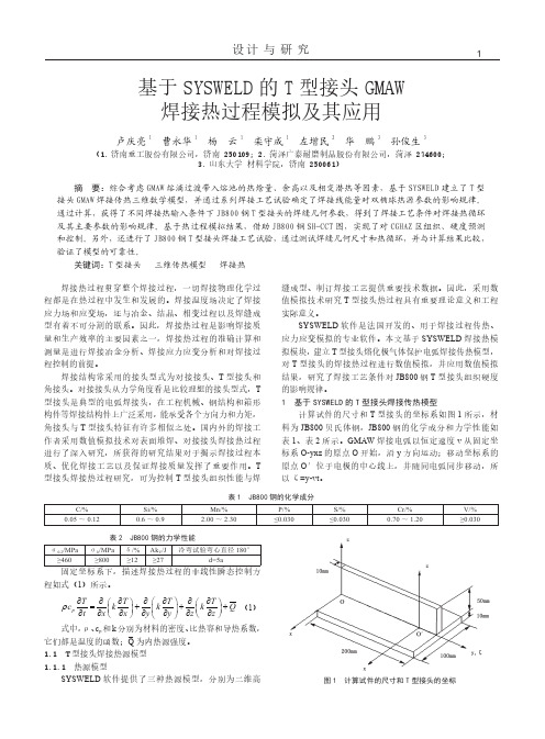
计算试件的尺寸和 T 型接头的坐标系如图 1 所示,材 料为 JB800 贝氏体钢,JB800 钢的化学成分和力学性能如 表 1、表 2 所示。GMAW 焊接电弧以恒定速度 v 从固定坐 标系 O-yxz 的原点 O 开始,沿 y 方向运动;移动坐标系的 原点 O′位于电极的中心线上,并随同电弧同步移动,所 以 ζ=y-vt。
反变形量对S355钢T型接头变形与残余应力影响的数值分析

反变形量对S355钢T型接头变形与残余应力影响的数值分析孙进发;刘明伟;刘海龙;杜文普【摘要】T型接头是一种应用较为广泛的焊接形式,其焊接过程中产生的焊接变形和残余应力将影响到结构的完整性和使用可靠性.为了抵消和补偿焊接变形,在进行焊接装配时,先在工件与焊接变形相反的方向进行人为变形,该方法称为反变形方法,是生产中最常用的方法之一.为研究反变形对焊后变形及残余应力的影响,基于热弹塑性法,以S355钢T型接头为研究对象,对其多层多道焊接变形与残余应力场进行数值模拟,并模拟了不同的反变形量.结果表明:S355钢T型接头焊后变形最大值出现在腹板远离焊缝一端;Von-Mises等效应力集中在焊缝区与热影响区.通过在腹板施加适当反变形,可在不影响整体残余应力峰值的情况下有效减小焊接变形,进而兼顾T型接头的平整度与承载能力.研究结果对实际焊接生产具有一定的指导意义.【期刊名称】《电焊机》【年(卷),期】2018(048)012【总页数】6页(P74-79)【关键词】T型接头;反变形;有限元法;焊接变形;残余应力【作者】孙进发;刘明伟;刘海龙;杜文普【作者单位】中车青岛四方机车车辆股份有限公司质量管理部,山东青岛266000;中车青岛四方机车车辆股份有限公司质量管理部,山东青岛266000;中车青岛四方机车车辆股份有限公司质量管理部,山东青岛266000;大连交通大学材料科学与工程学院,辽宁大连116028【正文语种】中文【中图分类】TG142;TG446;TP150 前言焊接由于方法经济、灵活,可简化结构细节,节约材料,提高生产效率[1],目前广泛应用于船舶、机车、车辆、桥梁、锅炉等工业领域,以及能源工程、海洋工程、航空航天工程、石油化工工程、大型厂房、高层建筑等重要结构。
T型接头是一种应用较为广泛的焊接形式,其焊接过程中发生的焊接变形和残余应力是影响焊接产品精度和性能的重要因素。
焊接变形及残余应力将影响到腐蚀、裂纹、疲劳强度等力学性能[2],同时也会对材料的物理机械性能产生巨大影响,对T型接头的强度造成很大危害。
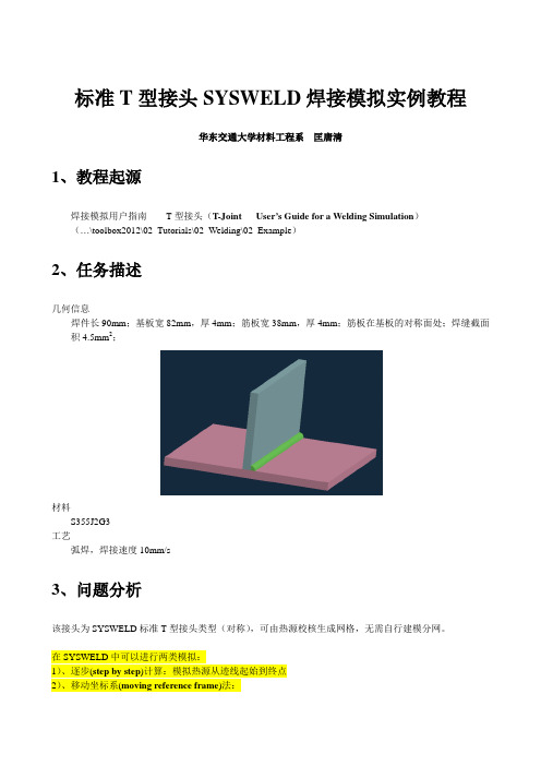
T型接头焊接模拟实例教程
OK,保存热源数据,并开始计算 在工作路径下产生材料金相属性文件 METALLURGY.DAT
4.2.5 结果查看
计算完后在工作路径 Input 下产生文件 HSF_DATA100.TIT, HSF_TRAN100.TIT, HSF_POST100.fdb 返回 Process 可发现 Qf 和 Qr(双椭球前后半球单位体积输入能量)根据输入的功率按原输入的比例 进行了相应调整
选 006-008,Display,显示 7.5s 时刻的热影响区形貌(006 为温度,007 为热影响区等值面,008 为几 何边界)
选 009-011,Display,显示 7.5s 时刻的截面温度(009 为温度,011 为几何边界)
4.2.6 热源校核
将模拟的焊缝与实际焊缝相对照,根据实际情况调整 Process 里面的参数(修改方法:点击 Process 下 面框中的文字,然后修改项的数据,修改后,点击 Replace 即可替换掉以前的值),修改后继续点击 OK 计 算,观察结果,直到焊缝的熔池及热影响区与实际情况相符合为止。确定热源参数后点击 Save 保存
在视图区看见该热源的效果,由此可见截面内熔池形状及热影响区大小。
查看后处理结果 PostprocessingTime-Space Functions 时-空函数 选择函数号 Function number 1000,要查看的时间 7.5s
OK 后可查看到 7.5s 时热源所在位置
PostprocessingPost DB…
4) 5)
进入热源校核界面 ApplicationWelding AdvisorToolsHeat Input Fitting
4.2.1 接头几何模型构建 4.2.1.1 2D 网格
课程设计——基于sysweld软件的T型接头焊接仿真模拟

——焊接基于sysweld软件的T型接头焊接仿真模拟姓名:000班级:材料000班学号:00000000指导老师:000日期:2011年09月SYSWELD——法国ESI公司的焊接仿真分析软件,经20多年发展,已成为热处理、焊接和焊接装配过程模拟的领先模拟软件,能够全面考虑材料特性、设计和过程的各种情况。
随着科学技术的发展,机械制造行业也随之不断的革新和进步。
人们对铸件的质量要求也越来越高,而SYSWELD为其提供了一个良好的工具,对提高铸件的质量有未雨绸缪的作用。
SYSWELD热过程模拟软件对铸件的制造起着非常关键的作用,为解决铸件缺陷问题提供了一个平台。
利用SYSWELD软件对焊缝进行计算机仿真模拟来提高焊缝的质量,本文主要对焊接的热过程模拟来分析T形接头焊焊接热过程,主要通过T形建模、热源校核、焊接向导、求解计算及结果后处理的操作步骤对焊接热过程进行数值模拟。
与测试并修正的传统方法相比,SYSWELD使得成本降低、周期缩短。
另外还能够显著减少物理样机,产生高的投资回报率。
界面友好,轻松易学。
SYSWELD 是用于引导工程师发现关于变形、残余应力和塑性应变的影响因素,然后优化过程参数的专业模拟软件。
2011-09-091、T型接头模型的建立1.1创建Points (1)1.2由Points生成Lines (1)1.3由Lines生成Edges (2)1.4由Edges生成Domains (2)1.5离散化操作 (3)1.6划分2D网格 (5)1.7生成Volumes (6)1.8离散Volumes (8)1.9生成体网格 (10)1.10划分换热面 (11)1.11划分1D网格 (12)1.12合并节点 (13)1.13保存模型 (14)1.14组的定义操作 (15)1.15保存 (17)1.16小结 (17)2、焊接热源校核2.1网格的建立 (18)2.2材料的导入及定义 (20)2.3热源过程参数的定义 (20)2.4求解 (21)2.5热源显示 (21)2.6修改参数 (22)2.7热源校核 (22)2.8检查显示结果 (23)2.9保存函数 (24)2.10热源查看 (24)2.11保存热源 (25)2.12小结 (25)3、焊接模拟向导设置3.1材料的导入 (26)3.2热源的导入 (26)3.3材料的定义 (27)3.4焊接过程的定义 (27)3.5热交换的定义 (28)3.6约束条件的定义 (28)3.7焊接过程求解定义 (28)3.8冷却过程求解定义 (29)3.9检查 (29)3.10小结 (31)4、后处理与结果显示分析4.1计算求解 (32)4 .2导入后处理文件 (32)4.3结果显示与分析 (33)4.4小结 (36)1、T型接头模型的建立1.1创建Points根据所设计T型接头模型的规格,选定原点,然后分别计算出各节点的坐标,按照Geom./Mesh.→geometry→point步骤,建立以下13个点:P1(-25,0,-10)、P2(7,0,-10)、P3(10,0,-10)、P4(13,0,-10)、P5(35,0,-10)、P6(35,0,0)、P7(10,0,0)、P8(10,0,30)、P9(0,0,30)、P10(0,0,3)、P11(-1.5,0,1.5)、P12(-3,0,0)、P13(-25,0,0)如下图所示:1.2由Points生成Lines按照Geom./Mesh.→geometry→1Dentities步骤,按照一定的方向性将各点连接成如下图所示的Lines:1.3由Lines生成Edges按照Geom./Mesh.→geometry→EDGE步骤,点击选择各边,依次生成如下图所示各Edges:1.4由Edges生成Domains按照Geom./Mesh.→geometry→Domains步骤,依次生成如下六个Domains:1.5离散化操作离散化操作是针对由Points所生成的Lines而言,由于除了有这些点生成的线以外,软件本身也会自动产生一些辅助的线条,为了方便清晰地对所生成的主要线条进行选取及其他操作,可以通过“隐藏→显示”处理,只显示如下图所示的十八条线:通过以下操作为后面的离散操作做好准备:→通过Meshing→Definition→Discretisation启动离散化操作界面,将L2、L4、L8、L10四条线均匀离散成3段,将其他十四条线非均匀离散,离散单元数为5,系数为3.5。
基于Sysweld的焊接接头热源模型二次开发
1.2 热源模型 Sysweld 软件内置了 3 种结构简单的热源模型[6],
20 ·试验与研究·
分别为:
(1) 二维高斯面热源模型, 适用于表面热处理;
(2) 三维高斯锥形热源 模 型 , 适 用 于 激 光 焊 、
电子束焊等高能束流焊接;
(3) 三维双椭球热源模型, 适用于 TIG, MIG 焊
1.3 热源计算
基于 Sysweld 平台开发自定义的异型焊 接 接 头 ,
建立三维有限元模型, 其单元类型、 单元组的数量
和种类必须和内置的热源模型一致, 具体包括:
(1) 建立包含焊缝和母材的 3D 单元组; (2) 从 3D
单元抽取表面网格, 生成 2D 单元组, 表征换热面;
(3) 从焊缝和母材的 3D 单元沿着焊接方向抽取 2 条
摘要: 焊接接头的结构形式和尺寸精度直接影响热源模型计算结果的准确性 , 工程实际应用的焊接接头形式多样、 结构复杂, Sysweld
内置的焊接接头远不能满足实际需求。 基于 Hypermesh, Sysweld 软件平台开发了大坡口角焊缝和双侧多层角焊缝热源模型, 首先利用
Hypermesh 建立有限元模型生成可执行的内嵌文件, 利用 Sysweld 的 HSF 工具反复调整 双 椭 球 热 源 高 斯 参 数 , 并 将 校 核 结 果 与 试 验 结
1 大坡口角焊缝的热源计算 1.1 几何模型
焊接结构的接头形式和形状多种多样, 只利用 专用商业焊接有限元软件所提供的自定义接头往往 不够, 这就要求必须根据工程实际自定义接头形式 和形状。 如图 1 所示的大坡口角焊缝, 其坡口位置、 坡口角度直接影响传热过程, 继而影响焊接结构件 最终的变形量和组织性能。
chap5 SYSWELD焊接模拟范例——T型接头
5
模拟流程
3 – 通过Welding Wizard焊接向导定义焊接问题
应输入以下数据
组件材料属性参数 移动热源(迹线、速度、强度) 热/力边界条件 初始温度和材料组织成分 求解器参数
借助材料库、函数库和专用组名来建立要求解的问题 所有输入数据都存放在工程文件中,可导入、修改和保 存
Copyright © ESI Group, 2012. All rights reserved.
39
1 6 2 4
3 5
Copyright © ESI Group, 2012. All rights reserved.
40
热影响区
熔融区
Copyright © ESI Group, 2012. All rights reserved.
94
1
Perform the solution of the problem
模拟的稳态计算部分在当前的PC机上需约半小时
95
重启瞬态计算以模拟 焊接结束时及冷却
96
1 2 3
97
1 – 重启过程restart procedure名, 对第一个重启名为 projectName-1, 第二个重启名为ProjectName-2, 以此类推
6
模拟流程
模拟向导会话保存后:
从材料库和函数库中提取出所需要的材料 属性和函数 得到可由求解器解析的命令文件 <PROJECT_NAME>_*.DAT (也称“工程 文件 ” ) ,该文件包括材料属性应用、载 荷和网格约束以及问题求解顺序。
7
模拟流程
4 – 问题的有限元求解
T形接头焊接温度场的三维数值模拟

Welding Technology Vol.37No. 6Dec . 2008T 形接头焊接温度场的三维数值模拟熊震宇 1, 董洁 2(南昌航空大学材料科学与工程学院 , 江西南昌 330063摘要 :利用有限元分析软件 ANSYS , 对 T 形接头焊接的温度场的分布进行了动态模拟 , 提出高斯函数和双椭球函数相结合的双热源模型。
并应用 APDL 语言实现了焊接全过程温度场的三维动态模拟 , 其结果与理论值完全吻合 , 证明了数值模拟的可靠性。
关键词 :T 形接头 ; 焊接 ; 数值模拟 ; APDL ; 温度场中图分类号 :TG445文献标识码 :B文章编号 :1002-025X (200806-0021-03焊接热过程数值模拟是焊接数值模拟的一个主要方面 , 它把焊接学科与计算机技术结合在一起 , 为定量地研究焊接冶金起到积极的推动作用 [1]。
ANSYS 软件是以有限元分析为基础的大型通用 CAE 软件 , 其强大的热结构耦合及瞬态、非线性分析能力使其在焊接模拟技术中具有广阔的应用前景 [2]。
本文研究利用 ANSYS 软件的参数化程序语言 APDL 编制了焊接过程三维瞬态温度场模拟分析程序 , 并以 T 形接头埋弧焊为例给出了具体分析过程 , 计算结果与理论结果比较吻合。
1有限元模型的建立本文所选用的模型为 :腹板尺寸 60mm ×16mm ×100mm , 翼板尺寸 100mm×20mm ×100mm , 材料为 Q345。
T 形接头模型如图 1所示。
为了描述 T 形接头三维焊接温度场的分布 , 热分析单元中选取单元 SOLID87, 在加热圆弧面上生成无中间节点的三维 4节点弧形的表面效应单元SURF152。
如图 2所示 , 在焊缝区域及近缝区采用细网格 , 而远离焊缝区采用较粗的网格。
热源沿着 T 形接头 z 轴的方向匀速移动。
1.1热源模型焊接热源具有局部集中、瞬时和快速移动的特点 , 在时间和空间域内都易形成梯度很大的不均匀温度场是进行焊接力学分析的基础 , 而焊接温度场模型的精确性依赖于热源模型的精度 , 因而建立一个合适的焊接热源模型是焊接模拟过程中的重要部分。
SYSWELD 教程

一、计算数据材料:516-GRADE-70,熔点1430摄氏度,最小抗拉强度极限为70ksi (485Mpa),为中温及低温压力容器用钢,成分C≤12.5 Si≤0.27Mn≤0.15-0.40 P≤0.85-1.20 S≤0.035 Cu≤0.035 Ni≤0.40 Cr≤0.40 Mo≤0.30V≤0.12Nb≤0.03Ti ≤0.02Al≤0.03,相当于国内16MnRD(GB3531-2008 )。
尺寸:两块相同板35mm*80mm*3mm,热源双椭球尺寸:5*10*5*2功率:2000w二、接头模型的建立2.1 创建点根据所设计的对接接头模型的规格,分别计算出各节点的坐标,按照Geom./Mesh.→geometry→point 步骤,建立以下10个点:P1(0,0,0),P2(8,0,0),P3(35,0,0),P4(35,0,-3),P5(8,0,-3),P6(0,0,-3),P7(-8,0,-3),P8(-35,0,-3),P9(-35,0,0),P10(-8,0,0),如图所示:2.2 有Point生成lines按照Geom./mesh→geometry→1D entities步骤,按照一定的方向性将各点连接成如下图所示的Lines:2.3 由lines 生成Edges按照Geom./mesh→geometry→EDGE 步骤,点击选择各边,依次生成如下图所示各Edges:2.4 由Edges 生成domains按照Geom./mesh→geometry→Domains→edges 步骤,依次生成如下Domains:2.5 离散化操作可以通过display→erase隐藏,entries→show显示,“隐藏→显示”处理,只显示13 条线。
通过以options→display→mode→点亮discretisation,为离散化做准备。
通过Meshing→Defintion→D iscretisation 启动离散化操作界面,讲各条线进行离散,实例中将L9、L10、L11、L12、L13 五条线均匀离散成3 段,L1、L3、L5、L7 均匀离散成10 段,将剩余L2、L4、L6、L8条线非均匀离散,最小尺寸为1,最大为3。
SYSWELD焊接仿真入门教程

输入工作名 及注释
打 开 Welding Wizard 焊接向导
QQ2361566926
加载材料库
材料库 点击加载
加载函数库
建立节点 Nodes
Node 菜单 by XYZ locate 建立节点坐标
生成面 surface
Surface 菜单 Blend(Spline)生成面
生成 2D mesh
2D 菜单 Auto mesh Surfaces 生成 2D 网格
拉伸 3D mesh
3D 菜单 Sweep(Drag)拉伸生成 3D 网格
到目前完成了焊接模拟的前处理过程,即焊接过程的所有要素都被转化成了 可以在求解过程中能够被识别的网络,现在需要将 visual-mesh 建立的模型保存 为 Sysweld 所识别的格式,ASC 文件。命名格式为**_DATA**.ASC,其中 DATA 前面是下横杠,DATA 后面是数字,下横杠前面是自己的名称,所建模型如下图。
15
(4) 最小网格尺寸
1
(5) 最大网格尺寸
3
输入后点击Save,进行保存,生成三维网格如下图。
QQ2361566926
选择选项
3.2 加载材料数据库及函数数据库 Material DB是材料数据库的意思,这里面存储了材料的热物性参数、热力学
数据、相变参数等等。
1 材料数据 库
2 点击加载
3 默认安装 路径下的材 料库文件 welding.mat
热交换选择
热交换定义 模块
solidworks网格划分技巧
CosmosWorks网格划分、求解器、提示与技巧一、网格划分策略网格划分,更精确地说应该称为离散化,就是将一数学模型转化为有限元模型以准备求解。
作为一种有限元方法,网格划分完成两项任务。
第一,它用一离散的模型替代连续模型。
因此,网格划分将问题简化为一系列有限多个未知域,而这些未知域符合由近似数值技术的求解结果。
第二,它用一组单元各自定义的简单多项式函数来描述我们渴望得到的解(e.g位移或温度)。
对于使用者来说,网格划分是求解问题必不可少的一步。
许多FEA初学者急切盼望格划分为全自动过程而几乎不需要自己输入什么。
随着经验的增加,就会意识到这样一个现实:网格划分常常是要求非常苛刻的任务。
商用FEA软件的发展历史见证了网格划分对F EA 用户透明的诸多尝试,然它并不是一条成功的途径。
而当网格划分过程既简单又自动执行时,它也仍旧不是一个“非手工干涉”而仅靠后台运行的任务。
作为FEA用户,我们想要有一种可以和网格划分过程交互的方法。
COSMOSW orks通过将用户从那些纯粹网格细节意义上的问题中解脱出来,找到了良好的平衡点;并使我们在需要时可以控制网格划分。
几何体准备理想情况下,我们用SolidW orks的几何体,联入COSMOSWorks环境。
在这里,我们定义分析和材料的类型,施加载荷与约束,然后为几何体划分网格并得到求解。
这种方法在简单模型下能起作用。
对于更为复杂的几何体,则要求在网格划分前作些准备。
在FEA 的几何体准备过程中,我们从特定制造,CAD 几何体出发,为分析而特地构造几何体。
我们称这个几何体为FE A 几何体。
基于两者的不同要求,我们对CAD 几何体和FE A 几何体作一区别:CAD 几何体FEA几何体必须包含机械制造所需的所有信息必须可划分网格必须允许创建能正确模拟所关心资料的网格必须允许创建能在合理时间内可求解的网格通常,CAD 几何体不能满足FEA 几何体的要求。
SYSWELD 教程
一、计算数据材料:516-GRADE-70,熔点1430摄氏度,最小抗拉强度极限为70ksi (485Mpa),为中温及低温压力容器用钢,成分C≤12.5 Si≤0.27Mn≤0.15-0.40 P≤0.85-1.20 S≤0.035 Cu≤0.035 Ni≤0.40 Cr≤0.40 Mo≤0.30V≤0.12Nb≤0.03Ti ≤0.02Al≤0.03,相当于国内16MnRD(GB3531-2008 )。
尺寸:两块相同板35mm*80mm*3mm,热源双椭球尺寸:5*10*5*2功率:2000w二、接头模型的建立2.1 创建点根据所设计的对接接头模型的规格,分别计算出各节点的坐标,按照Geom./Mesh.→geometry→point 步骤,建立以下10个点:P1(0,0,0),P2(8,0,0),P3(35,0,0),P4(35,0,-3),P5(8,0,-3),P6(0,0,-3),P7(-8,0,-3),P8(-35,0,-3),P9(-35,0,0),P10(-8,0,0),如图所示:2.2 有Point生成lines按照Geom./mesh→geometry→1D entities步骤,按照一定的方向性将各点连接成如下图所示的Lines:2.3 由lines 生成Edges按照Geom./mesh→geometry→EDGE 步骤,点击选择各边,依次生成如下图所示各Edges:2.4 由Edges 生成domains按照Geom./mesh→geometry→Domains→edges 步骤,依次生成如下Domains:2.5 离散化操作可以通过display→erase隐藏,entries→show显示,“隐藏→显示”处理,只显示13 条线。
通过以options→display→mode→点亮discretisation,为离散化做准备。
通过Meshing→Defintion→D iscretisation 启动离散化操作界面,讲各条线进行离散,实例中将L9、L10、L11、L12、L13 五条线均匀离散成3 段,L1、L3、L5、L7 均匀离散成10 段,将剩余L2、L4、L6、L8条线非均匀离散,最小尺寸为1,最大为3。
T型接头焊接温度场ANSYS仿真分析
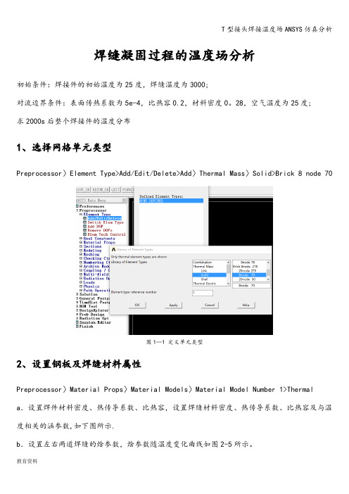
焊缝凝固过程的温度场分析初始条件:焊接件的初始温度为25度,焊缝温度为3000;对流边界条件:表面传热系数为5e-4,比热容0.2,材料密度0。
28,空气温度为25度;求2000s后整个焊接件的温度分布1、选择网格单元类型Preprocessor〉Element Type>Add/Edit/Delete>Add〉Thermal Mass〉Solid>Brick 8 node 70图1—1 定义单元类型2、设置钢板及焊缝材料属性Preprocessor〉Material Props〉Material Models〉Material Model Number 1>Thermal a.设置焊件材料密度、热传导系数、比热容,设置焊缝材料密度、热传导系数、比热容及与温度相关的涵参数,如下图所示.b.设置左右两道焊缝的焓参数,焓参数随温度变化曲线如图2-5所示。
图2—1 钢板热导率设置图2—2 设置钢板比热容图2-3 设置钢板密度图2—4 焊缝焓参数设置图2—5 左右焊缝焓参数3、建立几何模型Preprocessor〉Modeling>Create>Volumes>Block〉By Dimensions 建立焊件几何模型。
Preprocessor〉Modeling>Create〉Volumes>Cylinder>By Dimensions 建立焊缝几何模型。
建模过程如图3-1所示。
图3—1 几何模型建模过程1图3-2 几何模型建模过程2通过Reflect建立完整的几何模型,之后运用布尔运算中glue使整个模型成为一个整体,如图3-3所示.焊接模型几何参数:横板:2*1.2*0。
4竖板:0。
4*1.2*1焊缝:R0.2*1。
2图3-3 焊件几何模型设置焊件及左右焊缝网格属性Preprocessor〉Meshing>Mesh Attributes〉Picked 选择焊件或是焊缝,分别对其进行设置。
基于SYSWELD的搭接接头温度场的数值模拟
基于SYSWELD的搭接接头温度场的数值模拟张书权;王仲珏;朱协彬;代礼;文伟【期刊名称】《新乡学院学报(自然科学版)》【年(卷),期】2010(027)006【摘要】基于有限元软件SYSWELD对搭接接头温度场进行了3维动态模拟,得出了瞬态温度场分布图和特征点的热循环曲线.同时通过对SYSWELD后处理分析,得出了焊件上任一点的温度变化与相演变的关系.与文献资料比较表明,所建立的数值模拟仿真模型可以较好地模拟焊接温度场,为研究焊接过程中的应力应变和减少焊接应力与变形提供了参考依据.【总页数】3页(P67-69)【作者】张书权;王仲珏;朱协彬;代礼;文伟【作者单位】安徽工程大学,机械与汽车工程学院,安徽,芜湖,241000;安徽机电职业技术学院,机械工程系,安徽,芜湖,241000;安徽工程大学,机械与汽车工程学院,安徽,芜湖,241000;安徽工程大学,机械与汽车工程学院,安徽,芜湖,241000;安徽机电职业技术学院,机械工程系,安徽,芜湖,241000;中国科学院,等离子体物理研究所,安徽,合肥,230000【正文语种】中文【中图分类】TG402【相关文献】1.基于SYSWELD的搭接接头温度场的数值模拟 [J], 张书权;王仲珏;朱协彬;代礼;文伟2.基于SYSWELD软件T型接头焊接温度场的数值模拟分析 [J], 陈俊安;崔建峰;李峰超;王乐;赵宏伟3.基于SYSWELD的X80管线钢焊接接头温度场的数值模拟 [J], 田万鹏4.基于SYSWELD软件T型接头焊接温度场的数值模拟分析 [J], 陈俊安;崔建峰;李峰超;王乐;赵宏伟5.基于SYSWELD的铝合金厚板多层多道焊焊接温度场和焊接变形的数值模拟 [J], 杨仲林;王陆钊;鲁二敬;李充;于岩因版权原因,仅展示原文概要,查看原文内容请购买。
- 1、下载文档前请自行甄别文档内容的完整性,平台不提供额外的编辑、内容补充、找答案等附加服务。
- 2、"仅部分预览"的文档,不可在线预览部分如存在完整性等问题,可反馈申请退款(可完整预览的文档不适用该条件!)。
- 3、如文档侵犯您的权益,请联系客服反馈,我们会尽快为您处理(人工客服工作时间:9:00-18:30)。
Visual-MeshV3.0Tutorial 13:CAD for ‘T’ Weld JointVTS-3.0-ME-AT-12This working document and related know-how herein provided by ESI Group subject to contractual conditions are to remain confidential. The client shall not disclose the documentation and/or related know-how in whole or in part to any third party without the prior written permission of ESI GroupCopyright © ESI Group, 2007. All rights reserved.Prerequisites:It is recommended to have familiarity with the basic features of Visual Mesh.Objective:In this tutorial you will learn how to use Surface and Curve options in Visual Mesh effectively to created CAD model which will represent a Weld JointDescription:In Visual Mesh there are many CAD (Surfaces and Curves) generation and editing methods. We have send some of the CAD editing features in previous tutorials. In the following tutorial you will learn to generate Surfaces and Curves on a new model which will be representation of the weld model, a ‘T’ Joint.Outline:Loading Model ............................................................................... 错误!未定义书签。
Ground Plate Modeling................................................................. 错误!未定义书签。
Rib Modeling .................................................................................. 错误!未定义书签。
Filler Material ModelingGap ModelingCurves GenerationParts ManagementSaving the ModelDuration:This tutorial will take approximately 25 minutes to execute.Files used:This tutorial uses a new model, Document1.vdbLoading Model•Invoke Visual-Mesh.•Click File -> New or press CTRL+N Files•New model window will start with the default name of Document1.vdbGround Plate ModelingNodes Creation•Post By XYZ, Locate… GUI from Nodes menu (Nodes -> By XYZ, Locate…) or hit F8 key•With default Node creation method, in the posted GUI enter the 0, -60,10 in the X, Y & Z fields respectively• The default method will be XYZ and the default ID 1 for the new Node.Click on Create Node and see in the model window that there will be a new node.•For Node 2, enter 0, 60, 10 in the X, Y, Z fields and click on Create Node.•For Node 3, enter 0, -60, 0 in the X, Y, Z fields and click on Create Node.•For Node 4, enter 0, 60, 0 in the X, Y, Z fields and click on Create Node.•The new nodes will have IDs of 1, 2, 3 and 4 respectively.•Close the By XYZ, Locate…To Create a Surfaces with the required size, you need to create Nodes. With the help of these nodes Surface and curves will be created.Surface Creation by Blend•Post Blend GUI from Surface menu (Surface -> Blend (Spline) )•Change Mesh only option to Surf Only option•In the model window pick Node 1 & Node 2 and confirm by middle mouse button. This becomes first primary edge for the blend Surface. •Pick Node 3 & Node 4 and confirm by middle mouse button. This becomes second primary edge for the blend Surface.•Click on OK to confirm. The new surface will be created and it will be in Part 1 which is default.Surface Creation by Sweep•Post Sweep GUI from Surface menu (Surface -> Sweep (Drag) )•Change sweeping curve option to Multiple Curves and enter 200 in the Distance field.•Change Mesh only option to Surf Only option•Enter 1 in Part ID filed•Pick the top edge of the newly created Surface as shown in the below picture and confirm•After confirming the sweep curve selection, a Vector Definition GUI is posted•Select Global Axis as the Vector definition option and click on Flip to make the vector in - X direction•Click on Ok/Close in the Vector Definition GUI to accept the Vector and close the GUI•Look the preview of the surface to be generated and confirm it by clicking on Ok in Sweep GUIFollow the same above steps and generate 3 more sweep surfaces by selecting the remaining 3 edges of the blend surface. 1 Blend surface and 4 Sweep surfaces will look like as shown in the picture below.Now you need to copy the Blend surface on the other ends of the Sweep surfaces to represent the closed volume of the Ground plateSurface Transform•Post Surface Transform GUI from Surface menu (Surface -> Transform)•Toggle on Fix option for Y Axis and Z Axis and enter -200 in the dX field•Select the Surface created by blend and confirm by clicking on Update Entities•Toggle Copy option and keep the other options default•Confirm the transformation by Clicking on CopyThis completes the modeling of the Ground plate. Now we will model the Rib Plate.Rib ModelingNodes Creation•Post By XYZ, Locate… GUI from Nodes menu (Nodes -> By XYZ, Locate…)•With default Node creation method, in the posted GUI enter the 0, -5,12 in the X, Y & Z fields respectively. The ID of the new Node will be 5.•Click on Create Node and see in the model window that there will be a new node.•For Node 6, enter 0, -5, 72 in the X, Y, Z fields and click on Create Node.•For Node 7, enter 0, 5, 12 in the X, Y, Z fields and click on Create Node.•For Node 4, enter 0, 5, 72 in the X, Y, Z fields and click on Create Node.•The new nodes will have IDs of 5, 6, 7 and 8 respectively.•Close the By XYZ, Locate…Surface Creation by Blend•Post Blend GUI from Surface menu (Surface -> Blend (Spline) )•Change Part ID as 2 and keep other options default•For first primary, pick Node 5 & Node 6 and confirm by middle mouse button.•Pick Node 7 & Node 8 and confirm by middle mouse button. This becomes second primary edge for the blend Surface.•Click on OK to confirm. The new surface will be created and it will be in Part 2Surface Creation by Sweep•Post Sweep GUI from Surface menu (Surface -> Sweep (Drag) )•Make sure that the default options in the GUI are Multiple Curves, Distance 200 and Part ID 2.•Pick one edge of the blend surface created in the previous step•When Vector Definition panel is posted see that the default option method will be Global Axis with X – Axis. If required use Flip option to get the surface as shown in below pictureFollow the same above steps and generate 3 more sweep surfaces by selecting the remaining 3 edges of the blend surface. 1 Blend surface and 4 Sweep surfaces will look like as shown in the picture belowSurface Transform•Post Surface Transform GUI from Surface menu (Surface -> Transform)•Toggle on Fix option for Y Axis and Z Axis and enter -200 in the dX field•Select the Surface created by blend of Part 2 and confirm by clicking on Update Entities•Toggle Copy option and keep the other options default•Confirm the Surface transform by clicking on Copy in the GUI and close the GUIThis completes the modeling of the Rib plate. Now we will model the Weld Bead.Filler Material ModelingNodes Creation•Post By XYZ, Locate… GUI from Nodes menu (Nodes -> By XYZ, Locate…) or hit F8 key•With default Node creation method, in the posted GUI enter the 0, 5,16 in the X, Y & Z fields respectively. The ID of the new Node will be 5.•Click on Create Node and see in the model window that there will be a new node.•For Node 6, enter 0, 5, 10 in the X, Y, Z fields and click on Create Node.•For Node 7, enter 0, 11, 10 in the X, Y, Z fields and click on Create Node.•The new nodes will have IDs of 9, 10 and 11 respectively.•Close the By XYZ, Locate… GUISurface Creation by Blend•Post Blend GUI from Surface menu (Surface -> Blend (Spline) )•Change Part ID as 3 and hit Enter and keep other options default •For first primary, pick Node 9 & Node 10 and confirm by middle mouse button.•Pick Node 11 & Node 10 and confirm by middle mouse button. This becomes second primary edge for the blend Surface.•Click on OK to confirm. The new surface will be created and it will be in Part 3Surface Creation by Sweep•Post Sweep GUI from Surface menu (Surface -> Sweep (Drag) )•Make sure that the default options in the GUI are Multiple Curves, Distance 200 and Part ID 3.•Pick one edge of the blend surface created in the previous step•When Vector Definition panel is posted see that the default option method will be Global Axis with X – Axis. If required use Flip option to get the surface as shown in below picture•Follow the same above steps and generate 2 more sweep surfaces by selecting the remaining 2 edges of the blend surface.Surface Transform•Post Surface Transform GUI from Surface menu (Surface -> Transform)•Toggle on Fix option for Y Axis and Z Axis and enter -200 in the dX field•Select the Surface created by blend of Part 3 and confirm by clicking on Update Entities•Make a Copy of the surfaces at the other end. It should be as like done for the Ground PlateThis finishes modeling of the Filler Material. Now you will model the Chewing Gum materialGap material ModelingNodes Creation by Node Drop•Change Entity Selector to Nodes and click on the Disp ID icon. See the picture below•Select all the nodes and see that all the nodes IDs are displayed in the model window•Remove the Node Selection by hitting ESC key or clicking on hitting CTRL+D•Post Drop Points/Curves/ Nodes GUI from Nodes menu.(Nodes -> Drop (Project))•With all defaults options, select the Node 5 (N -5) and confirm by middle mouse button or click on Update Entities•Click on Select Surfaces and pick the top surface of the Ground Plate•Change the Move option to make a Copy•Confirm the Copying of the Node by clicking on OK and close the GUI. Surface Creation by Blend•Post Blend GUI from Surface menu (Surface -> Blend (Spline) )•Change Part ID as 4 and hit Enter and keep other options default •For first primary, pick Node 5 & Node 7 and confirm by middle mouse button.•Pick Node 12 & Node 10 and confirm by middle mouse button. This becomes second primary edge for the blend Surface.•Click on OK to confirm. The new surface will be created and it will be in Part 4Surface Creation by Sweep•Post Sweep GUI from Surface menu (Surface -> Sweep (Drag) )•Make sure that the default options in the GUI are Multiple Curves, Distance 200 and Part ID 4.•Pick one edge of the blend surface created in the previous step •When Vector Definition panel is posted see that the default option method will be Global Axis with X – Axis. If required use Flip option to get the proper surfaces between the Rib and the Ground Plate •Follow the same above steps and generate 3 more sweep surfaces by selecting the remaining 3 edges of the blend surface.Surface Transform•Post Surface Transform GUI from Surface menu (Surface -> Transform)•Toggle on Fix option for Y Axis and Z Axis and enter -200 in the dX field•Select the Surface created by blend of Part 4 and confirm by clicking on Update Entities•Make a Copy of the surfaces at the other end. It should be as like done for the Ground Plate or the RibThis finishes modeling of the Gap modeling and also modeling of all the surfaces.Now you need to model the curves which will be used to represent the different heat zones of the weld model. For this once again display the IDs of all the nodes.Curves GenerationNodes Transform•Post Nodes Transform GUI from Nodes Menu (Nodes -> Transform)•Select the Node 12 and confirm by middle mouse button on click on Update Entities•In the posted GUI, Fix X and Z axis. Enter -10 in the dY field and toggle on the Copy option•Copy the node by clicking on button Copy•Similarly select the Node 11 and confirm by middle mouse button on click on Update Entities•Fix X and Z axis. Enter 10 in the dY field Copy the node by clicking on Copy•select the Node 9 and confirm by middle mouse button on click on Update Entities•Fix X axis and Y axis, free the Z Axis. Enter 10 in the dZ field Copy the node by clicking on Copy•The new Nodes will have the IDs 13, 14 & 15.Nodes Creation by Node Drop•Post Drop Points/Curves/ Nodes GUI from Nodes menu.(Nodes -> Drop (Project))•With all defaults options, select the Nodes 10, 11, 12, 13 & 14 (all nodes at the Top Edge of the Ground Plate)and confirm by middlemouse button or click on Update Entities•Click on Select Surfaces and pick the bottom surface of the Ground Plate•Make sure that the option is to make a Copy of nodes•Confirm the Copying of the Node by clicking on OK.•Select Nodes 9 & 15 and confirm.•Select the back surface of the Rib to drop the nodes on it as shown in the below picture.•Confirm the Copying of the Node by clicking on OK and close the GUI Node AlignTo make sure that the dropped nodes are on the edge of the face, use align node option•Post Align Nodes/Elem. Edges GUI from Node menu (Node -> Align)•Change option Curve to align•Pick the edge of the surface on which the nodes are lying. It will be highlighted.•Now pick all the nodes on that edge and confirm.•Do the same for all the edges where the nodes are located. This is to insure that the nodes are indeed on the edge.Creating Curve by Sketch•Post Sketch GUI from Curve menu (Curve -> Sketch)•With all the default options pick the pairs of nodes that are original and copied by drop options in the earlier step•See the below picture for the curves to be created in the below picture •Once the pair of nodes is selected confirm by middle mouse button to accept the created Curve.•Make sure that the Curves will be in Part 5Note: To make sure the picked point is on the Node only follow the below procedure.•Pick the first node for the first Curve. It shows the point handle by Curve (a Mark)•Once again click on the same node or the Point handle; it posts a point definition GUI as shown below.•Click on Node in the Snap to option and pick the same node.•This will insure that from here onwards if the point is picked near the node, it will get snapped to the node.Nodes Creation between Points•Fit the model in the w indow by hitting ‘F’ Key•Change the Display Mode by clicking on the icon•Post Between 2 Points GUI from Nodes menu.(Nodes -> Between 2 Points)•Toggle of Nodes at Ends option and enter 1 for Number of Nodes• Pick the nodes 2 & 14 to create Node 23. Similarly create Node 24 and 25.•See the below picture for the nodes to be createdNodes Creation by Transform•Post Node Transform GUI from Nodes menu (Nodes -> Transform)•Fix: Y Axis and Z Axis and keep only option to Copy the nodes in X Axis•Enter -200 in dX field and make sure that the Copy option is on.•Select Nodes 25, 13, 14, 23, 15 and 24 and confirm by middle mouse button. (See the above picture)•Click on Copy and close the GUINode AlignTo make sure that the transformed nodes and the original nodes are onthe edge of the face, use align node option. The procedure has to be followed as earlier.•Post Align Nodes/Elem. Edges GUI from Node menu (Node -> Align) •Change option Curve to align•Pick the edge of the surface on which the nodes are lying. It will be highlighted.•Now pick all the nodes on that edge and confirm.•Do the same for all the edges where the nodes are located. This is to insure that the nodes are indeed on the edge.Creating Curve by Sketch•Post Sketch GUI from Curve menu (Curve -> Sketch)•Change the Part ID to 6 for the new Curves.•With all the default options pick the pairs of nodes that are original and copied by drop options in the earlier step•All the new curves should be parallel to Global X Axis•Once the pair of nodes is selected confirm by middle mouse button to accept the created Curve.Parts ManagementWhen the entities are generated in different parts, the Parts are created with the default name. With the help of Part Manager we need to give proper names to the parts.•Post Part Manager from Assembly Menu or simply by hitting F11•In the NAMES column, click on the default name for the part and change the part name accordingly.See the below Part Manager with the part names to be givenCross check the Explorer for the names of the Parts as entered in the Part ManagerSaving the ModelThe model can be saved in different formats.To save VDB format•In the main menu, click File -> Save as …•Choose the path and the file name as T-Joint.vdb and confirmTo Export the Model in IGES format•In the main menu, click File -> Export…•Choose the path and the file name as T-Joint.igs and confirmThe free nodes that we have in the model were only for the modeling purpose. Thesenodes now can be deleted before saving the modelVisual-MeshV3.0This working document and related know-how herein provided by ESI Group subject to contractual conditions are to remain confidential. The client shall not disclose the documentation and/or related know-how in whole or in part to any third party without the prior written permission of ESI GroupCopyright © ESI Group, 2007. All rights reserved.Prerequisites:Execute the Tutorial 13 and also it is recommended to have familiarity with the basic features of Visual Mesh.Objective:In this tutorial you will learn how to create 1D, 2D & 3D mesh with the use of Surface and Curve using Visual Mesh which should be applicable for Welding JointDescription:The requirement for the weld joint mesh is to have very fine elements at the heat affected zone. And also as the region falls away from the Heat zone, the mesh should get coarsen. There should least number of elements with very fine elements at and near the Filler Material. This makes structured mesh for the weld joint. This tutorial give s the way to mesh a ‘T’ Weld Joint.Outline:Loading Model ............................................................................... 错误!未定义书签。