一种由Matlab仿真控制的自主移动机器人模拟器(英文)
RAMSIS简介

RAMSIS介绍RAMSIS是德语“Rechnergestütztes Anthropologisch-Mathematisches System zur Insassen-Simulation”的缩写,意思是“用于乘员仿真的计算机辅助人体数字系统”。
RAMSIS是一种用于乘员仿真和汽车人机工程设计的高效CAD工具。
该软件为工程师提供了一个详细的CAD人体模型,来模拟仿真驾驶员的行为。
它使设计者在产品开发过程的初期,在只有CAD数据的情况下就可以进行大量的人机工程分析,从而避免在以后阶段进行昂贵的修改设计。
RAMSIS在上个世纪80年代由德国凯泽斯劳腾的TECMATH股份有限公司(现在的Human Solutions股份有限公司)联合慕尼黑工业大学的人机工程学系开发。
初期RAMSIS的开发由整个德国汽车工业发起并资助。
他们的目标是,克服现存大多数二维人机工程工具SAE J826模板等的不足,在法规规定的基础上进一步提高车辆的人机工程品质。
RAMSIS已经成为汽车工业用于人机工程设计的全球标准。
目前已经被全球70%以上的轿车制造商所使用,包括Audi,Volkswagen,BMW,Porsche,DaimlerChrysler,Ford,General Motors,Honda,Mazda,Opel,Renault,Peugeot,Citro?n,Rover,Saab,Volvo,Daewoo,Seat,Skoda和Fiat等等。
其中,在中国的顾客有泛亚汽车技术中心、上海大众、上海汽车、上汽乘用车、一汽大众、一汽汽研、一汽轿车、华晨金杯、奇瑞、长安汽车、上汽五菱、北汽福田、北汽研究院、海南马自达、东风汽车等。
卡车,客车,叉车等工业用车制造商,如Freightliner和Iveco、MAN Commercial Vehicles、The Liebherr Werk Ehingen GmbH等也正在使用RAMSIS。
基于Matlab和Adams的自平衡机器人联合仿真

基于Matlab和Adams的自平衡机器人联合仿真徐建柱;刁燕;罗华;高山【摘要】为检验自平衡机器人控制系统的准确性及其动静态性能,采用Matlab/Simulink和Adams建立虚拟样机系统的方法.通过建立机器人的状态空间方程并利用LQR方法配置系统极点,设计出状态反馈控制器.分别在Simulink和Adams中建立机器人的控制系统和机械仿真模型,利用二者实现对机器人的联合仿真.仿真结果表明,所设计的控制方法能实现机器人平衡,并具有良好的动静态性能.%In order to test the accuracy and the static-dynamic characteristics of the control system of self-balance robots, a virtual prototype system was created based on Matlab/Simulink and Adams. The full state feedback controller was designed by building state spacial formula and configuring the system extremity with LQR method. The control system and the mechanical simulation model of the robot were built in Simulink and Adams. The co-simulation based on Simulink and Adams for the robot was realized. The simulation result shows that the control method can keep the robot's balance successfully and the whole system has a good static-dynamic characteristic.【期刊名称】《现代电子技术》【年(卷),期】2012(035)006【总页数】3页(P90-92)【关键词】自平衡机器人;Matlab/Simulink;Adams;动力学仿真【作者】徐建柱;刁燕;罗华;高山【作者单位】四川大学制造学院,四川成都610065;四川大学制造学院,四川成都610065;四川大学制造学院,四川成都610065;四川大学制造学院,四川成都610065【正文语种】中文【中图分类】TP242-34两轮自平衡机器人的研究是近几年众多国内外学者关注的一个热点,如瑞士联邦大学工业大学Felix Grasser等人研制的JOE,美国Southern Methodist大学研制的nBot,以及为所熟知的由Dean Kamen所发明的两轮电动代步车Segway等。
MATLAB仿真在自动控制原理多媒体辅助教学中的应用

【 关键词】 MAT A SMULNK; 制 系统 L B;I I 控
自动控制原理是职业院校电气 自动化等专业 的一 门专业基础课 , 因其主要研究 自动控制 系统的一般规律 ,具有一定 的概括性和抽象 性。初学者不易掌握其基本 问题 、 思想和方法 。课堂教学中 , 教师需要 在黑板上画很 多曲线 , 分析参数 多时, 很难 画出好看准确 的曲线 , 只能 定性的画出大致的形状。影响学生的理解 与接受 。引入控制 系统仿真 软件 MA L T AB的讲解和演示。针对 自动控制原理课程 理论性强 、 现实 模型在实验室较难建 立的特点 , 提出用 MA L B进行仿 真实验 , 以 TA 可 加深学生对课程 的理解 , 调动学生学 习的积极性 , 强学生 理论结合 增 实际的能力 。同时大大提高 了学生深入思考问题 的能力 和创新能力。 目前 ,比较流 行的控 制系 统仿真 软件 M T A A L B是矩 阵实验 室 ( f aoa r ) M ̄ x brt y 的简称 , iL o 是美 国 Ma Wok 公 司出品的商业 数学软 t rs h 件, 用于算法开发 、 数据可视化 、 数据分析以及数值计算的高级技术计 算语言和交互式环境 ,主要包括 MA L B和 Smuik两大部分。 以 TA i l n 往在 电气 自动化专 业学生进行毕业设计过程中 , 常常需要进行大量的 数学 运算。在当今计算机 时代 ,通常的做法 是借助 高级语 言 B s 、 a c i Fra ot n或 c语言等编制计算程序 , r 输人计算机做近似计算 。但是这需 要熟练的掌握所运用 的语法规则与编制程序 的相关规定 , 而且 编制程 序不容易 , 费时费力 。尤其 MA L B应用在 电气 自动化专业的毕业设 TA 计 的计算机仿 真上 , 更体现出它巨大的优越性和简易性 。 SMU I K是 MA L B的附属程式 , I LN TA 是一 种用 以建立模 型及各种 物理及数学系统的软体 , 他利 用图形模组表示系统 的各 个环节 , 用箭 头方 向表示各个环节 的输 出及输入关系。 利用一个类似 自动控制中常 用的方块图, 以容易的将一个复杂的系统模型输入至电脑 中。 可 首先我们启动 S N LN ,只须再 M T A U U IK A L B的命 令视窗 中输入 SMU I K的指令即可 , I LN 即会 出现一个 SMU I K的视窗 , 中包含 了 I LN 其 其个模型库 , 分别是 信号源库 、 出库 、 输 离散系统 库 、 线性 系统 库 、 非 线性系统库及扩展系统库。 1 信 号 源库 包 括阶跃信号 、 正弦波 、 时钟 、 常值 、 、 号发生器 等各种 信号 档 信 源, 中信号发生器可产 生正 弦波 、 其 方波 、 锯齿波、 随机信号等波形 。
MATLAB机器人仿真程序
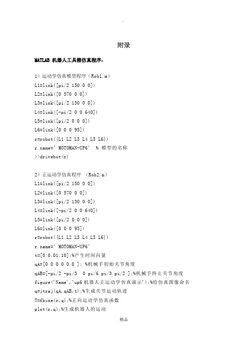
附录MATLAB 机器人工具箱仿真程序:1)运动学仿真模型程序(Rob1.m)L1=link([pi/2 150 0 0])L2=link([0 570 0 0])L3=link([pi/2 130 0 0])L4=link([-pi/2 0 0 640])L5=link([pi/2 0 0 0])L6=link([0 0 0 95])r=robot({L1 L2 L3 L4 L5 L6})=’MOTOMAN-UP6’ % 模型的名称>>drivebot(r)2)正运动学仿真程序(Rob2.m)L1=link([pi/2 150 0 0])L2=link([0 570 0 0])L3=link([pi/2 130 0 0])L4=link([-pi/2 0 0 640])L5=link([pi/2 0 0 0])L6=link([0 0 0 95])r=robot({L1 L2 L3 L4 L5 L6})=’MOTOMAN-UP6’t=[0:0.01:10];%产生时间向量qA=[0 0 0 0 0 0 ]; %机械手初始关节角度qAB=[-pi/2 -pi/3 0 pi/6 pi/3 pi/2 ];%机械手终止关节角度figure('Name','up6机器人正运动学仿真演示');%给仿真图像命名q=jtraj(qA,qAB,t);%生成关节运动轨迹T=fkine(r,q);%正向运动学仿真函数plot(r,q);%生成机器人的运动figure('Name','up6机器人末端位移图')subplot(3,1,1);plot(t, squeeze(T(1,4,:)));xlabel('Time (s)');ylabel('X (m)');subplot(3,1,2);plot(t, squeeze(T(2,4,:)));xlabel('Time (s)');ylabel('Y (m)');subplot(3,1,3);plot(t, squeeze(T(3,4,:)));xlabel('Time (s)');ylabel('Z (m)');x=squeeze(T(1,4,:));y=squeeze(T(2,4,:));z=squeeze(T(3,4,:));figure('Name','up6机器人末端轨迹图'); plot3(x,y,z);3)机器人各关节转动角度仿真程序:(Rob3.m)L1=link([pi/2 150 0 0 ])L2=link([0 570 0 0])L3=link([pi/2 130 0 0])L4=link([-pi/2 0 0 640])L5=link([pi/2 0 0 0 ])L6=link([0 0 0 95])r=robot({L1 L2 L3 L4 L5 L6})='motoman-up6't=[0:0.01:10];qA=[0 0 0 0 0 0 ];qAB=[ pi/6 pi/6 pi/6 pi/6 pi/6 pi/6]; q=jtraj(qA,qAB,t);Plot(r,q);subplot(6,1,1);plot(t,q(:,1));title('转动关节1');xlabel('时间/s');ylabel('角度/rad');subplot(6,1,2);plot(t,q(:,2));title('转动关节2');xlabel('时间/s');ylabel('角度/rad');subplot(6,1,3);plot(t,q(:,3));title('转动关节3');xlabel('时间/s');ylabel('角度/rad');subplot(6,1,4);plot(t,q(:,4));title('转动关节4');xlabel('时间/s');ylabel('角度/rad' );subplot(6,1,5);plot(t,q(:,5));title('转动关节5');xlabel('时间/s');ylabel('角度/rad');subplot(6,1,6);plot(t,q(:,6));title('转动关节6');xlabel('时间/s');ylabel('角度/rad');4)机器人各关节转动角速度仿真程序:(Rob4.m)t=[0:0.01:10];qA=[0 0 0 0 0 0 ];%机械手初始关节量qAB=[ 1.5709 -0.8902 -0.0481 -0.5178 1.0645 -1.0201]; [q,qd,qdd]=jtraj(qA,qAB,t);Plot(r,q);subplot(6,1,1);plot(t,qd(:,1));title('转动关节1');xlabel('时间/s');ylabel('rad/s');subplot(6,1,2);plot(t,qd(:,2));title('转动关节2');xlabel('时间/s');ylabel('rad/s');subplot(6,1,3);plot(t,qd(:,3));title('转动关节3');xlabel('时间/s');ylabel('rad/s');subplot(6,1,4);plot(t,qd(:,4));title('转动关节4');xlabel('时间/s');ylabel('rad/s' );subplot(6,1,5);plot(t,qd(:,5));title('转动关节5');xlabel('时间/s');ylabel('rad/s');subplot(6,1,6);plot(t,qd(:,6));title('转动关节6');xlabel('时间/s');ylabel('rad/s');5)机器人各关节转动角加速度仿真程序:(Rob5.m)t=[0:0.01:10];%产生时间向量qA=[0 0 0 0 0 0]qAB =[1.5709 -0.8902 -0.0481 -0.5178 1.0645 -1.0201]; [q,qd,qdd]=jtraj(qA,qAB,t);figure('name','up6机器人机械手各关节加速度曲线');subplot(6,1,1);plot(t,qdd(:,1));title('关节1');xlabel('时间 (s)');ylabel('加速度 (rad/s^2)');subplot(6,1,2);plot(t,qdd(:,2));title('关节2');xlabel('时间 (s)');ylabel('加速度 (rad/s^2)');subplot(6,1,3);plot(t,qdd(:,3));title('关节3');xlabel('时间 (s)');ylabel('加速度 (rad/s^2)')subplot(6,1,4);plot(t,qdd(:,4));title('关节4');xlabel('时间 (s)');ylabel('加速度 (rad/s^2)')subplot(6,1,5);plot(t,qdd(:,5));title('关节5');xlabel('时间 (s)');ylabel('加速度 (rad/s^2)')subplot(6,1,6);plot(t,qdd(:,6));title('关节6');xlabel('时间 (s)');ylabel('加速度 (rad/s^2)')如有侵权请联系告知删除,感谢你们的配合!。
如何在MATLAB中进行移动机器人控制
如何在MATLAB中进行移动机器人控制在现代机器人技术领域中,移动机器人控制是一个非常重要的研究方向。
移动机器人是指能够在环境中自主移动和执行任务的机器人。
而利用MATLAB软件进行移动机器人控制不仅可以帮助我们更好地理解机器人的运动规律,还可以实现对机器人的精确控制。
本文将从控制理论和MATLAB编程的角度,探讨如何在MATLAB中进行移动机器人控制。
## 一、移动机器人控制的基本理论在移动机器人控制中,我们需要考虑的一个重要问题是机器人的运动学和动力学。
机器人的运动学研究机器人在空间中的运动和姿态,而动力学则研究机器人的运动和力学关系。
了解机器人的运动学和动力学对于实现精确的控制至关重要。
在移动机器人控制中,我们通常会使用轨迹规划算法来生成机器人的运动轨迹。
轨迹规划算法可以根据机器人的起始位置、目标位置和环境约束,生成一条机器人运动轨迹。
常用的轨迹规划算法包括最速轨迹、最短路径和避障路径等。
另一个重要的控制理论是PID控制器。
PID控制器是一种经典的反馈控制器,可以根据机器人当前状态和目标状态之间的偏差来调整控制指令,从而实现对机器人的控制。
PID控制器在移动机器人控制中得到了广泛应用,因为它简单易懂、调节性能好。
## 二、MATLAB在移动机器人控制中的应用MATLAB是一种流行的数值计算和科学编程环境,被广泛应用于机器人控制领域。
MATLAB提供了很多工具箱和函数,可以用于在MATLAB环境中进行移动机器人控制。
首先,我们可以使用MATLAB中的机器人工具箱进行机器人模型的建立和仿真。
机器人工具箱提供了一系列函数和方法,可以帮助我们建立机器人模型,并对机器人进行仿真。
通过仿真实验,我们可以预测机器人的运动和行为,并进行控制算法的验证和优化。
其次,MATLAB中的机器人工具箱还提供了一些常用的轨迹规划算法,如最速轨迹和最短路径规划算法。
我们可以利用这些算法生成机器人的运动轨迹,并进行仿真和控制实验。
基于Coppeliasim与MATLAB的机器人建模与运动仿真

绕 #$ 轴旋转 $5$ "使得 %$ 和 %$5$ 互相平行"因为 !$ 和 !!5都是垂直于 #$ 轴"因此绕 #$ 旋转 $5$ 使它们平行' 并 且共面( % 绕 #$ 轴平移 "$5$ "使得 %$ 和 %$5$ 共线"因为 %$ 和 %$5$ 都是平行并且垂直于 #$ 轴"沿着 #$ 移动则可以使 它们重叠在一起% 绕 %$ 轴平移 "$5$ "使得 %$ 和 %$5$ 的原 点坐标相同% #$ 围绕 %$5$ 旋转 !$5$ "使得 #$ 轴和 #$5$ 轴处 在同一条线上"使得变换前后的坐标系完全重合% 通过上 述变换步骤"得到准确的坐标系变换,$$- %
',O7< J4P0?490?< 02>79R0?S7E@059?01-<D978-/75<456L5D9=9;9702M;90849=05@/=57D7M.4E78< 02-.=75.7D J=405=56-/75<456!&&%%&(
$,L5D9=9;9702T0P09=.D 45EL59711=6759345;24.9;?=56L550H49=05@/=57D7M.4E78< 02-.=75.7D J=405=56-/75<456&&%&(+
,HE$
h
E/-$
% %
lE/-$ ,HE$ ,HE$ ,HE$
E/-$ %
E/-$ E/-$ l,HE$ E/-$
,HE$ %
!$ '()$ !$ E/-$
MATLAB-SimMechanics机构动态仿真
个方向转动)、Bushing(三个方向移动,三个方
向转动)、Custom Joint(自定义铰)、
Cylindrical(柱面铰)、Gimbal(万向铰,旋转
三个角度)、In-plane(平面内移动)、Planar
(平面铰)、Prismatic(单自由运动铰)、
Revolute(单自由转动铰)、Screw(螺旋铰)、
扑结构,但至少有一个构件是Ground模块,而且
有一个环境设置模块直接与其相连。
一个构件可能不止两个铰(Joint),即可以
产生分支。但是一个较只能连接两个构件。
(3)配置Body模块:双击模块,打开参数对话
框,配置质量属性(质量和惯性矩),然后确定
Body模块和Ground模块与整体坐标系或其他坐标
• 1.双击Disassembled Joints,弹出如图模块组, 其中模块是分解后的铰,不同于Joints中对应的 铰,它们有不同的基准点。
2021/7/1
14
• 2.双击Massless Connectors,弹出如图模块组, 其中模块是Joint中对应的铰的组合。
2021/7/1
15
4.2.6 传Βιβλιοθήκη 器与激励器模块组(Sensors&Actuators)
• 双击模块,弹出图示模块组。该模块组中的模块 用来和普通的Simulink模块进行数据交换。
2021/7/1
16
• Body Actuator:通过广义力或力矩来驱动刚体。 • Body Sensor:刚体检测模块。 • Constraint&Drivr Sensor:检测一对受约束刚体
间的力或力矩。 • Driver Actuator:对一对互相约束的刚体施加相
机器人控制matlab版
机器人控制matlab版机器人控制是指通过编程和算法控制机器人的运动和行为。
MATLAB作为一种强大的科学计算软件和工具,可以广泛应用于机器人控制领域。
本文将介绍机器人控制的MATLAB版,包括机器人模型、控制算法和实例应用等。
一、机器人模型在机器人控制之前,需要先建立机器人模型。
机器人模型是机器人的数学表达,用于描述机器人的结构和动力学特性。
常见的机器人模型包括末端执行器模型、刚体模型和关节模型等。
在MATLAB中,可以使用Robotics System Toolbox来建立机器人模型。
该工具箱提供了一系列函数和类,可以方便地创建机器人模型,并进行正向和逆向运动学计算。
二、控制算法机器人控制的核心是控制算法。
控制算法可以分为运动控制和轨迹规划两个方面。
1. 运动控制运动控制是控制机器人执行特定动作的算法。
常见的运动控制算法包括PID控制、反馈线性化控制和自适应控制等。
在MATLAB中,可以使用Control System Toolbox来设计和实现运动控制算法。
该工具箱提供了丰富的函数和方法,可以进行控制器设计、系统建模和仿真等操作。
2. 轨迹规划轨迹规划是控制机器人在给定时间内从初始位置到达目标位置的算法。
常见的轨迹规划算法包括直线插补、三次样条插补和最短路径规划等。
在MATLAB中,可以使用Robotics System Toolbox中的轨迹生成器函数来进行轨迹规划。
该工具箱提供了一系列的插补函数,可以方便地生成平滑的运动轨迹。
三、实例应用机器人控制的应用非常广泛,包括工业制造、医疗卫生和服务机器人等领域。
以工业制造为例,机器人控制可以实现自动化生产线的操作和控制。
通过MATLAB中的机器人控制工具箱,可以对机器人进行建模、控制和仿真,实现自动化生产线的规划和优化。
此外,机器人控制还可以应用于医疗卫生领域。
例如,通过MATLAB编写的机器人控制程序,可以控制外科手术机器人进行精确的手术操作,提高手术的安全性和准确性。
机器人系统常用仿真软件介绍

1 主要介绍以下七种仿真平台(侧重移动机器人仿真而非机械臂等工业机器人仿真):1.1 USARSi m-Unifie d System for Automa tionand RobotSimula tionUSARSi m是一个基于虚拟竞技场引擎设计高保真多机器人环境仿真平台。
主要针对地面机器人,可以被用于研究和教学,除此之外,USARSi m是Rob oCup救援虚拟机器人竞赛和虚拟制造自动化竞赛的基础平台。
使用开放动力学引擎ODE(Open Dynami cs Engine),支持三维的渲染和物理模拟,较高可配置性和可扩展性,与Player兼容,采用分层控制系统,开放接口结构模拟功能和工具框架模块。
机器人控制可以通过虚拟脚本编程或网络连接使用UDP协议实现。
被广泛应用于机器人仿真、训练军队新兵、消防及搜寻和营救任务的研究。
机器人和环境可以通过第三方软件进行生成。
软件遵循免费GPL条款,多平台支持可以安装并运行在Linux、Window s和Mac OS操作系统上。
1.2 SimbadSimbad是基于Ja va3D的用于科研和教育目的多机器人仿真平台。
主要专注于研究人员和编程人员热衷的多机器人系统中人工智能、机器学习和更多通用的人工智能算法一些简单的基本问题。
它拥有可编程机器人控制器,可定制环境和自定义配置传感器模块等功能,采用3D虚拟传感技术,支持单或多机器人仿真,提供神经网络和进化算法等工具箱。
软件开发容易,开源,基于GNU协议,不支持物理计算,可以运行在任何支持包含Java3D库的Ja va客户端系统上。
1.3 WebotsWebots是一个具备建模、编程和仿真移动机器人开发平台,主要用于地面机器人仿真。
MATLAB机器人仿真程序
MATLAB机器人仿真程序哎呀,说起 MATLAB 机器人仿真程序,这可真是个有趣又充满挑战的领域!我还记得有一次,我带着一群学生尝试做一个简单的机器人行走仿真。
那时候,大家都兴奋极了,眼睛里闪着好奇的光。
我们先从最基础的开始,了解 MATLAB 这个工具的各种函数和命令。
就像是给机器人准备好各种“零部件”,让它能顺利动起来。
比如说,我们要设定机器人的初始位置和姿态,这就好像是告诉机器人“嘿,你从这里出发,站好啦!”然后,再通过编程来控制它的运动轨迹。
有的同学想让机器人走直线,有的同学想让它拐个弯,还有的同学想让它走个复杂的曲线。
在这个过程中,可遇到了不少问题呢。
有个同学不小心把坐标设置错了,结果机器人“嗖”地一下跑到了不知道哪里去,大家哄堂大笑。
还有个同学在计算速度和加速度的时候出了差错,机器人的动作变得奇奇怪怪的,像是在跳“抽筋舞”。
不过,大家并没有气馁,而是一起努力找错误,修改代码。
终于,当我们看到那个小小的机器人按照我们设想的轨迹稳稳地行走时,那种成就感简直无法形容。
回到 MATLAB 机器人仿真程序本身,它其实就像是一个神奇的魔法盒子。
通过输入不同的指令和参数,我们可以创造出各种各样的机器人运动场景。
比如说,我们可以模拟机器人在不同地形上的行走,像是平坦的地面、崎岖的山路或者是湿滑的冰面。
这时候,我们就要考虑摩擦力、重力等各种因素对机器人运动的影响。
想象一下,机器人在冰面上小心翼翼地走着,生怕滑倒,是不是很有趣?而且,MATLAB 机器人仿真程序还能帮助我们优化机器人的设计。
比如说,如果我们发现机器人在某个动作上消耗了太多的能量,或者动作不够灵活,我们就可以通过调整程序中的参数来改进。
这就像是给机器人做了一次“整形手术”,让它变得更完美。
另外,我们还可以用它来进行多机器人的协同仿真。
想象一下,一群机器人在一起工作,有的负责搬运东西,有的负责巡逻,它们之间需要相互配合,避免碰撞。
这就需要我们精心设计它们的通信和协调机制,让它们像一支训练有素的团队一样高效工作。
机器人matlab仿真课程设计
机器人matlab仿真课程设计一、教学目标本课程的教学目标是使学生掌握机器人Matlab仿真基本原理和方法,能够运用Matlab进行简单的机器人系统仿真。
具体分解为以下三个目标:1.知识目标:学生需要了解机器人Matlab仿真的基本原理,掌握Matlab在机器人领域中的应用方法。
2.技能目标:学生能够熟练使用Matlab进行机器人系统的仿真,包括建立仿真模型、设置仿真参数、运行仿真实验等。
3.情感态度价值观目标:通过课程学习,培养学生对机器人技术的兴趣和热情,提高学生解决实际问题的能力,培养学生的创新精神和团队合作意识。
二、教学内容教学内容主要包括以下几个部分:1.Matlab基础知识:介绍Matlab的基本功能和操作,包括数据处理、图形绘制、编程等。
2.机器人数学模型:介绍机器人的运动学、动力学模型,以及传感器和执行器的数学模型。
3.机器人仿真原理:讲解机器人仿真的一般方法和步骤,包括建立仿真模型、设置仿真参数、运行仿真实验等。
4.机器人控制系统仿真:介绍机器人控制系统的结构和原理,以及如何使用Matlab进行控制系统仿真。
5.机器人路径规划仿真:讲解机器人在复杂环境中的路径规划方法,以及如何使用Matlab进行路径规划仿真。
三、教学方法为了达到上述教学目标,我们将采用以下教学方法:1.讲授法:通过讲解和演示,使学生了解机器人Matlab仿真的基本原理和方法。
2.案例分析法:通过分析实际案例,使学生掌握Matlab在机器人领域中的应用。
3.实验法:让学生亲自动手进行机器人仿真实验,巩固所学知识,提高实际操作能力。
4.小组讨论法:鼓励学生分组讨论,培养学生的团队合作意识和解决问题的能力。
四、教学资源为了支持教学内容的实施,我们将准备以下教学资源:1.教材:《机器人Matlab仿真教程》。
2.参考书:相关领域的研究论文和书籍。
3.多媒体资料:教学PPT、视频教程等。
4.实验设备:计算机、Matlab软件、机器人仿真实验平台。
SCARA机器人MATLAB仿真实验报告
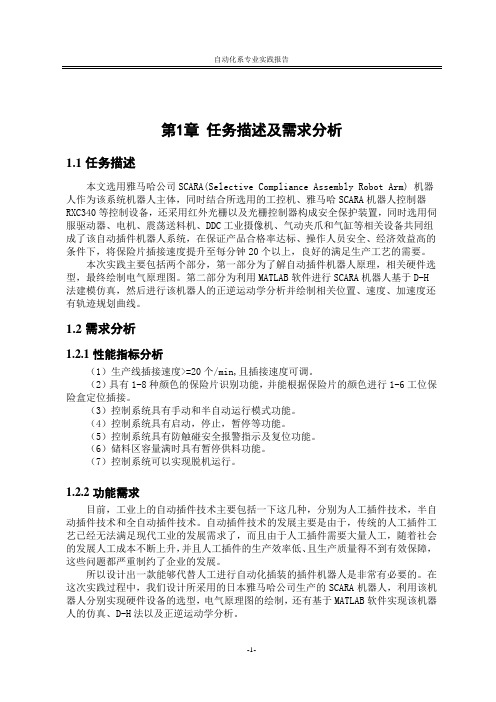
第1章任务描述及需求分析1.1任务描述本文选用雅马哈公司SCARA(Selective Compliance Assembly Robot Arm) 机器人作为该系统机器人主体,同时结合所选用的工控机、雅马哈SCARA机器人控制器RXC340等控制设备,还采用红外光栅以及光栅控制器构成安全保护装置,同时选用伺服驱动器、电机、震荡送料机、DDC工业摄像机、气动夹爪和气缸等相关设备共同组成了该自动插件机器人系统,在保证产品合格率达标、操作人员安全、经济效益高的条件下,将保险片插接速度提升至每分钟20个以上,良好的满足生产工艺的需要。
本次实践主要包括两个部分,第一部分为了解自动插件机器人原理,相关硬件选型,最终绘制电气原理图。
第二部分为利用MATLAB软件进行SCARA机器人基于D-H 法建模仿真,然后进行该机器人的正逆运动学分析并绘制相关位置、速度、加速度还有轨迹规划曲线。
1.2需求分析1.2.1性能指标分析(1)生产线插接速度>=20个/min,且插接速度可调。
(2)具有1-8种颜色的保险片识别功能,并能根据保险片的颜色进行1-6工位保险盒定位插接。
(3)控制系统具有手动和半自动运行模式功能。
(4)控制系统具有启动,停止,暂停等功能。
(5)控制系统具有防触碰安全报警指示及复位功能。
(6)储料区容量满时具有暂停供料功能。
(7)控制系统可以实现脱机运行。
1.2.2功能需求目前,工业上的自动插件技术主要包括一下这几种,分别为人工插件技术,半自动插件技术和全自动插件技术。
自动插件技术的发展主要是由于,传统的人工插件工艺已经无法满足现代工业的发展需求了,而且由于人工插件需要大量人工,随着社会的发展人工成本不断上升,并且人工插件的生产效率低、且生产质量得不到有效保障,这些问题都严重制约了企业的发展。
所以设计出一款能够代替人工进行自动化插装的插件机器人是非常有必要的。
在这次实践过程中,我们设计所采用的日本雅马哈公司生产的SCARA机器人,利用该机器人分别实现硬件设备的选型,电气原理图的绘制,还有基于MATLAB软件实现该机器人的仿真、D-H法以及正逆运动学分析。
advisor使用介绍
第6章 ADVISOR模拟计算软件的详细分析ADVISOR(Advanced Vehicle Simulator),是由美国国家可再生能源实验室开发的仿真软件,可以仿真纯电动汽车、串联式或者并联式混合动力电动汽车以及传统的内燃机汽车。
ADVISOR是在Matlab/Simulink下开发而成,它的图形用户界面可以使用户很容易地改变汽车模型的参数,而不要修改Simulink代码。
它具有各种类型的零部件模型以及很大的灵活性,可以仿真任何类型的HEV 和内燃机汽车。
ADVISOR可以使用用户自己订制的循环工矿以及各种标准工况,它的仿真结果包括燃油经济性、排放、加速性能等各种所需要的数据。
6.1 Matlab/Simulink 介绍Simmlink是一个用来对动态系统进行建模、仿真和分析的软件包。
它支持线性和非线性系统,连续和离散时间模型,或者是两者的混合。
系统还可以是多采样率的,比如系统的不同部分拥有不同的采样率,另外,Simulink还提供一套图形动画的处理方法,使用户可以方便地观察到仿真的整个过程。
Simulink没有单独的语言,但它提供了S函数规则。
所谓的S函数可以是一个M 文件、FORTRAN程序、C或C++语言程序等,通过特殊的语法规则使之能够被Simulink模型或模块调用。
S(以后有关章节详细讲解)函数使Simulink更加充实、完备,具有更强的处理能力。
同MATLAB一样,Simulink也不是封闭的,它允许用户可以很方便地定制自己的模块和模块库。
同时Simulink也同样有比较完整的帮助系统,使用户可以随时找到对应模块的说明,便于应用。
目前,随着软件的不断升级换代,Simulink在软硬件的接口方面有了长足的进步,使用Simulink已经可以很方便地进行实时的信号控制和处理、信息通信以及DSP的处理。
世界上许多知名大公司已经使用Simulink作为他们产品设计和开发的强有力工具,ADVISOR 就是在这种条件下产生的。
MICROAUTOBOX技术资料说明
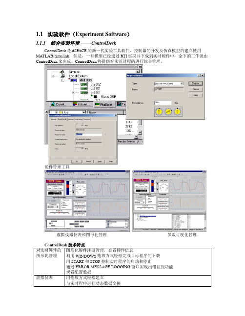
1.1实验软件(Experiment Software)1.1.1综合实验环境—— ControlDeskControlDesk是dSPACE的新一代实验工具软件。
控制器的开发及仿真模型的建立使用MATLAB/simulink,但是,一旦模型已经通过RTI实现并下载到实时硬件中,余下的工作就由ControlDesk来完成。
ControlDesk将提供对实验过程的进行综合管理。
硬件管理工具虚拟仪器仪表和图形化管理参数可视化管理ControlDesk 技术特点对实时硬件的图形化管理图形化硬件注册管理,查看硬件信息利用WINDOWS拖放方式轻松完成目标程序的下载用START和STOP控制实时程序的启动和停止通过ERROR MESSAGE LOGGING窗口实现出错监视功能观看配置数据虚拟仪表用拖放方式轻松建立与实时程序进行动态数据交换Pidr跟踪实时曲线在线调参记录实时数据(可记录在文件中)实时数据回放提供各种专业虚拟仪表库(汽车库等)变量的可视化管理以图形方式访问RTI生成的变量文件通过拖放操作在变量和虚拟仪表之间建立联系除访问一般变量外,还可访问诸如采样时间、中断优先级、程序执行时间等其它与实时操作相关的变量参数的可视化管理可根据实时变量树生成参数文件通过参数文件对实时试验进行批参数修改通过多个参数文件的顺序调入,研究不同参数组对实时试验的影响实验过程自动化提供到ControlDesk所有组成部分的编程接口对耗时及需重复进行的试验过程可以实现自动化,如:参数研究利用Macro Recorder记录ControlDesk的操作利用面向对象的功能强大的算法语言编制自动试验算法提供到MA TLAB接口,实现与MATLAB的数据交换另外,在与多处理器系统配合使用时,需要ControlDesk Multiprocessor Extenssion。
1.1.2故障仿真—— ControlDesk(Failure Simulation)•对标准ControlDesk功能的扩展•在中型或大型dSPACE模拟器中远程控制故障注入单元•通过故障仿真浏览器可访问所有故障仿真部件•在故障模式窗口中实现管脚错误定义•可导入ECU管脚描述文件ControlDesk的故障仿真功能使得操作dSPACE模拟器的故障注入单元变得非常便利。
abms的名词解释

abms的名词解释ABMS(Agent-Based Modelling and Simulation)是一种基于智能体的建模和仿真方法。
它是一种模拟社会或自然系统中个体行为和交互的技术。
ABMS的成功应用可以追溯到二十世纪七八十年代的计算机科学和人工智能领域,随着计算能力的提高和软件工具的发展,ABMS在近年来得到了广泛应用和研究。
在传统的建模和仿真方法中,通常通过数学方程式来表示和描述系统的行为和动态。
然而,这种方法往往忽略了系统中个体之间的相互作用和反馈机制,从而限制了对复杂系统的理解和预测能力。
ABMS正是为了解决这一问题而产生的一种新型建模和仿真方法。
ABMS的核心思想是将系统看作由个体智能体组成的集合,每个智能体都具有自己的特征、状态和行为规则。
这些智能体可以通过感知环境、与其他智能体进行交互以及根据预定的规则进行决策来模拟真实世界。
ABMS能够模拟多种复杂系统,如城市交通、社会网络、生态系统、金融市场等。
通过对智能体的建模,ABMS可以更好地理解系统中个体的行为模式、相互作用和决策过程,从而推断整个系统的行为和演变。
ABMS的应用领域非常广泛。
在城市规划中,ABMS可以用于模拟交通流量,优化交通信号控制,减少交通拥堵;在社会科学中,ABMS可以用于研究社会网络、群体行为和意见传播等问题;在生物学和生态学领域,ABMS可以用于模拟生物进化、种群动态和生态系统的演变。
与传统建模方法相比,ABMS具有以下几个优点:1. 能够模拟复杂系统的多样性和异质性。
由于ABMS关注个体智能体的行为规则和决策过程,它可以更好地模拟和理解现实世界中的多样性和异质性。
2. 能够模拟系统的动态演变和反馈机制。
ABMS通过模拟个体之间的相互作用和决策过程,可以捕捉系统演变的动态性以及反馈机制的作用。
3. 能够进行实验和预测。
ABMS可以对系统进行实验和敏感性分析,通过调整智能体的行为规则和参数,并观察系统的响应来推测系统的未来行为。
多机器人编队控制matlab仿真代码
多机器人编队控制matlab仿真代码1.引言1.1 概述在引言部分的概述中,我们将重点介绍多机器人编队控制的基本概念和研究背景。
随着技术的不断发展,机器人在各个领域中得到了广泛的应用,尤其是在无人系统和自主导航领域。
多机器人编队控制是指通过在多个机器人之间建立合作关系和协同工作,实现一定的任务目标。
在这种编队控制中,多个机器人之间需要交换信息、协调动作,并按照一定的规则进行排列或者协同工作。
在过去的几十年中,多机器人编队控制已经成为机器人领域的一个热点研究方向。
它在军事、灾害救援、工业生产等领域中发挥重要的作用。
多机器人编队控制可以提高任务的执行效率,增强系统的鲁棒性和可靠性,并且可以应对一些单个机器人无法完成的大规模任务。
为了实现多机器人编队控制,研究人员提出了各种不同的控制策略和算法。
这些控制策略可以分为集中式和分布式两种方式。
集中式控制是指由一个中心节点来控制整个编队的行为,而分布式控制则是指每个机器人根据本地信息和与邻近机器人的通信,来决定自己的行为。
通过多机器人编队控制,可以实现机器人之间的任务分工和协同工作,提高整个系统的性能和效率。
此外,多机器人编队控制还涉及到一些重要的问题,如编队形成、路径规划、障碍物避障、通信协议等。
本文将从多机器人编队控制的概述开始,介绍其重要性,并对未来的研究方向进行展望。
通过对多机器人编队控制的研究,我们可以进一步推动机器人技术的发展,并为解决各种实际问题提供更加高效和可靠的解决方案。
1.2 文章结构文章结构部分的内容可以这样编写:本文将按照以下结构进行介绍和讨论多机器人编队控制的相关内容:1. 引言:首先概述了多机器人编队控制的概念和背景,以及本文的目的。
2. 正文:分为两个部分进行介绍。
2.1 多机器人编队控制概述:详细解释了什么是多机器人编队控制,包括其定义、目标和应用领域。
同时,介绍了多机器人编队控制的研究现状和发展趋势。
2.2 多机器人编队控制的重要性:着重论述了多机器人编队控制的重要性和优势。
基于MATLAB Robotics Toolbox的机器人学仿真实验教学
基于MATLAB Robotics Toolbox的机器人学仿真实验教学摘要:简要介绍MATLAB Robotics Toolbox在机器人学仿真实验教学中的基本应用,具体内容包括齐次坐标变换、机器人对象构建、机器人运动学求解以及轨迹规划等。
该工具箱可以对机器人进行图形仿真,并能分析真实机器人控制时的实验数据结果,因此非常适宜于机器人学的教学和研究。
关键词:机器人学;仿真实验教学;MATLAB;Robotics Toolbox机器人学是一门高度交叉的前沿学科方向,也是自动化和机电工程等相关专业的一门重要专业基础课。
在机器人学的教学和培训中,实验内容一直是授课的重点和难点。
实物机器人通常是比较昂贵的设备,这就决定了在实验教学中不可能运用许多实际的机器人来作为教学和培训的试验设备。
由于操作不方便、体积庞大等原因,往往也限制了实物机器人在课堂授课时的应用。
此外,由于计算量、空间结构等问题,当前大多数机器人教材只能以简单的两连杆机械手为例进行讲解,而对于更加实际的6连杆机械手通常无法讲解得很清楚。
因此,各式各样的机器人仿真系统应运而生。
经过反复的比较,我们选择了MATLAB Robotics Toolbox [1]来进行机器人学的仿真实验教学。
MATLAB Robotics Toolbox是由澳大利亚科学家Peter Corke开发和维护的一套基于MATLAB的机器人学工具箱,当前最新版本为第8版,可在该工具箱的主页上免费下载(/robot/)。
Robotics Toolbox提供了机器人学研究中的许多重要功能函数,包括机器人运动学、动力学、轨迹规划等。
该工具箱可以对机器人进行图形仿真,并能分析真实机器人控制时的实验数据结果,因此非常适宜于机器人学的教学和研究。
本文简要介绍了Robotics Toolbox在机器人学仿真实验教学中的一些应用,具体内容包括齐次坐标变换、机器人对象构建、机器人运动学求解以及轨迹规划等。
软件产品系统仿真system simulator
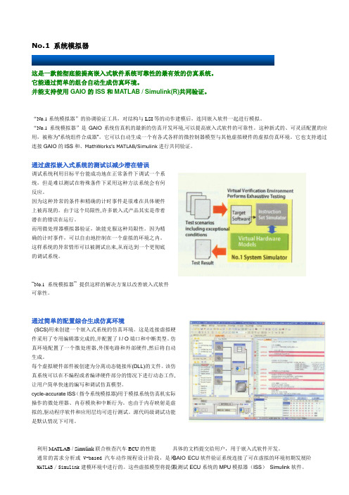
No.1 系统模拟器这是一款能彻底能提高嵌入式软件系统可靠性的最有效的仿真系统。
它能通过简单的组合自动生成仿真环境。
并能支持使用GAIO 的ISS 和MATLAB / Simulink(R)共同验证。
“No.1系统模拟器”的协调验证工具,对结构与LSI 等的动作建模后,连同嵌入软件一起进行模拟。
“No.1系统模拟器”是GAIO 系统仿真机的最新的仿真开发环境,可以提高嵌入式软件的可靠性。
这种新式的、可灵活配置的应用,被称为“系统组件合成器”。
它可以自动生成一个有各式各样的微控制器模型与其他虚拟硬件的虚拟仿真环境。
它也支持通过连接GAIO 的ISS 和、MathWorks’s MATLAB/Simulink 进行共同验证。
通过虚拟嵌入式系统的测试以减少潜在错误调试系统利用目标平台能成功地在正常条件下调试一个系统,但是难以测试在特殊条件下采用这种方法系统会有何反应。
因为这种异常的条件和精确的计时事件是很难在具体硬件上被再现的。
由于这个局限性,许多嵌入式产品其实是带着潜在的错误在运行。
而用微处理器模拟器验证,缺能克服这种局限性。
因为精确的计时事件,可以自由地控制在一个虚拟的环境之内。
这样系统的异常情形可以被测试出来,从而达到一个更彻底的调试系统。
“No.1系统模拟器” 提供这样的解决方案以改善嵌入式软件可靠性。
通过简单的配置综合生成仿真环境(SCS)用来创建一个嵌入式系统的仿真环境。
这是连接虚拟硬件采用了专用编辑器完成的,并配置了I / O 端口和中断类型。
仿真环境配置了一个微处理器,外围电路和外部硬件,然后将自动生成。
每个虚拟硬件部件被创建为分离动态链接库(DLL)的文件。
该仿真系统可以在不编程或者编译硬件部分的情况下进行动态工作, 让用户简单快速的编写和调试仿真模型。
cycle-accurate ISS (指令系统模拟器)用于模拟系统仿真机实际操作的微处理器、内存模块和中断行为。
也由于内存映射是虚拟的,驱动程序软件和应用层均可进行测试。
基于Coppeliasim与MATLAB的机器人建模与运动仿真
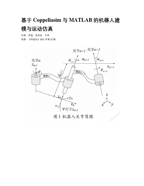
基于Coppeliasim与MATLAB的机器人建模与运动仿真作者:李杨张华良王军来源:《科技风》2021年第32期摘要:针对目前机器人模型构建烦琐,仿真过程复杂的问题,提出了基于Coppeliasim与MATLAB相结合实现对所研究机器人的建模与运动仿真。
首先使用3D建模软件SolidWorks 将模型导出,然后采用D-H参数建模法进行分析,得出机器人运动学模型表达式。
最后使用LuaSocket通信方式实现机器人与MATLAB中控制程序之间的通信连接。
目的是实现机器人复杂的运动学建模与运动仿真。
该方法研究了机器人关节运动和控制程序,分析了二者联合仿真的实用性。
以络石XB7机器人为代表,叙述机器人的3D模型仿真技术。
仿真结果表明机器人能够准确按照控制程序进行运动,验证本仿真方法的真实有效性。
关键词:机器人;Coppeliasim仿真;LuaSocket;D-H模型中图分类号:TP-242 文献标识码:A随着机器人建模与仿真在工业技术领域占有比重越来越大,在机器人设计与制造过程中,能够提前解决机器人运行中出现的问题,并避免在实操中呈现的各种安全隐患问题也变得尤为重要。
根据不同的仿真目标选择仿真工具成为开发机器人的关键。
L Pitonakova等人提出了V-REP,Gazebo和ARGOS机器人模拟器的功能和性能比较。
2019年11月,V-REP被重新命名为Coppeliasim,Coppeliasim在V-REP的基础上重写计算例程、碰撞处理检测、最短路径计算、超频树、近似传感器模拟以及点云方面,显著提高了运行速度。
但Coppeliasim仿真运动过程只能根据脚本执行,可操作性能差。
祁若龙等人指出MATLAB在机器人仿真领域应用广泛,但是MATLAB仿真在三维空间构型能力差,不能完整清晰的各个连杆与末端问的姿态。
本文针对以上的不足,提出了结合Coppeliasim与MATLAB通过LuaSocket通信使用控制器对机械臂控制,并得到机器人运动的关节角以及运动轨迹曲线。
基于MATLAB软件的四足步行机器人的运动学仿真_李赫
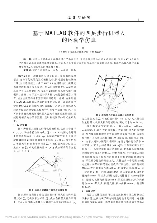
图 1 机 器人 腿 部 连杆 简 化 后 的模 型 图
图 2 所示为当腿 2 作为摆动腿时机器人的结构示意 图, 其 中 ∑ 0 代 表参 考 坐 标 系 , ∑ C 代 表 在机 器 人 机 身 平 面
c 上、 原 点 c 与 机 器 人 机 体几 何 对 称 中 心 重 合 的 坐 标 系 , p Ai
b T 园 - 糟责 月蚤 p Ai=R ( 责 粤蚤 原 园责 糟) 糟
我 们可 以 得到
b
(圆)
[bxAi p Ai= [园xAi p Ai= [园xc p c=
0
b
yAi yA i
0
b
T z Ai]
(3) (4) (5)
-1 c T 0 c c
与
园 0 0 T z Ai]
和
园
yc
T z c]
的关系, 它们都是关于时间 t 的函数。其中, 公式 (2) 中 Rc 代表坐标系∑C 相对于坐标系∑0 的方向矩阵, R =R , p ,代表 坐标系∑C 原点在 c 坐标系∑0 中的位置矢量。 再由单腿的逆运 动学公式
李 赫
(吉 林 电 子 信 息 职 业 技 术 学 院 , 吉 林 132021)
摘
要: 按照一定的要求对机器人进行了参数 设定, 通 过分 析 机器 人 的逆 运 动学 问 题, 运 用 MATLAB 软 件
中的编写函数功能进行运动学仿真, 得出各个关节在仿真时间内 光 滑的运动 轨迹曲线, 验证了机器人连 杆 参数 的 合理性 , 从而 能 够达到预 定的 目标。 关键词: 四足 步 行机器人 步态 运动学 仿真
扇 设 设 设 设 设 设 设 设 设 设 设 设 缮 设 设 设 设 设 设 设 设 设 设 设 设 墒
- 1、下载文档前请自行甄别文档内容的完整性,平台不提供额外的编辑、内容补充、找答案等附加服务。
- 2、"仅部分预览"的文档,不可在线预览部分如存在完整性等问题,可反馈申请退款(可完整预览的文档不适用该条件!)。
- 3、如文档侵犯您的权益,请联系客服反馈,我们会尽快为您处理(人工客服工作时间:9:00-18:30)。
A Matlab-based Simulator for Autonomous Mobile RobotsAbstractMatlab is a powerful software development tool and can dramatically reduce the programming workload during the period of algorithm development and theory research. Unfortunately, most of commercial robot simulators do not support Matlab. This paper presents a Matlab-based simulator for algorithm development of 2D indoor robot navigation. It provides a simple user interface for constructing robot models and indoor environment models, including visual observations for the algorithms to be tested. Experimental results are presented to show the feasibility and performance of the proposed simulator.Keywords: Mobile robot, Navigation, Simulator, Matlab1. IntroductionNavigation is the essential ability that a mobile robot. During the development of new navigation algorithms, it is necessary to test them in simulated robots and environments before the testing on real robots and the real world. This is because (i) the prices of robots are expansive; (ii) the untested algorithm may damage the robot during the experiment; (iii) difficulties on the construction and alternation of system models under noise background; (iv) the transient state is difficult to track precisely; and (v) the measurements to the external beacons are hidden during the experiment, but this information is often helpful for debugging and updating the algorithms.The software simulator could be a good solution for these problems. A good simulator could provide many different environments to help the researchers to find out problems in their algorithms in different kinds of mobile robots. In order to solve the problems listed above, this simulator is supposed to be able to monitor system states closely. It also should have flexible and friendly users’ interface to develop all kinds of algorithms.Up to now, many commercial simulators with good performance have been developed. For instance, MOBOTSIM is a 2D simulator for windows, which provides a graphic interface to build environments [1]. But it only supports limited robot models (differential driven robots with distance sensors only), and is unable to deal with on visual based algorithms. Bugworks is a very simple simulator providing drag-and-place interface [2]; but it provides very primitive functions and is more like a demonstration rather than a simulator. Some other robot simulators, such as Ropsim [3], ThreeDimSim [5], and RPG Kinematix [6], are not specially designed for the development of autonomous navigation algorithms of mobile robots and have very limited functions.Among all the commercial simulators, Webot from Cyberbotics [4] and MRS from Microsoft are powerful and better performed simulators for mobile robot navigation. Both simulators, i.e. Webots and MRS, provide powerful interfaces to build mobile robots and environments, excellent 3-D display, accurate performance simulation, and programming languages for robot control. Perhaps due to the powerful functions, they are difficult to use for a new user. For instance, it is quite a boring job to build an environment for visual utilities, which involves shapes building, materials selection, and illumination design. Moreover, some robot development kits have built-in simulator for some special kinds of robots. Aria from Activmedia has a 2-D indoor simulator for Pioneer mobile robots [8]. The simulator adopts feasible text files to configure the environment, but only support limited robot models.However, the majority of commercial simulators are not currently supporting On the other hand, Matlabprogramming that provides a good support in matrix computing, image processing, fuzzy logic, neural network, etc., and can dramatically reduce the coding time in the research stage of new navigation algorithms. For example, a matrix inverse operation may needs a function which has hundreds of lines; but there is a simple command in Matlab. To use Matlab in this stage can avoid time-wasting on regenerating existed algorithms repeatedly and focus on the new theory and algorithm development.This paper presents a Matlab-based simulator that is fully compatible with Matlab codes, and makes it possible for robotics researchers to debug their code and do experiments conveniently at the first stage of their research. The algorithms development is based on Matlab subroutines with appointed parameter variables, which are stored in a file to be accessed by the simulator. Using this simulator, we can build the environment, select parameters, build subroutines and display outputs on the screen. Data are recorded during the whole procedure; some basic analyses are also performed.The rest of the paper is organized as follows. The software structure of the proposed simulator is explained in Section II. Section III describes the user interface of the proposed simulator. Some experimental results are given in Section IV to show the system performance. Finally, Section V presents a brief conclusion and potential future work.2. Software architectureTo make algorithm design and debugging easier, our Matlab based simulator has been designed to have the following functions:●Easy environment model-building; including walls, obstacles, beacons and visual scenes;●Robot model building, including the driving and control system and noise level.●Observation model setting; the simulator calculates the image frame that the robot can see, according tothe precise robot pose, the parameters of camera, and the environment.●Bumping reaction simulation. If the robot touches “walls”, the simula tor can stop the robot even when itis commanded to move forward by other modules. This function prevents the robot passing through the “wall” like a ghost, and makes the simulation running like the experiment on real robots.●Real-time display of the running processing and observations. This is for users to track the navigationprocedure and find out the bugs.●Statistical results of the whole running procedure, including the transient and average localization error.This is detailed navigation result for offline analysis. Some basic and simple analysis has been done in these modules.The architecture shown in Fig. 1 has been developed to implement the functions above. The rest of this section will explain the modules of the simulator in details.2.1. User InterfaceThe simulator provides an interface to build the environment, set the noise model; and a few separate subroutines are available for users to implement observation and localization algorithms. Some parameters and settings are defined by users, the interface modules and files can obtain these definition. As shown in Fig. 1, the modules above the dashed line are the user interface. Using Customer Configure files, users can describe environments (the walls, corridors, doorways, the obstacles and the Beacons), explain system and control models, define noises in different steps and do some simulator settings.The Customer Subroutines should be a serious of source codes with required input/output parameters. The simulator calls these subroutines and uses the results to control the mobile robot. The algorithms in the Customer Subroutines are therefore tested in the system defined by Customer Configure Files (CCFs) in the simulator. Thegrey blocks in Fig. 1 are the Customer Subroutines integrated in the simulator.Fig. 1 Software structure of the simulatorThe environment is described by a configure file in which the corners of walls are indicated by the Cartesian value pairs. Each pair defines a point in the environment and the Program Configure module connects points with straight lines in serials and regards these lines as the wall. Each beacon is defined by a four-element vector as [x,y,ω,P] T, where (x,y) indict the beacon’s position by Cartesian values, ω is the direction that the beacon fa ces to, and P is a pointer refer to an image file reflect the venue views in front of a beacon. For a non-visual beacon, e.g. a reflective polar for a laser scanner, the element P is evaluated, which is illegal for am image pointer.Some parameters are evaluated in a CCF, such as the data of the robot (shape, radius, driving method, wheelbases, maximum translation and rotation speeds, noises, etc.), the observing character (maximum and minimum observing ranges, observing angles, observing noises, etc.) and so on. These data are used by inner modules to build system and observation models. The robot and environment drawn in the real time video also rely on these parameters.The CCF also defines some setting related to the simulation running, e.g. the modes of robot motion and tracking display, the switches of observing display, the strategy of random motion, etc.2.2. Behaviour controlling modulesA navigation algorithm normally consists of few modules such as obstacle avoidance, route planner and localization (and mapping if not given manually). Although obstacle avoidance module (OAM, safety module) is important, it is not discussed in this paper. The simulator provides a built-in OAM for users so that they can focus on their algorithms. But the simulator also allows users to switch off this function and build their own OAM in one of the customer subroutines. A bumping reaction function is also integrated in this module which is always turned on even the OAM has been switched off. Without this function, the robot could go through the wall like a ghost if the user switched off the OAM and the robot has some bugs in the program.The OAM has the flowchart shown in Fig. 2. The robot pose is expressed as X = [x y θ ] where x, y, and θ indicate the Cartesian coordinates and the orientation respectively. The (x, y) pair is therefore adopted to calculate the distance to the “wall” line segments by using the basic theory of analytic geometry. The user’s navigationalgorithm is presented as the Matlab function to be tested, which is called by the OAM. It should output the driving information defined by the robot model, for example, the left and right wheel speed for a differentially driving robot.Fig. 2 Obstacle avoidance module2.3. Data fusion subroutinesThe data fusion is another subroutine of the simulator, which is available to users. The simulator also provides all the information required and receives the output of this subroutine, such as, the localization result and the mapping data.Normally, the robot acquires data using its onboard sensors, such as internal odometers, external sonars, CCD cameras, etc. In the simulator, these sensor data should be transferred to the subroutine as close to that of a real robot as possible. Thus the observation simulation module (OSM) is developed. The internal data includes the precise pose plus the noises generated with the parameters set by CCFs, which is easy to acquire.According to the true robot pose and the arrangement of the beacons, it is easy to deduce the beacons that can be detected by the robot, as well as the distance and direction of the observation. The information of all observed non-visual beacon will be selected according to the CCFs and transferred to the data fuse subroutines. For visualbased algorithms simulation, the CCFs of the environment contain the image files of the scenes at different places. Combined with the camera parameters defined in CCFs, the beacon orientation ω and the observing data such as distance and direction, the OSM can calculate and generate zoomed images to simulate the observations at a certain position.The user observation subroutines are therefore acquired the image just like that from an onboard camera in the real world.2.4. Simulator output moduleThe “Video Demo & Data Result” is the output module of the simulator. The real time video gives the direct view of how the algorithm performs, while the output data give the precise record during the simulation. Fig. 3(a) shows a frame of the real time video, i.e. the whole view, while Fig. 3(b) is the enlarged view of the middle part of Fig. 3(a).(a)Whole view(b) Enlarged partFig. 3 The view of the simulatorFig. 4 The output videoThe wide straight lines denote the walls of the environment; the round on the left in Fig. 3(b) is the real position of the robot and the one on the right is the localization result. The thin straight lines are the feature observation at the certain moment, and the ellipses with crosses at the centres express the uncertainties of mapping. The ellipse around the centre of the localization result means the uncertainty of the localization. The source code about the plotting is based on Bailey’s open source [7]. It should be noticed that the output data c ontains the estimated pose, true pose, covariance matrixes of each step, which can be processed and evaluated precisely after the experiment.The Video is actually implemented by quick update of a serial of static images. In every 40 milliseconds, the simulator calculate all the state parameters, such as the true pose as the localization result of the robot, the current observations and the current mapping result. The simulator draws the image for the current frame with these data and refreshes the output image. Since the image is refreshed 25 times per second, it looks like a real video. The calculation and drawing of current frame is implemented with the method shown in Fig. 4 In each loop cycle, the DrawRobot function translates and rotates the shape stored in the vector Rob, according to the true pose and localization results respectively, and draws the results with different fill shadows or colours. During the processing cycles in Fig. 4, all data and parameters, e.g. the lpose, t_pose, map, etc, are recorded by another thread in a file. After the navigation, these data will be output as well as some basic statistic results.3. Experimental resultThe purpose of the experiment is to test the performance of the simulator. Therefore, the experiment is designed to test the functional module of the simulator separately and then run a real SLAM algorithm in the simulator to test the overall performance.First of all, the OAM is switched off, and the user’s navigation module can only provide a consta nt speed on both wheels. In other words, the robot can only move forward. During the experiment, when the robot bumped into the wall in its front, it stopped and wriggled at the place, because of the driving noise. The bumping reactionmodule works as designed, and makes the robot stops when bumping into any object in the environment.Secondly, we remove all the beacons in the environment and the robot is running 100% on the internal sensors. By analysing the data and observations, the real time video and the noise generation module works perfectly and provides the result as we expected.Thirdly, the OAM is switched on, and the user’s navigation module keeps the same. That is to say, the robot is moving forward unless the built-in avoidance module takes the control to avoid obstacles nearby. During the experiment, the robot keeps moving for more than 10 minutes, and the route covers every corner of the environment. It avoids all the obstacles reliably. The path shown in Fig. 3(a) also clearly proved the performance of the obstacle avoidance module. Then, the observation simulation module is tested by off-line processing of the recorded images, which is generated during navigation. By using the triangulation method [9], the estimated position of each recorded image is deduced and compared with the true position. The error is acceptable, considering the uncertainties of the triangulation. That means the image zoom and projective operation in this module is reliable.Finally, a simple simultaneously localization and mapping (SLAM) algorithm presented in [10] is running in the developed simulator. All the function modules are evolved in this step. The simulator gives all the running results as designed and these results fit well to the result on a real robot given by the reference. The transient localization error result of the simulator is shown in Fig. 5.Fig. 5: Transient error output4. Conclusion and future workThis paper presents a novel simulator that is based on Matlab codes, and allows users to debug their navigation algorithms with Matlab, build an indoor environment, set the observation models with noises, and build the robot models with different driving mechanism, internal sensors and external sensors. The visual observation is also calculated by some projective and zoom calculation based on the built environment view. This function is important for the experiment of visual based algorithms. To save the time, the simulator also provides some functional modules which can implement some navigation tasks such as obstacle avoidance and bumping reactions. All the above functions of the simulator have been tested by designed experiments, which show that the simulator is feasible, useful and accurate for 2D indoor robotic navigation.The current version needs further improvement in the next stage since (i) this simulator cannot implement 3-D experiments; (ii) the input interface is text file based, which is easy to be used by experts but difficult to be used by new users. A graphic drag-and-set interface is needed; (iii) in some environments with complex visual views, the observation simulation is computationally expensive and makes simulation very slow; (iv) the scene ofthe onboard camera is not displayed in real time; and (v) only one robot is supported in this version.。