英文商务统计学ppt_第七章Ch07

合集下载

商务统计学英文课件 (7)

Percentage
15 30 25 20 10 100
Tabulating Numerical Data: Cumulative Frequency
Data in ordered array:
12, 13, 17, 21, 24, 24, 26, 27, 27, 30, 32, 35, 37, 38, 41, 43, 44, 46, 53, 58
n Bar charts and Pie charts are often used for categorical data
n Length of bar or size of pie slice shows the frequency or percentage for each category
§ To determine the width of a class interval, you divide the range (Highest value–Lowest value) of the data by the number of class groupings desired.
Organizing Numerical Data: Frequency Distribution Example
Organizing Numerical Data: Frequency Distribution Example
§ Sort raw data in ascending order:
12, 13, 17, 21, 24, 24, 26, 27, 27, 30, 32, 35, 37, 38, 41, 43, 44, 46, 53, 58
Organizing Categorical Data: Pareto Chart

戴维商务统计学第7版英文版教学指南CH07_Levine7e_ISM

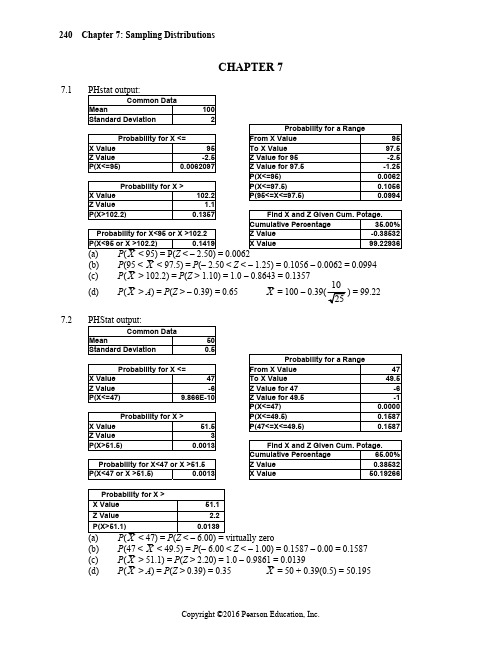
240 Chapter 7: Sampling DistributionsCHAPTER 77.1 PHstat output:Common DataMean 100Standard Deviation 2Probability for a RangeProbability for X <= From X Value 95 X Value 95To X Value 97.5 Z Value -2.5Z Value for 95 -2.5 P(X<=95) 0.0062097Z Value for 97.5 -1.25P(X<=95) 0.0062 Probability for X > P(X<=97.5) 0.1056 X Value 102.2P(95<=X<=97.5) 0.0994 Z Value 1.1P(X>102.2) 0.1357Find X and Z Given Cum. Pctage.Cumulative Percentage 35.00%Z Value -0.38532X Value 99.22936(b) P(95 < X < 97.5) = P(– 2.50 < Z < – 1.25) = 0.1056 – 0.0062 = 0.0994(c) P(X > 102.2) = P(Z > 1.10) = 1.0 – 0.8643 = 0.1357(d) P(X > A) = P(Z > – 0.39) = 0.65X = 100 – 0.39(1025) = 99.227.2 PHStat output:Common DataMean 50Standard Deviation 0.5Probability for a RangeProbability for X <= From X Value 47 X Value 47To X Value 49.5 Z Value -6Z Value for 47 -6 P(X<=47) 9.866E-10Z Value for 49.5 -1P(X<=47) 0.0000 Probability for X > P(X<=49.5) 0.1587 X Value 51.5P(47<=X<=49.5) 0.1587 Z Value 3P(X>51.5) 0.0013Find X and Z Given Cum. Pctage.Cumulative Percentage 65.00% Probability for X<47 or X >51.5 Z Value 0.38532 P(X<47 or X >51.5) 0.0013X Value 50.19266(b) P(47 < X < 49.5) = P(– 6.00 < Z < – 1.00) = 0.1587 – 0.00 = 0.1587(c) P(X > 51.1) = P(Z > 2.20) = 1.0 – 0.9861 = 0.0139(d) P(X > A) = P(Z > 0.39) = 0.35 X = 50 + 0.39(0.5) = 50.195Solutions to End-of-Section and Chapter Review Problems 241 7.3 (a) For samples of 25 customer receipts for a supermarket for a year, the samplingdistribution of sample means is the distribution of means from all possible samples of 25customer receipts for a supermarket for that year.(b) For samples of 25 insurance payouts in a particular geographical area in a year, thesampling distribution of sample means is the distribution of means from all possiblesamples of 25 insurance payouts in that particular geographical area in that year.(c) For samples of 25 Call Center logs of inbound calls tracking handling time for a creditcard company during the year, the sampling distribution of sample means is thedistribution of means from all possible samples of 25 Call Center logs of inbound callstracking handling time for a credit card company during that year.7.4 (a) Sampling Distribution of the Mean for n = 2 (without replacement)iX1 1, 31X = 22 1, 62X = 3.53 1, 73X = 44 1, 94X = 55 1, 105X = 5.56 3, 66X = 4.57 3, 77X = 58 3, 98X = 69 3, 109X = 6.510 6, 710X = 6.511 6, 911X = 7.512 6, 1012X = 813 7, 913X = 814 7, 1014X = 8.515 9, 1015X = 9.5(a) Mean of All Possible Sample Means: Mean of All Population Elements:μX =9015=6136791066μ+++++==Both means are equal to 6. This property is called unbiasedness.242 Chapter 7: Sampling Distributions7.4 (b) Sampling Distribution of the Mean for n = 3 (without replacement) cont.X1 1, 3, 61X = 3 1/32 1, 3, 72X = 3 2/33 1, 3, 93X = 4 1/34 1, 3, 104X = 4 2/35 1, 6, 75X = 4 2/36 1, 6, 96X = 5 1/37 1, 6, 107X = 5 2/38 3, 6, 78X = 5 1/39 3, 6, 99X = 610 3, 6, 1010X = 6 1/311 6, 7, 911X = 7 1/312 6, 7, 1012X = 7 2/313 6, 9, 1013X = 8 1/314 7, 9, 1014X = 8 2/315 1, 7, 915X = 5 2/316 1, 7, 1016X = 617 1, 9, 1017X = 6 2/318 3, 7, 918X = 6 1/319 3, 7, 1019X = 6 2/320 3, 9, 1020X = 7 1/3μX =12020=6This is equal toμ, the population mean.(c) The distribution for n = 3 has less variability. The larger sample size has resulted in samplemeans being closer toμ.(d) (a) Sampling Distribution of the Mean for n = 2 (with replacement)Solutions to End-of-Section and Chapter Review Problems 243 7.4cont.XiX1X = 22 1, 32X = 3.53 1, 63X = 44 1, 74X = 55 1, 95X = 5.56 1, 106X = 27 3, 17X = 38 3, 38X = 4.59 3, 69X = 510 3, 710X = 611 3, 911X = 6.512 3, 1012X = 3.513 6, 113X = 4.514 6, 314X = 615 6, 615X = 6.516 6, 716X = 7.517 6, 917X = 818 6, 1018X= 419 7, 119X = 520 7, 320X = 6.521 7, 621X = 722 7, 722X = 823 7, 923X = 8.524 7, 1024X = 525 9, 125X = 626 9, 326X = 7.527 9, 627X = 828 9, 728X = 929 9, 929X = 9.530 9, 1030X = 5.531 10, 131X = 6.532 10, 332X = 833 10, 633X = 8.534 10, 734X = 9.535 10, 935X = 1036 10, 1036244 Chapter 7: Sampling Distributions 7.4 (d) (a) Mean of All Possible Mean of All cont. Sample Means: Population Elements:216636X μ== μ=1+3+6+7+7+126=6Both means are equal to 6. This property is called unbiasedness. (b) Repeat the same process for the sampling distribution of the mean for n = 3 (withreplacement). There will be 36216= different samples.6X μ= This is equal to μ, the population mean.(c) The distribution for n = 3 has less variability. The larger sample size has resulted inmore sample means being close to μ. 7.5(a)Because the population diameter of tennis balls is approximately normally distributed, the sampling distribution of samples of 9 will also be approximately normal with a mean ofX μμ== 2.63 and X σ== 0.01.(b)X(c)Upper bound: X = 2.6384Solutions to End-of-Section and Chapter Review Problems 2457.6 (a)When n = 4 , the shape of the sampling distribution of X should closely resemble the shape of the distribution of the population from which the sample is selected. Because the mean is larger than the median, the distribution of the sales price of new houses is skewed to the right, and so is the sampling distribution of X although it will be less skewed than the population.(b)If you select samples of n = 100, the shape of the sampling distribution of the sample mean will be very close to a normal distribution with a mean of $322,100 and a standarddeviation of X σ== $9,000.(c) X σ =900010090000==nσ(d)7.7 (a) X σ1==246 Chapter 7: Sampling Distributions 7.7 (b) PHStat output: cont.(c) X σ0.5==(d) With the sample size increasing from n = 25 to n = 100, more sample means will becloser to the distribution mean. The standard error of the sampling distribution of size 100 is much smaller than that of size 25, so the likelihood that the sample mean will fall within ±0.5 minutes of the mean is much higher for samples of size 100 (probability = 0.6827) than for samples of size 25 (probability = 0. 3829).7.8(b) P (X < A ) = P (Z < 1.0364) = 0.85 X = 27 + 1.0364 (1) = 28.0364(c) To be able to use the standard normal distribution as an approximation for the area underthe curve, we must assume that the population is symmetrically distributed such that the central limit theorem will likely hold for samples of n = 16.(d)X = 27 + 1.0364 (0.5) = 27.5182Solutions to End-of-Section and Chapter Review Problems 2477.9 (a)p = 48/64 = 0.75(b)p σ =64)30.0(70.0 = 0.05737.10 (a)p = 20/50 = 0.40(b)p σ= 7.11 (a) p = 14/40 = 0.35(b)p σ =40)70.0(30.0 = 0.07257.12 (a) 0.501p μπ==, 0.05p σ===Partial PHstat output:Probability for X > X Value 0.55Z Value 0.98P(X>0.55) 0.1635P (p > 0.55) = P (Z > 0.98) = 1 – 0.8365 = 0.1635(b) 0.60p μπ==, 0.04899p σ===Partial PHstat output:Probability for X > X Value 0.55Z Value -1.020621P(X>0.55) 0.8463P (p > 0.55) = P (Z > – 1.021) = 1 – 0.1539 = 0.8461(c) 0.49p μπ==, 0.05p σ===Partial PHstat output:Probability for X > X Value 0.55Z Value 1.2002401P(X>0.55) 0.1150P (p > 0.55) = P (Z > 1.20) = 1 – 0.8849 = 0.1151(d) Increasing the sample size by a factor of 4 decreases the standard error by a factor of 2.248 Chapter 7: Sampling Distributions7.12 (d) (a) Partial PHstat output:cont.Probability for X >X Value 0.55Z Value 1.9600039P(X>0.55) 0.0250P(p > 0.55) = P (Z > 1.96) = 1 – 0.9750 = 0.0250(b) Partial PHstat output:Probability for X >X Value 0.55Z Value -2.041241P(X>0.55) 0.9794P(p > 0.55) = P (Z > – 2.04) = 1 – 0.0207 = 0.9793(c) Partial PHstat output:Probability for X >X Value 0.55Z Value 2.4004801P(X>0.55) 0.0082P(p > 0.55) = P (Z > 2.40) = 1 – 0.9918 = 0.0082If the sample size is increased to 400, the probably in (a), (b) and (c) is smaller,larger, and smaller, respectively because the standard error of the samplingdistribution of the sample proportion becomes smaller and, hence, the samplingdistribution is more concentrated around the true population proportion.7.13 (a) Partial PHstat output:Probability for a RangeFrom X Value 0.5To X Value 0.6Z Value for 0.5 0Z Value for 0.6 2.828427P(X<=0.5) 0.5000P(X<=0.6) 0.9977P(0.5<=X<=0.6) 0.4977P(0.50 < p < 0.60) = P(0 < Z < 2.83) = 0.4977(b) Partial PHstat output:Find X and Z Given Cum. Pctage.Cumulative Percentage 95.00%Z Value 1.644854X Value 0.558154P(– 1.645 < Z < 1.645) = 0.90p = .50 – 1.645(0.0354) = 0.4418 p = .50 + 1.645(0.0354) = 0.5582(c) Partial PHstat output:Probability for X >X Value 0.65Z Value 4.2426407P(X>0.65) 0.0000P(p > 0.65) = P (Z > 4.24) = virtually zeroSolutions to End-of-Section and Chapter Review Problems 2497.13 (d)Partial PHstat output:cont.Probability for X > X Value 0.6Z Value 2.8284271P(X>0.6) 0.0023If n = 200, P (p > 0.60) = P (Z > 2.83) = 1.0 – 0.9977 = 0.0023Probability for X > X Value 0.55Z Value 3.1622777P(X>0.55) 0.00078If n = 1000, P (p > 0.55) = P (Z > 3.16) = 1.0 – 0.99921 = 0.00079More than 60% correct in a sample of 200 is more likely than more than 55% correct in asample of 1000.7.14 (a) ==πμp 0.80, ()np ππσ−=1(b)(c)250 Chapter 7: Sampling Distributions 7.14 (d) ==πμp 0.80, ()n p ππσ−=1cont.(b)(c)7.15 (a) ==πμp 0.57, ()np ππσ−=1 = 0.0495(b)Solutions to End-of-Section and Chapter Review Problems 2517.15 (c)(d) ==πμp 0.57, ()np ππσ−=1 = 0.0248(a)(b)(c)7.16 (a)population proportion and, hence,π=0.15. Also the sampling distribution of the sample proportion will be close to a normal distribution according to the central limit theorem.252 Chapter 7: Sampling Distributions7.16p μπ==0.15,p σ=== 0.0252cont. P (0.12 < p < 0.18) = P (-1.1882< Z < 1.1882) = 0.7652A = 0.1085B = 0.1915A = 0.1005B = 0.1995 7.17 (a) p μπ==0.49, p σ=== 0.0500A = 0.4078B = 0.5722Solutions to End-of-Section and Chapter Review Problems 2537.17 (c)Partial PHStat output:cont.A = 0.3920B = 0.5880(d) (a) p μπ==0.49, p σ=== 0.02500.6007A = 0.4489B = 0.5311 (c)A = 0.4410B = 0.5390254 Chapter 7: Sampling Distributions 7.18 (a) ==πμp 0.36, ()n p ππσ−=1= 0.0480(b)= 0.0240(c)Increasing the sample size by a factor of 4 decreases the standard error by a factor of . The sampling distribution of the proportion becomes more concentrated around the true proportion of 0.36 and, hence, the probability in (b) becomes smaller than that in (a).7.19 Because the average of all the possible sample means of size n is equal to the population mean.7.20 The variation of the sample means becomes smaller as larger sample sizes are taken. This is dueto the fact that an extreme observation will have a smaller effect on the mean in a larger sample than in a small sample. Thus, the sample means will tend to be closer to the population mean as the sample size increases.7.21 As larger sample sizes are taken, the effect of extreme values on the sample mean becomessmaller and smaller. With large enough samples, even though the population is not normally distributed, the sampling distribution of the mean will be approximately normally distributed.7.22 The population distribution is the distribution of a particular variable of interest, while thesampling distribution represents the distribution of a statistic.7.23 When the items of interest and the items not of interest are at least 5, the normal distribution canbe used to approximate the binomial distribution.Solutions to End-of-Section and Chapter Review Problems 2557.24 0.753X μ=5004.0==nX σσ = 0.0008PHStat output:Common DataMean 0.753 Standard Deviation 0.0008Probability for a RangeProbability for X <=From X Value 0.75 X Value 0.74 To X Value 0.753 Z Value -16.25 Z Value for 0.75 -3.75 P(X<=0.74) 1.117E-59 Z Value for 0.753 0P(X<=0.75) 0.0001 Probability for X >P(X<=0.753) 0.5000 X Value 0.76 P(0.75<=X<=0.753) 0.4999 Z Value 8.75P(X>0.76) 0.0000 Find X and Z Given Cum. Pctage.Cumulative Percentage 7.00% Probability for X<0.74 or X >0.76 Z Value -1.475791 P(X<0.74 or X >0.76) 0.0000X Value 0.751819Probability for a Range From X Value 0.74 To X Value 0.75 Z Value for 0.74 -16.25 Z Value for 0.75 -3.75 P(X<=0.74) 0.0000 P(X<=0.75) 0.0001 P(0.74<=X<=0.75) 0.00009(a) P (0.75 < X < 0.753) = P (– 3.75 < Z < 0) = 0.5 – 0.00009 = 0.4999 (b) P (0.74 < X < 0.75) = P (– 16.25 < Z < – 3.75) = 0.00009 (c) P (X > 0.76) = P (Z > 8.75) = virtually zero (d) P (X < 0.74) = P (Z < – 16.25) = virtually zero (e) P (X < A ) = P (Z < – 1.48) = 0.07 X = 0.753 – 1.48(0.0008) = 0.7518256 Chapter 7: Sampling Distributions 7.25 2.0X μ=505.0==nX σσ = 0.01PHStat output:Common DataMean 2 Standard Deviation 0.01Probability for a RangeProbability for X <= From X Value 1.99X Value 1.98 To X Value 2Z Value -2 Z Value for 1.99 -1P(X<=1.98) 0.0227501 Z Value for 2 0P(X<=1.99) 0.1587Probability for X >P(X<=2) 0.5000X Value 2.01 P(1.99<=X<=2) 0.3413Z Value 1P(X>2.01) 0.1587 Find X and Z Given Cum. Pctage.Cumulative Percentage 1.00%Probability for X<1.98 or X>2.01Z Value-2.326348P(X<1.98 or X >2.01) 0.1814 X Value 1.976737Find X and Z Given Cum. Pctage.Cumulative Percentage 99.50% Z Value 2.575829X Value2.025758(a) P (1.99 < X < 2.00) = P (– 1.00 < Z < 0) = 0.5 – 0.1587 = 0.3413 (b) P (X < 1.98) = P (Z < – 2.00) = 0.0228(c) P (X > 2.01) = P (Z > 1.00) = 1.0 – 0.8413 = 0.1587(d) P (X > A ) = P ( Z > – 2.33) = 0.99 A= 2.00 – 2.33(0.01) = 1.9767 (e) P (A < X < B ) = P (– 2.58 < Z < 2.58) = 0.99A = 2.00 – 2.58(0.01) = 1.9742B = 2.00 + 2.58(0.01) = 2.0258Solutions to End-of-Section and Chapter Review Problems 2577.26 4.7X μ=0.400.085X σ===PHstat output:Common DataMean 4.7 Standard Deviation 0.08Probability for X >Find X and Z Given Cum. Pctage. X Value 4.6 Cumulative Percentage 23.00% Z Value -1.25 Z Value -0.738847 P(X>4.6) 0.8944 X Value 4.640892Find X and Z Given Cum. Pctage. Find X and Z Given Cum. Pctage. Cumulative Percentage 15.00% Cumulative Percentage 85.00% Z Value -1.036433 Z Value 1.036433 X Value 4.6170853X Value 4.782915(a) P (4.60 < X ) = P (– 1.25 < Z ) = 1 – 0.1056 = 0.8944 (b) P (A < X < B ) = P (– 1.04 < Z < 1.04) = 0.70A = 4.70 – 1.04(0.08) = 4.6168 ounces X = 4.70 + 1.04(0.08) = 4.7832 ounces(c) P (X > A ) = P (Z > – 0.74) = 0.77A = 4.70 – 0.74(0.08) = 4.6408 7.27X μ=5.00.400.085X σ===(a)Partial PHStat output:Probability for X > X Value 4.6 Z Value -5 P(X>4.6)1.0000P (4.60 < X ) = P (– 5 < Z ) = essentially 1.0 (b) Partial PHStat output:Find X and Z Given Cum. Pctage. Cumulative Percentage 15.00% Z Value -1.036433 X Value 4.917085A = 5.0 – 1.0364(0.08) = 4.9171 ounces X = 5.0 + 1.0364(0.08) = 5.0829 ounces258 Chapter 7: Sampling Distributions7.27 (c) Partial PHStat output: cont.Find X and Z Given Cum. Pctage. Cumulative Percentage 23.00% Z Value -0.738847 X Value4.940892P (X > A ) = P (Z > – 0.7388) = 0.77 A = 5.0 – 0.7388(0.08) = 4.94097.28 μμ=X = 15.23, X σ=(a)(b)(c)7.29 (a) μ=3.17 σ = 10Solutions to End-of-Section and Chapter Review Problems 2597.29 (b)Partial PHStat output:cont.(c)(d) μμ=X= 3.17, X σ== 5(e)(f)(g)Since the sample mean of returns of a sample of stocks is distributed closer to the population mean than the return of a single stock, the probabilities in (a) and (b) are higher than those in (d) and (e) while the probability in (c) is lower than that in (f).。

商务统计学课件英文版BSFC7e-CH01

Chapter 1, Slide 5
Collecting Data Correctly Is A Critical
Task
DCOVA
▪ Need to avoid data flawed by biases, ambiguities, or other types of errors.
▪ Results from flawed data will be suspect or in error.
Chapter 1, Slide 2
Classifying Variables By Type
DCOVA
▪ Categorical (qualitative) variables take categories as their values such as “yes”, “no”, or “blue”, “brown”, “green”.
Copyright © 2016, 2013, 2010 Pearson Education, Inc.
Chapter 1, Slide 7
Establishing A Business Objective
Focuses Data Collection
Examples Of Business Objectives:
People being surveyed to determine their satisfaction with a recent product or service experience.
Copyright © 2016, 2013, 2010 Pearson Education, Inc.
Chapter 1, Slide 12
Examples of Survey Data

商务统计相关知识(英文版)

If the population is believed to be at least approximately normal, a sample size of less than 15 can be used.
Interval Estimate of Population Mean:
s Known
Equation (7.1) does not say that the probability of true
lying between the given limits is 1 − α.
Since , although an unknown, is assumed to be some fixed
Interval Estimate of a Population Mean:
s Known
Adequate Sample Size (continued)
If the population is not normally distributed but is roughly symmetric, a sample size as small as 15 will suffice.
Point Estimate +/- Margin of Error
The purpose of an interval estimate is to provide information about how close the point estimate is to the value of the parameter.
s is rarely known exactly, but often a good estimate
can be obtained based on historical data or other information.

《统计学基础(英文版·第7版)》课件les7e_ppt_ADA_0304

Slide 17
Example: Finding Probabilities (2 of 3)
Find the probability of being dealt 5 diamonds from a standard deck of 52 playing cards.
Solution In a standard deck of playing cards, 13 cards are diamonds. Note that it does not matter what order the cards are selected. The possible number of ways of choosing 5 diamonds out of 13 is 13C5.
Slide 7
Example: Finding presubscript n P subscript r (1 of 2)
Find the number of ways of forming four-digit codes in which no digit is repeated.
Solution:
• You need to select 4 digits from a group of 10
•
n 10, r 4
10
P4
10
10 4
10 6
10 9 8 7 6 6
5040 ways
Copyright 2019, 2015, 2012, Pearson Education, Inc.
Solution: The number of permutations is
9 9 8 7 6 5 4 3 2 1 362,880 ways

--summary statistics(商务统计英文版) ppt课件

BEO1106 - Week 2
4
2. MEASURES OF VARIABILITY (DISPERSION)
– How much is the data spread out around its centre?
• Range: largest – smallest
Properties of the range:
• Variance:
‘average’ of the squared deviations from the mean.
For the population: 2 (sigma)
N
(xi μ)2
σ 2 i1 N
Sum of squared deviations
divided by N, n-1
ห้องสมุดไป่ตู้
Uncharacteristically small or large values.
• Median:
The middle value of an ordered array.
50%
50%
smallest
Median
BEO1106 - Week 2
largest
3
How to find the median ‘manually’? i. Sort the data from smallest to largest. ii. Choose the middle value if n (N) is odd, or take the average of the two middle values if n (N) is even.
– It has limited application and mathematical potential.

商务统计全英Chapter 7

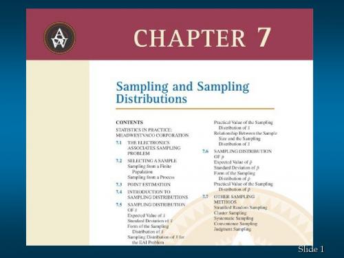
The target population is the population we want to make inferences about.
Slide 6
Simple Random Sampling From a Finite Population

Finite populations are often defined by lists such as: • Organization membership roster • Credit card account numbers • Inventory product numbers A simple random sample of size n from a finite population of size N is a sample selected such that each possible sample of size n has the same probability of being selected.
Slide 13
Example: St. Andrew’s
We will now look at two alternatives for obtaining the desired information. Conducting a census of the entire 900 applicants Selecting a sample of 30 applicants, using Excel
Slide 11
Example: St. Andrew’s
St. Andrew’s College receives 900 applications annually from prospective students. The application form contains a variety of information including the individual’s scholastic aptitude test (SAT) score and whether or not the individual desires on-campus housing.

business statistics_ppt_ch07

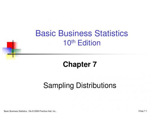
Basic Business Statistics, 10e © 2006 Prentice-Hall, Inc.
_
X
Chap 7-8
(no longer uniform)
Developing a Sampling Distribution
(continued)
Summary Measures of this Sampling Distribution:
Basic Business Statistics, 10e © 2006 Prentice-Hall, Inc.
Developing a Sampling Distribution
(continued)
Sampling Distribution of All Sample Means
16 Sample Means
μX
X
N
i
18 19 21 24 21 16
σX
( Xi μ X )2 N (18 - 21)2 (19 - 21)2 (24 - 21)2 1.58 16
Chap 7-9
Basic Business Statistics, 10e © 2006 Prentice-Hall, Inc.
Larger sample size
μ
Basic Business Statistics, 10e © 2006 Prentice-Hall, Inc.
x
Chap 7-16
If the Population is not Normal
We can apply the Central Limit Theorem:
μX μ
and

英文商务统计学ppt_第七章Ch07

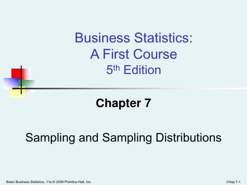
Simple Random
Stratified Cluster
Systematic
Basic Business Statistics, 11e © 2009 Prentice-Hall, Inc..
Chap 7-5
Types of Samples: Nonprobability Sample

In a nonprobability sample, items included are chosen without regard to their probability of occurrence.

Every individual or item from the frame has an equal chance of being selected
Selection may be with replacement (selected individual is returned to frame for possible reselection) or without replacement (selected individual isn’t returned to the frame). Samples obtained from table of random numbers or computer random number generators.

Basic Business Statistics, 11e © 2009 Prentice-Hall, Inc..
Chap 7-3
A Sampling Process Begins With A Sampling Frame

The sampling frame is a listing of items that make up the population Frames are data sources such as population lists, directories, or maps Inaccurate or biased results can result if a frame excludes certain portions of the population Using different frames to generate data can lead to dissimilar conclusions

商务统计学ppt课件

精选ppt课件
17
统计的应用领域
hydrology(水文学)
industry(工学)
linguistics(语言学)
literature(文学)
manpower planning(劳动力计划)
management science(管理科学)
marketing(市场营销学)
medical diagnosis(医学诊断)
称
离散变量：取有限个值连续变量：可以取无穷多个值
精选ppt课件
30
统计中的几个基本概念
总体（参数）平均数 μ 标准差 σ 比例 Π
样本（统计量） ¯x s p
精选ppt课件
31
几个常用的统计软件（software）
典型的统计软件
SAS SPSS MINITAB STATISTICA EXCEL
所研究的全部元素的集合，其中的每一个元素称为个体
分为有限总体和无限总体
有限总体的范围能够明确确定，且元素的数目是有限的无限总体所包括的元素是无限的，不可数的
2、样本（sample）
从总体中抽取的一部分元素的集合构成样本的元素的数目称为样本容量
精选ppt课件
28
参数和统计量
1、参数（parameter）
商务统计学 Business Statistics
精选ppt课件
1
参考书籍：
• 商务统计学戴维.M.莱文等著贾俊平改编
•
中国人民大学出版社
• 统计学原理谢启南主编暨南大学出版社
• 统计学原理贾俊平中国人民大学出版社
精选ppt课件
2
成绩评定方法
• 1.闭卷考试成绩（70%） • 2.平时作业、考勤和上机。（30%）

商务统计,英文版

Business Statistics
BEO 1106
WEEK 1 INTRODUCTION TO STATISTICS
PRESENTATION OF DATA
Reference: Selvanathan et al. (2004), Chapters 1, 2
SUBJECT INFORMATION
Text: Selvanathan, A et al. (2004): Australian Business Statistics, 3rd edition (Abridged), Nelson.
BEO1106 - Week 1 2
Assessment: Test/Case Study (in week 6 tutorials, closed book) Assignment (in groups of 2 students) Examination (3 hours, multiple choice, open book) Total
20% 20% 60% 100%
To pass this subject you must complete each of the above assessments, obtain at least 30 out of 60 in the examination and obtain at least 50 out of 100 in total. To obtain a satisfactory mark in this subject you should attend: Lectures: 2 hours Tutorials: 1 hour Workshops : 1 hour (Optional) and devote about 6 hours a week to independent learning, which should include revising lecture material, reading the chapters of the text book, attempting recommended questions and completing assignment tasks each week.

戴维商务统计学第7版英文版教学课件BSFC7e_CH00

Marketers driving loyalty programs and customer marketing decisions to drive sales.
Supply chain managers planning and forecasting based on product distribution and optimizing sales distribution based on key inventory measures.
Summarize & visualize business data
Reach conclusions from those data
Make reliable predictions about business activities
Improve business processes
Copyright © 2016, 2013, 2010 Pearson Education, Inc.
Copyright © 2016, 2013, 2010 Pearson Education, Inc.
Chapter GS, Slide 12
The Growth Of “Big Data” Spurs The Use Of Business Analytics
“Big Data” is still a fuzzy concept.
Chapter GS, Slide 5
To Properly Apply Statistics You Should Follow A Framework To Minimize Possible Errors
In this book we will use DCOVA

商务统计学ppt sbfc1e_alq_chapter07

Game Commercials Won't Watch
Total
Male 279 81 132
492
Female 200 156 160
516
Total 479 237 292
1008
What is the marginal probability that a viewer was female?
A. .159
B. .310
C. .643
D. .512
Game Commercials Won't Watch
Total
Male 279 81 132
492
Female 200 156 160
516
Total 479 237 292
1008
What is the marginal probability that a viewer was female?
A. True
B. False
Copyright © 2011 Pearson Education, Inc.
Slide 7- 6
For independent trials, the Law of Averages states that as the number of trials increases, the long run relative frequency of repeated events gets closer and closer to a single value.
A. less than 50%, since “tails” are due to come up. B. 50%. C. greater than 50%, since it appears that we are in a streak of “heads.” D. not able to be determined.

商务英语 PPT提纲

P1SEVEN:my favorite movie of David Fincher 标题P21 who is the dirrcter2 who take part in this film3 what story the film sayP3David Fincher (born August 28, 1962) is an American film and music v ideo director.Known f or his dark thrillers, such as Seven (1995), The Game (1997), Fight Club (1999),, and Zodiac (2007),这里放一张导演大卫芬奇的照片下面列出来他的作品就行了。

Fincher receivedAcademy Award nominations for Best Director for his 2008 film The Curious Case of Benjamin Button and his 2010 film The Social Netw ork, whi c h also w on him the Golden Globe and the BAFT A for Best Director.P4but some other f ilms are f amous too,such as The Curious Case of Benjamin Button(2007) and The Social Network at last year, I think it is Worthy of the oscar.这里列出来这两部电影的海报William Bradley "Brad" Pitt[1] (born December 18, 1963) is an American actor and f ilm producer. Pitt has receiv ed two Academy Award nominations and f our Golden Globe Award nominations, winning one. He has been described as one of the world's most attractiv e men, a label f or which he has receiv ed substantial media attentionIn 1995, Pitt starred alongside Morgan Freeman and Gwy neth Paltrow in the crime thriller Seven, play ing a detectiv e on the trail of a serial killer (play ed by Kev in Spacey).[38]Pitt called the f ilm a great mov ie and declared the part would expand his acting horizons,[39] expressing a desire to mov e on f rom "this 'pretty boy' thing [...] and play someone with f laws".[40] His perf ormance was critically well-receiv ed, with Variety say ing that it was screen acting at its best, f urther remarking on Pitt's ability to turn in a "determined, energetic, creditable job" as the detectiv e.[41]Seven earned $327 million at the international box office.P5据说David Fincher正在策划将乔治奥威尔的《1984》改变成电影，并将于2012年上映，我非常期待这部电影，但是我想大家可能不能在电影院里看到这部电影了。