多恩布什宏观经济学第十版课后习题答案04
多恩布什宏观经济学第十版课后习题答案03
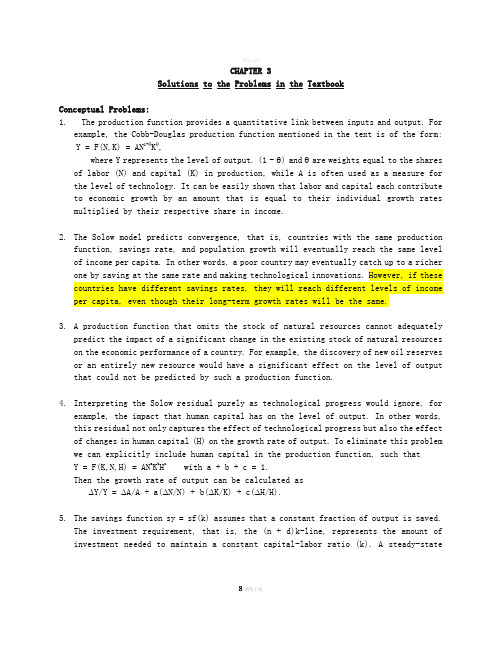
CHAPTER 3Solutions to the Problems in the TextbookConceptual Problems:1. The production function provides a quantitative link between inputs and output. Forexample, the Cobb-Douglas production function mentioned in the text is of the form: Y = F(N,K) = AN1-θKθ,where Y represents the level of output. (1 - θ) and θare weights equal to the shares of labor (N) and capital (K) in production, while A is often used as a measure for the level of technology. It can be easily shown that labor and capital each contribute to economic growth by an amount that is equal to their individual growth rates multiplied by their respective share in income.2. The Solow model predicts convergence, that is, countries with the same productionfunction, savings rate, and population growth will eventually reach the same level of income per capita. In other words, a poor country may eventually catch up to a richer one by saving at the same rate and making technological innovations. However, if these countries have different savings rates, they will reach different levels of income per capita, even though their long-term growth rates will be the same.3. A production function that omits the stock of natural resources cannot adequatelypredict the impact of a significant change in the existing stock of natural resources on the economic performance of a country. For example, the discovery of new oil reserves or an entirely new resource would have a significant effect on the level of output that could not be predicted by such a production function.4. Interpreting the Solow residual purely as technological progress would ignore, forexample, the impact that human capital has on the level of output. In other words, this residual not only captures the effect of technological progress but also the effect of changes in human capital (H) on the growth rate of output. To eliminate this problem we can explicitly include human capital in the production function, such that Y = F(K,N,H) = AN a K b H c with a + b + c = 1.Then the growth rate of output can be calculated as∆Y/Y = ∆A/A + a(∆N/N) + b(∆K/K) + c(∆H/H).5. The savings function sy = sf(k) assumes that a constant fraction of output is saved.The investment requirement, that is, the (n + d)k-line, represents the amount of investment needed to maintain a constant capital-labor ratio (k). A steady-stateequilibrium is reached when saving is equal to the investment requirement, that is, when sy = (n + d)k. At this point the capital-labor ratio k = K/N is not changing, so capital (K), labor (N), and output (Y) all must be growing at the same rate, that is, the rate of population growth n = (∆N/N).6. In the long run, the rate of population growth n = (∆N/N) determines the growth rateof the steady-state output per capita. In the short run, however, the savings rate, technological progress, and the rate of depreciation can all affect the growth rate.7. Labor productivity is defined as Y/N, that is, the ratio of output (Y) to labor input(N). A surge in labor productivity therefore occurs if output grows at a faster rate than labor input. In the U.S. we have experienced such a surge in labor productivity since the mid-1990s due to the enormous growth in GDP. This surge can be explained from the introduction of new technologies and more efficient use of existing technologies. Many claim that the increased investment in and use of computer technology has stimulated economic growth. Furthermore, increased global competition has forced many firms to cut costs by reorganizing production and eliminating some jobs. Thus, with large increases in output and a slower rate of job creation we should expect labor productivity to increase. (One should also note that a higher-skilled labor force also can contribute to an increase in labor productivity, since the same number of workers can produce more output if workers are more highly skilled.)Technical Problems:1.a. According to Equation (2), the growth of output is equal to the growth in labortimes the labor share plus the growth of capital times the capital share plus the rate of technical progress, that is,∆Y/Y = (1 - θ)(∆N/N) + θ(∆K/K) + ∆A/A, where1 - θis the share of labor (N) and θis the share of capital (K). Thus if we assumethat the rate of technological progress (∆A/A) is zero, then output grows at an annual rate of 3.6 percent, since∆Y/Y = (0.6)(2%) + (0.4)(6%) + 0% = 1.2% + 2.4% = + 3.6%,1.b. The so-called "Rule of 70" suggests that the length of time it takes for outputto double can be calculated by dividing 70 by the growth rate of output. Since 70/3.6 = 19.44, it will take just under 20 years for output to double at an annual growth rate of 3.6%,1.c. Now that ∆A/A = 2%, we can calculate economic growth as∆Y/Y = (0.6)(2%) + (0.4)(6%) + 2% = 1.2% + 2.4% + 2% = + 5.6%.Thus it will take 70/5.6 = 12.5 years for output to double at this new growth rateof 5.6%.2.a. According to Equation (2), the growth of output is equal to the growth in labortimes the labor share plus the growth of capital times the capital share plus the growth rate of total factor productivity (TFP), that is,∆Y/Y = (1 - θ)(∆N/N) + θ(∆K/K) + ∆A/A, where1 - θ is the share of labor (N) and θ is the share of capital (K). In this exampleθ = 0.3; therefore, if output grows at 3% and labor and capital grow at 1% each, then we can calculate the change in TFP in the following way3% = (0.3)(1%) + (0.7)(1%) + ∆A/A ==> ∆A/A = 3% - 1% = 2%,that is, the growth rate of total factor productivity is 2%.2.b. If both labor and the capital stock are fixed and output grows at 3%, then allthis growth has to be contributed to the growth in factor productivity, that is, ∆A/A = 3%.3.a. If the capital stock grows by ∆K/K = 10%, the effect on output would be an additionalgrowth rate of∆Y/Y = (.3)(10%) = 3%.3.b. If labor grows by ∆N/N = 10%, the effect on output would be an additional growthrate of∆Y/Y = (.7)(10%) = 7%.3.c. If output grows at ∆Y/Y = 7% due to an increase in labor by ∆N/N = 10%, and thisincrease in labor is entirely due to population growth, then per capita income would decrease and people’s welfare would decrease, since∆y/y = ∆Y/Y - ∆N/N = 7% - 10% = - 3%.3.d. If this increase in labor is due to an influx of women into the labor force, theoverall population does not increase and income per capita would increase by ∆y/y = 7%. Therefore people's welfare would increase.4. Figure 3-4 shows output per head as a function of the capital-labor ratio, that is,y = f(k). The savings function is sy = sf(k), and it intersects the straight (n + d)k-line, representing the investment requirement. At this intersection, the economy is in a steady-state equilibrium. Now let us assume that the economy is in a steady-state equilibrium before the earthquake hits, that is, the steady-state capital-labor ratio is currently k*. Assume further, for simplicity, that the earthquake does not affect people's savings behavior.If the earthquake destroys one quarter of the capital stock but less than one quarterof the labor force, then the capital-labor ratio falls from k*to k1 and per-capita output falls from y*to y1. Now saving is greater than the investment requirement, that is, sy1 > (d + n)k1, and the capital stock and the level of output per capita will grow until the steady state at k* is reached again.However, if the earthquake destroys one quarter of the capital stock but more than one quarter of the labor force, then the capital-labor ratio increases from k* to k2.Saving now will be less than the investment requirement and thus the capital-labor ratio and the level of output per capita will fall until the steady state at k*is reached again.If exactly one quarter of both the capital stock and the labor stock are destroyed, then the steady state is maintained, that is, the capital-labor ratio and the output per capita do not change.If the severity of the earthquake has an effect on peoples’savings behavior, then the savings function sy = sf(k) will move either up or down, depending on whether the savings rate (s) increases (if people save more, so more can be invested in an effort to rebuild) or decreases (if people save less, since they decide that life is too short not to live it up).yy = f(k)y2y* (n+d)ky1syk1 k* k2 k5.a. An increase in the population growth rate (n) affects the investment requirement,and the (n + d)k-line gets steeper. As the population grows, more saving must be used to equip new workers with the same amount of capital that the existing workers already have. Therefore output per capita (y) will decrease as will the new optimal capital-labor ratio, which is determined by the intersection of the sy-curve and the (n1+ d)k-line. Since per-capita output will fall, we will have a negative growth rate in the short run. However, the steady-state growth rate of output will increase in the long run, since it will be determined by the new and higher rate of population growth.y (n 1 + d)ky = f(k)y o (n o + d)ky1 syk1 k o k5.b. Starting from an initial steady-state equilibrium at a level of per-capita outputy*, the increase in the population growth rate (n) will cause the capital-labor ratio to decline from k* to k1. Output per capita will also decline, a process that will continue at a diminishing rate until a new steady-state level is reached at y1. The growth rate of output will gradually adjust to the new and higher level n1.yy*y1t o t1 tkk*k1t o t1 t6.a. Assume the production function is of the formY = F(K, N, Z) = AK a N b Z c ==>∆Y/Y = ∆A/A + a(∆K/K) + b(∆N/N) + c(∆Z/Z), with a + b + c = 1.Now assume that there is no technological progress, that is, ∆A/A = 0, and that capital and labor grow at the same rate, that is, ∆K/K = ∆N/N = n. If we also assume that all natural resources available are fixed, such that ∆Z/Z = 0, then the rate of output growth will be∆Y/Y = an + bn = (a + b)n.In other words, output will grow at a rate less than n since a + b < 1. Therefore output per worker will fall.6.b. If there is technological progress, that is, ∆A/A > 0, then output will grow fasterthan before, namely∆Y/Y = ∆A/A + (a + b)n.If ∆A/A > c, then output will grow at a rate larger than n, in which case output per worker will increase.6.c. If the supply of natural resources is fixed, then output can only grow at a ratethat is smaller than the rate of population growth and we should expect limits to growth as we run out of natural resources. However, if the rate of technological progress is sufficiently large, then output can grow at a rate faster than population, even if we have a fixed supply of natural resources.7.a. If the production function is of the formY = K1/2(AN)1/2,and A is normalized to 1, then we haveY = K1/2N1/2.In this case capital's and labor's shares of income are both 50%.7.b. This is a Cobb-Douglas production function.7.c. A steady-state equilibrium is reached when sy = (n + d)k.From Y = K1/2N1/2 ==> Y/N = K1/2N-1/2 ==> y = k1/2==>sk1/2= (n + d)k ==> k-1/2 = (n + d)/s = (0.07 + 0.03)/(.2) = 1/2 ==> k1/2= 2 = y ==> k = 4 .8.a. If technological progress occurs, then the level of output per capita for any givencapital-labor ratio increases. The function y = f(k) increases to y = g(k), and thus the savings function increases from sf(k) to sg(k).y g(k)y2 f(k)(n +d)ksg(k)y1sf(k)k1 k2k8.b. Since g(k) > f(k), it follows that sg(k) > sf(k) for each level of k.Therefore the intersection of the sg(k)-curve with the (n + d)k-line is ata higher level of k. The new steady-state equilibrium will now be at a higherlevel of saving and output per capita, and at a higher capital-labor ratio.8.c. After the technological progress occurs, the level of saving and investmentwill increase until a new and higher optimal capital-labor ratio is reached.The ratio of investment to capital will also increase in the transition period, since more has to be invested to reach the higher optimal capital-labor ratio.kk2k1t1 t2t9. The Cobb-Douglas production function is defined asY = F(N,K) = AN1-θKθ.The marginal product of labor can then be derived asMPN = (∆Y)/(∆N) = (1 - θ)AN-θKθ = (1 - θ)AN1-θKθ/N = = (1 - θ)(Y/N)==> labor's share of income = [MPN*(N)]/Y = (1 - θ)(Y/N)*[(N)/(Y)] =(1 - θ)欢迎您的下载,资料仅供参考!致力为企业和个人提供合同协议,策划案计划书,学习资料等等打造全网一站式需求。
(NEW)多恩布什《宏观经济学》(第10版)笔记和课后习题详解

答:总供给—总需求模型是把总需求与总供给结合在一起来分析国民收 入与价格水平的决定及其变动的国民收入决定模型。
在图1-4中,横轴代表国民收入( ),纵轴代表价格水平( ), 代 表原来的总需求曲线, 代表短期总供给曲线, 代表长期总供给曲 线。最初,经济在 点时实现了均衡,均衡的国民收入为 ,均衡的价 格水平为 。这时 点又在长期总供给曲线 上,所以, 代表充分就 业的国民收入水平。在短期内,政府通过扩张性的财政政策或货币政 策,增加了总需求,从而使总需求曲线从 向右上方平行地移动到了
(1)经济增长模型
主要解释:经济增长的源泉;各国经济增长率差异的原因;经济起飞的 原因;分析投入的积累和技术进步如何导致生活水平的提高。
(2)经济波动模型:总供给—总需求模型(如图1-1所示)
图1-1 总供给—总需求模型
总供给—总需求模型解释物价水平与产出的决定与波动。
总供给水平:现有资源和技术条件下,经济能够生产的产出量。
潜在产出水平附近接近于一条垂直的直线。
4 经济周期(business cycle)
答:经济周期又称经济波动或国民收入波动,指总体经济活动的扩张和 收缩交替反复出现的过程。现代经济学中关于经济周期的论述一般是指 经济增长率的上升和下降的交替过程,而不是经济总量的增加和减少。
一个完整的经济周期包括繁荣、衰退、萧条、复苏(也可以称为扩张、 持平、收缩、复苏)四个阶段。在繁荣阶段,经济活动全面扩张,不断 达到新的高峰。在衰退阶段,经济短时间内保持均衡后出现紧缩的趋 势。在萧条阶段,经济出现急剧的收缩和下降,很快从活动量的最高点 下降到最低点。在复苏阶段,经济从最低点恢复并逐渐上升到先前的活 动量高度,进入繁荣。衡量经济周期处于什么阶段,主要依据国民生产 总值、工业生产指数、就业和收入、价格指数、利息率等综合经济活动 指标的波动。
多恩布什《宏观经济学》课后习题详解(增长与政策)【圣才出品】
第4章增长与政策一、概念题1.绝对趋同(absolute convergence)答:绝对趋同是指不论各国的其他特征如何,穷国的人均收入增长倾向于比富国更快。
从理论上说,经济趋同可分为“绝对趋同”和“条件趋同”两种,但实证研究证明绝对趋同并不存在,而无论是在理论上,还是在现实世界中,条件趋同都是客观存在的现象。
2.规模报酬递增(increasing returns to scale)答:规模报酬递增指产量增加的比例大于各种生产要素增加的比例。
设生产函数为Q =f(L,K),则当劳动和资本投入量同时增大λ倍时,产量为aQ=f(λL,λK),a>λ表示产量增加的幅度要大于要素投入的增长幅度。
规模报酬递增的生产函数,总产量曲线凸向右下方,表示产量的增加幅度大于要素投入量的增加幅度,如图4-1所示。
图4-1 规模报酬递增图4-1中,横轴表示劳动L和资本投入量K,纵轴表示产量Q,曲线Q为总产量曲线。
当各种要素投入量由X1增加到X2时,引起产量由Q1增加到Q2,要素投入量增加了一倍,而产量的增加大于一倍。
产生规模报酬递增的主要原因是企业生产规模扩大所带来的生产效率的提高。
它可以表现为:生产规模扩大以后,企业能够利用更先进的技术和机器设备等生产要素,而较小规模的企业可能无法利用这样的技术和生产要素。
随着对较多的人力和机器的使用,企业内部的生产分工能够更加合理和专业化。
此外,人数较多的技术培训和具有一定规模的生产经营管理也可以节省成本。
3.稳定均衡(stable equilibrium)答:稳定均衡指如果经济体系的均衡状态遭到暂时破坏时,依靠其自身的力量最终还会恢复到原来所处的均衡状态的一种均衡。
其特点是一个经济体系的均衡状态,在制约它的各种外部条件发生变动时,会使该经济体系产生脱离均衡状态的运动,但是,经济体系内部又同时会自动地产生一种力量,这种力量使体系中的各种变量重新恢复到原来的均衡状态。
例如,当某一商品的供给曲线在均衡点的斜率大于需求曲线的斜率时,脱离均衡状态的波动幅度会自动逐渐缩小以至消失,并最终停留在原均衡点上,这就是阐述动态均衡的蛛网理论所描述的收敛型蛛网情况。
多恩布什《宏观经济学》(第10版)笔记和课后习题详解 第4章 增长与政策【圣才出品】
第4章增长与政策4.1复习笔记1.内生增长理论内生增长理论是指罗默、卢卡斯等经济学家提出的,用规模收益递增和内生技术进步来说明一个国家长期经济增长和各国增长率差异的一种经济增长理论。
该理论试图将增长率解释为社会决策的函数,特别是储蓄率的函数。
修改新古典增长模型中假定的生产函数的形状,在一定程度上就会出现容许自我持续的(即内生的)增长。
(1)基本假设①社会储蓄函数为S sY =,其中s 为储蓄率;②劳动增长率n 不变;③资本的边际产品不变;④存在外部经济且外部报酬相当大;⑤技术进步是内生要素,技术与总体经济中每个工人的资本水平成正比例,/A K N k αα==,并假定技术属于劳动增加型。
(2)基本方程在上述假定下,把生产函数写为()Y F K AN =,,该生产函数满足规模报酬不变。
对生产函数求全微分:()F F Y K N A A N K AN∂∂∆=⨯∆+⨯∆+⨯∆∂∂Y K F K K AN F AN N AN F AN A Y K N A∆⨯∂∂∆⨯∂∂∆⨯∂∂∆=⋅+⋅+⋅由于生产函数满足规模收益不变,要素及产品市场属于完全竞争市场,运用欧拉定理得:K F K θ⨯∂∂=,1AN F AN θ⨯∂∂=-即有:()()11Y K N Aθθθ∆∆∆∆=⨯+-⨯+-⨯人均产出增长率表达式:()1Y N K N A YN K N A θθ∆∆∆∆∆⎛⎫⎛⎫-=-⨯+⨯- ⎪ ⎪⎝⎭⎝⎭即有:()1y k A y k Aθθ∆∆∆=⨯+⨯-将技术增长公式A K N k A K N k∆∆∆∆=-=代入GDP 增长方程,得:()()11y k A k k k y k A k k kθθθθ∆∆∆∆∆∆=⨯+⨯-=+-=可以判断,y k是常数。
将生产函数除以K 可得出该常数:()()()1F K AN y F K K AN K F k Kαα===≡,,,资本积累方程为()k sy n d k k ∆=-+,联立上式可得,内生增长模型的人均产出增长率的基本公式为:()()y k sy g n d sa n d y k k∆∆===-+=-+。
多恩布什《宏观经济学》第10版课后习题详解(货币、利息与收入)【圣才出品】

5. IS 曲线( IS curve)
答: IS 曲线指将满足产品市场均衡条件的收入和利率的各种组合的点连结起来而形成
的曲线。它是反映产品市场均衡状态的一幅简单图像。它表示的是任一给定的利率水平上都
M P h h kbG
h 与 k 数值越小,b 与 G 数值越大,增加实际余额对均衡收入水平的扩张性效应也越大。 b 与 G 的数值大,对应着非常平直的 IS 曲线。
4.中央银行(central bank) 答:中央银行指在一国金融体系中居于主导地位,负责制定和执行国家的金融政策,调 节货币流通与信用活动,对国家负责,在对外金融活动中代表国家,并对国内整个金融体系 和金融活动实行管理与监督的金融中心机构。中央银行具有三大职能,即它是“发行的银行”、 “银行的银行”和“政府的银行”。
2 / 21
圣才电子书 十万种考研考证电子书、题库视频学习平台
(1)中央银行是发行的银行,这一职能指中央银行服务于社会和经济发展,供应货币、 调节货币量、管理货币流通的职能。
(2)中央银行是银行的银行,这一职能指中央银行服务于商业银行和整个金融机构体 系,履行维持金融稳定、促进金融业发展的职责。
6.货币市场的均衡曲线(money market equilibrium schedule)
3 / 21
圣才电子书 十万种考研考证电子书、题库视频学习平台
答:LM 曲线即货币市场的均衡曲线,它显示能使其实际余额需求等于供给的所有利率
与收入水平的组合。沿着 LM 曲线,货币市场处于均衡状态。要使货币市场处于均衡状态,
A bi
多恩布什《宏观经济学》第10版课后习题详解(国际调整与相互依存)【圣才出品】
多恩布什《宏观经济学》第10版课后习题详解第20章国际调整与相互依存一、概念题1.自动调节机制(automatic adjustment mechanisms)答:自动调节机制指自动起作用消除国际收支失衡问题的机制。
在纯粹的自由经济中有货币—价格机制、收入机制及利率机制等国际收支自动调节机制。
货币—价格机制,也称“价格—现金流动机制”,其描述的是国内货币供给存量与一般物价水平变动以及相对价格水平变动对国际收支的影响。
当一国处于逆差状态时,对外支付大于收入,货币外流,物价下降,本国汇率也下降,由此导致本国出口商品的价格绝对或相对下降,从而出口增加,进口减少,贸易收入得到改善。
收入机制的调节作用表现为:当国际收支逆差时,国民收入下降。
国民收入下降引起社会总需求下降,从而进口需求也下降,进而改善贸易收支。
利率机制的调节作用表现为:当国际收支发生逆差时,本国货币供给存量减少,利率因此上升,这意味着本国金融资产的收益上升,从而对本国金融资产的需求上升,对外国金融资产的需求相对下降。
这样,资金外流减少或内流增加,资本与金融项目收支得到改善。
当国际收支顺差时,上述的自动调节仍然起作用,只是方向相反而已。
2.内部和外部平衡(internal and external balance)答:内部平衡指国民经济处于无通货膨胀的充分就业状态。
内部均衡时国内产品市场、货币市场和劳动市场同时达到均衡,宏观经济处于充分就业水平上,并且没有通货膨胀的压力,经济稳定增长。
内部均衡目标包括经济增长、价格稳定和充分就业。
外部均衡指国际收支平衡,也即贸易品的供求处于均衡状态。
当国际收支平衡时,既无国际收支顺差,也无国际收支逆差。
在开放经济中,宏观经济的最终目标是实现内部均衡和外部均衡。
英国经济学家詹姆斯·米德开创性地提出了“两种目标、两种工具”的理论模式,即在开放经济条件下,一国经济如果希望同时达到对内均衡和对外均衡的目标,则必须同时运用支出增减政策和支出转换政策两种工具。
多恩布什《宏观经济学》第10版课后习题详解(货币政策与财政政策)【圣才出品】
多恩布什《宏观经济学》第10版课后习题详解第11章货币政策与财政政策一、概念题1.预期的货币政策(anticipatory monetary policy)答:预期的货币政策指为了对估计到的未来将会发生的问题(例如通货膨胀的压力)作出反应而采用的货币政策。
比如,在一个预先防范的货币政策的例子中,央行不是对总需求与通货膨胀压力的现有情况作出反应,而是对经济如果增长过快,会发生通货膨胀的这种担心作出反应。
该政策的基本问题是:确定货币政策时,应当往前看。
2.投资税减免(investment tax credit)答:投资税减免指国家以法律形式规定的在一定条件下允许纳税人以用于某些方面的投资抵免一定税款的政策措施。
实行这种政策,表明国家是鼓励税收减免的,即国家为支持投资而在税收方面作出优惠的减免税的规定。
这种政策对鼓励和吸引投资有一定成效。
我国在改革开放中也使用了这种政策。
3.政策组合(policy mix)答:政策组合指为了实现宏观经济目标而采取的财政政策、货币政策以及其他一些政策工具的组合。
扩张性的财政政策表现为IS曲线右移,在使收入增加的同时会带来利率的上升,而扩张性的货币政策表现为LM曲线右移,在使收入增加的同时会带来利率的下降。
因此,为实现收入和利率的不同组合,将两种政策搭配使用,即财政政策和货币政策的混合使用。
政府和中央银行可以根据具体情况和不同目标,选择不同的政策组合。
例如,当经济萧条但又不太严重时,用扩张性财政政策刺激总需求,又用紧缩性货币政策控制通货膨胀;当经济发生严重通货膨胀时,用紧缩货币来提高利率,降低总需求水平,又紧缩财政,以防止利率过分提高;当经济中出现通货膨胀又不太严重时,用紧缩财政压缩总需求,又用扩张性货币政策降低利率,以免财政政策紧缩而引起衰退;当经济严重萧条时,用扩张财政增加总需求,用扩张货币降低利率以克服“挤出效应”。
4.古典情况(classical case)答:古典情况即垂直的LM曲线,是货币需求对于实际利率十分敏感的情况。
多恩布什《宏观经济学》第10版课后习题详解(重大事件:萧条经济学、恶性通货膨胀和赤字)【圣才出品】
圣才电子书 十万种考研考证电子书、题库视频学习平台
6.可信的政策(credible policy) 答:可信的政策指人们相信政府将会遵循的政策。可信的政策有利于赢得公众的信心, 从而在最大程度上降低政策成本。政府政策的可信度不高,会降低公众对政府的信心,使得 政府无法引导公众预期,加大政策执行难度。因此,政府应该努力提高政策的可信性,合理 引导公众预期,降低政策成本。
4.信任奖励(credibility bonus) 答:信任奖励又称信誉红利,指在理性预期下政府政策的可信性所获得的报偿。政府在 降低通货膨胀的斗争中,由于公众相信政府的反通货膨胀政策会得到执行从而降低通货膨胀 预期,这样即使政策未执行也会使通货膨胀降低,从而避免经济的衰退,政府政策的可信性 便获得了报偿。 通货膨胀是由经济的基本方面(总需求与总供给的相对变动)所决定的。在恶性通货膨 胀中,货币的增长支配了所有的其他基本因素。但是,人们关于未来的预期也发挥了作用。 相信政策已经改变本身就会驱动预期的通货膨胀率下降,并且因此而引起短期的菲利普斯曲
2 / 38
圣才电子书 十万种考研考证电子书、题库视频学习平台
线向下移动。所以,在反通货膨胀的战斗中,一种可信任的政策会赢得社会对可信性的褒奖。 从美联储 1979 年 10 月改变其货币政策开始,在美国整个反通货膨胀时期,一直着重
强调政策的可信性。理性预期的一些支持者衰退。
新政的主要内容包括: (1)对工商业大量的贷款和津贴,刺激私人投资; (2)提高物价,减少农业生产,克服农产品过剩; (3)兴建公共工程,增加就业机会; (4)对失业者给予最低限度救济。 新政实施的结果使美国逐渐摆脱了危机,为千百万人提供了就业和生活的保障,使经济 不平衡状况有所改善。1935 年起所有经济指标都稳步上升,失业人数大幅度下降。新政大 多是应急措施,没有完整的理论依据,但体现了凯恩斯主义国家干预经济的思潮,反映了现 代私人垄断资本主义向国家垄断资本主义过渡这一总的趋向,对美国以后历届政府的政策影 响很大。
宏观经济学第十版第二章课后习题完美精简中文版
多恩布什宏观经济学第十版第二章课后习题答案完美中文精简版概念题1,他们作为政府雇员支取TR美元,但是不做任何工作,实际上就是加大了政府支出,GDP会增长。
2,a..厂商为经理买车应该看成投资,经理自己购买轿车则是消费。
b.雇佣配偶的行为是消费,计算GDP时会被计入;而无偿要求她担任此工作则是无形中忽略掉了消费环节,不计入GDP。
c.买美国轿车会使GDP增长,买德国车也会使GDP增加,但是会减少净出口。
3,GDP与GNP的区别在于:GNP是指一个国家(或地区)所有国民在一定时期内新生产的产品和服务价值的总和。
GNP是按国民原则核算的,只要是本国(或地区)居民,无论是否在本国境内(或地区内)居住,其生产和经营活动新创造的增加值都应该计算在内。
GDP是指一个国家(或地区)在一定时期内所有常住单位生产经营活动的全部最终成果。
GDP是按国土原则核算的生产经营的最终成果。
使用GDP计量产出更好,GDP的精确度高。
4,NDP是国内生产净值,NDP是从国内生产总值GDP中扣除资本折旧得到的。
如果用于计算产量,它比GDP更接近产品价值,但是折旧率是人来计算,所以会存在一定误差,在计算数值非常大时用GDP计算比较好。
5,GDP的增加不代表福利的增加,比如说GDP增加,同时人口也增长了,一平均,每个人的GDP没有变化。
我觉得最大的问题是人口问题,人口的增长和减少对人均GDP有影响。
6,CPI居民消费价格指数,是反映与居民生活有关的商品及劳务价格统计出来的物价变动指标,通常作为观察通货膨胀水平的重要指标。
PPI是衡量企业购买的一篮子物品和劳务的总费用。
从消费者的立场计算时我会选择用CPI计算。
7,GDP紧缩指数=(名义GDP/实际GDP) *100区别答不出。
8,物价是否翻了一倍,以及GDP紧缩指数有没有变化。
9,伤心。
以实际利率说明的,将要支付更少利息。
技术题12,b.收入增加意味着可支配收入增加,那么此时就能够购买更多的产品。
多恩布什宏观经济学第十版课后答案

宏观经济学第二章概念题1.如果政府雇用失业工人,他们曾领取TR美元的失业救济金,现在他们作为政府雇员支取TR美元,不做任何工作,GDP会发生什么情况?请解释。
答:国内生产总值指一个国家(地区)领土范围,本国(地区)居民和外国居民在一定时期内所生产和提供的最终使用的产品和劳务的价值。
用支出法计算的国内生产总值等于消费C、投资I、政府支出G和净出口NX之和。
从支出法核算角度看:C、I、NX保持不变,由于转移支付TR美元变成了政府对劳务的购买即政府支出增加,使得G增加了TR美元,GDP会由于G的增加而增加。
2.GDP和GNP有什么区别?用于计算收入/产量是否一个比另一个更好呢?为什么?答:(1)GNP和GDP的区别GNP指在一定时期内一国或地区的国民所拥有的生产要素所生产的全部最终产品(物品和劳务)的市场价值的总和。
它是本国国民生产的最终产品市场价值的总和,是一个国民概念,即无论劳动力和其他生产要素处于国内还是国外,只要本国国民生产的产品和劳务的价值都记入国民生产总值。
GDP指一定时期内一国或地区所拥有的生产要素所生产的全部最终产品(物品和劳务)的市场价值的总和。
它是一国范围内生产的最终产品,是一个地域概念。
两者的区别:在经济封闭的国家或地区,国民生产总值等于国内生产总值;在经济开放的国家或地区,国民生产总值等于国内生产总值加上国外净要素收入。
两者的关系可以表示为:GNP=GDP+[本国生产要素在其他国家获得的收入(投资利润、劳务收入)-外国生产要素从本国获得的收入]。
(2)使用GDP比使用GNP用于计量产出会更好一些,原因如下:1)从精确度角度看,GDP的精确度高;2)GDP衡量综合国力时,比GNP好;3)相对于GNP而言,GDP是对经济中就业潜力的一个较好的衡量指标。
由于美国经济中GDP和GNP的差异非常小,所以在分析美国经济时,使用这两种的任何一个指标,造成的差异都不会大。
但对于其他有些国家的经济来说明,这个差别是相当大的,因此,使用GDP作为衡量指标会更好。
10宏观经济学英文版(多恩布什)课后习题答案全解

CHAPTER 10MONEY, INTEREST, AND INCOMEAnswers to Problems in the Textbook:Conceptual Problems:1. The model in Chapter 9 assumed that both the price level and the interest rate were fixed. But the IS-LM model lets the interest rate fluctuate and determines the combination of output demanded and the interest rate for a fixed price level. It should be noted that while the upward-sloping AD-curve in Chapter 9 (the [C+I+G+NX]-line in the Keynesian cross diagram) assumed that interest rates and prices were fixed, the downward-sloping AD-curve that is derived at the end of Chapter 10 from the IS-LM model lets the price level fluctuate and describes all combinations of the price level and the level of output demanded at which the goods and money sector simultaneously are in equilibrium. 2.a. If the expenditure multiplier (α) becomes larger, the increase in equilibrium income caused by a unitchange in intended spending also becomes larger. Assume investment spending increases due to a change in the interest rate. If the multiplier α becomes larger, any increase in spending will cause a larger increase in equilibrium income. This means that the IS-curve will become flatter as the size of the expenditure multiplier becomes larger.If aggregate demand becomes more sensitive to interest rates, any change in the interest rate causes the [C+I+G+NX]-line to shift up by a larger amount and, given a certain size of the expenditure multiplier α, this will increase equilibrium income by a larger amount. As a result, the IS-curve will become flatter.2.b. Monetary policy changes affect interest rates and this leads to a change in intended spending, whichis reflected in a change in income. In 2.a. it was explained that a steep IS-curve means either that the multiplier α is small or that desired spending is not very interest sensitive. Therefore, an increase in money supply will reduce interest rates. However, this does not result in a large increase in aggregate demand if spending is very interest insensitive. Similarly, if the multiplier is small, then any change in spending will not affect output significantly. Therefore, the steeper the IS-curve, the weaker the effect of monetary policy changes on equilibrium output.3. Assume that money supply is fixed. Any increase in income will increase money demand and theresulting excess demand for money will drive the interest rate up. This, in turn, will reduce the quantity of money balances demanded to bring the money sector back to equilibrium. But if money demand is very interest insensitive, then a larger increase in the interest rate is needed to reach a new equilibrium in the money sector. As a result, the LM-curve becomes steeper.Along the LM-curve, an increase in the interest rate is always associated with an increase in income. This means that an increase in money demand (due to an increase in income) has to be offset by a decrease in the quantity of money demanded (due to an increase in the interest rate) to keep the money sector in equilibrium. But if money demand becomes more income sensitive, a smaller change in income is required for any specific change in the interest rate to keep the money sector in equilibrium. Therefore, the LM-curve becomes steeper as money demand becomes more income sensitive.4.a. A horizontal LM-curve implies that the public is willing to hold whatever money is supplied at anygiven interest rate. Therefore, changes in income will not affect the equilibrium interest rate in the money sector. But if the interest rate is fixed, we are back to the analysis of the simple Keynesian model used in Chapter 9. In other words, there is no offsetting effect (or crowding-out effect) to fiscal policy.14.b. A horizontal LM-curve implies that changes in income do not affect interest rates in the money sector.Therefore, if expansionary fiscal policy is implemented, the IS-curve shifts to the right, but the level of investment spending is no longer negatively affected by rising interest rates, that is, there is no crowding-out effect. In terms of Figure 10-3, the interest rate not longer serves as the link between the goods and assets markets.4.c. A horizontal LM-curve results if the public is willing to hold whatever money balances are suppliedat a given interest rate. This situation is called the liquidity trap. Similarly, if the Fed is prepared to peg the interest rate at a certain level, then any change in income will be accompanied by an appropriate change in money supply. This will lead to continuous shifts in the LM-curve, which is equivalent to having a horizontal LM-curve, since the interest rate will never change.5. From the material presented in the text we know that when intended spending becomes more interestsensitive, then the IS-curve becomes flatter. Now assume that an increase in the interest rate stimulates saving and therefore reduces the level of consumption. This means that now not only investment spending but also consumption is negatively affected by an increase in the interest rate. In other words, the [C+I+G+NX]-line in the Keynesian cross diagram will now shift down further than previously and the level of equilibrium income will decrease more than before. In other words, the IS-curve has become flatter.This can also be shown algebraically, since we can now write the consumption function as follows:C = C* + cYD - giIn a simple model of the expenditure sector without income taxes, the equation for aggregate demand will now beAD = A o + cY - (b + g)i.From Y = AD ==> Y = [1/(1 - c)][A o - (b + g)i] ==>i = [1/(b + g)]A o - [(1 - c)/(b + g)]YTherefore, the slope of the IS-curve has been reduced from (1 - c)/b to (1 - c)/(b + g).6. In the IS-LM model, a simultaneous decline in interest rates and income can only be caused by a shiftof the IS-curve to the left. This shift in the IS-curve could have been caused by a decrease in private spending due to negative business expectations or a decline in consumer confidence. In 1991, the economy was in a recession and firms did not want to invest in new machinery and, since consumer confidence was very low, people were not expected to increase their level of spending. In the IS-LM diagram the adjustment process can be described as follows:I o↓ ==> Y ↓ (the IS-curve shifts left) ==> m d↓ ==> i ↓ ==> I ↑ ==> Y ↑. Effect: Y ↓ and i ↓ .2ii1i221Technical Problems:1.a. Each point on the IS-curve represents an equilibrium in the expenditure sector. Therefore the IS-curvecan be derived by settingY = C + I + G = (0.8)[1 - (0.25)]Y + 900 - 50i + 800 = 1,700 + (0.6)Y - 50i ==>(0.4)Y = 1,700 - 50i ==> Y = (2.5)(1,700 - 50i) ==> Y = 4,250 - 125i.1.b. The IS-curve shows all combinations of the interest rate and the level of output such that theexpenditure sector (the goods market) is in equilibrium, that is, intended spending is equal to actual output. A decrease in the interest rate stimulates investment spending, making intended spending greater than actual output. The resulting unintended inventory decrease leads firms to increase their production to the point where actual output is again equal to intended spending. This means that the IS-curve is downward sloping.1.c. Each point on the LM-curve represents an equilibrium in the money sector. Therefore the LM-curvecan be derived by setting real money supply equal to real money demand, that is,M/P = L ==> 500 = (0.25)Y - 62.5i ==> Y = 4(500 + 62.5i) ==> Y = 2,000 + 250i.1.d. The LM-curve shows all combinations of the interest rate and level of output such that the moneysector is in equilibrium, that is, the demand for real money balances is equal to the supply of real money balances. An increase in income will increase the demand for real money balances. Given a fixed real money supply, this will lead to an increase in interest rates, which will then reduce the quantity of real money balances demanded until the money market clears. In other words, the LM-curve is upward sloping.1.e. The level of income (Y) and the interest rate (i) at the equilibrium are determined by the intersectionof the IS-curve with the LM-curve. At this point, the expenditure sector and the money sector are both in equilibrium simultaneously.From IS = LM ==> 4,250 - 125i = 2,000 + 250i ==> 2,250 = 375I ==> i = 6==> Y = 4,250 - 125*6 = 4,250 - 750 ==> Y = 3,500Check: Y = 2,000 + 250*6 = 2,000 + 1,500 = 3,5003i125 ISLM62,000 3,500 4,250 Y2.a. As we have seen in 1.a., the value of the expenditure multiplier is α= 2.5. This multiplier αisderived in the same way as in Chapter 9. But now intended spending also depends on the interest rate, so we no longer have Y = αA o, but ratherY = α(A o - bi) = (1/[1 - c + ct])(A o - bi) ==> Y = (2.5)(1,700 - 50i) = 4,250 - 125i.2.b.This can be answered most easily with a numerical example. Assume that government purchasesincrease by ∆G = 300. The IS-curve shifts parallel to the right by==> ∆IS = (2.5)(300) = 750.Therefore IS': Y = 5,000 - 125iFrom IS' = LM ==> 5,000 - 125i = 2,000 + 250i ==> 375i = 3,000 ==> i = 8==> Y = 2,000 + 250*8 ==> Y = 4,000 ==> ∆Y = 500When interest rates are assumed to be constant, the size of the multiplier is equal to α = 2.5, that is, (∆Y)/(∆G) = 750/300 = 2.5. But when interest rates are allowed to vary, the size of the multiplier is reduced to α1 = (∆Y)/(∆G) = 500/300 = 1.67.2.c. Since an increase in government purchases by ∆G = 300 causes a change in the interest rate of 2percentage points, government spending has to change by ∆G = 150 to increase the interest rate by 1 percentage point.2.d. The simple multiplier α in 2.a. shows the magnitude of the horizontal shift in the IS-curve, given achange in autonomous spending by one unit. But an increase in income increases money demand and the interest rate. The increase in the interest rate crowds out some investment spending and this has a dampening effect on income. The multiplier effect in 2.b. is therefore smaller than the multiplier effect in 2.a.3.a. An increase in the income tax rate (t) will reduce the size of the expenditure multiplier (α). But as themultiplier becomes smaller, the IS-curve becomes steeper. As we can see from the equation for the IS-curve, this is not a parallel shift but rather a rotation around the vertical intercept.Y = α(A o - bi) = [1/(1 - c + ct)](A o - bi) ==> i = (1/b)A o - (α/b)Y = (1/b)A o - (1/b)[1 - c + ct]Y 3.b. If the IS-curve shifts to the left and becomes steeper, the equilibrium income level will decrease. Ahigher tax rate reduces private spending and this will lower national income.3.c. When the income tax rate is increased, the equilibrium interest rate will also decrease. The adjustmentto the new equilibrium can be expressed as follows (see graph on the next page):t up ==> C down ==> Y down ==> m d down ==> i down ==> I up ==> Y up. Effect: Y ↓ and i ↓45i 1i 2214.a. If money demand is less interest sensitive, then the LM-curve is steeper and monetary policy changesaffect equilibrium income to a larger degree. If money supply is assumed to be fixed, the adjustment to a new equilibrium in the money sector has to come solely through changes in money demand. If money demand is less interest sensitive, any increase in money supply requires a larger increase in income and a larger decrease in the interest rate in order to bring the money sector into a new equilibrium.i ii 1 i 1 2 2i 20 120 12The adjustment process in each of the two diagrams is the same; however, in the case of a more interest-sensitive money demand (a flatter LM-curve), the change in Y and i will be smaller.(M/P) up ==> i down ==> I up ==> Y up ==> m d up ==> i up Effect: Y ↑ and i ↓Section 10-5 derives the equation for the LM-curve and the equation for the monetary policy multiplier asi = (1/h)[kY - (M/P)] and (∆Y)/∆(M/P) = (b/h)γrespectively. If money demand becomes more interest sensitive, the value of h becomes larger and the slope of the LM-curve becomes flatter, while the size of the monetary policy multiplier becomes smaller.4.b. An increase in money supply drives interest rates down. This decrease in interest rates will stimulateintended spending and thus income. If money demand becomes less interest sensitive, a larger increase in income is required to bring the money sector into equilibrium. But this implies that the overall decrease in the interest rate has to be larger, given that the interest sensitivity of spending has not changed.5. The price adjustment, that is, the movement along the AD-curve, can be explained in the followingway: With nominal money supply (M) fixed, real money balances (M/P) will decrease as the price level (P) increases. There is an excess demand for money and interest rates will rise. This will lead toa decrease in investment spending and thus the level of output demanded will decrease. In otherwords, the LM-curve will shift to the left as real money balances decrease.6. In the classical case, the AS-curve is vertical. Therefore, any increase in aggregate demand due toexpansionary monetary policy will, in the long run, not lead to any increase in output but simply lead to an increase in the price level. An increase in money supply will first shift the LM-curve to the right.This implies a shift of the AD-curve to the right. Therefore we have excess demand for goods and services and prices will begin to rise. But as the price level rises, real money balances will begin to fall again, eventually returning to their original level. Therefore, the shift of the LM-curve to the right due to the expansionary monetary policy and the resulting shift of the AD-curve will be exactly offset by a shift of the LM-curve to the left and a movement along the AD-curve to the new long-run equilibrium due to the price adjustment. At this new long-run equilibrium, the level of output and interest rates will not have changed while the price level will have changed proportionally to the nominal money supply, leaving real money balances unchanged. In other words, money is neutral in the long run (the classical case).7.a. An increase in the demand for money will shift the LM-curve to the left, raising the interest rate andlowering the level of output demanded. As a result, the AD-curve will also shift to the left. In the Keynesian case, the price level is assumed to be fixed, that is, the AS-curve is horizontal. In this case, the decrease in income in the AD-AS diagram is equivalent to the decrease in income in the IS-LM diagram, since there is no price adjustment, that is, the real balance effect does not come into play. 7.b. An increase in the demand for money will shift the LM-curve to the left, raising the interest rate andlowering the level of output demanded. As a result, the AD-curve will also shift to the left. In the classical case, the level of output will not change, since the AS-curve is vertical. In this case, the shift in the AD-curve will simply be reflected in a price decrease, but the level of output will remain unchanged. The real balance effect causes the LM-curve to shift back to its original level, since the price decrease causes an increase in real money balances.Additional Problems:1. True or false? Explain your answer.“A decrease in the marginal propensity to save implies tha t the IS-curve will become steeper.”False A decrease in the marginal propensity to save (s = 1 - c) is equivalent to an increase in the marginal propensity to consume (c), which, in turn, implies an increase in the expenditure multiplier ( ). But with a larger expenditure multiplier, any increase in investment spending due to a decrease in the interest rate will lead to a larger increase in income. Therefore the IS-curve will become flatter and not steeper.2. True or false? Explain your answer.“If the c entral bank keeps the supply of money constant, then the money supply curve is vertical, which implies a vertical LM-curve.”6False. Equilibrium in the money sector implies that real money supply is equal to real money demand, that is,m s = M/P = m d(i,Y).This implies that any increase in income (Y) will increase the demand for money. To bring the money sector back into equilibrium, interest rates (i) have to rise simultaneously to bring the quantity of money demanded back to the original level (equal to the fixed supply of money). Therefore, to keep the money sector in equilibrium, an increase in income must always be associated with an increase in the interest rate and the LM-curve must be upward sloping.3. "Restrictive monetary policy reduces consumption and investment." Comment on thisstatement.A reduction in money supply raises interest rates, which will, in turn, have a negative effect on the level of investment spending. The level of consumption may also decrease as it becomes more costly to finance expenditures by borrowing money. But even if it is assumed that consumption is not affected by changes in the interest rate, consumption will still decrease since restrictive monetary policy will reduce national income and therefore private spending.4. "If government spending is increased, money demand will increase." Comment.A change in government spending directly affects the expenditure sector and therefore the IS-curve. But in an IS-LM framework, the money sector is also affected indirectly. An increase in the level of government spending will shift the IS-curve to the right, leading to an increase in income. But the increase in income will lead to an increase in money demand, so the interest rate will have to increase in order to lower the quantity of money demanded and to bring the money sector back into equilibrium. Overall no change in money demand can occur, since equilibrium in the money sector requires that m s = M/P = m d, that is, money supply has to be equal to money demand, and money supply is assumed to be fixed.5. "An increase in autonomous investment reduces the interest rate and therefore the moneysector will no longer be in equilibrium." Comment on this statement.An increase in autonomous investment shifts the IS-curve to the right. The increase in income leads to an increase in the demand for money, which means that interest rates increase. The increase in interest rates then reduces the quantity of money demanded again to bring the money market back to equilibrium.6. "A monetary expansion leaves the budget surplus unaffected." Comment on this statement. Expansionary monetary policy, that is, an increase in money supply, will lower interest rates (the LM-curve will shift to the right). Lower interest rates will lead to an increase in investment spending and the economy will therefore be stimulated. But a higher level of national income increases the government’s tax revenues and therefore the budget surplus will increase.7. "Restrictive monetary policy implies lower tax revenues and therefore to an increase in thebudget deficit." Comment on this statement.A decrease in money supply will shift the LM-curve to the left. This will lead to an increase in the interest rate, which will lead to a reduction in spending and thus national income. But as income decreases, so does income tax revenue. Therefore, the budget deficit will increase because of the change in its cyclical component.78. “If the demand for money becomes more sensitive to changes in income, then the LM-curvebecome s flatter.” Comment on this statement.Along the LM-curve, an increase in the interest rate is always associated with an increase in income. This means that an increase in money demand (due to an increase in income) has to be offset by a decrease in the quantity of money demanded (due to an increase in the interest rate) to keep the money sector in equilibrium. But if money demand becomes more income sensitive, a smaller change in income is required for any specific change in the interest rate to keep the money sector in equilibrium. Therefore, the LM-curve becomes steeper (and not flatter) as money demand becomes more sensitive to changes in income.9. “A decrease in the income tax rate will increase the demand for money, shifting the LM-curveto the righ t.” Comment on this statement.A decrease in the income tax rate (t) will increase the expenditure multiplier (α). But with a larger expenditure multiplier, any increase in investment spending due to a decrease in the interest rate will lead to a larger increase in income. Since fiscal policy affects the expenditure sector, the IS-curve (not the LM-curve) will shift. The IS-curve will become flatter and shift to the right. This will lead to a new equilibrium at a higher level of income (Y) and a higher interest rate (i). But money supply is fixed and the LM-curve remains unaffected by fiscal policy. Therefore, at the new equilibrium (the intersection of the new IS-curve with the old LM-curve) the demand for money will not have changed, since the money sector has to be in an equilibrium at m s = m d(i,Y).10. “If the demand for money becomes more insensitive to changes in the interest rate, equilibriumin the money sector will have to be restored mostly through changes in income. This implies a flat LM-curve.” Comment on this statement.Any increase in income will increase money demand and this will drive the interest rate up. Therefore, the quantity of money balances demanded will decline again until the money sector is back in equilibrium. But if money demand is very interest insensitive, then a larger increase in the interest rate is needed to reach a new equilibrium in the money sector. This means that the LM-curve is steep and not flat.11. Assume the following IS-LM model:Expenditure Sector Money SectorSp = C + I + G + NX M = 700C = 100 + (4/5)YD P = 2YD = Y - TA m d = (1/3)Y + 200 - 10iTA = (1/4)YI = 300 - 20iG = 120NX = -20(a) Derive the equilibrium values of consumption (C) and money demand (m d).(b) How much of investment (I) will be crowded out if the government increases its purchasesby ∆G = 160 and nominal money supply (M) remains unchanged?(c) By how much will the equilibrium level of income (Y) and the interest rate (i) change, ifnominal money supply is also increased to M' = 1,100?a. Sp = 100 + (4/5)[Y - (1/4)Y] + 300 - 20i + 120 - 20 = 500 + (4/5)(3/4)Y – 20i = 500 + (3/5)Y - 20iFrom Y = Sp ==> Y = 500 + (3/5)Y - 20i ==> (2/5)Y = 500 - 20i==> Y = (2.5)(500 - 20i) ==> Y = 1,250 - 50i IS-curveFrom M/P = m d ==> 700/2 = (1/3)Y + 200 - 10i ==> (1/3)Y = 150 + 10i==> Y = 3(150 + 10i) ==> Y = 450 + 30i LM-curve89IS = LM ==> 1,250 - 50i = 450 + 30i ==> 800 = 80i ==> i = 10==> Y = 1,250 - 50*10 ==> Y = 750C = 100 + (4/5)(3/4)750 = 100 + (3/5)750 ==> C = 550m s = M/P = 700/2 = 350 = m dCheck: m d = (1/3)750 + 200 - 10*10 = 350i25 IS o LM o10450 750 1,250 Yb. ∆IS = (2.5)160 = 400 ==> IS' = 1,650 - 50iIS' = LM ==> 1,650 - 50i = 450 + 30i ==> 1,200 = 80i ==> i = 15==> Y = 1,650 - 50*15 ==> Y = 900Since ∆i = + 5 ==> ∆I = - 20*5 ==> ∆I = - 100Check: ∆ 331510450 750 900 1,250 1,650 Yc. From M'/P = m d ==> 1,100/2 = (1/3)Y + 200 - 20i==> (1/3)Y = 350 - 20i ==> Y = 3(350 - 20i) ==> Y = 1,050 + 30iIS 1 = LM 1 ==> 1,650 - 50i = 1,050 + 30i ==> 600 = 80i ==> i = 7.5==> Y = 1,650 - 50(7.5) = 1,275.==> ∆i = - 7.5 and ∆Y = 375 as compared to (b).i1107.512. Assume the money sector can be described by these equations: M/P = 400 and m d = (1/4)Y - 10i.In the expenditure sector only investment spending (I) is affected by the interest rate (i), and the equation of the IS-curve is: Y = 2,000 - 40i.(a) If the size of the expenditure multiplier is α= 2, show the effect of an increase ingovernment purchases by ∆G = 200 on income and the interest rate.(b) Can you determine how much of investment is crowded out as a result of this increase ingovernment spending?(c)If the money demand equation were changed to m d = (1/4)Y, how would your answers in (a)and (b) change?a. From M/P = m d ==> 400 = (1/4)Y - 10i ==> Y = 1,600 + 40i LM-curveFrom IS = LM ==> 2,000 - 40i = 1,600 + 40i ==> 80i = 400 ==> i = 5==> Y = 2,000 - 40*5 ==> Y = 1,800∆IS = 2*200 = 400 ==> IS' = 2,400 - 40iIS' = LM ==> 2,400 - 40i = 1,600 + 40i ==> 80i = 800 ==> i = 10==> Y = 1,600 + 40*10 ==> Y = 2,000Therefore ∆i = + 5 and ∆Y = + 200b.Since the size of the expenditure multiplier is α = 2 but income only goes up by αY = 200, the fiscalpolicy multiplier in the IS-LM model is α1= 1. But this means that the level of investment has been reduced by 100, that is, ∆I = -100. This can be seen by restating the IS-curve as follows:Y = 2,000 - 40i = Y = 2(1,000 - 20i)Since government purchases are changed by ∆G = 200 ==> Y = 2(1,200 - 20i), which means that the IS-curve shifts by ∆IS = 2*200 = 400. But the increase in income is actually only ∆Y = 200. This implies that investment changes by ∆I = -100. Investment is of the form I = I o– 20i; however, since the interest rate went up by ∆i = 5, investment changes by ∆I = - 20*5 = - 100.From ∆Y = α(∆Sp) ==> 200 = 2(∆Sp) ==> ∆Sp = 100But since ∆Sp =∆ G + ∆I ==> 100 = 200 + ∆I ==> ∆I = - 100c. If m d= (1/4)Y, then we have the classical case, that is, a vertical LM-curve. In this case, fiscalexpansion will not change income at all. This occurs since the increase in G will be offset by a decrease in I of equal magnitude due to an increase in the interest rate.(M/P) = m d ==> 400 = (1/4)Y ==> Y = 1,600 LM-curveIS = LM ==> 2,000 - 40i = 1,600 ==> 40i = 400 ==> i = 10 ==> Y = 1,600IS' = LM ==> 2,400 - 40i = 1,600 ==> 40i = 800==> i = 20 ==> Y = 1,600 ==> ∆I = - 2001013. Assume money demand (md) and money supply (ms) are defined as: md = (1/4)Y + 400 - 15iand ms = 600, and intended spending is of the form: Sp = C + I + G + NX = 400 + (3/4)Y - 10i.Calculate the equilibrium levels of Y and i, and indicate by how much the Fed would have to change money supply to keep interest rates constant if the government increased its spending by ∆G = 50. Show your solutions graphically and mathematically.ms = md ==> 600 = (1/4)Y + 400 - 15i ==> (1/4)Y = 200 + 15i==> Y = 4(200 + 15i) ==> Y = 800 + 60i LM-curveY = C + I + G + NX ==> Y = 400 + (3/4)Y - 10i ==>(1/4)Y = 400 - 10i ==> Y = 4(400 - 10i) ==> Y = 1,600 - 40i IS-curveFrom IS = LM ==> 1,600 - 40i = 800 + 60i ==> 100i = 800 ==> i = 8 ==> Y = 1,280If government spending is increased by ∆G = 50, the IS-curve will shift to the right) by (∆IS) = 4*50 = 200. If the Fed wants to keep the interest rate constant, money supply has to be increased in a way that shifts the LM-curve to the right by exactly the same amount as the IS-curve, that is, (∆LM) = 200.From Y = 2(200 + 15i) ==> (∆Y) = 2(∆ms) ==> 200 = 2(∆ms)==> (∆ms) = 100, so money supply has to be increased by 100.Check: IS' = LM": 1,800 - 40i = 1,000 + 60i ==> 800 = 100i4018800 1000 1280 1480 1600 1800 Y14. Assume the equation for the IS-curve is Y = 1,200 – 40i, and the equation for the LM-curve isY = 400 + 40i.(a) Determine the equilibrium value of Y and i.(b) If this is a simple model without income taxes, by how much will these values change if thegovernment increases its expenditures by ∆G = 400, financed by an equal increase in lump sum taxes (∆TA o = 400)?a. From IS = LM ==> 1,200 - 40i = 400 + 40i ==>800 = 80i ==> i = 10 ==> Y = 400 + 40*10 ==> Y = 800b. According to the balanced budget theorem, the IS-curve will shift horizontally by the increase ingovernment purchases, that is, ∆IS = ∆G = ∆TA o = 400.Thus the new IS-curve is of the form: Y = 1,600 - 40i.From IS' = LM ==> 1,600 - 40i = 400 + 40i ==>1,200 = 80i ==> i = 15 ==> Y = 400 + 40*15 ==> Y = 1,00015. Assume you have the following information about a macro model:Expenditure sector: Money sector:11。
多恩布什《宏观经济学》(第10版)【教材精讲+考研真题解析】讲义与课程【39小时】

目 录第一部分 开篇导读及本书点评[1小时高清视频讲解]一、开篇导读二、本书点评及总结(结束语)第二部分 辅导讲义[31小时高清视频讲解]第1篇 导论与国民收入核算[视频讲解]第1章 导 论1.1 本章要点1.2 重难点解读第2章 国民收入核算2.1 本章要点2.2 重难点解读第2篇 增长、总供给与总需求,以及政策[视频讲解]第3章 增长与积累3.1 本章要点3.2 重难点解读第4章 增长与政策4.1 本章要点4.2 重难点解读第5章 总供给与总需求5.1 本章要点5.2 重难点解读第6章 总供给:工资、价格与失业6.1 本章要点6.2 重难点解读第7章 通货膨胀与失业的解剖7.1 本章要点7.2 重难点解读第8章 政策预览8.1 本章要点8.2 重难点解读第3篇 首要的几个模型[视频讲解]第9章 收入与支出9.1 本章要点9.2 重难点解读第10章 货币、利息与收入10.1 本章要点10.2 重难点解读第11章 货币政策与财政政策11.1 本章要点11.2 重难点解读第12章 国际联系12.1 本章要点12.2 重难点解读第4篇 行为的基础[视频讲解]第13章 消费与储蓄13.1 本章要点13.2 重难点解读第14章 投资支出14.1 本章要点14.2 重难点解读第15章 货币需求15.1 本章要点15.2 重难点解读第16章 联邦储备、货币与信用16.1 本章要点16.2 重难点解读第17章 政 策17.1 本章要点17.2 重难点解读第18章 金融市场与资产价格18.1 本章要点18.2 重难点解读第5篇 重大事件、国际调整和前沿课题[视频讲解]第19章 重大事件:萧条经济学、恶性通货膨胀和赤字19.1 本章要点19.2 重难点解读第20章 国际调整与相互依存20.1 本章要点20.2 重难点解读第21章 前沿课题21.1 本章要点21.2 重难点解读第三部分 名校考研真题名师精讲及点评[8小时高清视频讲解]一、名词解释二、简答题三、计算题四、论述题第一部分 开篇导读及本书点评[1小时高清视频讲解]一、开篇导读[0.5小时高清视频讲解]主讲老师:郑炳一、教材及教辅、课程、题库简介► 教材:多恩布什《宏观经济学》(第10版)(多恩布什、费希尔、斯塔兹著,王志伟译,中国人民大学出版社)► 教辅(两本,文库考研网主编,中国石化出版社出版)√网授精讲班【教材精讲+考研真题串讲】精讲教材章节内容,穿插经典考研真题,分析各章考点、重点和难点。
多恩布什《宏观经济学》第10版课后习题详解(增长与积累)【圣才出品】
多恩布什《宏观经济学》第10版课后习题详解第3章增长与积累一、概念题1.资本—劳动比率(capital labor ratio)答:资本—劳动比率又称为人均资本或资本装备率,指每个工人使用的可获得的资本的数量。
资本—劳动比率的变化路径在技术层面也反映了资本深化的进程及其速度,是厂商对生产技术(投资)的选择结果。
2.资本存量的黄金法则(golden-rule capital stock)答:经济增长是一个长期的动态过程,提高一个国家的人均消费水平是一个国家经济发展的根本目的。
在此前提下,经济学家费尔普斯于1961年提出了黄金分割律:稳态消费c *等于稳态收入()y f k **=减去稳态投资()n d k *+,即:()()c f k n d k ***=-+如图3-1所示,在资本边际产出的增加恰好足以满足所需投资的增长时,稳态消费达到最大化,即()()MRK k n d *=+,即当资本存量处在黄金法则水平上时,资本的边际产出等于折旧率加上人口增长率。
从黄金分割律可知,当稳态的人均资本量高于黄金分割律水平时,可以通过增加消费使人均资本量下降到黄金分割律水平;当稳态的人均资本量低于黄金分割律水平时,可以减少消费,提高资本存量,直到人均资本达到黄金分割律水平。
图3-1经济增长的黄金分割律3.劳动的边际产出(marginal product of labor,MPL )答:劳动的边际产出指在其他要素投入保持不变的情况下,增加一单位劳动所获得的产品的增量。
劳动的边际产出用公式可以表示为MPL TP L =∆,当劳动的增加量非常小时,d MPL TP =。
劳动的边际产出曲线的变化趋势是倒U 形的,这就意味着当边际产出为零时总产出达到最大值。
在图形上,总产出曲线上各点切线的斜率值,就是各劳动投入量上边际产出的数值。
一个企业主在考虑再雇佣一名工人时,在劳动的平均产出和边际产出中他更关心劳动的边际产出。
4.柯布-道格拉斯生产函数(Cobb Douglas Production Function)答:柯布-道格拉斯生产函数是由美国的数学家柯布和经济学家道格拉斯提出来的生产函数。
多恩布什《宏观经济学》第10版章节习题精编详解(行为的基础型)【圣才出品】
第4篇行为的基础第13章消费与储蓄一、判断题1.可以用消费的生命周期假说解释短期边际消费倾向高,长期边际消费倾向低的现象。
()【答案】F【解析】消费的生命周期假说通过对消费者生命周期各个阶段消费—储蓄行为的分析,说明了为什么长期边际消费倾向高于短期边际消费倾向。
2.根据消费的持久性收入假说,长期稳定的收入对消费的影响较小,暂时性收入对消费的影响较大。
()【答案】F【解析】根据消费的持久性收入假说,长期稳定的收入对消费的影响较大,暂时性收入对消费的影响较小。
3.根据消费的持久性收入假说,当人们预期中国经济将高速增长时,他们并不认为中国的消费也会相应增加。
()【答案】T【解析】持久性消费假说认为人们的消费取决于持久收入,他们会将永久性的收入平滑分配到一生之中。
在改革之前,人们的收入较低,因此拉低了人们的永久性收入水平,因此消费并不一定相应增加。
二、单项选择题1.假定行为人每期都有收入,但不能进行借贷。
用YP MPC 和YT MPC 分别表示持久性收入和暂时性收入的边际消费倾向,则()。
A.YT YPMPC MPC >B.YT YPMPC MPC =C.YT YPMPC MPC <D.YP MPC 和YT MPC 无关【答案】C【解析】根据持久消费收入理论,令永久收入函数为:()111P Y Y Y θθθ-=+-<,0<,则当前收入的边际消费倾向为c θ,而长期消费倾向为c 。
因此可知,YT YP MPC MPC <。
2.根据生命周期假说,消费者的消费对积累的财富的比率的变化情况是()。
A.在退休前,这比率是下降的;退休后,则为上升B.在退休前后,这个比率都保持不变C.在退休前后,这个比率都下降D.在退休前,这个比率是上升的,退休后这比率为下降【答案】A 【解析】生命周期假说认为,人的一生分为退休阶段和参加工作阶段,退休阶段无收入,因此其消费由工作阶段的收入来弥补。
在退休阶段,消费是一致的,而财富则随着消费而减少,因此两者比率是上升的;在工作阶段,消费一致,其财富积累随着工作时间增长而增加,因此该比率是下降的。
多恩布什宏观经济学第十版课后习题答案04

CHAPTER 4GROWTH AND POLICYSolutions to the Problems in the TextbookConceptual Problems:1. Endogenous or self-sustained growth supposedly can be achieved by policies that affect anation's savings rate and therefore the proportion of GDP that goes towards investment.The neoclassical growth model of Chapter 3 predicted that long-term growth can only be achieved through technological progress and that changes in the savings rate have only transitory effects. The endogenous growth model, however, predicts that countries with a higher savings rate can achieve higher long-term growth and that a nation's government can affect the long-term growth rate by implementing policies that affect the savings rate.2. A simple model with constant returns to scale to capital alone implies increasingreturns to scale to all factors taken together, which could cause a single large firm to dominate the economy. However, such a model ignores the possibility that external returns to capital exist, in addition to the internal (private) returns. In other words, more investment not only leads to a higher and more efficient capital stock but also to new ideas and new ways of doing things, which can then be copied by others. Therefore, a single firm does not necessarily reap all of the benefits of increased output.3.In the neoclassical growth model, an increase in the savings rate does not increase thelong-term growth rate of output. However, because of the short-run adjustment process, there is some transitional gain that will lead to a higher level of output per capita. In the endogenous growth model, however, the savings rate does affect the long-term growth rate of output.4.a. Chapter 4 suggests that the key to long-term economic growth is investment in humanand physical capital with particular emphasis on research and development.4.b. (i) Investment tax credits may potentially affect economic growth in the long run byachieving a higher rate of technological progress.(ii) R&D subsidies and grants lead to technological advances that will have private andsocial returns. They are very effective in stimulating long-term economic growth.(iii) According to the endogenous growth model, policies designed to increase thesavings rate will increase the long-term growth rate of output. However, empiricalevidence does not lend much support to that notion.(iv) Increased funding for primary education has large private and social returns andis therefore an excellent means to stimulate long-term growth, even though it may take along time until these policies have their full effect.5. The notion of absolute convergence states that economies with the same savings rate andrate of population growth will reach the same steady-state equilibrium if they have access to the same technology. The notion of conditional convergence states that economies that have access to the same technology and the same rate of population growth but different savings rates will reach steady-state equilibria at a different level of output but the same economic growth rate. There is empirical evidence to support the notion of conditional convergence across countries.6. Endogenous growth theory assumes that the steady-state growth rate of output isaffected by the rate at which the factors of production are accumulated. Therefore, an increase in the savings rate would increase the rate at which the capital stock is accumulated and this would increase the growth rate of output. While this notion may be important in explaining the growth rates of highly developed countries at the leading edge of technology, it cannot explain the differences in growth rates across poorer countries.For these countries, the notion of conditional convergence seems to hold.7. Investing in physical capital will lead to a higher capital stock and to a higher level ofoutput in the short run, but often to the detriment of long-term growth unless there are significant external returns to capital. Therefore, investing in human capital is a better strategy, since it has high returns and leads to an increase in long-term growth.8.a. A country that is able to choose its rate of population growth through population controlpolicies can shift the investment requirement down, thereby increasing the level of steady-state output. With a lower rate of population growth it is possible to achieve a higher level of income per capita with a lower level of investment spending. Therefore, implementing population control policies may be an effective way to escape the so-called poverty trap.8.b. In an endogenous growth model, a lower population growth rate (n) will increase anation's long-term growth rate (∆y/y). We can see this since, in the second optional section, the per-capita growth rate was derived, as follows:∆y/y = sa - (n + d).9. The Asian Tigers (Hong Kong, Singapore, South Korea, and Taiwan) experienced a highrate of economic growth between 1966 and 1990 by concentrating on improving the education of the population and increasing the savings rate, as suggested by the endogenous growth model. However, increases in the labor forces of these countries suggested by the neoclassical growth model, were also at work.10. The decline in living standards experienced by Eastern European countries in transitionfrom centrally planned economies to free market economies cannot easily be explained by neoclassical or endogenous growth theory. The decline in GDP in these countries was largely due to disorganized markets that lacked properly assigned property rights or liability rules and an insufficiently developed banking system. In addition, the need for large-scale replacement of outdated production technology caused further disruption.11. In is unclear whether countries can actually experience indefinite increases in theirgrowth potential. However, if technological advances occur continuously and if intelligent resource management is practiced, it is conceivable that economic growth will continue for a very, very long time.Technical Problems:1.a. A production function that displays both a diminishing and a constant marginal product ofcapital can be displayed by drawing a curved line (as in an exogenous growth model), followed by a upward-sloping line (as in an endogenous growth model). Such a graph is depicted below.1.b. The first equilibrium (Point A in the graph below) is a stable low-income steady-stateequilibrium. Any deviation from that point will cause the economy to eventually adjust again at the same steady-state income level (and capital-output ratio). The second equilibrium (Point B) is an unstable high-income steady-state equilibrium. Any deviation from that point will lead to either a lower income steady-state equilibrium (if the capital-labor ratio declines) or ongoing growth (if the capital-labor ratio increases).yy = f(k)y BsyB (n+ d)ky AAk A k B k1.c. A model like the one in this question can be used to explain how some countries can findthemselves in a situation with no growth and low income while others have ongoing growth and a high level of income. In the first case, a country may have invested in physical capital, leading to some short-term growth at the expense of long-term growth, whereas in the second case, a country may have invested heavily in human capital, reaping significant social returns.2.a. If population growth is endogenous, that is, if a country can influence the rate of population growth through government policies, then the investment requirement is no longer a straight line. Instead it is curved as depicted below.yy C y = f(k)y B[n(y) + d]]kC sf(k)y A BAk A k B k C k2.b. The first equilibrium (Point A) is a stable steady-state equilibrium. It is a situation of lowincome and high population growth, indicating that the country is in a poverty trap. The second equilibrium (Point B) is an unstable steady-state equilibrium. It is a situation of medium income and low population growth. The third equilibrium (Point C) is a stable steady-state equilibrium. It is a situation of high income and low population growth. None of these three equilibria have ongoing growth.2.c. To escape the poverty trap (Point A), a country has several possibilities: First, it cansomehow find the means to increase the capital-labor ratio above a level consistent with Point B (perhaps by borrowing funds or seeking direct foreign investment). Second, it can increase the savings rate such that the savings function no longer intersects the investment requirement curve at either Point A or Point B. Third, it can decrease the rate of population growth through specifically designed policies, such that the investment requirement shifts down and no longer intersects with the savings function at Point A or Point B.3.a. If we incorporate endogenous population growth into a two-sector model in Problem 2,then we get a curved line for the investment requirement line and a production function with first a diminishing and then a constant marginal product of capital as depicted below.(Note that the savings function has the same shape as the production function.)yy = f(k)y Dsf(k)D [n+d)]ky Cy By A CBAk A k B k C k D k3.b. There should be four intersections of the savings function and the investment requirement.The first equilibrium (at Point A) is a stable low-income steady-state equilibrium. Any deviation from that point will cause the economy to eventually adjust again at the same steady-state income level (and capital-output ratio). The second equilibrium (at Point B) is an unstable low-income equilibrium. Any deviation from that point will lead to either a lower income steady-state equilibrium at Point A (if the capital-labor ratio declines) or a higher income steady-state equilibrium at Point C (if the capital-labor ratio increases).Point D is again an unstable equilibrium but at a high level of income. Any deviation from that point will lead to either a lower income steady-state equilibrium at Point C (if the capital-labor ratio declines) or ongoing growth (if the capital-labor ratio increases). 3.c. This model is more inclusive than either of the two models discussed previously, andtherefore has greater explanatory power. But now the graphical analysis is far more complicated. It may not be worth the effort to introduce such complications.4.a. The production function is of the formY = K1/2(AN)1/2 = K1/2(4[K/N]N)1/2= K1/2(4K)1/2= 2K4.b. Since a = y/k = 2, it follows that the growth rate of output isg = sa - (n + d) = (0.1)2 - (0.02 + 0.03) = 0.15 = 15%.4.c. The term "a" in the equation above stands for the marginal product of capital. If weassume that the level of labor-augmenting technology (A) is proportional to the capital-labor ratio (k), we imply that the level of technology depends on the amount of capital per worker that we have, which may not be realistic.4.d. In this model, we have a constant marginal product of capital, and therefore we have anendogenous growth model.5.a. The production function is of the formY = K1/2N1/2==> Y/N = (K/N)1/2 ==> y = k1/2.From k = sy/(n + d) = sk1/2/(n +d) ==> k1/2 = s/(n + d)==> y* = s/(n + d) = (0.1)/(0.02 + 0.03) = 2==> k* = sy*/(n + d) = (0.1)(2)/(0.02 + 0.03) = 45.b. Steady-state consumption equals steady-state income minus steady-state investment, thatis,c* = f(k*) - (n + d)k* .The golden rule capital stock corresponds to the highest permanently sustainable level of consumption. Steady-state consumption is maximized when the marginal increase in capital produces just enough extra output to cover the increased investment requirement.From c = k1/2 - (n + d)k ==> (∆c/∆k) = (1/2)k-1/2 - (n + d) = 0==> k-1/2 = 2(n + d) = 2(.02 + .03) = .1==> k1/2 = 10 ==> k = 100Since k*= 4 < 100, we have less capital at the steady state than the golden rule suggests.5.c. From k = sy/(n + d) = sk1/2/(n + d) ==> s = k1/2(n + d) = 10(0.05) = .55.d. If we have more capital than the golden rule suggests, then we are saving too much andwe do not have the optimal amount of consumption.。
多恩布什《宏观经济学》第10版课后习题详解(1-6章)【圣才出品】
第1章导论一、概念题1.总需求曲线(aggregate demand curve)答:总需求曲线表示产品市场和货币市场同时达到均衡时价格水平与国民收入间的依存关系的曲线。
总需求指整个经济社会在每一个价格水平下对产品和劳务的需求总量,它由消费需求、投资需求、政府支出和国外需求构成。
在其他条件不变的情况下,当价格水平提高时,国民收入水平就下降;当价格水平下降时,国民收入水平就上升。
总需求曲线向下倾斜,其机制在于:当价格水平上升时,将会同时打破产品市场和货币市场上的均衡。
在货币市场上,价格水平上升导致实际货币供给下降,从而使LM曲线向左移动,均衡利率水平上升,国民收入水平下降。
在产品市场上,一方面由于利率水平上升造成投资需求下降(即利率效应),总需求随之下降;另一方面,价格水平的上升还导致人们的财富和实际收入水平下降以及本国出口产品相对价格的提高从而使人们的消费需求下降,本国的出口也会减少,国外需求减少,进口增加。
这样,随着价格水平的上升,总需求水平就会下降。
总需求曲线的斜率反映价格水平变动一定幅度使国民收入(或均衡支出水平)变动多少。
IS曲线斜率不变时,LM曲线越陡,则LM移动时收入变动就越大,从而AD曲线越平缓;相反,LM曲线斜率不变时,IS曲线越平缓(即投资需求对利率变动越敏感或边际消费倾向越大),则LM曲线移动时收入变动越大,从而AD曲线也越平缓。
政府采取扩张性财政政策(如扩大政府支出)或扩张性货币政策都会使总需求曲线向右上方移动;反之,则向左下方移动。
2.总供给一总需求模型(aggregate supply-aggregate demand model)答:总供给—总需求模型是把总需求与总供给结合在一起来分析国民收入与价格水平的决定及其变动的国民收入决定模型。
在图1-1中,横轴代表国民收入(Y ),纵轴代表价格水平(P ),1AD 代表原来的总需求曲线,1AS 代表短期总供给曲线,2AS 代表长期总供给曲线。
多恩布什《宏观经济学》第10版课后习题详解(货币需求)【圣才出品】
多恩布什《宏观经济学》第10版课后习题详解第15章货币需求一、概念题1.古典数量论(classical quantity theory)答:古典数量论指古典经济学提出的价格水平与货币存量成比例变化的理论。
货币的收入流通速度指每年内货币存量在融通该年收入流量时被转手的次数。
它等于名义GDP 与名义货币存量的比率。
收入流通速度被定义为:P Y Y V M M P ⨯==即名义收入与名义货币存量之比,或者等同于实际收入与实际余额之比。
将上式变形可以得到货币数量论的数学表达式:M (货币数量)×V (货币的流通速度)=P (价格)×Y (实际收入)上式就是著名的数量方程,它将价格水平和产出水平与货币存量联系起来。
当货币流通速度V 与产出水平Y 两者固定不变时,这一数量方程就成为古典的货币数量理论。
如果Y 和V 都是固定不变的,则价格水平和货币存量按比例变化。
因此,古典货币数量理论就成了一种通货膨胀的理论。
2.交换媒介(medium of exchange)答:交换媒介又称“交易媒介”、“交易手段”,指在商品流通中充当交换媒介的工具。
货币作为交换手段,把物物直接交换分割成买和卖两个环节,降低了物物直接交换的交易成本,极大地提高了交换的效率。
货币的这种职能被称为“流通手段”,是货币最重要的职能,即货币用来充当商品和服务交易活动中的媒介,用于支付。
货币克服了以货易货贸易中在时空上需要严格的“需求双重巧合”这一条件的限制,降低了交易成本,大大促进了交换的发展。
3.货币数量论(quantity theory of money)答:货币数量论是关于名义总收入只决定于货币数量变动的理论,是一种历史悠久的货币理论。
货币数量论以费雪交易方程式为依据,即MV PY(其中P为价格,Y为实际产出,故PY为名义总收入,M货币数量,V为货币流通速度)。
这种理论最早由16世纪法国经济学家波丹提出,现在继承这一传统的是美国经济学家弗里德曼的现代货币数量论。
多恩布什《宏观经济学》第10版课后习题详解(总供给:工资、价格与失业)【圣才出品】
多恩布什《宏观经济学》第10版课后习题详解第6章总供给:工资、价格与失业一、概念题1.适应性政策(accommodating policies)答:适应性政策主要指政策本身对经济并不产生直接影响,只是被动地适应客观经济情况的需要,以消除对经济的不利影响。
常见的适应性货币政策,主要有以下三种情况:①在采取扩张性财政政策刺激经济时,为防止利率上升而相应地采取增加货币供给量的货币政策;②使政府财政赤字货币化的货币政策;③中央银行按通货膨胀率增加货币供应量,使通货膨胀持续的货币政策。
2.不完全信息(imperfect information)答:不完全信息指市场的供求双方对于所交换的商品不具有充分的信息。
在现实经济中,信息常常是不完全的,称为非完全信息。
信息不完全不仅是指那种“绝对”意义上的不完全,即由于认识能力的限制,人们不可能知道在任何时候、任何地方发生的或将要发生的任何情况,而且是指“相对”意义上的不完全,即市场经济本身不能够生产出足够的信息并有效的配置它们。
这是因为,作为一种有价值的资源,信息不同于普通的商品。
信息的交换只能靠买卖双方的并不十分可靠的相互信赖,卖者让买者充分了解信息的用处,而买者则答应在了解信息的用处之后就购买它。
这样,市场的作用在这里受到了很大的限制。
信息不完全带来了许多问题,市场机制本身可以解决其中的一部分,但是在很多情况下,市场的价格机制并不能够解决或者至少是不能够有效的解决不完全信息问题,从而导致市场失灵。
3.滞胀(stagflation)答:滞胀又称为萧条膨胀或膨胀衰退,指经济生活中出现了生产停滞、失业增加和物价水平居高不下同时存在的现象,它是通货膨胀长期发展的结果。
长期以来,资本主义国家经济一般表现为:物价上涨时期经济繁荣、失业率较低或下降;而经济衰退或萧条时期的特点则是物价下跌。
西方经济学家据此认为,失业和通货膨胀不可能呈同方向变化。
但是,自20世纪60年代末、70年代初以来,西方各主要资本主义国家出现了经济停滞或衰退、大量失业和严重通货膨胀以及物价持续上涨同时发生的情况。
多恩布什《宏观经济学》第10版课后习题详解(国民收入核算)【圣才出品】

多恩布什《宏观经济学》第10版课后习题详解第2章国民收入核算一、概念题1.校正的GNP(adjusted GNP)答:校正的GNP指以具有不变购买力的货币单位衡量的国民生产总值。
为了消除价格变动对国民生产总值的影响,一般是以某一年为基期,以该年的价格为不变价格,然后用物价指数来矫正名义国民生产总值,计算出实际国民生产总值。
由于通货膨胀或通货紧缩会提高或降低物价水平,因而会使货币的购买力随物价的波动而发生变化。
实际国民生产总值能准确地反映产量的变动情况。
一般来说,在通货膨胀的情况下,实际国民生产总值小于按当年价格计算的国民生产总值;在通货紧缩的情况下,实际国民生产总值大于按当年价格计算的国民生产总值。
2.政府采购(government purchases)答:政府采购亦称“公共采购”,指市场经济国家为加强对政府公共支出的管理,规定各级政府及所属机构在购买执行其职能所需的货物、工程或服务时,必须以公开竞争性招标采购的方式进行购买。
政府采购是采购政策、采购程序、采购过程和采购管理的总称。
政府采购主要有以下特点:①政府采购主体是依靠国家预算资金运作的政府机关、事业单位、社会团体等;②政府采购是非商业性、非盈利性的购买行为;③政府采购以公开竞争招标的方式进行;④政府采购方式多样,范围广泛。
政府采购有利于加强对公共支出资金的管理。
竞争招标方式使政府能在购买到较好的产品服务的前提下,尽可能节约资金,也可以避免采购中的腐败行为。
3.净出口(net exports)答:净出口指出口与进口的差额。
用X表示出口,用M表示进口,则(X M-)就是净出口。
进口应从本国总购买中减去,因为进口表示收入流到国外,同时也不是用于购买本国产品的支出;出口则应加进本国总购买量之中,因为出口表示收入从外国流入,是用于购买本国产品的支出。
因此,净出口应计入总支出,它可能是正值,也可能是负值。
4.权重连锁指数(chain-weighted index)答:权重连锁指数是指鉴于一种商品的价格提高快于另一种商品价格的提高时,消费者会将其消费从现在相对昂贵的商品转移到相对不太昂贵的商品上,通过校正商品篮子变化计算的指数。
- 1、下载文档前请自行甄别文档内容的完整性,平台不提供额外的编辑、内容补充、找答案等附加服务。
- 2、"仅部分预览"的文档,不可在线预览部分如存在完整性等问题,可反馈申请退款(可完整预览的文档不适用该条件!)。
- 3、如文档侵犯您的权益,请联系客服反馈,我们会尽快为您处理(人工客服工作时间:9:00-18:30)。
CHAPTER 4GROWTH AND POLICYSolutions to the Problems in the TextbookConceptual Problems:1. Endogenous or self-sustained growth supposedly can be achieved by policies that affect anation's savings rate and therefore the proportion of GDP that goes towards investment.The neoclassical growth model of Chapter 3 predicted that long-term growth can only be achieved through technological progress and that changes in the savings rate have only transitory effects. The endogenous growth model, however, predicts that countries with a higher savings rate can achieve higher long-term growth and that a nation's government can affect the long-term growth rate by implementing policies that affect the savings rate.2. A simple model with constant returns to scale to capital alone implies increasingreturns to scale to all factors taken together, which could cause a single large firm to dominate the economy. However, such a model ignores the possibility that external returns to capital exist, in addition to the internal (private) returns. In other words, more investment not only leads to a higher and more efficient capital stock but also to new ideas and new ways of doing things, which can then be copied by others. Therefore, a single firm does not necessarily reap all of the benefits of increased output.3.In the neoclassical growth model, an increase in the savings rate does not increase thelong-term growth rate of output. However, because of the short-run adjustment process, there is some transitional gain that will lead to a higher level of output per capita. In the endogenous growth model, however, the savings rate does affect the long-term growth rate of output.4.a. Chapter 4 suggests that the key to long-term economic growth is investment in humanand physical capital with particular emphasis on research and development.4.b. (i) Investment tax credits may potentially affect economic growth in the long run byachieving a higher rate of technological progress.(ii) R&D subsidies and grants lead to technological advances that will have private andsocial returns. They are very effective in stimulating long-term economic growth.(iii) According to the endogenous growth model, policies designed to increase thesavings rate will increase the long-term growth rate of output. However, empiricalevidence does not lend much support to that notion.(iv) Increased funding for primary education has large private and social returns andis therefore an excellent means to stimulate long-term growth, even though it may take along time until these policies have their full effect.5. The notion of absolute convergence states that economies with the same savings rate andrate of population growth will reach the same steady-state equilibrium if they have access to the same technology. The notion of conditional convergence states that economies that have access to the same technology and the same rate of population growth but different savings rates will reach steady-state equilibria at a different level of output but the same economic growth rate. There is empirical evidence to support the notion of conditional convergence across countries.6. Endogenous growth theory assumes that the steady-state growth rate of output isaffected by the rate at which the factors of production are accumulated. Therefore, an increase in the savings rate would increase the rate at which the capital stock is accumulated and this would increase the growth rate of output. While this notion may be important in explaining the growth rates of highly developed countries at the leading edge of technology, it cannot explain the differences in growth rates across poorer countries.For these countries, the notion of conditional convergence seems to hold.7. Investing in physical capital will lead to a higher capital stock and to a higher level ofoutput in the short run, but often to the detriment of long-term growth unless there are significant external returns to capital. Therefore, investing in human capital is a better strategy, since it has high returns and leads to an increase in long-term growth.8.a. A country that is able to choose its rate of population growth through population controlpolicies can shift the investment requirement down, thereby increasing the level of steady-state output. With a lower rate of population growth it is possible to achieve a higher level of income per capita with a lower level of investment spending. Therefore, implementing population control policies may be an effective way to escape the so-called poverty trap.8.b. In an endogenous growth model, a lower population growth rate (n) will increase anation's long-term growth rate (∆y/y). We can see this since, in the second optional section, the per-capita growth rate was derived, as follows:∆y/y = sa - (n + d).9. The Asian Tigers (Hong Kong, Singapore, South Korea, and Taiwan) experienced a highrate of economic growth between 1966 and 1990 by concentrating on improving the education of the population and increasing the savings rate, as suggested by the endogenous growth model. However, increases in the labor forces of these countries suggested by the neoclassical growth model, were also at work.10. The decline in living standards experienced by Eastern European countries in transitionfrom centrally planned economies to free market economies cannot easily be explained by neoclassical or endogenous growth theory. The decline in GDP in these countries was largely due to disorganized markets that lacked properly assigned property rights or liability rules and an insufficiently developed banking system. In addition, the need for large-scale replacement of outdated production technology caused further disruption.11. In is unclear whether countries can actually experience indefinite increases in theirgrowth potential. However, if technological advances occur continuously and if intelligent resource management is practiced, it is conceivable that economic growth will continue for a very, very long time.Technical Problems:1.a. A production function that displays both a diminishing and a constant marginal product ofcapital can be displayed by drawing a curved line (as in an exogenous growth model), followed by a upward-sloping line (as in an endogenous growth model). Such a graph is depicted below.1.b. The first equilibrium (Point A in the graph below) is a stable low-income steady-stateequilibrium. Any deviation from that point will cause the economy to eventually adjust again at the same steady-state income level (and capital-output ratio). The second equilibrium (Point B) is an unstable high-income steady-state equilibrium. Any deviation from that point will lead to either a lower income steady-state equilibrium (if the capital-labor ratio declines) or ongoing growth (if the capital-labor ratio increases).yy = f(k)y BsyB (n+ d)ky AAk A k B k1.c. A model like the one in this question can be used to explain how some countries can findthemselves in a situation with no growth and low income while others have ongoing growth and a high level of income. In the first case, a country may have invested in physical capital, leading to some short-term growth at the expense of long-term growth, whereas in the second case, a country may have invested heavily in human capital, reaping significant social returns.2.a. If population growth is endogenous, that is, if a country can influence the rate of population growth through government policies, then the investment requirement is no longer a straight line. Instead it is curved as depicted below.yy C y = f(k)y B[n(y) + d]]kC sf(k)y A BAk A k B k C k2.b. The first equilibrium (Point A) is a stable steady-state equilibrium. It is a situation of lowincome and high population growth, indicating that the country is in a poverty trap. The second equilibrium (Point B) is an unstable steady-state equilibrium. It is a situation of medium income and low population growth. The third equilibrium (Point C) is a stable steady-state equilibrium. It is a situation of high income and low population growth. None of these three equilibria have ongoing growth.2.c. To escape the poverty trap (Point A), a country has several possibilities: First, it cansomehow find the means to increase the capital-labor ratio above a level consistent with Point B (perhaps by borrowing funds or seeking direct foreign investment). Second, it can increase the savings rate such that the savings function no longer intersects the investment requirement curve at either Point A or Point B. Third, it can decrease the rate of population growth through specifically designed policies, such that the investment requirement shifts down and no longer intersects with the savings function at Point A or Point B.3.a. If we incorporate endogenous population growth into a two-sector model in Problem 2,then we get a curved line for the investment requirement line and a production function with first a diminishing and then a constant marginal product of capital as depicted below.(Note that the savings function has the same shape as the production function.)yy = f(k)y Dsf(k)D [n+d)]ky Cy By A CBAk A k B k C k D k3.b. There should be four intersections of the savings function and the investment requirement.The first equilibrium (at Point A) is a stable low-income steady-state equilibrium. Any deviation from that point will cause the economy to eventually adjust again at the same steady-state income level (and capital-output ratio). The second equilibrium (at Point B) is an unstable low-income equilibrium. Any deviation from that point will lead to either a lower income steady-state equilibrium at Point A (if the capital-labor ratio declines) or a higher income steady-state equilibrium at Point C (if the capital-labor ratio increases).Point D is again an unstable equilibrium but at a high level of income. Any deviation from that point will lead to either a lower income steady-state equilibrium at Point C (if the capital-labor ratio declines) or ongoing growth (if the capital-labor ratio increases). 3.c. This model is more inclusive than either of the two models discussed previously, andtherefore has greater explanatory power. But now the graphical analysis is far more complicated. It may not be worth the effort to introduce such complications.4.a. The production function is of the formY = K1/2(AN)1/2 = K1/2(4[K/N]N)1/2= K1/2(4K)1/2= 2K4.b. Since a = y/k = 2, it follows that the growth rate of output isg = sa - (n + d) = (0.1)2 - (0.02 + 0.03) = 0.15 = 15%.4.c. The term "a" in the equation above stands for the marginal product of capital. If weassume that the level of labor-augmenting technology (A) is proportional to the capital-labor ratio (k), we imply that the level of technology depends on the amount of capital per worker that we have, which may not be realistic.4.d. In this model, we have a constant marginal product of capital, and therefore we have anendogenous growth model.5.a. The production function is of the formY = K1/2N1/2==> Y/N = (K/N)1/2 ==> y = k1/2.From k = sy/(n + d) = sk1/2/(n +d) ==> k1/2 = s/(n + d)==> y* = s/(n + d) = (0.1)/(0.02 + 0.03) = 2==> k* = sy*/(n + d) = (0.1)(2)/(0.02 + 0.03) = 45.b. Steady-state consumption equals steady-state income minus steady-state investment, thatis,c* = f(k*) - (n + d)k* .The golden rule capital stock corresponds to the highest permanently sustainable level of consumption. Steady-state consumption is maximized when the marginal increase in capital produces just enough extra output to cover the increased investment requirement.From c = k1/2 - (n + d)k ==> (∆c/∆k) = (1/2)k-1/2 - (n + d) = 0==> k-1/2 = 2(n + d) = 2(.02 + .03) = .1==> k1/2 = 10 ==> k = 100Since k*= 4 < 100, we have less capital at the steady state than the golden rule suggests.5.c. From k = sy/(n + d) = sk1/2/(n + d) ==> s = k1/2(n + d) = 10(0.05) = .55.d. If we have more capital than the golden rule suggests, then we are saving too much andwe do not have the optimal amount of consumption.。
