医学图像拼接分析中英文对照外文翻译文献

合集下载

图像识别中英文对照外文翻译文献

中英文对照外文翻译文献(文档含英文原文和中文翻译)Elastic image matchingAbstractOne fundamental problem in image recognition is to establish the resemblance of two images. This can be done by searching the best pixel to pixel mapping taking into account monotonicity and continuity constraints. We show that this problem is NP-complete by reduction from 3-SAT, thus giving evidence that the known exponential time algorithms are justified, but approximation algorithms or simplifications are necessary.Keywords: Elastic image matching; Two-dimensional warping; NP-completeness 1. IntroductionIn image recognition, a common problem is to match two given images, e.g. when comparing an observed image to given references. In that pro-cess, elastic image matching, two-dimensional (2D-)warping (Uchida and Sakoe, 1998) or similar types of invariant methods (Keysers et al., 2000) can be used. For this purpose, we can define cost functions depending on the distortion introduced in the matching andsearch for the best matching with respect to a given cost function. In this paper, we show that it is an algorithmically hard problem to decide whether a matching between two images exists with costs below a given threshold. We show that the problem image matching is NP-complete by means of a reduction from 3-SAT, which is a common method of demonstrating a problem to be intrinsically hard (Garey and Johnson, 1979). This result shows the inherent computational difficulties in this type of image comparison, while interestingly the same problem is solvable for 1D sequences in polynomial time, e.g. the dynamic time warping problem in speech recognition (see e.g. Ney et al., 1992). This has the following implications: researchers who are interested in an exact solution to this problem cannot hope to find a polynomial time algorithm, unless P=NP. Furthermore, one can conclude that exponential time algorithms as presented and extended by Uchida and Sakoe (1998, 1999a,b, 2000a,b) may be justified for some image matching applications. On the other hand this shows that those interested in faster algorithms––e.g. for pattern recognition purposes––are right in searching for sub-optimal solutions. One method to do this is the restriction to local optimizations or linear approximations of global transformations as presented in (Keysers et al., 2000). Another possibility is to use heuristic approaches like simulated annealing or genetic algorithms to find an approximate solution. Furthermore, methods like beam search are promising candidates, as these are used successfully in speech recognition, although linguistic decoding is also an NP-complete problem (Casacuberta and de la Higuera, 1999). 2. Image matchingAmong the varieties of matching algorithms,we choose the one presented by Uchida and Sakoe(1998) as a starting point to formalize the problem image matching. Let the images be given as(without loss of generality) square grids of size M×M with gray values (respectively node labels)from a finite alphabet &={1，…，G}. To define thed：&×&→N , problem, two distance functions are needed,one acting on gray valuesg measuring the match in gray values, and one acting on displacement differences :Z×Z→N , measuring the distortion introduced by t he matching. For these distance ddfunctions we assume that they are monotonous functions (computable in polynomial time) of the commonly used squared Euclid-ean distance, i.ed g (g 1,g 2)=f 1(||g 1-g 2||²)and d d (z)=f 2(||z||²) monotonously increasing. Now we call the following optimization problem the image matching problem (let µ={1，…M} ).Instance: The pair( A ; B ) of two images A and B of size M×M .Solution: A mapping function f :µ×µ→µ×µ.Measure:c （A,B,f ）=),(),(j i f ij g B Ad ∑μμ⨯∈),(j i+∑⨯-⋅⋅⋅∈+-+μ}1,{1,),()))0,1(),(())0,1(),(((M j i d j i f j i f dμ⨯-⋅⋅⋅∈}1,{1,),(M j i +∑⋅⋅⋅⨯∈+-+1}-M ,{1,),()))1,0(),(())1,0(),(((μj i d j i f j i f d 1}-M ,{1,),(⋅⋅⋅⨯∈μj iGoal:min f c(A,B,f).In other words, the problem is to find the mapping from A onto B that minimizes the distance between the mapped gray values together with a measure for the distortion introduced by the mapping. Here, the distortion is measured by the deviation from the identity mapping in the two dimensions. The identity mapping fulfills f(i,j)=(i,j),and therefore ，f((i,j)+(x,y))=f(i,j)+(x,y)The corresponding decision problem is fixed by the followingQuestion:Given an instance of image matching and a cost c′, does there exist a ma pping f such that c(A,B,f)≤c′?In the definition of the problem some care must be taken concerning the distance functions. For example, if either one of the distance functions is a constant function, the problem is clearly in P (for d g constant, the minimum is given by the identity mapping and for d d constant, the minimum can be determined by sorting all possible matching for each pixel by gray value cost and mapping to one of the pixels with minimum cost). But these special cases are not those we are concerned with in image matching in general.We choose the matching problem of Uchida and Sakoe (1998) to complete the definition of the problem. Here, the mapping functions are restricted by continuity and monotonicity constraints: the deviations from the identity mapping may locally be at most one pixel (i.e. limited to the eight-neighborhood with squared Euclidean distance less than or equal to 2). This can be formalized in this approach bychoosing the functions f1,f2as e.g.f 1=id，f2(x)=step(x):=⎩⎨⎧.2,)10(,2,0>≤⋅xGxMM3. Reduction from 3-SAT3-SAT is a very well-known NP-complete problem (Garey and Johnson, 1979), where 3-SAT is defined as follows:Instance: Collection of clauses C={C1，···,CK} on a set of variables X={x1， (x)L}such that each ckconsists of 3 literals for k=1，···K .Each literal is a variable or the negation of a variable.Question:Is there a truth assignment for X which satisfies each clause ck, k=1，···K ?The dependency graph D（Ф）corresponding to an instance Ф of 3-SAT is defined to be the bipartite graph whose independent sets are formed by the set of clauses Cand the set of variables X .Two vert ices ck and x1are adjacent iff ckinvolvesx 1or-xL.Given any 3-SAT formula U, we show how to construct in polynomial time anequivalent image matching problem l（Ф）=（A(Ф),B(Ф)）; . The two images of l （Ф）are similar according to the cost function （i.e.f:c(A(Ф),B(Ф),f）≤0) iff the formulaФ is satisfiable. We perform the reduction from 3-SAT using the following steps:• From the formula Ф we construct the dependency graph D（Ф）.• The dependency graph D（Ф）is drawn in the plane.• The drawing of D（Ф）is refined to depict the logical behaviour of Ф , yielding two images（A(Ф),B(Ф)）.For this, we use three types of components: one component to represent variables of Ф , one component to represent clauses of Ф, and components which act as interfaces between the former two types. Before we give the formal reduction, we introduce these components.3.1. Basic componentsFor the reduction from 3-SAT we need five components from which we will construct the in-stances for image matching , given a Boolean formula in 3-DNF,respectively its graph. The five components are the building blocks needed for the graph drawing and will be introduced in the following, namely the representations of connectors,crossings, variables, and clauses. The connectors represent the edges and have two varieties, straight connectors and corner connectors. Each of the components consists of two parts, one for image A and one for image B , where blank pixels are considered to be of the‘background ’color.We will depict possible mappings in the following using arrows indicating the direction of displacement (where displacements within the eight-neighborhood of a pixel are the only cases considered). Blank squares represent mapping to the respective counterpart in the second image.For example, the following displacements of neighboring pixels can be used with zero cost:On the other hand, the following displacements result in costs greater than zero:Fig. 1 shows the first component, the straight connector component, which consists of a line of two different interchanging colors,here denoted by the two symbols◇and□. Given that the outside pixels are mapped to their respe ctive counterparts and the connector is continued infinitely, there are two possible ways in which the colored pixels can be mapped, namely to the left (i.e. f(2,j)=(2,j-1)) or to the right (i.e. f(2,j)=(2,j+1)),where the background pixels have different possibilities for the mapping, not influencing the main property of the connector. This property, which justifies the name ‘connector ’, is the following: It is not possible to find a mapping, which yields zero cost where the relative displacements of the connector pixels are not equal, i.e. one always has f(2,j)-(2,j)=f(2,j')-(2,j'),which can easily be observed by induction over j'.That is, given an initial displacement of one pixel (which will be ±1 in this context), the remaining end of the connector has the same displacement if overall costs of the mapping are zero. Given this property and the direction of a connector, which we define to be directed from variable to clause, wecan define the state of the connector as carrying the‘true’truth value, if the displacement is 1 pixel in the direction of the connector and as carrying the‘false’ truth value, if the displacement is -1 pixel in the direction of the connector. This property then ensures that the truth value transmitted by the connector cannot change at mappings of zero cost.Image A image Bmapping 1 mapping 2Fig. 1. The straight connector component with two possible zero cost mappings.For drawing of arbitrary graphs, clearly one also needs corners,which are represented in Fig. 2.By considering all possible displacements which guarantee overall cost zero, one can observe that the corner component also ensures the basic connector property. For example, consider the first depicted mapping, which has zero cost. On the other hand, the second mapping shows, that it is not possible to construct a zero cost mapping with both connectors‘leaving’the component. In that case, the pixel at the position marked‘? ’either has a conflict (that i s, introduces a cost greater than zero in the criterion function because of mapping mismatch) with the pixel above or to the right of it,if the same color is to be met and otherwise, a cost in the gray value mismatch term is introduced.image A image Bmapping 1 mapping 2Fig. 2. The corner connector component and two example mappings.Fig. 3 shows the variable component, in this case with two positive (to the left) and one negated output (to the right) leaving the component as connectors. Here, a fourth color is used, denoted by ·.This component has two possible mappings for thecolored pixels with zero cost, which map the vertical component of the source image to the left or the right vertical component in the target image, respectively. (In both cases the second vertical element in the target image is not a target of the mapping.) This ensures±1 pixel relative displacements at the entry to the connectors. This property again can be deducted by regarding all possible mappings of the two images.The property that follows (which is necessary for the use as variable) is that all zero cost mappings ensure that all positive connectors carry the same truth value,which is the opposite of the truth value for all the negated connectors. It is easy to see from this example how variable components for arbitrary numbers of positive and negated outputs can be constructed.image A image BImage C image DFig. 3. The variable component with two positive and one negated output and two possible mappings (for true and false truth value).Fig. 4 shows the most complex of the components, the clause component. This component consists of two parts. The first part is the horizontal connector with a 'bend' in it to the right.This part has the property that cost zero mappings are possible for all truth values of x and y with the exception of two 'false' values. This two input disjunction，can be extended to a three input dis-junction using the part in the lower left. If the z connector carries a 'false' truth value, this part can only be mapped one pixel downwards at zero cost.In that case the junction pixel (the fourth pixel in the third row) cannot be mapped upwards at zero cost and the 'two input clause' behaves as de-scribed above. On the other hand, if the z connector carries a 'true' truth value, this part can only be mapped one pixel upwards at zero cost,and the junction pixel can be mapped upwards,thus allowing both x and y to carry a 'false' truth value in a zero cost mapping. Thus there exists a zero cost mapping of the clause component iff at least one of the input connectors carries a truth value.image Aimage B mapping 1(true,true,false)mapping 2 (false,false,true,)Fig. 4. The clause component with three incoming connectors x, y , z and zero cost mappings forthe two cases(true,true,false)and (false, false, true).The described components are already sufficient to prove NP-completeness by reduction from planar 3-SAT (which is an NP-complete sub-problem of 3-SAT where the additional constraints on the instances is that the dependency graph is planar),but in order to derive a reduction from 3-SAT, we also include the possibility of crossing connectors.Fig. 5 shows the connector crossing, whose basic property is to allow zero cost mappings if the truth–values are consistently propagated. This is assured by a color change of the vertical connector and a 'flexible' middle part, which can be mapped to four different positions depending on the truth value distribution.image Aimage Bzero cost mappingFig. 5. The connector crossing component and one zero cost mapping.3.2. ReductionUsing the previously introduced components, we can now perform the reduction from 3-SAT to image matching .Proof of the claim that the image matching problem is NP-complete:Clearly, the image matching problem is in NP since, given a mapping f and two images A and B ,the computation of c（A,B,f）can be done in polynomial time. To prove NP-hardness, we construct a reduction from the 3-SAT problem. Given an instance of 3-SAT we construct two images A and B , for which a mapping of cost zero exists iff all the clauses can be satisfied.Given the dependency graph D ,we construct an embedding of the graph into a 2D pixel grid, placing the vertices on a large enough distance from each other (say100（K+L）² ).This can be done using well-known methods from graph drawing (see e.g.di Battista et al.,1999).From this image of the graph D we construct the two images A and B , using the components described above.Each vertex belonging to a variable is replaced with the respective parts of the variable component, having a number of leaving connectors equal to the number of incident edges under consideration of the positive or negative use in the respective clause. Each vertex belonging to a clause is replaced by the respective clause component,and each crossing of edges is replaced by the respective crossing component. Finally, all the edges are replaced with connectors and corner connectors, and the remaining pixels inside the rectangular hull of the construction are set to the background gray value. Clearly, the placement of the components can be done in such a way that all the components are at a large enough distance from each other, where the background pixels act as an 'insulation' against mapping of pixels, which do not belong to the same component. It can be easily seen, that the size of the constructed images is polynomial with respect to the number of vertices and edges of D and thus polynomial in the size of the instance of 3-SAT, at most in the order （K+L）².Furthermore, it can obviously be constructed in polynomial time, as the corresponding graph drawing algorithms are polynomial.Let there exist a truth assignment to the variables x1，…，xL, which satisfies allthe clauses c1，…，cK. We construct a mapping f , that satisfies c（f,A,B）=0 asfollows.For all pixels (i, j ) belonging to variable component l with A（i，j）not of the background color,set f（i，j）=（i，j-1）if xlis assigned the truth value 'true' , set f（i，j）=（i，j+1）, otherwise. For the remaining pixels of the variable component set A（i，j）=B（i，j），if f（i，j）=（i，j）, otherwise choose f（i，j）from{(i,j+1),(i+1,j+1),(i-1,j+1)}for xl'false' respectively from {(i,j-1),(i+1,j-1),(i-1,j-1)}for xl'true ',such that A（i，j）=B（f（i，j））. This assignment is always possible and has zero cost, as can be easily verified.For the pixels（i，j）belonging to (corner) connector components,the mapping function can only be extended in one way without the introduction of nonzero cost,starting from the connection with the variable component. This is ensured by thebasic connector property. By choosing f （i ，j ）=（i,j ）for all pixels of background color, we obtain a valid extension for the connectors. For the connector crossing components the extension is straight forward, although here ––as in the variable mapping ––some care must be taken with the assign ment of the background value pixels, but a zero cost assignment is always possible using the same scheme as presented for the variable mapping.It remains to be shown that the clause components can be mapped at zero cost, if at least one of the input connectors x , y , z carries a ' true' truth value.For a proof we regard alls even possibilities and construct a mapping for each case. In thedescription of the clause component it was already argued that this is possible,and due to space limitations we omit the formalization of the argument here.Finally, for all the pixels （i ，j ）not belonging to any of the components, we set f （i ，j ）=（i ，j ）thus arriving at a mapping function which has c （f ，A ，B ）=0。

医学影像学英文文献

医学影像学英文文献英文回答：Within the realm of medical imaging, sophisticated imaging techniques empower healthcare professionals with the ability to visualize and comprehend anatomical structures and physiological processes in the human body. These techniques are instrumental in diagnosing diseases, guiding therapeutic interventions, and monitoring treatment outcomes.Computed tomography (CT) and magnetic resonance imaging (MRI) are two cornerstone imaging modalities widely employed in medical practice. CT utilizes X-rays and advanced computational algorithms to generate cross-sectional images of the body, providing detailed depictions of bones, soft tissues, and blood vessels. MRI, on the other hand, harnesses the power of powerful magnets and radiofrequency waves to create intricate images that excel in showcasing soft tissue structures, including the brain,spinal cord, and internal organs.Positron emission tomography (PET) and single-photon emission computed tomography (SPECT) are nuclear medicine imaging techniques that involve the administration of radioactive tracers into the body. These tracers accumulate in specific organs or tissues, enabling the visualization and assessment of metabolic processes and disease activity. PET is particularly valuable in oncology, as it can detect the presence and extent of cancerous lesions.Ultrasound, also known as sonography, utilizes high-frequency sound waves to produce images of internal structures. It is a versatile technique commonly employed in obstetrics, cardiology, and abdominal imaging. Ultrasound offers real-time visualization, making it ideal for guiding procedures such as biopsies and injections.Interventional radiology is a specialized field that combines imaging guidance with minimally invasive procedures. Interventional radiologists utilize imaging techniques to precisely navigate catheters and otherinstruments through the body, enabling the diagnosis and treatment of conditions without the need for open surgery. This approach offers reduced invasiveness and faster recovery times compared to traditional surgical interventions.Medical imaging has revolutionized healthcare by providing invaluable insights into the human body. The ability to visualize anatomical structures andphysiological processes in exquisite detail has transformed the practice of medicine, leading to more accurate diagnoses, targeted treatments, and improved patient outcomes.中文回答：医学影像学是现代医学不可或缺的一部分，它利用各种成像技术对人体的解剖结构和生理过程进行可视化和理解，在疾病诊断、治疗方案制定和治疗效果评估中发挥着至关重要的作用。

医学影像学常用中英文术语翻译

医学影像学常用中英文术语翻译Medical Imaging Commonly Used Chinese-English Terminology TranslationIntroductionIn the field of medical imaging, accurate translation of terminology is crucial for effective communication and understanding between healthcare professionals internationally. This article aims to provide a comprehensive translation guide for commonly used medical imaging terms in both Chinese and English languages.1. Radiography放射学（Radiography）Radiography is a diagnostic imaging technique that uses X-rays to produce images of the human body. It is widely used to detect and diagnose various medical conditions.X-rays: X射线Radiogram/Radiograph: 放射片2. Computed Tomography计算机断层成像（Computed Tomography）Computed Tomography, commonly known as CT scanning, is an imaging technique that utilizes X-ray and computer processing to create detailed cross-sectional images of the body.CT scan: CT扫描Slice: 切片Contrast agent: 对比剂3. Magnetic Resonance Imaging磁共振成像（Magnetic Resonance Imaging）Magnetic Resonance Imaging, or MRI, uses powerful magnetic fields and radio waves to generate detailed images of the body's organs and tissues.MRI scan: 磁共振扫描Magnetic field: 磁场Radio waves: 无线电波4. Ultrasonography超声检查（Ultrasonography）Ultrasonography, commonly referred to as ultrasound, employs high-frequency sound waves to create images of various internal body structures.Ultrasound scan: 超声波检查Transducer: 转ducerDoppler ultrasound: 多普勒超声5. Positron Emission Tomography正电子发射断层成像（Positron Emission Tomography）Positron Emission Tomography, also known as PET scanning, involves the injection of a radioactive tracer to visualize metabolic and physiological processes in the body.PET scan: PET扫描Tracer: 示踪剂Radioactive: 放射性6. Nuclear Medicine核医学（Nuclear Medicine）Nuclear Medicine is a branch of medical imaging that uses radioactive substances to diagnose and treat various diseases.Radioisotope: 放射性同位素Radiopharmaceutical: 放射性药物Thyroid scan: 甲状腺扫描7. Angiography血管造影（Angiography）Angiography is a medical imaging technique that visualizes blood vessels, usually through the injection of contrast agents, to detect abnormalities or blockages.Angiogram: 血管造影图Contrast agent: 对比剂Catheter: 导管ConclusionAccurate translation of medical imaging terminology is essential for effective communication and collaboration among healthcare professionals worldwide. This comprehensive translation guide provides a valuable resource for understanding commonly used medical imaging terms in both Chinese and English languages. By using this guide, healthcare professionals can ensure clear and concise communication in the field of medical imaging.。

数字图像检测中英文对照外文翻译文献

中英文对照外文翻译(文档含英文原文和中文翻译)Edge detection in noisy images by neuro-fuzzyprocessing通过神经模糊处理的噪声图像边缘检测AbstractA novel neuro-fuzzy (NF) operator for edge detection in digital images corrupted by impulse noise is presented. The proposed operator is constructed by combining a desired number of NF subdetectors with a postprocessor. Each NF subdetector in the structure evaluates a different pixel neighborhood relation. Hence, the number of NF subdetectors in the structure may be varied to obtain the desired edge detection performance. Internal parameters of the NF subdetectors are adaptively optimized by training by using simple artificial training images. The performance of the proposed edge detector is evaluated on different test images and compared with popular edge detectors from the literature. Simulation results indicate that the proposed NF operator outperforms competing edge detectors and offers superior performance in edge detection in digital images corrupted by impulse noise.Keywords: Neuro-fuzzy systems; Image processing; Edge detection摘要针对被脉冲信号干扰的数字图像进行边缘检测，提出了一种新型的NF边缘检测器，它是由一定数量的NF子探测器与一个后处理器组成。

医学图像解读相关术语的中英对照

医学图像解读相关术语的中英对照Medical Image Interpretation: A Comparison of English-Chinese Medical TermsIntroductionMedical image interpretation plays a crucial role in the diagnosis and treatment of various conditions. It requires a solid understanding of medical terminology, particularly in the context of imaging techniques. In this article, we will provide a comprehensive English-Chinese comparison of key medical terms related to the interpretation of medical images.1. Radiology and Imaging Techniques1.1 Radiology- 放射学 (fàngshèxué): radiology- X射线检查(X jiéxiàn jiǎnchá): X-ray examination1.2 Computed Tomography (CT)- 计算机断层扫描(jìsuànjī duàncéng sǎomí): computed tomography- CT扫描(CT sǎomí): CT scan1.3 Magnetic Resonance Imaging (MRI)- 磁共振成像 (cí gòngzhèn chéngxiàng): magnetic resonance imaging - MRI扫描(MRI sǎomí): MRI scan1.4 Ultrasonography (US)- 超声检查(chāoshēng jiǎnchá): ultrasonography- 超声波检查(chāoshēngbō jiǎnchá): ultrasound examination 2. Types of Medical Images2.1 X-ray- X射线图像 (X jiéxiàn túxiàng): X-ray image2.2 CT Scan- CT扫描影像(CT sǎomí yǐngxiàng): CT scan image2.3 MRI Scan- MRI扫描影像(MRI sǎomí yǐngxiàng): MRI scan image 2.4 Ultrasound- 超声图像(chāoshēng túxiàng): ultrasound image3. Common Medical Conditions3.1 Fracture- 骨折(gǔzhé): fracture3.2 Tumor- 肿瘤(zhǒngliú): tumor3.3 Infection- 感染(gǎnrǎn): infection3.4 Hemorrhage- 出血(chūxiě): hemorrhage 4. Anatomical Structures4.1 Brain- 脑(nǎo): brain4.2 Heart- 心脏(xīnzàng): heart4.3 Lungs- 肺 (fèi): lungs4.4 Liver- 肝(gān): liver4.5 Kidneys- 肾 (shèn): kidneys5. Imaging Reports5.1 Findings- 发现(fāxiàn): findings5.2 Abnormalities- 异常 (yìcháng): abnormalities5.3 Interpretation- 解读(jiědú): interpretation5.4 Recommendation- 建议 (jiànyì): recommendationConclusionIn this article, we have provided a comprehensive English-Chinese comparison of key medical terms related to the interpretation of medical images. Understanding these terms is essential for medical professionals involved in radiology and image interpretation. By bridging the language gap, medical practitioners can effectively communicate and provide accurate diagnoses and treatment plans.。

医学图像分析外文文献翻译2020

医学图像（影像）分析外文翻译2020英文Medical Image Analysis: Human and MachineRobert NickBryan, Christos Davatzikos,etcINTRODUCTIONImages play a critical role in science and medicine. Until recently, analysis of scientific images, specifically medical images, was an exclusively human task. With the evolution from analog to digital image data and the development of sophisticated computer algorithms, machines (computers) as well as humans can now analyze these images. Though different in many ways, these alternative means of analysis share much in common: we can model the newer computational methods on the older human-observer approaches. In fact, our Perspective holds that radiologists and computers interpret medical images in a similar fashion.Critical to understanding image analysis, whether by human or machine, is an appreciation of what an image is. The universe, including all and any part therein, can be defined as:U=(m,E)(x,y,z)(t)Or, more qualitatively: the universe is mass and energy distributed within a three-dimensional space, varying with time. Scientific observations, whether encoded as numerical measurements or categorical descriptors, reflect information about one or more of these three intrinsic domains of nature. Measurements of mass and energy (m, E) are oftencalled signals. In medical imaging, essentially all our signals reflect measurements of energy. An image can be defined as a rendering of spatially and temporally defined signal measurements, or:I=f(m,E)(x,y,z)(t)Note the parallelism between what the universe is and how it is reflected by an image. In the context of scientific observations, an image is the most complete depiction of observations of nature— or in the case of medicine, the patient and his/her disease. Images and images alone include explicit spatial information, information that is intrinsic and critical to the understanding of most objects of medical interest.HUMAN IMAGE ANALYSISPattern recognition is involved in many, if not most, human decisions. Human image analysis is based upon pattern recognition. In medicine, radiologists use pattern recognition when making a diagnosis. It is the heart of the matter. Pattern recognition has two components: pattern learning and pattern matching. Learning is a training or educational process; radiology trainees are taught the criteria of a normal chest X-ray examination and observe hundreds of normal examinations, eventually establishing a mental pattern of “normal.” Matching involves decision-making; when an unknown chest film is presented for interpretation, the radiologist compares this unknown pattern to their “normal” pattern and makes a decision as to whether or not the case isnormal, or by exclusion, abnormal.One of the most striking aspects of human image analysis is how our visual system deconstructs image data in the central nervous system. The only place in the human head where there is anything resembling a coherent pattern of what we perceive as an image is on the surface of the retina. Even at this early point in the human visual process, the image data are separated into color versus light intensity pathways, and other aspects of the incoming image are emphasized and/or suppressed. The deconstruction of image data proceeds through the primary visual cortex into secondary, and higher, visual cortices where different components of image data, particularly those related to signal (brightness), space (shape), and time (change), are processed in distinct and widely separated anatomic regions of the brain. The anatomic substrate of these cortical patches that process image data is the six layered, cerebral cortex columnar stacks of neurons that make up local neural networks.The deconstruction of image data in the human brain—“what happens where”—is relatively well understood. However, the structures and processes involved in the reintegration of these now disparate data into a coherent pattern of what we perceive remains a mystery. Regardless of how the brain creates a perceived image, the knowledge that it does so by initially deconstructing image data and processing these different data elements by separate anatomic and physiological pathwaysprovides important clues as to how images are analyzed by humans.FINDINGS = OBSERVED KEY FEATURESIn the process of deconstructing image data, the human brain extracts key, or salient, features by separate mechanisms and pathways. These key features (KFs) reveal the most important information. While their number and nature are not fully understood, it is clear that KFs include signal, spatial, and temporal information. They are separately extracted and analyzed with the goal of defining dominant patterns in the image that can be compared to previously learned KF patterns in the process of diagnostic decision-making.Given that analyzing the patterns of KFs of an image is fundamental to human image interpretation, an obvious step in the interpretive process is to define the KFs to be extracted and the patterns thereof learned. This is the learning part of pattern recognition and is a function of image data itself, empirical experience, and task definition. KFs must be contained in the image data, extractable by an observer, and relevant to the decision-making process. Since image data consist of signal, spatial, and temporal information, KFs will likewise reflect one or more of these elements. To extract a KF, a human observer has to be able to see the feature on an image. In a black and white image, a KF cannot be color. Ideally, KFs are easy to see and report, i.e., extract.A KF must make a significant contribution to some decision basedon the image data. Since the ultimate performance metric of medical image interpretation is diagnostic accuracy, KFs of medical images must individually contribute to correct diagnoses. The empirical correlation of image features with specific diagnosis by trial and error observations has been the traditional way to identify KFs on the basis of their contribution to diagnosis. Observed KFs provide the content for the “Findings” section of a radiology report. For brevity and convenience, we will focus on signal and spatial KFs.Medical diagnosis in general and radiological diagnosis in particular is organ based. The brain is analyzed as a sep arate organ from the “head and neck,” which must be separately analyzed and reported. Every organ has its unique set of KFs and disease patterns. The first step in the determination of “normal” requires the learning of a pattern, which in this case consists of the signal and spatial KFs of a normal brain.For medical images, the signal measured by the imaging device is usually invisible to humans, and therefore the detected signal must be encoded as visible light, most commonly as the relative brightness of pixels or voxels. In general, the greater the magnitude of the signal detected by the imaging device, the brighter the depiction of the corresponding voxel in the image. Once again, the first step in image analysis is to extract a KF from the image, in this case relative voxel brightness. An individual image's signal pattern is compared to a learnednormal pattern. If the signal pattern of an unknown case does not match the normal pattern, one or more parts of the diagnostic image must be brighter or darker than the anatomically corresponding normal tissue.The specific nature of an abnormal KF is summarized in the Findings section of the radiology report, preferably using very simple descriptors, such as “Increased” or “Decreased” signal intensity (SI). To reach a specific diagnosis, signal KFs for normal and abnormal tissues must be evaluated, though usually only abnormal KFs are reported. Signal KFs are modality specific. The SIs of different tissues are unique to that modality. For each different signal measured, there is usually a modality specific name (with X-ray images, for example, radiodensity is a name commonly applied to SI, with relative intensities described as increased or decreased).Specific objects within images are initially identified and subsequently characterized on the basis of their signal characteristics. The more unique the signal related to an object, the simpler this task. For example, ventricles and subarachnoid spaces consist of cerebrospinal fluid, which has relatively distinctive SI on computed tomography (CT) and magnetic resonance imaging (MRI). Other than being consistent with the signal of the object of interest (i.e., cerebrospinal fluid), SI is irrelevant to the evaluation of the spatial features of that object. With minima l training, most physicians can easily “extract”, i.e., see anddistinguish signal KFs on the basis of relative visual brightness.The second component of the Findings section of a radiology report relates specifically to spatial components of image data. Spatial analysis is geometric in nature and commonly uses geometric descriptors for spatial KFs. The most important spatial KFs are number, size, shape and anatomic location. A prerequisite for the evaluation of these spatial attributes is identification of the object to which these descriptors will be applied, beginning with the organ of interest.In the case of the brain, we uniquely use surrogate structures, the ventricles and subarachnoid spaces, to evaluate this particular organ's spatial properties. Due to the fixed nature of the adult skull, ventricles and subarachnoid spaces provide an individually normalized metric of an individual's brain size, shape, and position. Fortunately, the ventricles and subarachnoid spaces can easily be observed on CT, MRI, or ultrasound and their spatial attributes easily learned by instruction and repetitive observations of normal examinations.The second step of pattern recognition—pattern matching—is completely dependent on the first step of pattern recognition—pattern learning. Matching is the operative decision-making step of pattern recognition. In terms of ventricles and subarachnoid spaces, the most fundamental spatial pattern discriminator is size, whether or not the ventricles are abnormally large or small. If the ventricles and/orsubarachnoid spaces are enlarged, the differential diagnoses might include hydrocephalus or cerebral atrophy. If they are abnormally small, mass effect is suggested, and the differential diagnosis might include cerebral edema, tumor, or other space occupying lesion. In any case, a KF extracted from any brain scan is the spatial pattern of the ventricles and subarachnoid spaces, this specific pattern is matched against a learned, experience-based, normal pattern, and a decision of normal or abnormal is made.When reporting image features, humans tend to use categorical classification systems rather than numeric systems. Humans will readily, though not always reliably, classify a light source as relatively bright or dark, but only reluctantly attempt to estimate the brightness in lumens or candelas. Humans are not good at generating numbers from a chest film, but they are very good at classifying it as normal or abnormal. If quantitative image measurements are required, radiologists bring additional measurement tools to bear, like a ruler to measure the diameter of a tumor, or a computer to calculate its volume. If pushed for a broader, more dynamic reporting range, a radiologist may incorporate a qualitative modifier, such as “marked,” to an abnormal KF description to indicate the degree of abnormality.Interestingly, and of practical importance, human observers tend to report psychophysiological observations using a scale of no more thanseven. This phenomenon is well documented in George Miller's paper, The Magical Number 7. A comparative scale of seven is reflected in the daily use of such adjective groupings as “mild, moderate, severe”; “possible, probable, definite”; “minimal, moderate, marked.” If an image feature has the possibility of being normal, increased, or decreased, with three degrees of abnormality in each direction, the feature can be described with a scale of seven. While there are other human observer scales, feature rating scales of from two to seven generally suffice and reflect well documented behavior of radiologists.Based on the concept of extracting a limited number of KFs and reporting them with a descriptive scale of limited dynamic range, it is relatively straightforward to develop a highly structured report-generating tool applicable to diagnostic imaging studies. The relative intensity of each imaging modality's detected signal is a KF, potentially reflecting normal or pathological tissue. An accompanying spatial KF of any abnormal signal is its anatomic location. A spatial KF of brain images is the size of the ventricles and subarachnoid spaces, which reflect the presence or absence of mass effect and/or atrophy.IMPRESSION = INFERRED DIFFERENTIAL DIAGNOSISMedical diagnosis is based upon the concept of differential diagnoses, which consist of a list of diseases with similar image findings.A radiographic differential diagnoses is the result of the logicallyconsistent matching of KFs extracted from a medical image to specific diagnosis. KFs are extracted from medical images, summarized by structured descriptive findings as previously described, and a differential diagnostic list consistent with the pattern of extracted features is inferred. This inferential form of pattern matching for differential diagnosis is reflected in such publications as Gamuts of Differential Diagnosis and StatDx. These diagnostic tools consist of a list of diseases and a set of matching image KFs.Differential diagnosis, therefore, is another pattern recognition process based upon the matching of extracted KF patterns to specific diseases. A complete radiographic report incorporates a list of observed KFs summarized in the FINDINGS and a differential diagnosis in the IMPRESSION, which was inferred from the KFs. A normal x-ray CT report might be:Findings•There are no areas of abnormal radiodensity. (Signal features encoded as relative light intensity)•The ventricles and subarachnoid spaces are normal as to size, shape, and position. (Spatial features of the organ of interest, the brain) •Ther e are no craniofacial abnormalities. (Signal/spatial features of another organ)•There is no change from the previous exam. (Temporal feature)Impression•Normal examination of the head. (Logical inference)For an abnormal report, one or more of the KF statements must be modified and the Impression must include one or more inferred diseases.Findings•There is increased radiodensity in the right basal ganglia.•The frontal horn of the right lateral ventricle is abnormally small (compressed).•There are no c raniofacial abnormalities.•The lesion was not evident on the previous exam.Impression•Acute intracerebral hemorrhage.The list of useful KFs is limited by the nature of signal and spatial data and is, we believe, relatively short. While human inference mechanisms are not fully understood, the final diagnostic impression probably reflects rule-based or Bayesian processes, the latter of which deal better with the high degree of uncertainty in medicine and take better advantage of prior knowledge, such as prevalence of disease in a practice.Less experienced radiologists and radiology trainees typically perform image analysis as outlined above, tediously learning and matching normal and abnormal signal and spatial patterns, consciously extracting KFs, and then deducing the best matches between the observedKFs and memorized KF patterns of specific diseases. This linear intellectual process is an example of “thinking slow,” a cognitive process described by Kahneman. However, when a radiologist is fully trained and has sufficient experience, he/she switches from this cognitive mental process to the much quicker “thinking fast,” heuristic mode of most professional practitioners in most fields. Most pattern matching tasks take less than a second to complete. A skilled radiologist makes the normal/abnormal diagnosis of a chest image in less than one second.In his book Outliers, Malcom Gladwell famously concluded that 10,000 hours of training are mandatory to function as a professional. The specific number has been challenged, of course, but it appropriately emphasizes the fact that professionals’ function differently than amateurs. They think fast, and, often, accurately. To achieve success at this level, the professional needs to have seen and performed the relevant task thousands of times—exactly how many thousand, who knows. The neuropsychological processes underlying these “slow” and “fast” mental processes are not clear, but it is hypothesized that higher order pattern matching processes become encoded in brain structure and eventually allow the “ah hah” identification of an “Aunt Minnie” brain stem cavernoma in a fraction of a second on a T1-weighted MRI image.However, humans working in this mode do make mistakes related to well-known biases, including: availability (recent cases seen),representativeness (patterns learned), and anchoring (prevalence). Other psychophysical factors such as mood and fatigue can also affect this process. Slower, cognitive thinking does not have the same faults and biases. The two types of decision-making are complementary and often combined, as in the case of a radiologist interpreting a case of a rare disease that they have not seen or a case with a disease having a more variable KF pattern.COMPUTER IMAGE ANALYSISWhereas humans can analyze analog or digital images, computers can operate only on digital or digitized images, both types of which can be defined as before:I=f((m,E)(x,y,z)(t))Therefore, computers face the same basic image analysis problem as humans and can perform this task similarly. As with human observers, computers can be programmed to deconstruct an image in terms of signal, spatial, and temporal content. It is relatively trivial to develop and implement algorithms that extract the same image KFs from digital data that radiologists extract from analog or digital data. Computers can be trained with pattern recognition techniques to match image KFs with normal and/or disease feature patterns in order to formulate a differential diagnosis.A significant difference between human and computer image analysis is the relative strength in classifying versus quantifying imagefeatures. Humans are very adept at classifying observations but can quantify them only crudely. In contrast, quantitative analysis of scientific measurements is the traditional forte of computers. Until recently, computers tended to use linear algebraic algorithms for image analysis, but with the advent of inexpensive graphics processing unit hardware and neural network algorithms, classification techniques are being widely implemented. Each approach has different strengths and weaknesses for specific applications, but combinations of the two will offer the best solutions for the diverse needs of the clinic.To illustrate these two computational options for image analysis, let us take the task of extracting and reporting the fluid-attenuated inversion recovery (FLAIR) signal KF on brain MRI scans. A traditional quantitative approach might be based on histogram analysis of normal brain FLAIR SIs. After appropriate preprocessing steps, a histogram of SI of brain voxels from MRI scans of a normal population can be described by Gaussian distribution with preliminary ±2 SD normal/abnormal thresholds, as for conventional clinical pathology tests. Those voxels in the >2 SD tail of the distribution can subsequently be classified as Increased SI; the voxels <2 SD as Decreased SI; with the remainder of the voxels labeled as Normal. By this process, each voxel has a number directly reflecting the measurement of SI and a categorical label based on its SI relative to the mean of the distribution of all voxel SIs. While usefulfor many image analysis tasks, this analytical approach has weaknesses in the face of noise, which is present on every image. Differentiating signal from noise is difficult for these linear models.The alternative classification approach requires the labeling, or “annotating,” of brain voxels as Increased, Normal, or Decreased FLAIR SI in a training case set. This labeling is often performed by human experts and is tedious. This training set is then used to build a digital KF pattern of normal and abnormal FLAIR SI. This task can be performed by a convolutional neural network of the 3-D U-Net type, using “deep learning” artificial intelligence algorithm s. After validation on a separate case set, this FLAIR “widget” can be applied to clinical cases to extract the FLAIR KF. These nonlinear, neural network classifiers often handle image noise better than linear models, better separating the “chaff from the wheat.” Note the fundamental difference of the two approaches. One is qualitative, based on the matching of human and computer categorical classification, while the other is quantitative, based on the statistical analysis of a distribution of signal measurements.For most medical images, there is a single signal measured for each image type and, therefore, a separate computational algorithm, or “widget,” is needed for each image type or modality. For a CT scan of the brain, only a single signal widget is needed to measure or classify radiodensity. For a multimodality MRI examination, not only are signalspecific pulse sequences required, but signal specific analytic widgets are necessary for FLAIR, T2, T1, diffusion-weighted imaging, susceptibility, etc. Regardless, rather than a radiologist's often ambiguous free-text report, the computer derived signal KFs are discrete and easily entered into a KF table.It should be noted that KFs reported in this fashion are associated with only one lesion, and this is a significant limitation of this simplistic approach. If there are multiple similar appearing lesions from the same disease (metastasis), this limitation is significantly mitigated by the additional spatial KF of multiplicity. However, if there are multiple lesions from different diseases, separate analysis for each disease must be performed and reported. This is a difficult task even for humans, and is, at present, beyond computational techniques.As with human observers, specific objects within images, such as a tumor, are detected and partially characterized on the basis of their abnormal SI. Lesions that have no abnormal signal are rare and difficult to identify. Once a computer has identified an object by its signal characteristics, whether by classification or numeric methods, the spatial features of the object must also be extracted. This requires spatial operators that combine voxels of related signal characteristics into individual objects that other algorithms must then count, measure, spatially describe, and anatomically localize. These KFs can be enteredinto the spatial components of a KF table.As with radiologists, organ-based analysis is advantageous and easily performed by computers. Requirements for the evaluation of whole organ spatial pattern s are “normal” anatomic atlases and computer algorithms for identifying specific organs and comparing their spatial properties to those of normal atlas templates. Remarkable progress has been made over the past 10 years in the development and use of digital, three-dimensional anatomic templates. Typically, tissue segmentation algorithms are applied, oftentimes relying on machine learning models. Atlas-based deformable registration methods then apply spatial transformations to the image data to bring anatomically corresponding regions into spatial co-registration with the normal atlas. There are numerous sophisticated software programs that perform these functions for evaluating the spatial properties of an organ or lesion. The output of these algorithms are the same spatial KFs reported by radiologists, including the number, size, and shape of organs and lesions and their anatomic locations.The computer, by extracting brain image KFs and reporting them numerically or categorically, can generate a highly structured Findings section of a radiology report that is directly comparable to that generated by a radiologist. The computer's extracted, discrete KFs can also be entered into a computational inference engine, of which there are many.One could use simple, naïve Bayesian networks, which structurally have an independent node for every disease with conditional nodes for each KF. These tools include look-up tables with rows listing all possible diagnoses, columns for all extracted KFs, and cells containing the probabilities of KF states conditioned on each covered disease. Given a set of KFs of a clinical examination, a Bayesian network calculates the probability of each disease and ranks them into the differential diagnoses that can be incorporated into the “Impression” section of the computer report. This is a form of computational pattern recognition resulting from best matches of particular KF patterns with a specific diagnosis.The preceding approach to computer image analysis closely resembles that of the cognitive, slow thinking, human. While the process is relatively transparent and comprehensible, it can be computationally challenging. But as with humans, there are alternative, faster thinking, heuristic computational methods, most commonly based on neural networks, that are a revolution in digital image analysis. The algorithms are usually nonlinear classifiers that are designed to output a single diagnosis, and nothing else. These programs are trained on hundreds or thousands of carefully “annotated” case s, with and without the specified disease. No intermediate states or information are used or generated. In other words, there are no KFs that might inform the basis of a diagnosis, nor is there quantitative output to provide more specific informationabout the disease or to guide clinical management. These “black box” systems resemble human professionals thinking fast, but with little obvious insight. However, an experienced radiologist incorporates thousands of these heuristic black boxes into his/her decision-making, many of which incorporate nonimage data from the electronic medical record, local practice mores, the community, and environment.For a computer algorithm to mimic the radiologist in daily practice, it too must incorporate thousands of widgets and vast quantities of diverse data. Such a task may not be impossible, but it does not seem eminent. Furthermore, a radiologist can, when necessary, switch from heuristics to the deliberative mode and “open” the box to explain why they made a particular diagnosis. This often involves the explication of associated KFs (mass effect) that may simultaneously be important for clinical management (decompression).CONCLUSIONA computer using contemporary computational tools functionally resembling human behavior could, in theory, read in image data as it comes from the scanner, extract KFs, find matching diagnoses, and integrate both into a standardized radiology report. The computer could populate the report with additional quantitative data, including organ/lesion volumetrics and statistical probabilities for the differential diagnosis. We predict that within 10 years this conjecture will be realityin daily radiology practice, with the computer operating at the level of subspecialty fellows. Both will require attending oversight. A combination of slow and fast thinking is important for radiologists and computers.中文医学图像分析：人与机器引言图像（影像）在科学和医疗中起着至关重要的作用。

医学影像中英文对照医学影像检查方法、部位中英文对照

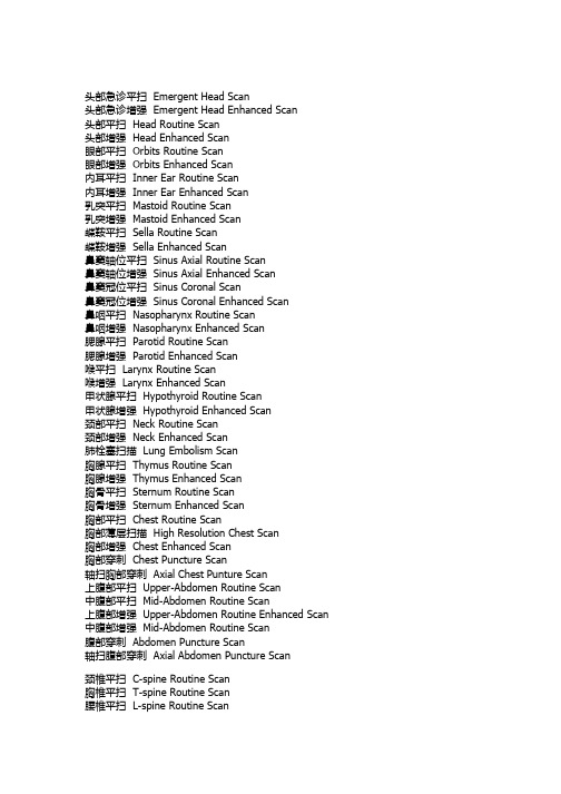
头部急诊平扫 Emergent Head Scan头部急诊增强 Emergent Head Enhanced Scan头部平扫 Head Routine Scan头部增强 Head Enhanced Scan眼部平扫 Orbits Routine Scan眼部增强 Orbits Enhanced Scan内耳平扫 Inner Ear Routine Scan内耳增强 Inner Ear Enhanced Scan乳突平扫 Mastoid Routine Scan乳突增强 Mastoid Enhanced Scan蝶鞍平扫 Sella Routine Scan蝶鞍增强 Sella Enhanced Scan鼻窦轴位平扫 Sinus Axial Routine Scan鼻窦轴位增强 Sinus Axial Enhanced Scan鼻窦冠位平扫 Sinus Coronal Scan鼻窦冠位增强 Sinus Coronal Enhanced Scan鼻咽平扫 Nasopharynx Routine Scan鼻咽增强 Nasopharynx Enhanced Scan腮腺平扫 Parotid Routine Scan腮腺增强 Parotid Enhanced Scan喉平扫 Larynx Routine Scan喉增强 Larynx Enhanced Scan甲状腺平扫 Hypothyroid Routine Scan甲状腺增强 Hypothyroid Enhanced Scan颈部平扫 Neck Routine Scan颈部增强 Neck Enhanced Scan肺栓塞扫描 Lung Embolism Scan胸腺平扫 Thymus Routine Scan胸腺增强 Thymus Enhanced Scan胸骨平扫 Sternum Routine Scan胸骨增强 Sternum Enhanced Scan胸部平扫 Chest Routine Scan胸部薄层扫描 High Resolution Chest Scan胸部增强 Chest Enhanced Scan胸部穿刺 Chest Puncture Scan轴扫胸部穿刺 Axial Chest Punture Scan上腹部平扫 Upper-Abdomen Routine Scan中腹部平扫 Mid-Abdomen Routine Scan上腹部增强 Upper-Abdomen Routine Enhanced Scan 中腹部增强 Mid-Abdomen Routine Scan腹部穿刺 Abdomen Puncture Scan轴扫腹部穿刺 Axial Abdomen Puncture Scan颈椎平扫 C-spine Routine Scan胸椎平扫 T-spine Routine Scan腰椎平扫 L-spine Routine Scan盆腔平扫 Pelvis Routine Scan盆腔增强 Pelvis Enhanced Scan骶髂关节平扫 SI Joint Scan肩关节平扫 Shoulder Joint Scan上肢软组织平扫 Upper Extremities Soft Tissue Scan上肢软组织增强 Upper Extremities Soft Tissue Enhanced 肘关节平扫 Elbow Joint Routine Scan腕关节平扫 Wrist Joint Routine Scan手部平扫 Hand Routine Scan髋关节平扫 Hip Joint Routine Scan膝关节平扫 Knee Joint Routine Scan踝关节平扫 Ankle Joint Routine Scan下肢软组织平扫 Lower Extremities Soft Tissue Scan下肢软组织增强 Lower Extremities Soft Tissue Enhanced 足部平扫 Foot Routine Scan血管造影和三维成像头部血管造影 Head CT Angiography颈部血管造影 Neck CT Angiography心脏冠脉造影 Coronal Artery Angiography心脏冠脉钙化积分 Cardiac Calcium Scoring Scan胸部血管造影 Chest CT Angiography腹部血管造影 Abdomen CT Angiography上肢血管造影 Upper Extremities CT Angiography下肢血管造影 Lower Extremities CT Angiography医界资讯网五官三维成像 3D Facial Scan胃三维 3D Stomach CT Scan结肠三维 3D Colon CT Scan颈椎三维 3D C-Spine胸椎三维 3D T-Spine腰椎三维 3D L-Spine肩关节三维 3D Shoulder Joint肘关节三维 3D Elbow Joint腕关节三维 3D Wrist Joint髋关节三维 3D Hip Joint膝关节三维 3D Knee Joint踝关节三维 3D Ankle Joint检查名称英文对照头部平扫 Head Routine Scan头部常规增强 Head Routine Enhanced Scan头部动态增强 Head Dynamic Enhanced Scan垂体平扫 Sella Routine Scan垂体增强 Sella Enhanced Scan鼻咽部平扫 Nasopharynx Routine Scan鼻咽部增强 Nasopharynx Enhanced Scan眼眶部平扫 Orbits Routine Scan眼眶部增强 Orbits Enhanced Scan内听道平扫 Inner Ear Routine Scan颈部平扫 Neck Routine Scan颈部普通增强 Neck Enhanced Scan颈部动态增强 Neck Dynamic Enhanced Scan上腹部平扫 Upper Abdomen Scan上腹部普通增强 Upper Abdomen Routine Enhanced 上腹部动态增强 Upper Abdomen Dynamic Enhanced 中腹部平扫 Mid-Abdomen Scan中腹部普通增强 Mid-Abdomen Routine Enhanced 中腹部动态增强 Mid-Abdomen Dynamic Enhanced 肾脏平扫 Kidney Routine Scan肾上腺平扫 Adrenal Routine Scan肾脏普通增强 Kidney Routine Enhanced Scan肾脏动态增强 Kidney Dynamic Enhanced Scan胰胆管造影 MRCP尿路造影 MRU腹和盆腔联合扫描 Abdomen & Pelvis Scan医界资讯网颈椎平扫 C-spine Scan颈椎增强 C-spine Enhanced Scan胸椎平扫 T-spine Scan胸椎增强 T-spine Enhanced Scan腰椎平扫 L-spine Scan腰椎增强 L-spine Enhanced Scan胸腰段平扫 T&L Spine Scan胸腰段增强 T&L Spine Enhanced Scan胸部平扫 Chest Scan胸部普通增强 Chest Routine Enhanced Scan胸部动态增强 Chest Dynamic Enhanced Scan女性盆腔平扫 Female Pelvis Scan女性盆腔普通增强 Female Pelvis Routine Enhanced 女性盆腔动态增强 Female Pelvis Dynamic Enhanced 男性盆腔平扫 Male Pelvis Scan男性盆腔普通增强 Male Pelvis Routine Enhanced男性盆腔动态增强 Male Pelvis Dynamic Enhanced 肩关节平扫 Shoulder Joint Scan肘关节平扫 Elbow Joint Scan腕关节平扫 Wrist Joint Scan手部平扫 Hand Scan上肢软组织平扫 Upper Soft Tissue Scan上肢软组织普通增强 Upper Soft Tissue Routine Enhanced 上肢软组织动态增强 Upper Soft Tissue Dynamic Enhanced 骶髂关节平扫 Sacrum Ilium Joint Scan髋关节平扫 Hip Joint Scan膝关节平扫 Knee Joint Routine Scan踝关节平扫 Ankle Joint Routine Scan足部平扫 Foot Routine Scan下肢软组织平扫 Lower Soft Tissue Scan下肢软组织普通增强 Lower Soft Tissue Routine Enhanced 下肢软组织动态增强 Lower Soft Tissue Dynamic Enhanced 头颅正侧位 Skull PA & LAT鼻窦 Sinus PA左侧乳突 Left Mastoid Process医界资讯网右侧乳突 Right Mastoid Process鼻骨侧位 Nasal Bones LAT颈椎正侧位 C-Spine PA & LAT颈椎双斜位 C-Spine Dual Oblique胸椎正侧位 T-Spine PA & LAT腰椎正侧位 L-Spine PA & LAT骶尾正侧位 Saccrum/Coccyx AP & LAT胸部正侧位（成人） Chest PA & LAT (Adult)胸部正侧位（儿童） Chest PA & LAT (Pediatrics)骨盆（成人） Pelvis PA (Adult)骨盆（儿童） Pelvis PA (Pediatrics)腹部（成人） Abdomen ( Adult)腹部（儿童） Abdomen (Pediatircs)左侧肩关节 Left Shoulder Joint右侧肩关节 Right Shoulder Joint左侧肱骨正侧位 Left Humerus AP & LAT右侧肱骨正侧位 Right Humerus AP & LAT左侧尺桡骨正侧位 Left Forearm AP & LAT右侧尺桡骨正侧位 Right Forearm AP & LAT左侧肘关节正侧位 Left Elbow Joint AP & LAT右侧肘关节正侧位 Right Elbow Joint AP & LAT左手正斜位 Left Hand AP & Oblique右手正斜位 Right Hand AP & Oblique左侧腕关节正侧位 Left Wrist Joint AP & LAT右侧腕关节正侧位 Right Wrist Joint AP & LAT双腕关节正位（成人） Dual Wrist Joint AP (Adult)双腕关节正位（儿童） Dual Wrist Joint AP (Pediatrics)左侧股骨正侧位 Left Femur AP & LAT右侧股骨正侧位 Right Femur AP & LAT左侧膝关节正侧位 Left Knee Joint AP & LAT右侧膝关节正侧位 Right Knee Joint AP & LAT左侧胫腓骨正侧位 Left Tibia Fibula AP & LAT右侧胫腓骨正侧位 Right Tibia Fibula AP & LAT左侧踝关节正侧位 Left Ankle Joint AP & LAT右侧踝关节正侧位 Right Ankle Joint AP & LAT左侧足部正侧位 Left Foot AP & LAT右侧足部正侧位 Right Foot AP & LAT足跟侧位 Calcaneus LAT胸部正位 Chest PA胸部正侧位 Chest PA & LAT心脏三位片 Heart胸部斜位 Chest OBL胸骨侧位 Sternum LAT胸锁骨关节像 Sternum Calvicle Joint PA锁骨正位 Calvicle PA肩关节正位 Shoulder Joint AP头颅正位 Skull AP头颅正侧 Skull AP & LAT颈椎正位 C-spine AP颈椎张口位 C-spine Open Mouth颈椎正侧位 C-spine AP & LAT颈椎正侧双斜位 C-spine AP & LAT & Dual OBL颈椎六位像 C-spine 6 position颈椎正侧双斜张口位 C-spine AP & LAT & Dual OBL Open Mouth 颈胸段正侧位 C-T-spine AP & LAT胸椎正侧 T-spine AP & LAT胸腰段正侧位 T-L-spine AP & LAT腰椎正侧位 L-spine AP & LAT腰椎正侧双斜 L-spine AP & LAT & Dual OBL腰椎双斜 L-spine Dual OBL腰椎六位像 L-spine 6 position腰椎过伸过屈位 L-spine Lordotic Kyphotic Position腰骶椎正侧位 L-S-spine AP & LAT骶尾椎正侧位 Saccrum/Coccyx AP & LAT尾椎侧位像 Coccyx LAT骶髂关节正位 Sacrum Ilium Joint AP骶髂关节切线位 Sacrum Ilium Joint Tangential Position骨盆正位 Pelvis AP耻骨坐骨正位 Pubis Ischium AP腹部平片 Abdomen AP上肢 Upper Extremities下肢 Lower Extremities华氏位 Waltz Position下颌骨正侧位 Mandible PA_LAT头颅正侧位 Skull PA_LAT颧弓切线位 Zygomatic小儿胸片 Chest膝关节造影 Knee Joint Contrast肩关节造影 Shoulder Joint Contrast椎管造影 Spinal ContrastTMJ造影 TMJ contrast腮腺造影 Parotid Contrast静脉肾盂造影 IVP逆行尿路造影 Contrary Urethral Contrast子宫造影 Uterus ContrastT管造影 T-tube Cholangiography五官造影 Facial Contrast窦道造影 Contrast Fistulography瘤腔造影 Tumor Cavity Contrast异物定位 Orientation胆系造影 CholecystographyERCP ERCP上消化道造影 Upper Gastrointestinal Contrast全消化道造影 Full Gastrointestinal Contrast钡灌肠造影 Barium Contrast of Colon小肠低张造影 Small Bowel Enema结肠低张造影 Hypotonic Colon Contrast食道造影 Contrast Esophagography下肢静脉造影 Lower Vein Angiography上肢静脉造影 Upper Vein Angiography下肢动脉造影 Lower Artery Angiography上肢动脉造影 Upper Artery Angiography脑血管造影 Cerebrovascular Angiograhy主动脉弓胸腹主动脉造影 Aorta Angiography肾静脉取血 Kidney Vein Blood Sampling右心、左心造影 Right and Left Ventricular Angiography 心肌活检 Myocardiam Centesis and Sampling冠状动脉造影 Coronary Arteriography腔静脉取血 Vena cava sampling心导管检查(微导管同)(进口仪器） Cardiac catheterization经皮球囊扩张 Percutaneous balloon dilatating予激综合症心内膜检测 Endocardial investigation of preexcitation syndrome希氏束电图 Electrocardiogram of bundle of His心脏临时起搏 Cardiac temporary pacing埋置永久心脏起搏器 Cardioc permanent pacemaker implanting体肢动脉系统介入治疗 Transartery interventional therapy支气管动脉介入治疗 Bronchus artery interventional therapy肺动脉介入治疗 Pulmonary artery interventional therapy头臂动脉介入治疗 Brachiocephalic artery interventional therapy静脉介入治疗 Veinous interventional therapy冠状动脉介入治疗(球囊成形) Coronary Artery interventional therapy (balloon angioplasty)冠状动脉介入治疗(腔内旋磨) Coronary Artery interventional therapy (rotablating)冠状动脉介入治疗(腔内支架) Coronary Artery interventional therapy (stent implantaion)主动脉介入治疗 Aorta interventional therapy肾动脉介入治疗 Renal artery interventional therapy心脏瓣膜成形术 Heart valvuloplasty房间隔缺损封堵术 Atrial septal defect closer室间隔缺损封堵术 Ventricular septal defect closer动脉导管封堵术 Patent doctus arteriosus closer冠状动脉瘘封堵术 Coronary artery fistula closer冠状动脉腔内超声 Intracoronary ultrasound非冠状动脉血管内支架置入治疗 Stenting therapy of non-coronary artery经皮清除血管内异物 Transluminal eyewinker clearing经皮放置静脉滤器 Transluminal filter implantaion上肢MRA Upper Extremities MRA下肢MRA Lower Extremities MRA心脏大血管造影 Heart MR Angiography胸主动脉造影 T-Artery MR Angiography腹主动脉造影 Abd-Artery MR Angiography头部血管造影 Head MR Angiography颈部血管造影 Head MR Angiography盆腔血管造影 Pelvis MR Angiography。

(医学影像学)中英文对照学生翻译版

团队的力量 Strength of our team！湘雅医院2008级五年制临床医学、麻醉医学及口腔七年制18组同学合作完成本文的翻译Double-Contrast Upper Gastrointestinal Radiography: A Pattern Approach for Diseases of the StomachAbstractThe double-contrast upper gastrointestinal series is a valuable diagnostic test for evaluating structural and functional abnormalities of the stomach. This article will review the normal radiographic anatomy of the stomach. The principles of analyzing double-contrast images will be discussed. A pattern approach for the diagnosis of gastric abnormalities will also be presented, focusing on abnormal mucosal patterns, depressed lesions, protruded lesions, thickened folds, and gastric narrowing.This article presents a pattern approach for the diagnosis of diseases of the stomach at double-contrast upper gastrointestinal radiography. After describing the normal appearance of the stomach on double-contrast barium studies and the principles ofdouble-contrast image interpretation, we will consider abnormal surface patterns of the mucosa, depressed lesions (erosions and ulcers), protruded lesions (polyps, submucosal masses, and other tumors), thickened folds, and gastric narrowing. 上消化道双重对比造影：一种用于胃部疾病诊断的成像方法摘要上消化道双重对比造影系列是用于评估胃部结构性和功能性病变的一种极有价值的诊断方法。

图像处理中英文对照外文翻译文献

中英文对照外文翻译文献(文档含英文原文和中文翻译)译文：基于局部二值模式多分辨率的灰度和旋转不变性的纹理分类摘要：本文描述了理论上非常简单但非常有效的，基于局部二值模式的、样图的非参数识别和原型分类的，多分辨率的灰度和旋转不变性的纹理分类方法。

此方法是基于结合某种均衡局部二值模式，是局部图像纹理的基本特性，并且已经证明生成的直方图是非常有效的纹理特征。

我们获得一个一般灰度和旋转不变的算子，可表达检测有角空间和空间结构的任意量子化的均衡模式，并提出了结合多种算子的多分辨率分析方法。

根据定义，该算子在图像灰度发生单一变化时具有不变性，所以所提出的方法在灰度发生变化时是非常强健的。

另一个优点是计算简单，算子在小邻域内或同一查找表内只要几个操作就可实现。

在旋转不变性的实际问题中得到了良好的实验结果,与来自其他的旋转角度的样品一起以一个特别的旋转角度试验而且测试得到分类, 证明了基于简单旋转的发生统计学的不变性二值模式的分辨是可以达成。

这些算子表示局部图像纹理的空间结构的又一特色是，由结合所表示的局部图像纹理的差别的旋转不变量不一致方法，其性能可得到进一步的改良。

这些直角的措施共同证明了这是旋转不变性纹理分析的非常有力的工具。

关键词：非参数的，纹理分析，Outex ，Brodatz ，分类，直方图，对比度2 灰度和旋转不变性的局部二值模式我们通过定义单色纹理图像的一个局部邻域的纹理T ，如 P （P>1）个象素点的灰度级联合分布，来描述灰度和旋转不变性算子：01(,,)c P T t g g g -= （1）其中，g c 为局部邻域中心像素点的灰度值，g p （p=0，1…P-1）为半径R(R>0)的圆形邻域内对称的空间象素点集的灰度值。

图1如果g c 的坐标是（0,0），那么g p 的坐标为(cos sin(2/),(2/))R R p P p P ππ-。

图1举例说明了圆形对称邻域集内各种不同的（P,R ）。

图像的分割和配准中英文翻译

外文文献资料翻译：李睿钦指导老师：刘文军Medical image registration with partial dataSenthil Periaswamy，Hany FaridThe goal of image registration is to find a transformation that aligns one image to another. Medical image registration has emerged from this broad area of research as a particularly active field. This activity is due in part to the many clinical applications including diagnosis, longitudinal studies, and surgical planning, and to the need for registration across different imaging modalities (e.g., MRI, CT, PET, X-ray, etc.). Medical image registration, however, still presents many challenges. Several notable difficulties are (1) the transformation between images can vary widely and be highly non-rigid in nature; (2) images acquired from different modalities may differ significantly in overall appearance and resolution; (3) there may not be a one-to-one correspondence between the images (missing/partial data); and (4) each imaging modality introduces its own unique challenges, making it difficult to develop a single generic registration algorithm.In estimating the transformation that aligns two images we must choose: (1) to estimate the transformation between a small number of extracted features, or between the complete unprocessed intensity images; (2) a model that describes the geometric transformation; (3) whether to and how to explicitly model intensity changes; (4) an error metric that incorporates the previous three choices; and (5) a minimization technique for minimizing the error metric, yielding the desired transformation.Feature-based approaches extract a (typically small) number of corresponding landmarks or features between the pair of images to be registered. The overall transformation is estimated from these features. Common features include corresponding points, edges, contours or surfaces. These features may be specified manually or extracted automatically. Fiducial markers may also be used as features;these markers are usually selected to be visible in different modalities. Feature-based approaches have the advantage of greatly reducing computational complexity. Depending on the feature extraction process, these approaches may also be more robust to intensity variations that arise during, for example, cross modality registration. Also, features may be chosen to help reduce sensor noise. These approaches can be, however, highly sensitive to the accuracy of the feature extraction. Intensity-based approaches, on the other hand, estimate the transformation between the entire intensity images. Such an approach is typically more computationally demanding, but avoids the difficulties of a feature extraction stage.Independent of the choice of a feature- or intensity-based technique, a model describing the geometric transform is required. A common and straightforward choice is a model that embodies a single global transformation. The problem of estimating a global translation and rotation parameter has been studied in detail, and a closed form solution was proposed by Schonemann. Other closed-form solutions include methods based on singular value decomposition (SVD), eigenvalue-eigenvector decomposition and unit quaternions. One idea for a global transformation model is to use polynomials. For example, a zeroth-order polynomial limits the transformation to simple translations, a first-order polynomial allows for an affine transformation, and, of course, higher-order polynomials can be employed yielding progressively more flexible transformations. For example, the registration package Automated Image Registration (AIR) can employ (as an option) a fifth-order polynomial consisting of 168 parameters (for 3-D registration). The global approach has the advantage that the model consists of a relatively small number of parameters to be estimated, and the global nature of the model ensures a consistent transformation across the entire image. The disadvantage of this approach is that estimation of higher-order polynomials can lead to an unstable transformation, especially near the image boundaries. In addition, a relatively small and local perturbation can cause disproportionate and unpredictable changes in the overall transformation. An alternative to these global approaches are techniques that model the global transformation as a piecewise collection of local transformations. For example, the transformation between each local region may bemodeled with a low-order polynomial, and global consistency is enforced via some form of a smoothness constraint. The advantage of such an approach is that it is capable of modeling highly nonlinear transformations without the numerical instability of high-order global models. The disadvantage is one of computational inefficiency due to the significantly larger number of model parameters that need to be estimated, and the need to guarantee global consistency. Low-order polynomials are, of course, only one of many possible local models that may be employed. Other local models include B-splines, thin-plate splines, and a multitude of related techniques. The package Statistical Parametric Mapping (SPM) uses the low-frequency discrete cosine basis functions, where a bending-energy function is used to ensure global consistency. Physics-based techniques that compute a local geometric transform include those based on the Navier–Stokes equilibrium equations for linear elastici and those based on viscous fluid approaches.Under certain conditions a purely geometric transformation is sufficient to model the transformation between a pair of images. Under many real-world conditions, however, the images undergo changes in both geometry and intensity (e.g., brightness and contrast). Many registration techniques attempt to remove these intensity differences with a pre-processing stage, such as histogram matching or homomorphic filtering. The issues involved with modeling intensity differences are similar to those involved in choosing a geometric model. Because the simultaneous estimation of geometric and intensity changes can be difficult, few techniques build explicit models of intensity differences. A few notable exceptions include AIR, in which global intensity differences are modeled with a single multiplicative contrast term, and SPM in which local intensity differences are modeled with a basis function approach.Having decided upon a transformation model, the task of estimating the model parameters begins. As a first step, an error function in the model parameters must be chosen. This error function should embody some notion of what is meant for a pair of images to be registered. Perhaps the most common choice is a mean square error (MSE), defined as the mean of the square of the differences (in either feature distance or intensity) between the pair of images. This metric is easy to compute and oftenaffords simple minimization techniques. A variation of this metric is the unnormalized correlation coefficient applicable to intensity-based techniques. This error metric is defined as the sum of the point-wise products of the image intensities, and can be efficiently computed using Fourier techniques. A disadvantage of these error metrics is that images that would qualitatively be considered to be in good registration may still have large errors due to, for example, intensity variations, or slight misalignments. Another error metric (included in AIR) is the ratio of image uniformity (RIU) defined as the normalized standard deviation of the ratio of image intensities. Such a metric is invariant to overall intensity scale differences, but typically leads to nonlinear minimization schemes. Mutual information, entropy and the Pearson product moment cross correlation are just a few examples of other possible error functions. Such error metrics are often adopted to deal with the lack of an explicit model of intensity transformations .In the final step of registration, the chosen error function is minimized yielding the desired model parameters. In the most straightforward case, least-squares estimation is used when the error function is linear in the unknown model parameters. This closed-form solution is attractive as it avoids the pitfalls of iterative minimization schemes such as gradient-descent or simulated annealing. Such nonlinear minimization schemes are, however, necessary due to an often nonlinear error function. A reasonable compromise between these approaches is to begin with a linear error function, solve using least-squares, and use this solution as a starting point for a nonlinear minimization.译文：部分信息的医学图像配准Senthil Periaswamy，Hany Farid图像配准的目的是找到一种能把一副图像对准另外一副图像的变换算法。

医学影像学外文文献翻译、中英文翻译

医学影像学外文文献翻译、中英文翻译本文旨在翻译医学影像学相关的外文文献，并提供中英文对照。

以下是翻译文档的内容。

文献一标题：脑神经影响因素对医学影像学的影响原文摘要：本文研究了脑神经对医学影像学的影响因素。

通过对多个神经病例进行分析，发现脑神经异常会导致医学影像学结果的变异。

这一发现揭示了脑神经对医学影像学的重要性。

翻译摘要：This article investigates the influence of cranial nerves on medical imaging. By analyzing multiple neurological cases, it is found that abnormalities in cranial nerves can cause variationsin medical imaging results. This finding highlights the importance of cranial nerves in medical imaging.文献二标题：放射性示踪剂在医学影像学中的应用原文摘要：本文综述了放射性示踪剂在医学影像学中的应用。

通过注射放射性示踪剂，医生可以通过影像学方法观察其在患者体内的分布情况，从而得出诊断结果。

放射性示踪剂在医学影像学中起到了重要的作用。

翻译摘要：This article reviews the application of radiopharmaceuticals in medical imaging. By injecting radiopharmaceuticals, doctors can observe their distribution in the patient's body using imaging techniques to obtain diagnostic results. Radiopharmaceuticals play a crucial role in medical imaging.以上是医学影像学相关外文文献的翻译和中英文对照。

图像融合技术中英文对照外文翻译文献

中英文资料对照外文翻译使用不变特征的全景图像自动拼接摘要本文研究全自动全景图像的拼接问题，尽管一维问题（单一旋转轴）很好研究，但二维或多行拼接却比较困难。

以前的方法使用人工输入或限制图像序列，以建立匹配的图像，在这篇文章中，我们假定拼接是一个多图像匹配问题，并使用不变的局部特征来找到所有图像的匹配特征。

由于以上这些，该方法对输入图像的顺序、方向、尺度和亮度变化都不敏感；它也对不属于全景图一部分的噪声图像不敏感，并可以在一个无序的图像数据集中识别多个全景图。

此外，为了提供更多有关的细节，本文通过引入增益补偿和自动校直步骤延伸了我们以前在该领域的工作。

1. 简介全景图像拼接已经有了大量的研究文献和一些商业应用。

这个问题的基本几何学很好理解，对于每个图像由一个估计的3×3的摄像机矩阵或对应矩阵组成。

估计处理通常由用户输入近似的校直图像或者一个固定的图像序列来初始化，例如，佳能数码相机内的图像拼接软件需要水平或垂直扫描，或图像的方阵。

在自动定位进行前，第4版的REALVIZ拼接软件有一个用户界面，用鼠标在图像大致定位，而我们的研究是有新意的，因为不需要提供这样的初始化。

根据研究文献，图像自动对齐和拼接的方法大致可分为两类——直接的和基于特征的。

直接的方法有这样的优点，它们使用所有可利用的图像数据，因此可以提供非常准确的定位，但是需要一个只有细微差别的初始化处理。

基于特征的配准不需要初始化，但是缺少不变性的传统的特征匹配方法（例如，Harris角点图像修补的相关性）需要实现任意全景图像序列的可靠匹配。

在本文中，我们描述了一个基于不变特征的方法实现全自动全景图像的拼接，相比以前的方法有以下几个优点。

第一，不变特征的使用实现全景图像序列的可靠匹配，尽管在输入图像中有旋转、缩放和光照变化。

第二，通过假定图像拼接是一个多图像匹配问题，我们可以自动发现这些图像间的匹配关系，并且在无序的数据集中识别出全景图。

医学图谱和图像的中英文译名整理

医学图谱和图像的中英文译名整理在医学领域，图谱和图像等术语的准确译名对于学术交流和专业研究至关重要。

本文将针对医学图谱和图像的中英文译名进行整理和解释。

一、图谱的英文译名1. 图谱(tú pǔ)图谱是指将某一特定领域或知识体系以图形形式进行展示的结果。

学术上常用的图谱包括知识图谱、基因组图谱等。

在英文中，图谱可以翻译为"chart"、"map"或"diagram"等。

2. 知识图谱(zhī shí tú pǔ)知识图谱是指将人类知识以图形化的方式进行展示的一种工具。

它通过对知识的梳理和整理，将知识元素和其之间的关系进行可视化。

在英文中，知识图谱可以翻译为"knowledge graph"。

3. 基因组图谱(jī yīn zǔ tú pǔ)基因组图谱是指对某个物种的基因组进行测序和解读后，将其基因信息以图形化的方式展示的结果。

在英文中，基因组图谱可以翻译为"genome map"。

二、图像的英文译名1. 图像 (tú xiàng)图像是指由光线、电磁波等产生的在人眼或摄像机等器官中形成的视觉表现。

图像可以是实物的照片、绘画，也可以是数字形式的图片、视频等。

在英文中，图像可以翻译为"image"。

2. 医学影像(yī xué yǐng xiàng)医学影像是指应用医学成像技术所获得的关于人体内部结构、功能和病变的图像。

常见的医学影像包括X光片、CT扫描、MRI等。

在英文中，医学影像可以翻译为"medical imaging"或"medical image"。

3. 数字图像 (shù zì tú xiàng)数字图像是指以数字形式存储和表示的图像。

医学影像技术的发展论文中英文对照资料外文翻译文献

医学影像技术的发展论文中英文对照资料外文翻译文献随着科技的不断进步，医学影像技术也在不断地更新与发展。

医学影像技术包括许多技术和设备，如X光、CT、MRI、PET、超声波和电子显微镜等。

这些技术和设备已经成为现代医药领域的重要工具。

医学影像技术的引入和发展改变了医疗诊断和治疗的方式，提高了医疗服务的效率和质量，并有助于减少医学风险。

近年来，人工智能技术在医学影像技术中的应用也越来越广泛。

医学影像技术与人工智能技术的结合有助于提高医疗服务的质量和效率。

例如，人工智能技术可以帮助医生快速识别医学影像中的异常情况，从而更快地制定治疗方案。

此外，人工智能技术还可以帮助医生决定哪些患者需要进行进一步的检查和测试。

总之，医学影像技术的发展和人工智能技术的应用为医疗行业带来了很大的变化和进步。

未来，医学影像技术和人工智能技术的发展将继续为人类健康服务做出更多的贡献。

In conclusion, the development of medical imaging technology and the application of artificial intelligence technology have brought about great changes and progress for the medical industry. In the future, the development of medical imaging technology and artificial intelligence technology will continue to make more contributions to human health services.。

医疗影像分析的深度学习模型研究(英文中文双语版优质文档)

医疗影像分析的深度学习模型研究（英文中文双语版优质文档）With the continuous development of medical technology, medical imaging is more and more widely used in clinical practice. However, the analysis and diagnosis of medical images usually takes a lot of time and manpower, and the accuracy is also affected by the doctor's personal experience. In recent years, the emergence of deep learning technology has brought new opportunities and challenges for medical image analysis. This article will deeply discuss the research on deep learning models for medical image analysis, including the application and research progress of models such as convolutional neural network (CNN), recurrent neural network (RNN) and generative adversarial network (GAN).1. Application of convolutional neural network (CNN) model in medical image analysisConvolutional neural network is a state-of-the-art deep learning model, which has a wide range of applications in the field of medical image analysis. Convolutional neural networks can automatically extract features from medical images and classify them as normal and abnormal. For example, in medical image analysis, convolutional neural networks can be used to analyze lung X-rays to identify lung diseases such as pneumonia, tuberculosis, and lung cancer. In addition, convolutional neural networks can also be used for segmentation and registration of medical images for more precise localization and identification of lesions.2. Application of Recurrent Neural Network (RNN) Model in Medical Image AnalysisA recurrent neural network is a deep learning model capable of processing sequential data. In medical image analysis, recurrent neural networks are often used to analyze time series data, such as electrocardiograms and electroencephalograms in medical images. The cyclic neural network can automatically extract the features in the time series data, so as to realize the classification and recognition of medical images. For example, in the diagnosis of heart disease, a recurrent neural network can identify heart diseases such as arrhythmia and myocardial infarction by analyzing ECG data.3. Application of Generative Adversarial Network (GAN) Model in Medical Image AnalysisGenerative adversarial networks, a deep learning model capable of generating realistic images, have also been widely used in medical image analysis in recent years. Generative adversarial networks usually consist of two neural networks, one is a generative network, which is responsible for generating realistic images; the other is a discriminative network, which is used to judge whether the images generated by the generative network are consistent with real images. In medical image analysis, GAN can be used to generate realistic medical images, such as MRI images, CT images, etc., to help doctors better diagnose and treat. In addition, the generative confrontation network can also be used for denoising and enhancement of medical images to improve the clarity and accuracy of medical images.In conclusion, the application of deep learning models in medical image analysis has broad prospects and challenges. With the continuous development of technology and the deepening of research, the application of deep learning models in medical image analysis will become more and more extensive and in-depth, making greater contributions to the progress and development of clinical medicine.随着医疗技术的不断发展，医疗影像在临床中的应用越来越广泛。

1、下载文档前请自行甄别文档内容的完整性，平台不提供额外的编辑、内容补充、找答案等附加服务。
2、"仅部分预览"的文档,不可在线预览部分如存在完整性等问题,可反馈申请退款(可完整预览的文档不适用该条件!)。
3、如文档侵犯您的权益，请联系客服反馈,我们会尽快为您处理(人工客服工作时间：9:00-18:30)。

中英文对照外文翻译文献(文档含英文原文和中文翻译)译文：一种图像拼接和融合摘要在许多临床研究，包括癌症，这是非常可取的，以获取图像的整个肿瘤节同时保留一个微小的决议。

通常的办法是建立一个综合的形象，适当重叠个人获得的图象在高倍显微镜下。

一块镶嵌图，这些图片可以准确地运用所形成的图像配准，重复搬运和混合技术。

我们描述的最优化，自动，快速和可靠的方法，既形象加入和融合。

这些算法可以适用于大多数类型的光学显微镜的成像。

从组织学，从体内血管成像和荧光等方面的应用表明，无论是在二维和三维。

算法的不同形象重叠的阶段有所不同，但例子综合获得的图象既手动驱动，电脑控制的阶段介绍。

重叠迁移算法是基于互相关的方法，这是用来确定和选择最佳的相关点之间的任何新的形象和以前的综合形象。

补充图片混合算法的基础上，梯度法，是用来消除强度变化急剧的形象加入，从而逐渐融合到一个图像邻近'复合'的细节，该算法克服强度差异和几何失调图像之间的缝合将介绍和说明了几个例子。

关键词：图像拼接，共混，镶嵌图像1 。

导言和背景有许多应用需要高分辨率图像。

在明亮的场或落射荧光显微镜[ 1 ] ，例如，用于生物和医学应用中，通常需要分析一个完整的组织部分已层面几十毫米，在高分辨率。

然而，高分辨率单图片不能意识到了低功耗的目标，必要的，以查看大样本，即使使用数码相机时的几万数以百万计的积极像素。

最常见的方法是获得一些图片的部分组织在高放大率和组装成一个复合单一形象保持高分辨率。

这一过程的组装复合图像从一些图片，也被称为'块'或'拼图'需要一个算法为图像拼接（登记）和混合。

自动建立大型高分辨率图像的马赛克是一种越来越多的研究领域涉及计算机视觉和图像处理。

拼接与融合可以被界定为生产单一edgeless形象整理一套重叠图像[ 2 ] 。

自动化这一进程是一个重要的问题，因为它是困难和消耗时间，以实现手动。

这样的一个算法的图像拼接和融合是本文介绍了。

图像拼接结合了一些拍摄高分辨率纳入一个综合的形象。

综合图像必须包括图像放在正确的位置和目标是使图像边缘之间的无形的。

那个质量表示缝合因此通过测量两个相邻的信件图像缝合形成了综合形象和知名度煤层之间的缝合图像[ 3 ] 。

图像拼接（注册）方法已详细解释[ 4 ] 。

[ 5 ]中，互相关证明是最好的方法，自动注册大量的图像。

各种登记方法进行了比较研究[ 5 ]这是显示的互相关法提供了最小的错误。

当这些方法进行了比较而言，速度，交叉相关证明是第二快的，但更准确比速度最快的方法（主轴法）。

有一些文件，处理问题的缝合[ 3 ， 6-8 ] 。

图像拼接可以用图像像素直接-相关法，在频域-快速傅里叶变换法;利用水平低功能，如棱角;使用高层次的功能，如部分对象[ 2 ] 。

布朗[ 4 ]分类图片登记根据以下标准：类型的功能空间，类型的搜索策略和类型的相似性措施。

图像拼接方法的优化，寻求最佳的相关点使用以Levenberg - Marquardt 方法给出了[ 2 ， 9 ， 10 ] 。

以Levenberg - Marquardt方法使良好的效果，但它是昂贵和计算能停留在局部极小。

还有一种方法是运用一个算法搜索最佳的相关点拥有由'粗到细的决议的办法，以减少计算[ 10 ， 11 ] 。

该方法提供了本文所选择的最佳关联点，以下列方式。

基于了解预期重叠当使用机动阶段，这将是直截了当的，以找到最佳的相关点在理想的情况。

然而，重叠面积并非尽善尽美，而且肯定不是一个准确的一像素，由于偏离阶段的理想位置，而且由于舞台/相机失调。

我们的算法提供了一个如何克服这一问题，寻找周围地区的小预期中央重叠像素，以便找到最佳关联点。

定位获得图像手册阶段小得多准确，因此有必要寻找更广阔的领域，以找到最佳的关联点。

大多数现有方法的图像拼接或者制作一个粗略'缝，不能处理的共同特征如血管，彗星细胞和组织，或者他们需要一些用户输入[ 12 ] 。

新算法的提出本文介绍了嵌入式代码来处理这种功能。

为了消除边缘，使一个紧凑的形象，有必要适用于更多的图像融合。

那个图像融合过程中限制区的重叠这是确定在缝合过程。

这个也就是说，如果重叠区域图像间大，图像不完全匹配的这些部分，鬼影或'模糊'是可见的。

但是，如果这些地区的小国，接缝将会看到[ 13 ] 。

为了避免这些影响，使模糊效果微乎其微，在互相关函数之间的综合形象和的形象是被缝合需要适当运用。

新的方法本文介绍表明，最好的质量，才能实现图像融合的应用，如果每张图片后，已缝合。

这种办法提高缝合更多图像，因为互相关应用到混合复合形象，给出了更有力的结果。

当获取图像的高度非均匀样品，因为这是在我们的情况在体内研究中，照明条件变化，从而影响互相关期间适用缝合。

这些照明变化防止取消文物。

为了避免这种影响有可能正常化照明的图像，但它可能会导致有些损失的信息作为一个无法确定的真正原因是什么的变化图像照明。

它可以来自改变照明，而且还从不同的组织的颜色。

因此，一些光照补偿是必要的。

我们的成就是一个高质量，自动拼接和融合算法，响应的功能，如血船只，彗星细胞和组织样本。

光照补偿不纳入提交算法。

本文主办如下。

第2节解释了图像采集过程。

第3节解释采用的方法开发过程中的图像处理算法，该算法适用于缝合和混合。

第4节给出的结果，应用算法选取的图像拼接后只有后两个缝纫和混合，并说明了算法的有效性。

结论中提出的第5款，并指示今后工作的定义。

2 。

图像采集二维图像所有图片被收购，利用标准的显微镜。

所有2D图像获得的样本翻译和收集的手动或自动使用机动阶段。

三种类型的二维图像进行收购。

这些包括图像，组织学，荧光细胞的一个组成部分彗星阵列（彗星细胞），并在体内的血管。

那个安装规范，这些图像是摘要列于表1 。

CCD相机用于获取图像要么一个IEEE 1394接口，或使用一个PCI图像采集（类型：由美国国家仪器公司，英国）。

成像面积的命令1x1平方毫米时，用客观x10 。

CCD相机推出两款噪音影响。

一个是暗电流和另一个是一个非均匀像素反应。

为了取消了暗电流的影响，获得的图象，没有轻被减去图像的样本。

取消的非均匀像素反应，形象的样本除以一个空白图像收购标准照明清洁幻灯片。

镜头畸变也存在。

全部成像系统，由于这种像差，遭受了或多或少从每桶或枕形失真，或他们的组合。

最困难的条件下的图像拼接是那些各种各样的环境照明即强度跨度-空间不同的照明。

据推测，旋转和缩放保持不变全国各地的实验和处理图像。

只有翻译错误必须纠正在缝合过程。

三维图像用于购置三维图像下面的安装使用。

尼康电子200荧光显微镜的使用修改阶段，以适应啮齿动物。

我们在体内的血管图像获得一个窗口商会安排。

它包括双面铝框举行两个平行的玻璃窗。

它位于中央上述的目标[ 14 ] 。

肿瘤血管生成和血管对治疗的反应在这两个形态的血血管网络的功能和个人进行了调查船只使用窗口厅。

多光子显微技术已应用到获取三维图像的肿瘤血管[ 15 ] ，因为这些技术证明是十分有效地获得三维生物的图片。

多光子显微镜系统是基于酶标仪湄公河委员会1024MP工作站，由一个固体statepumped （ 10W的年十， Nd ： YVO4晶体，光谱物理），自锁模钛：蓝宝石（海啸，光谱物理）激光系统，一个中心扫描头，焦探测器和一个倒置显微镜（尼康TE200 ） [ 15 ] 。

多光子显微镜可以准确地找到一个三维荧光量，可成功地应用于分析血管形态。

通常是一个小肿瘤（直径几毫米）植入皮肤的窗口中庭。

整个肿瘤血管的影像大多数实验。

图片10倍的目标而采取的一切，但最小的肿瘤和图像覆盖约1.3x1.3毫米的组织。

成堆的图像所采取的一个典型的堆栈50片。

它通常需要13分钟获得的图像为整个堆栈3 。

图像处理-方法主要有两个阶段在处理这些图像：1 ）图像拼接拼接是由滑动的新形象的综合形象和寻找最佳关联点。

2 ）图像融合配煤是由分离颜色的飞机，在必要情况下，采用混合算法每个彩色带重组飞机一起获得全彩色图像的输出。

混合图像应保持质量输入图像[ 16 ] 。

这些过程中有详细的解释，并参阅下文二维图像，除非明确指出，他们提到的三维图像。

算法开发了C编程语言LabWindows / CVI的7.0 （美国国家仪器有限公司）开发环境，使用IMAQ图像处理图书馆和Windows XP专业版操作系统。

那个算法是完全自动的，他们已经在电脑上测试的处理器速度1.53GHz和448MB的内存。

3.1拼接方法在该算法的缝合是由图像翻译只。

应用程序可以被称为作为拼接，瓦工，montaging或缝合。

第一步是生成的相对位置所获得的图像和建立一个空的图像阵列在电脑记忆体，这些图片将放在。

下一步是搜索对于这一点的最佳关联是由相邻的图像边缘滑动是双向的，直到最佳比赛的边缘特征发现。

这个搜索过程需要选择最佳的搜索空间如图1所示，在其中进行搜索的最佳关联。

使用太多像素内使这个方块相关过程耗时太少像素，同时减少比赛的质量。

选择若干像素使用密切相关的各个方面的功能预期将显着的形象而这又取决于重点质量，即对目前的最大空间频率的形象。

原文：An algorithm for image stitching and blendingABSTRACTIn many clinical studies, including those of cancer, it is highly desirable to acquire images of whole tumour sectionswhilst retaining a microscopic resolution. A usual approach to this is to create a composite image by appropriatelyoverlapping individual images acquired at high magnification under a microscope. A mosaic of these images can beaccurately formed by applying image registration, overlap removal and blending techniques. We describe an optimised,automated, fast and reliable method for both image joining and blending. These algorithms can be applied to most typesof light microscopy imaging. Examples from histology, from in vivo vascular imaging and from fluorescenceapplications are shown, both in 2D and 3D. The algorithms are robust to the varying image overlap of a manually moved stage, though examples of composite images acquired both with manually-driven and computer-controlled stages are presented. The overlap-removal algorithm is based on the cross-correlation method; this is used to determine and select the best correlation point between any new image and the previous composite image. A complementary image blending algorithm, based on a gradient method, is used to eliminate sharp intensity changes at the image joins, thus gradually blending one image onto the adjacent ‘composite’. The details of the algorithm to overcome both intensity discrepancies and geometric misalignments between the stitched images will be presented and illustrated with several examples.Keywords: Image Stitching, Blending, Mosaic images1. INTRODUCTION AND BACKGROUNDThere are many applications which require high resolution images. In bright-field or epifluorescence microscopy [1],for example, which are used in biological and medical applications, it is often necessary to analysea complete tissue section which has dimensions of several tens of millimetres, at high resolution. However, the high resolution single image cannot be realised with a low power objective, necessary to view a large sample, even if using cameras with tens of millions of active pixels. The most common approach is to acquire several images of parts of the tissue at high magnification and assemble them into a composite single image which preserves the high resolution. This process of assembling the composite image from a number of images, also known as ‘tiling’ or ‘mosaicing’ requires an algorithm for image stitching (registration) and blending. The automatic creation of large high resolution image mosaics is a growing research area involving computer vision and image processing. Mosaicing with blending can be defined as producing a single edgeless image by putting together a set of overlapped images [2]. Automating this process is an important issue as it is difficult and time consuming to achieve it manually. One such algorithm for image stitching and blending is presented in this paper. Image stitching combines a number of images taken at high resolution into a composite image. The composite image must consist of images placed at the right position and the aim is to make the edges between images invisible. The quality of stitching is therefore expressed by measuring both the correspondence between adjacent stitched images that form the composite image and the visibility of the seam between the stitched images [3]. Image stitching (registration) methods have been explained in detail in [4]. In [5], cross-correlation is shown to be the preferred method for automatic registration of large number of images. Various registration methods were compared in this paper [5] and it was showed that the cross-correlation method provided the smallest error. When these methods were compared in terms of speed, the cross-correlation was shown to be the second fastest but much more accurate than the fastest method (principal axes method). There are a number of papers that deal with the stitching problem [3, 6-8]. Image stitching can be performed using image pixels directly - correlation method;in frequency domain - fast Fourier transform method; using low level Three-Dimensional and Multidimensional Microscopy: Image Acquisition and Processing XII, Jose-Angel Conchello, Carol J. Cogswell, Tony Wilson, Editors, March 2005 191 features such as edges and corners; using high level features such as parts of objects [2]. Brown [4] classifies image registration according to following criteria: type of feature space, type of search strategies and type of similarity measure.Approaches for image stitching that optimise the search for the best correlation point by using Levenberg-Marquardt method are given in [2, 9, 10]. Levenberg-Marquardt method gives good results, but it is computationally expensive and can get stuck at local minima. An alternative way is to apply an algorithm which searches for the best correlation point by employing a ‘coarse to fine’ resolution approach in order to reduce the number of calculations [10, 11]. The approach offered in this paper makes the selection of the best correlation point in the following way. Based on knowledge about the expected overlap when using the motorised stage, it would be straightforward to find the best correlation point in the ideal case. However, the overlap area is not perfect, and certainly not to an accuracy of one pixel, due to deviations in stage position from the ideal and due to stage/camera misalignment. Our algorithm offers away to overcome this problem by searching the small area around the expected central overlap pixel in order to find the best correlation point. Positioning of acquired images with a manual stage is much less accurate, so there is a need to search a wider area in order to find the best cross-correlation point. Most of the existing methods of image stitching either produce a ‘rough’ stitch that cannot deal with common features such as blood vessels, comet cells and histology, or they require some user input [12]. The new algorithm presented in this paper has embedded code to deal with such features. In order to remove the edges and make one compact image it is necessary to apply additional image blending. The process of image blending is restricted to zones of overlap which aredetermined during the stitching process. This means that if the overlap regions between images are large, and images are not perfectly matched on these parts, ghosting or ‘blurring’ is visible. However, if these regions are small, the seams will be visible [13]. In order to avoid these effects and make the blurring effect negligible, the cross-correlation function between the composite image and the image which is to be stitched needs to be applied appropriately. The new method presented in this paper shows that the best quality image can be achieved if blending is applied after each image has been stitched. This approach improves the stitching of additional images because the cross-correlation is applied to a blended composite image which gives a more robust result. When acquiring images of highly non-uniform samples, as it is the case in our in vivo studies, the lighting conditions change and thus influence the cross-correlation applied during stitching. These lighting changes prevent the removal of artefacts. In order to avoid this effect it may be possible to normalise the illumination of the images, but it could cause some loss of information as one cannot be sure what the real cause for the variation in the image illumination is. It can come from the changes in the lighting but also from the different tissue colour. Hence, some illumination compensation is necessary. Our achievement is ahigh-quality, automatic stitching and blending algorithm that responds to features such as blood vessels, comet cells and histology samples. The illumination compensation is not incorporated in the presented algorithm. This paper is organised as follows. Section 2 explains the image acquisition process. Section 3 explains the methodology followed during the development of the image processing algorithm that applies both the stitching and blending. Section 4 gives the results of the applied algorithm on the selected images after the stitching only and after both stitching and blending and illustrates the effectiveness of the proposed algorithm. Conclusions are presented in Section 5 and directions for the future work are defined.2. IMAGE ACQUISITION2D imagesAll images were acquired using a standard microscope. All 2D images were acquired by sample translation and collected either manually or automatically using the motorised stage. Three types of 2D images were acquired. These include the images of histology, fluorescent cells as part of a comet array (comet cells) and in vivo blood vessels. The setup specification for these images is summarised in Table 1. CCD cameras were used to acquire the images with either a IEEE 1394 interface or using a PCI frame grabber (type: by National Instruments, UK). The imaging area is of the order of 1x1 mm2 when using objective x10. CCD cameras introduce two noise effects. One is a dark current and another is a non-uniform pixel response. In order to cancel out the dark current effect, images acquired with no light were subtracted from images of the sample. For cancellation of the non-uniform pixel response, the image of the sample is divided by a blank image acquired with standard illumination of a clean slide. Lens aberrations are also present. All imaging systems, due to such aberrations, suffer to a greater or lesser extent from barrel or pincushion distortion, or their combination. The most difficult conditions for image stitching are those with wide range of ambient lighting i.e.Proceedings of SPIE -- Volume 5701Three-Dimensional and Multidimensional Microscopy: Image Acquisition and Processing XII,Jose-Angel Conchello, Carol J. Cogswell, Tony Wilson, Editors, March 2005 192 with a large intensity span - spatially varying illumination. It is assumed that rotation and scaling stay the same throughout both the experiments and processing the images. Only translation errors need to be corrected during the stitching process. Table 1 Summary of the setup specification used for the image acquisition3D imagesFor the acquisition of 3D images the following setup was used. A Nikon TE200 fluorescence microscope was used with a modified stage to accommodate rodents. Our in vivo blood vessel images were acquired through a window chamber arrangement. It consists of double sided aluminium frame holding two parallel glass windows. It is located centrally above the objectives [14]. Tumour angiogenesis and vascular response to treatment in both the morphology of blood vessel networks and the function of individual vessels have been investigated using the window chamber. Multi-photon microscopy techniques have been applied to obtain 3D images of tumour vasculature [15], as these techniques are shown to be highly effective in obtainingthree-dimensional biological images. The multi-photon microscope system is based on Bio-Rad MRC 1024MP workstation and consists of a solid-statepumped (10W Millennia X, Nd:YVO4, Spectra-Physics), self-mode-locked Ti:Sapphire (Tsunami, Spectra-Physics) laser system, a focal scan-head, confocal detectors and an inverted microscope (Nikon TE200) [15]. Multi-photon microscopy can accurately locate fluorescence within a 3D volume and can be successfully applied to the analysis of vascular morphology. Usually a small tumour (few millimetres in diameter) was implanted into the skin in the window chamber. The whole tumour vasculature was imaged for most experiments. Images were taken with 10X objective for all but the smallest tumours and image covered approximately 1.3x1.3 mm tissue. Stacks of images are taken with a typical stack of 50 slices. It takes typically 13 minutes to acquire images for an entire stack.3. IMAGE PROCESSING - METHODOLOGYThere are two main stages in processing these images:1) Image stitchingStitching is performed by sliding the new image over the composite image and finding the best cross-correlation point.2) Image blendingBlending was done by separating colour planes, where necessary, applying blending algorithm for each colour band andrecomposing planes together to get full colour image at the output. The blended images should maintain the quality of the input images [16]. These processes are explained in detail below and refer to 2D images unless specified that they refer to 3D images. Algorithms were developed in C programming language under LabWindows/CVI 7.0 (National Instruments) development environment, using IMAQ Image Processing Library and Windows XP Professional operating system. The algorithms are completely automated and they have been tested on a PC with processor speed 1.53GHz and 448MB of RAM.3.1 Stitching methodIn the presented algorithm the stitching is performed by image translation only. The applied procedure can be referred to as mosaicing, tiling, montaging or stitching. The first step is the generation of relative positions of acquired images and the creation of an empty image array in computer memory where these images will be placed. The next step is a search for the point of best correlation which is performed by sliding adjacent image edges in both directions until the best match of edge features is found. This search process requires the choice of an optimum search space shown in Figure 1, in which a search is performed for the best correlation. The use of too many pixels inside this box makes the correlation process time consuming whilst too few pixels reduce the quality of match. The choice of number of pixels used is strongly related to the dimensions of features expected to be visible in the image which in turn depends on focus quality, i.e. on the maximum spatial frequencies present in the image.。