劳动经济学》作者borjas 习题答案

合集下载

劳动经济学（Borjas

勞動經濟學(Borjas: Chs7 , 12) 期末考(90/1/10)●Open book:任何資料均可參考，就是不能參考其他人的答案。

●題目有三頁,正反兩面。

班級:●請注意時間限制。

(2:10pm-4:00pm) 姓名:●總分: 100分。

學號:●題目卷請連同答案卷一起交回。

I. True (T) or False (F): 是非題, 不必說明。

(計10題,每題4分。

)答案請直接寫在題號前面。

答案若是,請寫上T;若非,請寫F。

1.Time rates are used by firms when it is cheap to monitor the output of workers.2.Workers allocate more effort to the firm when the prize spread between thewinners and losers in the tournament is very high.3.If there are unobserved ability differences in the population, earningsdifferentials across workers do not estimate the returns to schooling.4.If both workers face the same wage-schooling locus, the one with higherdiscount rate will tend to have more years of education.5. A dollar received today does not have the same value as a dollar receivedtomorrow.6.Workers sort themselves into those occupations for which they are best suited.This self-selection implies that we cannot test the hypothesis that workerschoose the schooling level that maximizes the present value of lifetime earnings by comparing the earnings of different workers.7.If education plays only a signaling role, workers with more schooling earn morebecause education increases productivity.8.Some firms might want to pay wages above the competitive wage in order tomotive the workforce to be more productive. However, when doing so, thefirm may lose money.9.The theory of efficiency wage is the solid explanation for inter-industrial wagedifferentials.10. A delayed compensation contract explains the existence of mandatory retirementin the labor market.II.計算題(共兩題,計30分,請寫明計算過程,答案請直接寫在試題下面空白處)1.Suppose that Carl’s wage schooling locus is given by: (Total: 12 points)(1)Derive the marginal rate of return schedule and fill in the blanks in thetable. (9 points)For the rates of return of s=10 and s=13, please show your calculation inthe following: (Y ou don’t have to do this for other years of schooling.)(2)When will Carl quit school if his discount rate is 8 percent? (3 points)2.Mr. Chang (張先生) has just graduated from college. He will live for twomore periods, and he is considering two alternative education-work options.He can start working right away, earning $1000 in period 1, $1100 in period2. He can also go to graduate school and in period 1, spending $300 in thatperiod. After he gets his master degree, he will earn $2500 in period 2.The rate of discount is 10%. (Total: 18 points) 接下頁(1), (2)(1)To maximize his lifetime earnings, what should Mr. Chang do?(10 points)(2) Please calculate the rate of return for Mr. Chang to go to the graduateschool. Is it financially rational for him to get his master degree?(8 points)III.申論題(Essay Questions)：請由4題中選2題作答。

《劳动经济学》(作者Borjas)第十三章习题答案

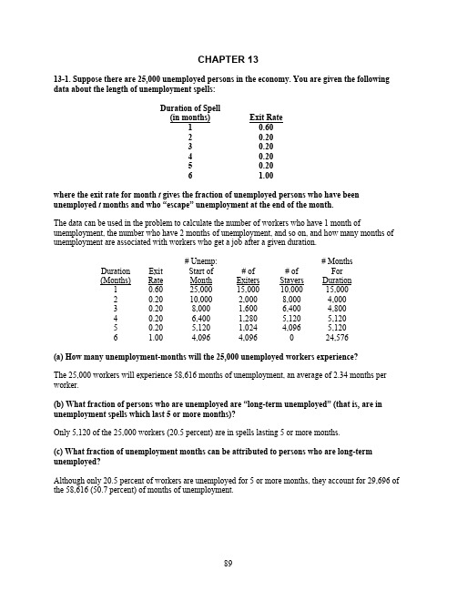
CHAPTER 1313-1. Suppose there are 25,000 unemployed persons in the economy. You are given the following data about the length of unemployment spells:Duration of Spell(in months) ExitRate1 0.602 0.203 0.204 0.205 0.206 1.00where the exit rate for month t gives the fraction of unemployed persons who have been unemployed t months and who “escape” unemployment at the end of the month.The data can be used in the problem to calculate the number of workers who have 1 month of unemployment, the number who have 2 months of unemployment, and so on, and how many months of unemployment are associated with workers who get a job after a given duration.Duration (Months) ExitRate# Unemp:Start ofMonth# ofExiters# ofStayers# MonthsForDuration1 0.60 25,000 15,00010,000 15,0002 0.20 10,000 2,000 8,000 4,0003 0.20 8,000 1,600 6,400 4,8004 0.20 6,400 1,280 5,120 5,1205 0.20 5,120 1,024 4,096 5,1206 1.00 4,096 4,096 0 24,576(a) How many unemployment-months will the 25,000 unemployed workers experience?The 25,000 workers will experience 58,616 months of unemployment, an average of 2.34 months per worker.(b) What fraction of persons who are unemployed are “long-term unemployed” (that is, are in unemployment spells which last 5 or more months)?Only 5,120 of the 25,000 workers (20.5 percent) are in spells lasting 5 or more months.(c) What fraction of unemployment months can be attributed to persons who are long-term unemployed?Although only 20.5 percent of workers are unemployed for 5 or more months, they account for 29,696 of the 58,616 (50.7 percent) of months of unemployment.(d) What is the nature of the unemployment problem in this example: too many workers losing their jobs or too many long spells?Most spells are short-lived, but workers in long spells account for most of the unemployment observed in this economy. Thus, the main problem is too many long spells.13-2. Consider Table 599 of the 2002 U.S. Statistical Abstract.(a) How many workers aged 20 or older were unemployed in the United States during 2001? How many of these were unemployed less than 5 weeks, 5 to 14 weeks, 15 to 26 weeks, and 27 or more weeks?In total, 5,554,000 workers aged 20 years or older were unemployed in the U.S. in 2001. Of these, 40 percent, or 2,221,600 workers, were unemployed for less than 5 weeks; 32.2 percent, or 1,788,388 workers, were unemployed between 5 and 14 weeks; 15.5 percent, or 860,870 workers, were unemployed15 to 26 weeks, and 12.9 percent, or 716,466 workers were unemployed for 27 or more weeks.(b) Assume that the average spell of unemployment is 2.5 weeks for anyone unemployed for less than 5 weeks. Similarly, assume the average spell is 10 weeks, 20 weeks, and 35 weeks for the remaining categories. How many weeks did the average unemployed worker remain unemployed? What percent of total months of unemployment are attributable to the workers that remained unemployed for at least 15 weeks?The total number of weeks of unemployment is calculated as:2,221,600(2.5) + 1,788,388(10) + 860,870(20) + 716,466(35) = 65,731,590months of unemployment spread over 5,554,000 unemployed workers, implies that the average unemployed worker remained unemployed for 11.835 weeks. The percent of total months of unemployment attributable to the workers that remained unemployed for at least 15 weeks is[ 860,870(20) + 716,466(35) ] / 65,731,590 = 64.34 percent.13-3. Suppose the marginal revenue from search isMR = 50 - 1.5w,where w is the wage offer at hand. The marginal cost of search isMC = 5 + w.(a) Why is the marginal revenue from search a negative function of the wage offer at hand?If the offer-at-hand is relatively low, it pays to keep on searching as the next offer is likely higher than the offer-at-hand. If the offer-at-hand is very high, however, it does not pay to keep on searching since it is unlikely that the next search will generate a higher wage offer.(b) Can you give an economic interpretation of the intercept in the marginal cost equation; in other words, what does it mean to say that the intercept equals $5? Similarly, what does it mean to say that the slope in the marginal cost equation equals one dollar?The $5 indicates the out-of-pocket search costs. Even if the offer-at-hand is zero (so that there is no opportunity cost to search), it still costs money to get to the firm and learn about the details of the potential job offer. The slope equals $1, because the costs of search also vary directly with the opportunity cost of search which is the wage offer at hand. If the wage offer at hand is $10, the opportunity cost from one more search equal $10; if the wage offer at hand is $11, the opportunity cost would be $11, and so on.(c) What is the worker’s asking wage? Will a worker accept a job offer of $15?The asking wage is obtained by equating the marginal revenue of search to the marginal cost of search, or 50 – 1.5w = 5 + w. Solving for w implies that the asking wage is $18. The worker, therefore, would not accept a job offer of $15.(d) Suppose UI benefits are reduced, causing the marginal cost of search to increase to MC = 20 + w. What is the new asking wage? Will the worker accept a job offer of $15?If we equate the new marginal cost equation to the marginal revenue equation we find that the asking wage drops to $12. The worker will now accept a wage offer of $15.13-4. (a) How does the exclusion of non-working welfare recipients affect the calculation of the unemployment rate? Use the 2002 U.S. Statistical Abstract to estimate what the 2000 unemployment rate would have been if welfare recipients had been included in the calculation.Excluding non-working welfare recipients from the unemployment rate biases the unemployment rate downward. Table 560 of the Statistical Abstract shows that the labor force in 2000 totaled 140,863,000, while the number employed totaled 135,208,000. Thus, the unemployment rate was 4.0 percent.Table 513 of the Statistical Abstract shows that 2,253,000 people received public assistance in 2000. Assuming all of these were non-working and out of the labor force, their inclusion in the calculation of the unemployment rate would increase the unemployment rate to(140,863,000 + 2,253,000 – 135,208,000) / (140,863,000 + 2,253,000) = 5.5%.(b) How does the exclusion of black market workers affect the calculation of the unemployment rate? Estimate, the best you can, what the 2000 unemployment rate would have been if workers in the underground economy had been included in the calculation.Excluding black market workers from the calculation of the unemployment rate keeps the unemployment rate artificially high. At the best, black market workers are not counted in the labor force, but at the worst, the black market workers claim to be in the labor force and without a job. The problem is that there is no (or very little) data on the black market by definition. Some researchers have estimated the underground economy to be on the order of 10 to 20 percent of activity in the U.S. Suppose half of underground economy workers have regular market jobs as well. Suppose further that of the remaining half, one half claim to be unemployed while the other half is out of the labor force. Thus, 10 percent of the unemployed workers are the number of underground economy workers in the labor force without a job: 10 percent of(140,863,000 – 135,208,000) = 565,500. An equal number say they are not in the labor force. (And twice this number is already reporting having a legitimate job.) Using these estimates, therefore, the labor force should be 140,863,000 + 565,500 = 141,428,500, while the number employed should be 135,208,000 + 565,500 + 565,500 = 136,339,000. Thus, the unemployment rate would be(141,428,500 – 136,339,000) / 141,428,500 = 3.6%.13-5. Compare two unemployed workers; the first is 25 years old and the second is 55 years old. Both workers have similar skills and face the same wage offer distribution. Suppose that both workers also incur similar search costs. Which worker will have a higher asking wage? Why? Can search theory explain why the unemployment rate of young workers differs from that of older workers?The marginal revenue of search depends on the length of the payoff period. Younger workers have the most to gain from obtaining higher paying jobs, since they can then collect the returns from their search investment over a longer expected work-life. As a result, it pays for younger workers to set their asking wage at a relatively high level. This implies that younger workers will tend to have higher unemployment rates and longer spells of unemployment than older workers.13-6. Suppose the government proposes to increase the level of UI benefits for unemployed workers.A particular industry is now paying efficiency wages to its workers in order to discourage them from shirking. What is the effect of the proposed legislation on the wage and on the unemployment rate for workers in that industry?The introduction of UI benefits shifts the no-shirking supply curve upwards (from NS to NS′), because a higher wage would have to be paid in order to attract the same number of workers who do not shirk. As a result, the new equilibrium (point Q′) entails a higher efficiency wage and leads to a larger number of unemployed workers.Dploym ent13-7. It is well known that more-educated workers are less likely to be unemployed and haveshorter unemployment spells than less-educated workers. Which theory(ies), the job search model, the sectoral shifts hypothesis, or the efficiency wage model, can explain this empirical correlation?Two of the theories in question can be formulated in such a way that they each predict that more-educated workers will have less unemployment and shorter spells of unemployment than less-educated workers.The job search model suggests that highly educated workers would have a lower unemployment rate either if they have relatively higher search costs or relatively lower gains from search. It could then be argued, for example, that search costs are (relatively) higher for highly-educated workers than for less-educated workers, perhaps because the nature of the job match between a highly educated worker and a firm is much more complex than the type of job match required between the firm and a worker who does repetitive tasks.Similarly, it is plausible to argue that it is easier to retool a highly-educated worker than a less-educated worker. The decline in demand in particular industries, then, leads to sectoral shift that can be better weathered by highly-educated workers.The efficiency wage model, however, has a harder time explaining the correlation. Presumably, the output of highly-educated workers is more difficult to measure than the output of less-educated workers. As a result, efficiency wages are more likely to arise in industries that employ highly-educated workers, and these industries (which pay above-market wages) would have to maintain a pool of unemployed workers in order to keep the employed workers in line.13-8. Suppose a country has 100 million inhabitants. The population can be divided into the employed, the unemployed, and the persons who are out of the labor force (OLF). In any given year, the transition probabilities among the various categories are given by:Moving Into:Employed Unemployed OLFEmployed 0.94 0.02 0.04 Unemployed 0.20 0.65 0.15 Moving From: OLF 0.05 0.03 0.92These transition probabilities are interpreted as follows. In any given year, 2 percent of the workers who are employed become unemployed; 20 percent of the workers who are unemployed find jobs, and so on. What will be the steady-state unemployment rate?Use E for the number of employed people, U for the number of unemployed, and N for the number not participating. The flows of people among the three categories can be found by multiplying these numbers with respective probabilities in the table. In the steady-state, the flows into each category must exactly balance the outflows. This produces the following equations:Employed: E = .94E + .20U + .05NUnemployed: U = .02E + .65U + .03NOLF: N = .04E + .15U + .92NOnly two of the three equations can be used, however, as E + U + N = 100 million. The steady-state solutions for E, U, and N can now be found with brute force algebra. The solution is that 54.273 million are employed, 6.466 million are unemployed, and 39.261 million are not in the labor force. The steady-state unemployment rate is then%646.10739.60466.6100100=×=×+=E U U u .13-9. Consider an economy with 250,000 adults, of which, 40,000 are retired senior citizens, 20,000 are college students, 120,000 are employed, 8,000 are looking for work, and 62,000 stay at home. What is the labor force participation rate? What is the unemployment rate?The labor force participation rate = ( 120,000 + 8,000 ) / 250,000 = 51.2 percent.The unemployment rate = 8,000 / ( 120,000 + 8,000 ) = 6.25 percent.13-10. Consider an economy with 3 types of jobs. The table below shows the jobs, the frequency with which vacancies open up on a yearly basis, and the income associated with each job. Searching for a job costs $C per year and generates at most 1 job offer. There is a 20 percent chance of not generating any offer in a year. (Note: the expected search duration for a job with probability p of appearing is 1/p years.)Job Type Frequency IncomeA 30 percent $60,000B 20 percent $100,000C 30 percent $80,000As a function of C , specify the optimal job search strategy if the worker maximizes her expected income net of search costs.There are four possible strategies for the worker: accept any job paying at least $100,000, accept any job paying at least $80,000, accept any job paying at least $60,000, or do not search for a job.Under the first strategy, the worker will only accept a B job. The expected search time for a B job is 5 years. Thus, the expected value of this strategy is $100,000 – 5C .Under the second strategy, the worker will accept a B or a C job. The expected search time, therefore, is 2 years (i.e., there is a 50 percent chance of receiving a B or a C job in a year, so the search time is 1/0.5 =2). Thus, the expected value of this strategy isC C 2000,88$2)000,80($3.02.03.0)000,100($3.02.02.0−=−+++.Under the third strategy, the worker will accept any of the three jobs. The expected search time, therefore, is 1.25 years, and the expected value of this strategy isC C 25.1500,77$25.1)000,60($8.03.0)000,80($8.03.0)000,100($8.02.0−=−++.Under the fourth strategy, the worker does not search, and therefore does not find a job or incur search costs, for an expected payoff of $0.One can now compare the four expected payoffs to determine that the optimal search strategy is:Accept the first B job if C < $4,000.Accept the first B or C job if $4,000 # C < $14,000.Accept the first job of any kind if $14,000 # C < $62,000.Don’t search if $62,000 # C .13-11. (a) A country is debating whether to fund a national database of job openings and giving all unemployed workers free access to it. What effect would this plan have on the long-rununemployment rate? What effect would this plan have on the average duration of unemployment? Why?Lower search costs would probably increase the unemployment rate. Lower search costs (similar to extended UI benefits) will cause workers to keep their asking wage higher for a longer time. Thus, unemployed workers will be more selective in the jobs they accept. The result is that workers remain unemployed for longer periods of time. It is also possible that lower search costs will entice workers to quit their jobs in order to look for a better job. This will also increase the unemployment rate.(b) A country is debating whether to impose a $10,000 tax on employers for every worker they lay-off. What effect would this plan have on the long-run unemployment rate? What effect would this plan have on the average duration of unemployment?This policy would cause firms, in the long-run, to be very cautious in hiring new workers. (This cautious behavior is evident in Japan and some countries in Europe. The UI system in the US may also cause firms to be a bit cautious in hiring new workers.) Thus, the unemployed will remain unemployed for longer durations. The effect on the unemployment rate is a little ambiguous. The unemployment rate wouldlikely increase in the long-run, but one could also argue that the end result will be less labor turnover and, therefore, a lower rate of unemployment, especially if unemployed workers under the proposed rules are more easily discouraged and exit the labor force all together.。

劳动经济学鲍哈斯第七版第三章答案

劳动经济学鲍哈斯第七版第三章答案1、已达到预定可使用状态但未办理竣工决算的固定资产，应根据（）作暂估价值转入固定资产，待竣工决算后再作调整。

[单选题] *A.市场价格B.计划成本C.估计价值(正确答案)D.实际成本2、A企业2014年12月购入一项固定资产，原价为600万元，采用年限平均法计提折旧，使用寿命为10年，预计净残值为零，2018年1月该企业对该项固定资产的某一主要部件进行更换，发生支出合计400万元，符合固定资产确认条件，被更换的部件的原价为300万元。

则对该项固定资产进行更换后的原价为( )万元。

[单选题] *A.210B.1 000C.820D.610(正确答案)3、由投资者投资转入的无形资产，应按合同或协议约定的价值，借记“无形资产”科目，按其在注册资本所占的份额，贷记“实收资本”科目，按其差额记入（）科目。

[单选题] *A.“资本公积—资本溢价”(正确答案)B.“营业外收入”C.“资本公积—其它资本公积”D.“营业外支出”4、企业收取包装物押金及其他各种暂收款项时，应贷记（）科目。

[单选题] *A.营业外收入B.其他业务收入C.其他应付款(正确答案)D.其他应收款5、2018年3月，A 公司提出一项新专利技术的设想，经研究，认为研制成功的可能性很大，于2018年4月开始研制。

2019年3月研制成功，取得了专利权。

研究阶段共发生支出500万元，开发阶段发生相关支出1 000万元，其中包含满足无形资产确认条件的支出为800万元。

企业该项专利权的入账价值为( ) 万元。

[单选题] *A.1 500B.800(正确答案)C.1 000D.5006、根据准则的规定，企业收到与日常活动无关的政府补助应当计入（）科目。

[单选题] *A.投资收益B.其他业务收入C.主营业务收入D.营业外收入(正确答案)7、．（年浙江省高职考）下列项目中，不属于企业会计核算对象的经济活动是（）[单选题] *A购买设备B请购原材料(正确答案)C接受捐赠D利润分配8、企业开出的商业汇票为银行承兑汇票，其无力支付票款时，应将应付票据的票面金额转作（）。

现代劳动经济学课后【伊兰伯格】课后习题答案

INSTRUCTOR'S MANUALto accompanyEhrenberg & SmithModern Labor Economics:Theory & Public PolicyEighth EditionRobert S. SmithCornell UniversityRobert M. WhaplesWake Forest UniversityLawrence WohlGustavus Adolphus UniversityCopyright 2003 Addison-Wesley, Inc.All rights reserved. Printed in the United States of America. No part of this book may be used or reproduced in any manner whatsoever without written permission from the publisher, except testing materials and transparency masters may be copied for classroom use. For information, address Addison-Wesley Higher Education, Pearson PLC 75 Arlington Street, Suite 300, Boston, Massachusetts 02116.A NOTE TO THE INSTRUCTORThis Instructor's Manual is intended to summarize the content of the eighth edition of Modern Labor Economics: Theory and Public Policy in a way that explains our pedagogical strategy. Summarized briefly, we believe that labor economics can be best learned if students are (1) able to see the "big picture" early on, so that new concepts can be placed in perspective; (2) moved carefully from concepts they already know to new ones; (3) motivated by seeing the policy implications or inherently interesting insights generated by the concepts being taught. To this last end, we discuss policy issues in every chapter and, in addition, employ "boxed examples" to demonstrate in historical, cross-cultural, or applied managerial settings the power of the concepts introduced.The text is designed to be accessible to students with limited backgrounds in economics. We do employ graphic analyses and equations as learning aids in various chapters; however, we are careful to precede their use with verbal explanations of the analyses and to introduce these aids in a step-by-step fashion. To help students in the application of concepts to various issues, we have printed answers to the odd-numbered review questions for each chapter at the back of the book.We have also endeavored to put together a text that, while accessible to all, is a comprehensive and up-to-date survey of modern labor economics. There are 9 chapter appendices designed to be used with more advanced students in generating additional insights.In the first part of this Instructor's Manual, we present a brief overview and the general plan of Modern Labor Economics. We then present a chapter-by-chapter review of the concepts presented in the text. In the discussion of each chapter we list the major concepts or understandings covered, and in some cases suggest topics or sections that could be eliminated if time must be conserved. We also present our answers to the even-numbered review questions at the end of each chapter.An important part of this Instructor's Manual are the suggested essay questions related to each chapter. We present a few suggested essay questions for each chapter.Table of ContentsClick on the chapter title to jump directly to that page.Overview of the Text 1 Chapter 1 Introduction 4 Chapter 2 Overview of the Labor Market8 Chapter 3 The Demand for Labor14 Chapter 4 Labor Demand Elasticities20 Chapter 5 Quasi-Fixed Labor Costs and Their Effects on Demand26 Chapter 6 Supply of Labor to the Economy: The Decision to Work32 Chapter 7 Labor Supply: Household Production, the Family, and the Life Cycle37 Chapter 8 Compensating Wage Differentials and Labor Markets45 Chapter 9 Investments in Human Capital: Education and Training51 Chapter 10 Worker Mobility: Migration, Immigration, and Turnover57 Chapter 11 Pay and Productivity62 Chapter 12 Gender, Race, and Ethnicity in the Labor Market68 Chapter 13 Unions and the Labor Market77 Chapter 14 Inequality in Earnings84 Chapter 15 Unemployment88OVERVIEW OF THE TEXTINTRODUCTION/REVIEW: Chapters 1 and 2Chapter 1 - IntroductionAppendix 1A - Statistical Testing of Labor Market Hypotheses Chapter 2 - Overview of the Labor MarketChapters 1 and 2 introduce basic concepts of labor economics. They are written to be accessible to students without backgrounds in intermediate theory, and can, therefore, be used as building blocks when a professor must "begin at the beginning." If the course is being taught to economics majors with intermediate microeconomics as a prerequisite, these chapters may be skipped or skimmed quickly as a review.An appendix to Chapter 1 introduces the student to econometrics. The purpose of this appendix is to present enough of the basic econometric concepts and issues to permit students to read papers employing ordinary least squares regression techniques. We strongly recommend assigning Appendix 1A in courses requiring students to read empirical papers in the field. We also recommend (in footnote 3 of the appendix) an introductory econometrics text that could be assigned by instructors who wish to go beyond our introductory treatment.THE DEMAND FOR LABOR: Chapters 3-5Chapter 3 - The Demand for LaborAppendix 3A - Graphic Derivation of a Firm's Labor Demand Curve Chapter 4 - Labor Demand ElasticitiesAppendix 4A - International Trade and the Demand for Labor: Can High-Wage Countries Compete?Chapter 5 - Quasi-Fixed Labor Costs and Their Effects on DemandThe demand for labor is discussed first primarily because we believe that the supply of labor is a more complex topic in many ways. Before analyzing the labor/leisure choice and household production, we first introduce students to the employer side of the market. For instructors who desire to cover topics concerned with the decision to work first, however, we note that Chapters 6 and 7, which deals with that decision, are self-contained. Therefore, nothing would be lost if Chapters 6 and 7 were taught ahead of Chapters 3, 4, and 5.In Chapter 3 the principal question analyzed is why demand curves slope downward. In Chapter 4 we move to a discussion of the elasticity of demand, and analyze the determinants of the precise relationship between wages and employment. The concepts are used to analyze how technological change and foreign trade affect labor demand. Finally, Chapter 5 analyzes the quasi-fixed nature of many labor costs and the ways these costs affect the demand for labor.SUPPLY OF LABOR TO THE ECONOMY: Chapters 6 and 7Chapter 6 - Supply of Labor to the Economy: The Decision to WorkChapter 7 - Labor Supply: Household Production, the Family, and the Life Cycle Chapters 6 and 7 analyze the decision of an individual to work for pay. The traditional analysis of the labor/leisure choice is given in Chapter 6, while in Chapter 7 the decision to work for pay is placed in the context of household production. The essential features of the decision to work for pay are included in Chapter 6. In one-quarter courses or courses in which time is scarce, Chapter 7 could be skipped; however, doing so would eliminate analyses of family labor supply decisions as well as labor supply decisions in the context of the life cycle.As noted above, Chapters 6 and 7 are designed to be self-contained for the convenience of instructors who wish to teach labor supply ahead of labor demand.FACTORS AFFECTING THE CHOICE OF EMPLOYMENT: Chapters 8-10 Chapter 8 - Compensating Wage Differentials and Labor MarketsAppendix 8A - Compensating Wage Differentials and Layoffs Chapter 9 - Investments in Human Capital: Education and TrainingAppendix 9A - A "Cobweb” Model of Labor Market AdjustmentAppendix 9B - A Hedonic Model of Earnings and Educational Level Chapter 10 - Worker Mobility: Migration, Immigration, and TurnoverOnce they have decided to seek employment, prospective workers encounter important choices concerning their occupation and industry, as well as the general location of their employment. Chapters 8 through 10 analyze these choices, with Chapters 8 and 9 focusing on industry/occupational choice and Chapter 10 on the choice of a specific employer and the location of employment. More particularly, Chapter 8 presents an analysis of job choice within the context of jobs that differ along nonpecuniary dimensions. Chapters 9 and 10 analyze issues affecting worker investments in skill acquisition (Chapter 9) and job change (Chapter 10), and both employ the concepts of human capital theory. All three chapters contain appendices of interest to instructors who wish to teach more advanced material.ANALYSES OF SPECIAL TOPICS IN LABOR ECONOMICS: Chapters 11-15 Chapter 11 - Pay and ProductivityChapter 12 - Gender, Race, and Ethnicity in the Labor MarketAppendix 12A - Estimating "Comparable Worth" Earnings Gaps: AnApplication of Regression AnalysisChapter 13 - Unions and the Labor MarketAppendix 13A - Arbitration and the Bargaining Contract ZoneChapter 14 - Inequality in EarningsAppendix 14A - Lorenz Curves and Gini CoefficientsChapter 15 - UnemploymentHaving presented basic concepts and analytical tools necessary to understand the demand and supply sides of the labor market, we now move to analyses of special topics: compensation, discrimination, unions, inequality, and unemployment. A complete analysis of all these topics requires an understanding of behavior on both the demand and supply sides of the market, and these chapters are built upon the preceding ten. No new analytical tools are introduced in these chapters.The chapters on unionism (Chapter 13) and discrimination (Chapter 12) deal with issues typically covered in labor economics courses, but they are more comprehensive than most other texts. It should be noted that the appendix to Chapter 12 includes an application of regression analysis. The chapter on inequality is unique and can be skipped without a loss in coverage of conventional material; however, it is written in a way that provides a review of material in previous chapters.CHAPTER 1 - INTRODUCTIONBecause the textbook stresses economic analysis as it applies to the labor market, students must understand the ways economic analyses are used. The basic purpose of Chapter 1 is to introduce students to the two major modes of economic analysis: positive and normative. Because both modes of analysis rest on some very fundamental assumptions, Chapter 1 discusses the bases of each mode in some detail.In our treatment of positive economics, the concept of rationality is defined and discussed, as is the underlying concept of scarcity. There is, in addition, a lengthy discussion of what an economic model is, and an example of the behavioral predictions flowing from such a model is presented. The discussion of normative economics emphasizes its philosophical underpinnings and includes a discussion of the conditions under which a market would fail to produce results consistent with the normative criteria. Labor market examples of governmental remedies are provided.The appendix to Chapter 1 introduces the student to ordinary least squares regression analysis. It begins with univariate analysis, introduced in a graphical context, explaining the concepts of dependent and independent variables, the "intercept" and "slope" parameters, the "error term," and the t statistic. The analysis then moves to multivariate analysis and the problem of omitted variables.List of Major Concepts1. The essential features of a market include the facilitation of contact between buyersand sellers, the exchange of information, and the execution of contracts.2. The uniqueness of labor services affects the characteristics of the labor market.3. Positive economics is the study of economic behavior, and underlying this theory ofbehavior are the basic assumptions of scarcity and rationality.4. Normative economics is the study of what "should be," and theories of socialoptimality are based in part on the underlying philosophical principle of "mutualbenefit. "5. A market "fails" when it does not permit all mutually beneficial trades to take place,and there are three common reasons for such failure.6. A governmental policy is "Pareto-improving" if it encourages additional mutuallybeneficial transactions. At times, though, the goal of improving Pareto efficiency conflicts with one of generating more equity.7. The concept that governmental intervention in a market may be justified on groundsother than the principle of mutual benefit is discussed (for example, governmentintervention may be justified on the grounds that income redistribution is a desirable social objective).8. (Appendix) The relationship between two economic variables (e.g., wages and quitrates) can be plotted graphically; this visual relationship can also be summarized algebraically.9. (Appendix) A way to summarize a linear relationship between two variables isthrough ordinary least squares regression analysis -- a procedure that plots the "best"line (the one that minimizes the sum of squared deviations) through the various data points. The parameters describing this line are estimated, and the uncertaintysurrounding these estimates are summarized by the standard error of the estimate. 10. (Appendix) Multivariate procedures for summarizing the relationship between adependent and two or more independent variables is a generalization of the univariate procedure, and each coefficient can be interpreted as the effect on the dependentvariable of a one-unit change in the relevant independent variable, holding the other variables constant.11.(Appendix) If an independent variable that should be in an estimating equation is leftout, estimates of the other coefficients may be biased away from their true values. Answers to Even-Numbered Review Questions2. Are the following statements "positive" or "normative"? Why?a. Employers should not be required to offer pensions to their employees.b. Employers offering pension benefits will pay lower wages than they would if they didnot offer a pension program.c. If further immigration of unskilled foreigners is prevented, the wages of unskilledimmigrants already here will rise.d. The military draft compels people to engage in a transaction they would notvoluntarily enter into; it should therefore be avoided as a way of recruiting military personnel.e. If the military draft were reinstituted, military salaries would probably fall. Answer: (a) normative (b) positive (c) positive (d) normative (e) positive4. What are the functions and limitations of an economic model?Answer: The major function of an economic model is to strip away real world complexities and focus on a particular cause/effect relationship. In this sense an economic model is analogous to an architect's model of a building. An architect may be interested in designing a building that fits in harmoniously with its surroundings, and in designing such a building the architect may employ a model that captures the essentials of his or her concerns (namely, appearance) without getting into the complexities ofplumbing, electrical circuits, and the design of interior office space. Similarly, an economic model will often focus on a particular kind of behavior and ignore complexities that are either not germane to that behavior or only of indirect importance.Models used to generate insights about responses to a given economic stimulus are often not intended to forecast actual outcomes. For example, if we are interested in bow behavior is affected by stimulus B, with factors C, D, and E held constant, our model may not correctly forecast the observed behavior if stimuli C through E also change.6. A few years ago it was common for state laws to prohibit women from working morethan 40 hours a week. Using the principles underlying normative economics, evaluate these laws.Answer: Laws preventing women from working more than 40 hours per week essentially blocked mutually beneficial transactions. There were women who wanted to work more than 40 hours a week, and there were employers who wanted to employ them for more than 40 hours a week. The restrictions upon their employment prevented these transactions from occurring and therefore made both the women and their potential employers worse off.8. “Government policies as frequently prevent Pareto efficiency as they enhance it.”Comment.Answer. Achieving Pareto efficiency requires the completion of all mutually beneficial transactions. Ideally, government would step in to provide information is that is blocking mutually beneficial transactions or to establish markets (or market substitutes) when markets do not exist. However, governments also have power to prevent transactions or distort prices, both of which can prevent the completion of mutually beneficial transactions. Government regulations can outlaw certain transactions that the parties to them would consider mutually beneficial (the text mentions laws that historically prevented women from working more than 40 hours per week). Government also has the power to distort prices by setting minimum wages, mandating premiums for overtime work, and so forth.Answers to Even-Numbered Problems2. (Appendix) Suppose that a least squares regression yields the following estimate:Wi = -1 + .3Ai, where W is the hourly wage rate (in dollars) and A is the age in years.A second regression from another group of workers yields this estimate:Wi = 3 + .3Ai - .01(Ai)2.a. How much is a 20-year-old predicted to earn based on the first estimate?b. How much is a 20-year-old predicted to earn based on the second estimate? Answer: a. W = -1 + .3x20 = 5 dollars per hour.b. W = 3 + .3x20 - .01x20x20 = 3 + 6 - 4 = 5 dollars per hour.Suggested Essay Questions1. Child labor is an issue that has been discussed a lot recently. From the perspective ofnormative economics, explain the problem with child labor.Answer: Pareto efficiency requires that transactions have mutual benefits, and this can be assured only if the transactions are voluntary and take place with complete information. Children may be compelled by their parents to work, and they have limited capacities to make informed decisions even in the absence of compulsion.2. A law in one town of a Canadian province limits large supermarkets to just fouremployees on Sundays. Analyze this law using the concepts of normative economics. Answer. There are no doubt large supermarkets that want to hire workers on Sundays (because there are consumers who want to shop on Sundays), and there are no doubt employees who could be induced – perhaps by higher wages – to work on Sundays. A law preventing such work prevents a mutually beneficial transaction.CHAPTER 2 - OVERVIEW OF THE LABOR MARKETOur goal in this text is to move students along very carefully from what they do know to the mastery of new concepts. It is our belief that students learn most efficiently if they can associate these new ideas with an overall framework, and it is the purpose of Chapter 2 to provide that framework. This chapter has both a descriptive and an analytical purpose. One aim is to introduce students to the essential concepts, definitions, magnitudes, and trends of widely used labor market descriptors. To this purpose, the chapter discusses and presents data on such topics as the labor force, unemployment, the distribution of employment, and the level of (and trends in) labor earnings. The second aim is to provide students with an overview of labor market analysis. To this end, we discuss basic concepts of demand and supply so that students will be able to see their interaction at the very outset.We start the overview with a discussion of demand schedules and their corresponding demand curves. Particular attention is given to the distinction between movement along a curve and shifts of a curve. Distinctions between individual and more aggregated demand curves are discussed, as is the distinction between short-run and long-run demand curves.A similar discussion and set of distinctions are made for the supply side of the market. After both the demand and supply sides of the market have been discussed and generally modeled, we turn to the question of wage determination and wage equilibrium. Forces that can alter market equilibria are comprehensively discussed, and the chapter's major concepts are reinforced by discussions of the effects of unions, the existence of disequilibrium, and the concept of being "overpaid" or "underpaid" (including a discussion of economic rents). The chapter ends with a discussion of unemployment across various countries.List of Major Concepts1. The labor market and its various subclassifications (national, regional, local; external,internal; primary, secondary) are defined.2. The "labor force" consists of those who are employed or who are seeking work, andmajor trends in labor force participation rates are discussed.3. The "unemployed" are those who are not employed but are seeking work (or awaitingrecall); trends in the unemployment rate are noted.4. Changes in the industrial and occupational distribution of employment are facilitatedby the labor market, which also facilitates adjustments to the "birth" and "death" of job opportunities.5. The distinction between nominal and real wage rates is made, and the calculation ofreal wages is illustrated.6. Distinctions among wage rates, earnings, total compensation, and income aredepicted graphically.7. The labor market is one of three major markets with which an employer must deal; inturn, labor market outcomes (terms of employment and employment levels) areaffected by both product and capital markets.8. The concepts underlying a labor demand schedule are associated with productdemand, the choice of technology, and the supply schedule of competing factors of production; scale and substitution effects are ultimately related to these forces.9. Underlying a supply schedule for labor are the alternatives workers have and theirpreferences regarding the job's characteristics.10. Distinctions between individual and market demand and supply curves are discussed.11. Movements along, rather than shifts of, demand and supply curves occur when wagesof the job in question change; when a variable not shown on the graph changes, the curves tend to shift.12. The interaction of market demand and supply determines the equilibrium wage.13. Changes in the equilibrium wage rate are caused by shifts in either the demand orsupply curves. Disequilibium will persist if the wage is not allowed to adjust to shifts in demand or supply.14. The concepts of "overpaid" and "underpaid" compare the actual wage to theequilibrium (market) wage rate.15. Individuals paid more than their reservation wage are said to obtain an "economicrent."16. The concepts of shortage and surplus are directly related to the relationship betweenactual and equilibrium wage rates.17. Unemployment rates, and especially long-term unemployment rates, have risen inEurope relative to the United States and Canada over the recent decade; this rise may reflect the existence of relatively stronger nonmarket forces in Europe.Answers to Even-Numbered Review Questions2. Analyze the impact of the following changes on wages and employment in agiven occupation:a.)A fall in the danger of the occupation.b.)An increase in product demand.c.)Increased wages in alternative occupations.Answer: (a) A fall in the danger of the occupation, other things being equal, should increase the attractiveness of that occupation, shifting the supply curve to the right and causing employment to rise and wages to fall.(b) An increase in product demand will shift the demand for labor curve to the right causing both wages and employment to increase.(c) Increased wages in other occupations will render them relatively more attractive than they were before and cause the supply curve to the occupation in question to shift to the left. This will cause employment in this market to fall and wages to rise.4. Suppose a particular labor market were in market-clearing equilibrium. What couldhappen to cause the equilibrium wage to fall? If all money wages rose each year, how would this market adjust?Answer: Starting from the position of equilibrium, a labor market could experience a fall in the equilibrium wage if either the demand curve shifts to the left or the supply curve shifts to the right. While market wages are usually stated in nominal terms, their relationship to the prices of both consumer and producer products is of ultimate importance. Therefore, both parties to the employment relationship are, in the last analysis, concerned with the real wage rate. The real wage rate can fall when the nominal wage rate is rising if prices of consumer and producer products rise even more quickly.6. How will a fall in the civilian unemployment rate affect the supply of recruits for thevolunteer army? What will be the effect on military wages?Answer: Supply curves to a given occupation are drawn holding alternative opportunities constant. If those opportunities become more attractive, the supply curve to the given occupation will shift left and tend to drive up wages. Thus, a fall in the unemployment rate will shift the army's supply curve to the left (there will be fewer recruits at each army wage rate), and the army's wages will be driven up.8. Suppose that the Consumer Product Safety Commission issues a regulation requiringan expensive safety device to be attached to all power lawnmowers. This device does not increase the efficiency with which the lawnmower operates. What, if anything, does this regulation do to the demand for labor of firms manufacturing powerlawnmowers? Explain.Answer: This regulation would cause the demand for labor curve of the firms that manufacture power mowers to shift to the left. The demand for labor is in part derived from product demand. Because it is more costly now to manufacture lawnmowers, the prices that will be charged to consumers will rise. This price increase will move the firm upward and to the left along its product demand curve. With less product demanded for any given wage rate paid to workers, the end result is a leftward shift of the labor demandcurve. (If, however, consumer preferences for greater safety were to shift the product demand curve to the right, employment losses would be mitigated.)10. Suppose we observe that employment levels in a certain region suddenly decline as aresult of (i) a fall in the region's demand for labor, and (ii) wages that are fixed in the short run. If the new demand for labor curve remains unchanged for a long period and the region's labor supply curve does not shift, is it likely that employment in theregion will recover? Explain.Answer: The initial response to a leftward shift in the labor demand curve in the context of fixed wages is for there to be a relatively large decline in employment. This decline in employment is larger than the ultimate decline in employment. The initial disequilibrium between demand and supply in the labor market should force wages down in the long run, and as wages decline firms will move downward along their labor demand curves andwill begin to employ more labor. However, employment in the region would recover to its prior level (assuming no subsequent shifts in demand or supply curves) only if the supply curve was vertical; if supply curves are upward-sloping, the declining wage will cause some withdrawal of labor from the market and employment will not recover to its prior level.Answers to Even-Numbered Problems2.Suppose that the supply curve for school teachers is Ls = 20,000 + 350W and thedemand curve for school teachers is Ld = 100,000 – 150W, where L = the number of teachers and W = the daily wage.a. Plot the demand and supply curves.b. What are the equilibrium wage and employment level in this market?c. Now suppose that at any given wage 20,000 more workers are willing to work asschool teachers. Plot the new supply curve and find the new wage and employment level. Why doesn't employment grow by 20,000?Answer: a. See the figure. Plot the Ld and Ls curves by solving for desired employment at given wage rates. If W = 500, for example, employers desire 25,000 workers (Ld = 100,000 – 150x500); if W = 400, they would desire 40,000. Since the equation above is for a straight line, drawing a line using these two points gives us the demand curve. Use the same procedure for the labor supply curve.。

劳动经济学课后习题参考答案 (1)

《劳动经济学》课后思考题参考答案第一章绪论二、思考题1．如何理解劳动经济学的价值？（1）劳动经济学研究的是社会经济问题。

例如，民工荒、政府要求增加最低工资、劳动生产率下降、农民工工资急剧上升、工资增长不均等、工作培训、国有企业高管人员的高工资受到质疑、收入分配不平、农村移民增加、劳动力市场全球化扩大等等。

（2）数量上的重要性。

在西方经济中，大部分国民收入并不是来源于资本收入（利润、租金和利息），而是来源于工资。

绝大多数居民户的主要收入来源是提供劳务。

从数量上看，劳动才是我们最重要的经济资源。

（3）独有的特性。

劳动力市场的交易完全不同于产品市场的交易。

劳动力市场是一个极有意义和复杂的场所。

劳动力市场的复杂性意味着供给和需求概念在应用于劳动力市场时必须做出重大的修改和调整。

在供给方面，劳动者“出售”给雇主的劳务与该劳动者不可分离。

除了货币报酬，工人还关注工作的健康和安全性、工作难度、就业稳定性、培训和晋升机会等，这类非货币因素也许与直接收入同样重要。

这样，工人的供给决策要比产品市场的供给概念复杂得多。

（4）收益的广泛性。

无论是个人还是社会，都可以从劳动经济学中得到许多启示和教益。

从劳动经济学得到的信息和分析工具有助于人们做出与劳动力市场有关的决策。

从个人角度看。

大量内容将直接与我们有关，如工作搜寻、失业、歧视、工资、劳动力流动等。

对于企业管理者来说，从对劳动经济学的理解中所得到的知识背景和分析方法，对做出有关雇用、解雇、培训和工人报酬等方面的管理决策也应该是十分有用的。

从社会角度看，了解劳动经济学将使人们成为更有知识、更理智的公民。

2．劳动经济学的研究方法有哪些？首先要明确劳动经济学的基本假设。

劳动经济学的假设主要表现在以下四个方面：（1）资源的相对稀缺性。

如同商品和资本是稀缺的一样，劳动力资源也是有限的。

时间、个人收入和社会资源的稀缺性构成了经济学分析的基本前提。

（2）效用最大化。

由于劳动资源的稀缺性，人类社会进行生产经营活动时，必须研究劳动资源的合理配置和利用。

《劳动经济学》作者Borjas习题答案

《劳动经济学》作者Borjas习题答案CHAPTER 66-1. Politicians who support the green movement often argue that it is profitable for firms to pursue a strategy that is “environmentally correct” (for example, by building factories that do not pollute and are not noisy), because workers will be willing to work in environmentally correct factories at a lower wage rate. Evaluate the validity of this claim.If it is profitable for firms to build factories that do not pollute and are not noisy, they would have been built already. After all, firms could build these profit-maximizing factories and attract persons to work at these factories at lower wages because no compensating differential would be needed. The fact that compensating differentials exist and that governments attempt to regulate the quality of the workplace implies that providing these amenities to workers is more costly than cost-saving.6-2. Suppose wages and health insurance are the only two job characteristics workers care about. Describe the relationship between the wage level in a particular job and whether the job offers health insurance if the government does not require employers to offer health insurance to their workers. What happens to the wage structure if the government requires all firms to provide a standard package of health insurance to their workers?When the government does not require employers to offer health insurance, workers would prefer to work in those firms that offer health insurance and would be willing to pay for the right to work in such firms (assuming that all workers prefer to have health insurance). In other words, jobs that offered health insurance would pay less than jobs that did not offer such plans. When the government mandates that all employers offer health insurance to workers, the wage in those firms that had provided either no health insurance or a “substandard” package would fall and the wage would eventually be the same in all jobs. 6-3. Workers choose to work a risky or a safe job. Suppose there are 100 workers in the economy. Worker 1’s reservation price (for accepting the risky job) is $1; worker 2’s reservation price is $2, and so on. Because of technological reasons, there are only 10 risky jobs. What is the equilibrium wage differential between safe and risky jobs? Which workers will be employed at the risky firm? Suppose now that an advertising campaign paid for by the employers who offer risky jobs stresses the excitement associated with “the thrill of injury,” and this campaign changes the attitudes of the work force toward being employed in a risky job. Worker 1 now has a reservation price of -$10 (that is, she is willing to pay $10 for the right to work in the risky job); worker 2’s reservation price is -$9, and so on. There are still only 10 risky jobs. What is the new equilibrium wage differential? The supply curve to the risky job is given by the fact that worker 1 has a reservation price of $1, worker 2 has a reservation price of $2, and so on. As the figure below illustrates, this supply curve (given by S) is upward sloping, and has a slope of 1. The demand curve (D) for risky jobs is perfectly inelastic at 10 jobs. Market equilibrium is attained where supply equals demand so that 10 workers are employed in risky jobs; the market compensating wage differential is $10 since this is what it takes to entice the marginal (tenth) worker to accept a job offer from a risky firm. Note that the firm employs those workers who least mind being exposed to risk.If tastes towards risk change, the supply curve shifts down to S′ and the market equilibrium is attained when the compensating wage differential is -$1. This is the compensating differential required to hire the marginal worker (that is, the 10th worker). Note that this compensating differential implies that eventhough most workers (from worker 12 onwards) dislike risk, the market determines that risky jobs will pay less than safe jobs.6-4. Suppose all workers have the same preferences represented byU w x ,=?2where w is the wage and x is the proportion of the firm’s air that is composed of toxic pollutants. There are only two types of jobs in the economy, a clean job (x = 0) and a dirty job (x = 1). Let w 0 be the wage paid by the clean job and w 1 be the wage paid by the polluted job. If the clean job pays $16 per hour, what is the wage in dirty jobs? What is the compensating wage differential?If all persons have the same preferences regarding working in a job with polluted air, market equilibrium requires that the utility offered by the clean job be the same as the utility offered by the dirty job, otherwise all workers would move to the job that offers the higher utility. This implies that:)1(2)0(210?=?w w => .2161?=wSolving for w 1 implies that w 1 = $36. The compensating wage differential, therefore, is $20.C om pensatin gDm ent6-5. Suppose a drop in the compensating wage differential between risky jobs and safe jobs has been observed. Two explanations have been put forward:Engineering advances have made it less costly to create a safe working environment.The phenomenal success of a new action serial “Die On The Job!” has imbued millions ofviewers with a romantic perception of work-related risks.Using supply and demand diagrams show how each of the two developments can explain the drop in the compensating wage differential. Can information on the number of workers employed in the risky occupation help determine which explanation is the right one?The engineering advances make it cheaper for firms to offer safe jobs, and hence reduce the gain from switching from a safe environment to a risky one. This will shift the demand curve for risky jobs in and reduce the compensating wage differential (Figure 1). Note that the equilibrium number of workers in risky jobs goes down.The glamorization of job-related risks may make people more willing to take these risks. This shiftssupply to the right and reduces the compensating differential (Figure 2). Note that the equilibrium number of workers in risky jobs goes up.Thus, information on whether employment in the risky sector increased or decreased can help discern between the two competing explanations.Figure 1. Labor Market for Risky JobsCompensatingDifferentialE new E old Number of Workers in Risky Jobs(w 1 – w 0 )old (w 1 – w 0 )Figure 2. Labor Market for Risky Jobs6-6. Consider a competitive economy that has four different jobs that vary by their wage and risk level. The table below describes each of the four jobs.Job Risk ( r ) Wage ( w )A 1/5 $3B 1/4 $12C 1/3 $23D 1/2 $25All workers are equally productive, but workers vary in their preferences. Consider a worker who values his wage and the risk level according to the following utility function:u w r w r (,)=+12.Where does the worker choose to work? Suppose the government regulated the workplace and required all jobs to have a risk factor of 1/5 (that is, all jobs become A jobs). What wage would the worker now need to earn in the A job to be equally happy following the regulation?Calculate the utility level for each job by using the wage and the risk level: U(A) = 28, U(B) = 28, U(C) = 32, and U(D) = 29. Therefore, the worker chooses a type C job and receives 32 units of happiness. If she is forced to work a type A job, the worker needs to receive a wage of $7 in order to maintain her 32 unitsof happiness as 7 + 25 = 32.CompensatingDifferential E old E new Number of Workers in Risky Jobs(w 1 – w 0 )old (w 1 – w 0 )6-7. Consider Table 6-1 and compare the fatality rate of workers in the agricultural, mining, construction, and manufacturing industries?(a) What would the distribution of wages look like across these four industries given the compensating differential they might have to pay to compensate workers for risk?Mining would pay the highest compensating differential, followed by agriculture, then construction, and finally manufacturing.(b) Now look at the median weekly earnings by industry as reported in Table 629 of the 2002 U.S. Statistical Abstract. Does the actual distribution of wages reinforce your answer to part (a)? If not, what else might enter the determination of median weekly earnings?Median weekly earnings by industry are:$795Mining$371Agriculture$609Construction$613ManufacturingThus, the distribution of wages does not perfectly reflect the compensating differential story, though mining is the best paid and the most dangerous. It is also the unhealthiest, which workers would supposedly take into account as well. Many other factors, however, probably explain the wage structure just as much if not more than compensating differentials, including preferences (family farmers), unions (manufacturing), required skills, and the length of the average work week.6-8. The EPA wants to investigate the value workers place on being able to work in “clean” mines over “dirty” mines. The EPA conducts a study and finds the average wage in clean mines to be $42,250 and the average wage in dirty mines to be $47,250.(a) According to the EPA, how much does the average worker value working in a clean mine?The average value is $47,250 - $42,250 = $5,000.(b) Suppose the EPA could mandate that all dirty mines become clean mines and that all workers who were in a dirty mine must therefore accept a $5,000 pay decrease. Are these workers helped by the intervention, hurt by the intervention, or indifferent to the intervention?All except the marginal worker are hurt by the intervention. The workers who sort themselves into the dirty jobs are those workers that do not mind dirt, and therefore do not value working in a clean job at $5,000. (Similarly, if all of the workers in the clean jobs were forced to accept dirty jobs for $5,000 more, all of them except the marginal worker would be hurt as they all value working in a clean job at more than $5,000.)6-9. There are two types of farming tractors on the market, the FT250 and the FT500. The only difference between the two is that the FT250 is more prone to accidents than the FT500. Over their lifetime, one in ten FT250s is expected to result in an accident, as compared to one in twenty-five FT500s. Further, one in one-thousand FT250s is expected to result in a fatal accident, as compared to only one in five-thousand FT500s. The FT250 sells for $125,000 while the FT500 sells for$137,000. At these prices, 2,000 of each model are purchased each year. What is the statistical value farmers place on avoiding a tractor accident? What is the statistical value of a life of a farmer? The FT500 is associated with an extra cost of $12,000, but its accident rate is only 0.04 compared to the 0.10 accident rate of the FT250. Also, each farmer that buys the FT250 is willing to accept the additional risk in order to save $12,000. Thus, these workers are willing to receive $24 million ($12,000 x 2,000) in exchange for 200 – 80 = 120 accidents. Thus, the value placed on each accident is $200,000. Likewise, the 2,000 farmers who buy the FT250 are willing to receive $24 million in exchange for 2 – .4 = 1.6 fatal accidents. Thus, the value placed on each life is $15 million.6-10. Consider the labor market for public school teachers. Teachers have preferences over their job characteristics and amenities.(a) One would reasonably expect that high-crime school districts pay higher wages than low-crime school districts. But the data consistently reveal that high-crime school districts pay lower wages than low-crime school districts. Why?The likely reason for this is not that teachers do not care about crime – they almost certainly do – but rather that school funding is determined in large part by local property taxes. If high crime schools are located in low income cities, there is nothing (or at least very little) the local school board can do to raise more money to pay the compensating differential.(b) Does your discussion suggest anything about the relation between teacher salaries and school quality?In the end, because high crime schools cannot offer the necessary compensating differential, they will not be able to attract the highest quality workers. Therefore, one would expect that the worst schools (with the worst teachers) are located in the poorest communities with the most crime. This is the typical story of proponents of replacing the property tax scheme to fund public education with a federal program.6–11. Many employers willingly offer their employees certain benefits such as health insurance, a retirement plan, gym memberships, or even an on-site subsidized cafeteria. Why?Offering job benefits is identical to offering a job with bad characteristics such as risk. When offering a risky job, for example, the employer must buy-off the risk from the worker. The employer chooses to do this because it is profitable, i.e., because the cost of buying-off the risk is less costly than transforming the job into a safe one. The same (but opposite) argument holds for job benefits. By offering a job with benefits, the employer can pay the worker less as the worker values the benefits. The employer will find it profitable to continue to offer benefits as long as the employer can save more in reducing the wage than it costs to provide the benefits.One reason health insurance benefits are fairly popular is that firms can usually negotiate lower prices and better packages of care than individuals can do by themselves. Also, firms can deduct the cost of their benefits from their net revenue, whereas individuals cannot deduct the full amount of their healthcare expenses.。

《劳动经济学》(作者Borjas)第十一章习题答案

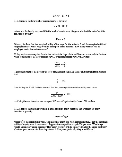
CHAPTER 1111-1. Suppose the firm’s labor demand curve is given by:w = 20 - 0.01 E ,where w is the hourly wage and E is the level of employment. Suppose also that the union’s utility function is given byU = w × E .It is easy to show that the marginal utility of the wage for the union is E and the marginal utility of employment is w . What wage would a monopoly union demand? How many workers will be employed under the union contract?Utility maximization requires the absolute value of the slope of the indifference curve equal the absolute value of the slope of the labor demand curve. For the indifference curve, we have thatEw MU MU w E =.The absolute value of the slope of the labor demand function is 0.01. Thus, utility maximization requires that01.=Ew .Substituting for E with the labor demand function, the wage that maximizes utility must solve01.0100000,2=−ww ,which implies that the union sets a wage of $10, at which price the firm hires 1,000 workers.11-2. Suppose the union in problem 1 has a different utility function. In particular, its utility function is given by:U = (w - w *) × Ewhere w * is the competitive wage. The marginal utility of a wage increase is still E , but the marginal utility of employment is now w – w *. Suppose the competitive wage is $10 per hour. What wage would a monopoly union demand? How many workers will be employed under the union contract? Contrast your answers to those in problem 1. Can you explain why they are different?Again equate the absolute value of the slope of the indifference curve to the absolute value of the slope of the labor demand curve:01.0*=−=Ew w MU MU w E .Setting w* = $10 and using the labor demand equation yields:01.0100000,210=−−ww .Thus, the union demands a wage of $15, at which price the firm hires 500 workers.In problem 1, the union maximized the total wage bill. In problem 2 the utility function depends on the difference between the union wage and the competitive wage. That is, the union maximizes its rent. Since the alternative employment pays $10, the union is willing to suffer a cut in employment in order to obtain a greater rent.11-3. Using the model of monopoly unionism, present examples of economic or political activities that the union can pursue to manipulate the firm’s elasticity of labor demand. Relate your examples to Marshall’s rules of derived demand.Marshall’s rules state that the elasticity of labor demand is lower the1. lower is the elasticity of substitution;2. lower is the elasticity of demand for the output;3. lower is labor’s share of total costs; and4. lower is the supply elasticity of other factors of production.Consider two examples: innovations and picket lines. Unions are notoriously bad at allowing firms to introduce (labor saving) innovations in their factories. The long shoremen on the west coast recently struck, because they were unwilling to let cargo crates be identified with bar codes. (The union wanted a union worker to record all movements of crates with pencil and paper.) Thus, the union was pursuing a policy of limiting the supply of other factors of production (rule 4). In a similar vein, when on strike, unions picket the firm in order to decrease the ability of the firm to hire scabs (rule 1).11-4. Suppose the union only cares about the wage and not about the level of employment. Derive the contract curve and discuss the implications of this contract curve.The utility function U = U(w) implies that the union’s indifference curves are horizontal lines, so that the contract curve coincides exactly with the firm’s labor demand curve (D).11-5. A bank has $5 million in capital that it can invest at a 5 percent annual interest rate. A group of 50 workers comes to the bank wishing to borrow the $5 million. Each worker in the group has an outside job available to him or her paying $50,000 per year. If the group of workers borrows the $5 million from the bank, however, they can set up a business (in place of working their outside jobs) that returns $3 million in addition to maintaining the original investment.(a) If the bank has all of the bargaining power (that is, the bank can make a take-it or leave-it offer), what annual interest rate will be associated with the repayment of the loan? What will be each worker’s income for the year?If the bank has all of the bargaining power, it will pay each worker exactly their reservation wage, i.e., $25,000. The total cost of this is $2.5 million. Thus, the firm will claim the remaining $500,000 by imposing a 10 percent interest rate as $500,000 is 10 percent of the original $5 million.(b) If the workers have all of the bargaining power (that is, the workers can make a take-it or leave-it offer), what annual interest rate will be associated with the repayment of the loan? What will be each worker’s income for the year?If the workers have all of the bargaining power, they will pay the bank its reservation value, i.e., an interest rate of 5 percent. When it does this, the 50 workers receive $3 million less the 5 percent interest of $250,000 for a total of $2.75 million. Split evenly among the 50 workers, this leaves each worker with a yearly income of $55,000.11-6. Consider a firm that faces a constant per unit price of $1,200 for its output. The firm hires workers, E, from a union at a daily wage of w, to produce output, q, whereq = 2E½.Given the production function, the marginal product of labor is 1/E½. There are 225 workers in the union. Any union worker who does not work for the firm can find a non-union job paying $96 per day.(a) What is the firm’s labor demand function?The labor demand function, or the marginal revenue product of labor, isMRP E = MR × MP E = 1200 / E ½.(b) If the firm is allowed to specify w and the union is then allowed to provide as many workers as it wants (up to 225) at the daily wage of w, what wage will the firm set? How many workers will the union provide? How much output will be produced? How much profit will the firm earn? What is the total income of the 225 union workers?If the firm offers w < $96, no workers will be provided. This would leave the firm with no output and no profit. The workers would all receive $96 per day, making their total daily income $21,600.If the firm offers a wage of w > $96, all 225 workers will be provided. These 225 workers would produce 30 units of output. The firm would then earn a profit of 30($1,200) – 225w. Profit, therefore, is maximized when w is minimized subject to the constraint. If the union would supply all 225 workers at a wage of $96, for example, the firm would offer w = $96 and earn a daily profit of $14,400. The total daily income of the 225 workers would remain at $21,600.If the firm needs to offer strictly more than $96 per day to attract workers, it would offer a daily wage of $96.01. All 225 workers would work for the firm, making 30 units of output. The firm’s daily profit would be $14,397.75. And the total daily income of the 225 workers would be $21,602.25.(c) If the union is allowed to specify w and the firm is then allowed to hire as many workers as it wants (up to 225) at the daily wage of w, what wage will the union set in order to maximize the total income of all 225 workers? How many workers will the firm hire? How much output will be produced? How much profit will the firm earn? What is the total income of the 225 union workers?The spreadsheet looks like the following, where the union specifies the wage, labor demand comes from part (a), and everything else follows naturally:wageLaborDemandLaborCosts Output Price Revenue ProfitUnionDaily Income$96 156.25 $15,000.00 25.00 $1,200 $30,000.00 $15,000.00 $19,200.00$97 153.04 $14,845.36 24.74 $1,200 $29,690.72 $14,845.36 $19,353.04$98 149.94 $14,693.88 24.49 $1,200 $29,387.76 $14,693.88 $19,499.88$99 146.92 $14,545.45 24.24 $1,200 $29,090.91 $14,545.45 $19,640.77$100 144.00 $14,400.00 24.00 $1,200 $28,800.00 $14,400.00 $19,776.00…… ……… … … …$190 39.89 $7,578.95 12.63 $1,200 $15,157.89 $7,578.95 $22,949.58$191 39.47 $7,539.27 12.57 $1,200 $15,078.53 $7,539.27 $22,949.90$192 39.06 $7,500.00 12.50 $1,200 $15,000.00 $7,500.00 $22,950.00$193 38.66 $7,461.14 12.44 $1,200 $14,922.28 $7,461.14 $22,949.90$194 38.26 $7,422.68 12.37 $1,200 $14,845.36 $7,422.68 $22,949.60$195 37.87 $7,384.62 12.31 $1,200 $14,769.23 $7,384.62 $22,949.11 Thus, the union sets a daily wage of $192. The firm responds by hiring 39.06 workers, who produce 12.5 units of output. The firm earns a daily profit of $7,500, while the 225 union workers earn a total of $25,297.92 each day.11-7. Suppose the union’s resistance curve is summarized by the following data. The union’s initial wage demand is $10 per hour. If a strike occurs, the wage demands change as follows:Length of Strike: Hourly Wage Demanded1 month 92 months 83 months 74 months 65 or more months 5Consider the following changes to the union resistance curve and state whether the proposed change makes a strike more likely to occur, and whether, if a strike occurs, it is a longer strike. (a) The drop in the wage demand from $10 to $5 per hour occurs within the span of 2 months, as opposed to 5 months.If the union is willing to drop its demands very fast, the firm will find it profitable to delay agreement until the wage demand drops to $5. A strike, therefore, is more likely to occur. If $5 is the lowest wage the union is willing to accept, the strike would probably last 2 months.(b) The union is willing to moderate its wage demands further after the strike has lasted for 6 months. In particular, the wage demand keeps dropping to $4 in the 6th month, $3 in the 7th month, etc.If the union is willing to accept even lower wages in the future, some firms will find it optimal to wait the union out. Thus, strikes will be more likely and last longer.(c) The union’s initial wage demand is $20 per hour, which then drops to $9 after the strike lasts one month, $8 after 2 months, and so on.Conditioning on a strike occurring, the length of strike will be unchanged as the resistance curve after the initial demand stays the same. Of course, the probability of a strike occurring increases when the initial demand increases.11-8. (a) Would you expect unions to be more willing to call a strike during good economic times or bad economics times? Explain.This is an open question – much empirical evidence suggests that strikes are procyclical – a conclusion that the model of job search supports. During good economic times, there are many good jobs available, searching for jobs is relatively easy, and the probability of securing a job is quite high. In short, the non-union option is quite attractive. During such times, therefore, the union may be a tough negotiator, and this tough stance may lead to more strikes being called. (This doesn’t explain, though, why the firms are also tough negotiators during such times.)The opposite happens during bad economic times. Namely, jobs are scarce, they are difficult to find, and searching is costly. The non-union option, therefore, is not very attractive. Consequently, the union leadership may be more willing to accept a deal. This softer stance, therefore, may lead to fewer strikes being called.(b) Does Table 627 of the 2002 U.S. Statistical Abstract provide evidence to support your answer to part (a)? What is the single overriding pattern in this table?There is some evidence that strikes are more prevalent in good times than bad (compare the 1960s to the early 1970s), but there was much more strike activity in the late 1970s and early 1980s than in the mid to late 1980s.The single most obvious pattern in the table, however, is that as union membership steadily fell over this time period, the level of strike activity also fell. The average percent or working time lost to a strike was about 12 percent, 10 percent, 4 percent, and 2 percent for the 1960s, 1970s, 1980s, and 1990s respectively.11-9. Suppose the value of the marginal product of labor in the steel industry is VMP E = 100,000 – E dollars per year, where E is the number of steel workers. The competitive wage for the workers with the skills needed in steel production is $30,000 a year, but the industry is unionized so that steel workers earn $35,000 a year. The steelworkers’ union is a monopoly union. What is the efficiency cost of the union contract in this industry?If the steel industry were to pay the competitive wage to its workers, it would employ 70,000 workers, because at this level the VMP of the last employee equals the competitive wage. Under the union wage, however, the industry only hires 65,000 workers. The efficiency cost of the union, therefore, is(½)($35,000 – $30,000)($70,000 – $65,000) = $125 million per year.11-10. Suppose the economy consists of a union and a non-union sector. The labor demand curve in each sector is given by L = 1,000,000 – 20w. The total (economy-wide) supply of labor is 1,000,000, and it does not depend upon the wage. All workers are equally skilled and equally suited for work in either sector. A monopoly union sets the wage at $30,000 in the union sector. What is the union wage gap? What is the effect of the union on the wage in the non-union sector?In a competitive economy, the wage would be the same in the two sectors, and its value would be such that the total labor demand L D = 2 × (1,000,000 – 20w C) equaled total labor supply. The solution to the equation 2 (1,000,000 – 20w C) = 1,000,000 is w C = $25,000.If the union wage is set at $30,000, the union sector employs 400,000 workers. The remaining 600,000 must be employed in the non-union sector, which will happen if the wage in the non-union sector is (1,000,000 – 600,000)/20 = $20,000.Hence, the wage gap between the union and the non-union sectors equals $10,000, or 50 percent of the non-union wage.11-11. Consider Table 628 of the 2002 U.S. Statistical Abstract.(a) How many workers were covered by a union contract in 1983? What percent of the workforce was unionized?In 1983, 20.532 million workers (23.3 percent of all workers) were covered by a union contract in the U.S.(b) How many workers were covered by a union contract in 2001? What percent of the workforce was unionized?In 2001, 17.878 million workers (14.8 percent of all workers) were covered by a union contract in the U.S.(c) Decompose the changes from part (a) to part (b) in terms of public- and private-sector workers and unions.This dramatic change in union coverage masks an even deeper pattern in union coverage – namely that public-sector unions have been growing in absolute numbers and holding their own in percent coverage, while the private-sector unions have experienced sharp decreases in their enrollments.The number of public-sector workers covered by a union contract, for example, increased from just over 7 million in 1983 to almost 8 million in 2001. The percent of public-sector workers who were members of a union held constant over this time span at roughly 37 percent, while the percent of public-sector workers covered by a union contract fell slightly from 45.5 percent in 1983 to 41.7 percent in 2001.On the other hand, the number of private-sector workers covered by a union contract decreased from 13.4 million in 1983 to only 9.9 million in 2001. The percent of private-sector workers covered by a union contract also fell drastically, from 18.5 percent in 1983 to just 9.7 percent in 2001.11-12. Consider table 618 in the 2002 U.S. Statistical Abstract.(a) Calculate the union wage effect. Calculate the union effect on total benefits. Calculate the union effect on total compensation.The union effects are simply the ratio of the union amount divided by the non-union amount:Wage effect: $19.33 / $15.38 = 1.257 percent.Benefit effect: $10.09 / $5.41 = 1.865 percentTotal compensation effect: $29.42 / $20.79 = 1.415 percent.(b) Note that for most categories, retirement and savings increases total compensation by about 60 to 80 cents per hour, with roughly two-thirds of this expense coming in defined contribution retirement plans. In contrast, retirement and savings adds $1.64 to the hourly compensation of union workers, and over 70 percent of this comes in the form of defined benefit pension plans, not defined contribution. What is the difference between defined benefit and defined contribution plans? Why might a union prefer (and be able to negotiate) more compensation in defined benefit plans than defined contribution plans?A defined benefit plan specifies the retirement benefit as a fixed dollar amount. For example, if someone receives 50 percent of their last annual income as their annual pension, this is a defined benefit plan. In contrast, a defined contribution plan specifies the amount of savings into a retirement plan the firm will make. The amount of benefit eventually received by the worker depends on how well the money is invested until retirement.It is generally thought the workers prefer DB plans (though this doesn’t need to be the case). DB plans put the risk on the part of the firm, while DC plans put the financial risk on the part of the worker. (The workers at Enron, for example, lost huge amounts of retirement savings not only because they were in a DC plan but also because they were forced to keep most of their contributions as Enron stock.) As unions tend to work in large firms, they may be more able than other workers to negotiate a DB plan.。

《劳动经济学》（作者Borjas）第四章习题答案

《劳动经济学》（作者Borjas）第四章习题答案CHAPTER 44-1. Suppose there are two inputs in the production function, labor and capital, and these two inputs are perfect substitutes. The existing technology permits 1 machine to do the work of 3 persons. The firm wants to produce 100 units of output. Suppose the price of capital is $750 per machine per week. What combination of inputs will the firm use if the weekly salary of each worker is $300? What combination of inputs will the firm use if the weekly salary of each worker is $225? What is the elasticity of labor demand as the wage falls from $300 to $225?Because labor and capital are perfect substitutes, the isoquants (in bold) are linear and the firm will use only labor or only capital, depending on which is cheaper in producing 100 units of output.The (absolute value of the) slope of the isoquant (MP E / MP K ) is 1/3 because 1 machine does the work of 3 men. When the wage is $900 (left panel), the slope of the isocost is 300/750. The isocost curve,therefore, is steeper than the isoquant, and the firm only hires capital (at point A ). When the weekly wage is $225 (right panel), the isoquant is steeper than the isocost and the firm hires only labor (at point B ).Weekly Salary = $300 Weekly Salary = $225The elasticity of labor demand is defined as the percentage change in labor divided by the percentage change in the wage. Because the demand for labor goes from 0 to a positive quantity when the wagedropped to $225, the (absolute value of the) elasticity of labor demand is infinity.LaborCapitalLaborCapital4-2. (a) What happens to the long-run demand curve for labor if the demand for the firm’s output increases?The labor demand curve is given by VMP E = MR x MP E. As demand for the firm’s output increases, its marginal revenue also increases. Thus, an increase in demand for the firm’s output shifts the labor demand curve to the right.(b) What happens to the long-run demand curve for labor if the price of capital increases?To determine how an increase in the price of capital changes the demand for labor, suppose initially that the firm is producing 200 units of output at point P in the figure. The increase in the price of capital (assuming capital is a normal input) increases the marginal costs of the firm and will reduce the profit-maximizing level of output to say 100 units. The increase in the price of capital also flattens the isocost curve, moving the firm to point R. The move from point P to point R can be decomposed into a substitution effect (P to Q) which reduces the demand for capital, but increases the demand for labor, and a scale effect (Q to R) which reduces the demand for both labor and capital. The direction of the shift in the demand curve for labor, therefore, will depend on which effect is stronger: the scale effect or the substitution effect.4-3. Union A wants to represent workers in a firm that hires 20,000 person workers when the wage rate is $4 and hires 10,000 workers when the wage rate is $5. Union B wants to represent workers in a firm that hires 30,000 workers when the wage is $6 and hires 33,000 workers when the wage is $5. Which union would be more successful in an organizing drive?The union will be more likely to attr act the workers’ support when the elasticity of labor demand (in absolute value) is small. The elasticity of labor demand facing union A is given by: η = percent ?L / percent ?w = (20,000–10,000)/20,000 ÷ (4–5)/4 = –2.The elasticity of labor demand facing union B equals (33,000–30,000)/33,000 ÷ (5–6)/5 = –5/11 ≈ –.45. Union B, therefore, is likely to have a more successful organizing drive as 0.45 < 2.4-4. Consider a firm for which production depends on two normal inputs, labor and capital, with prices w and r, respectively. Initially the firm faces market prices of w = 6 and r = 4. These prices then shift to w = 4 and r = 2.(a) In which direction will the substitution effect change the firm’s employment and capital stock?Prior to the price shift, the absolute value of the slope of the isocost line (w/r) was 1.5. After the price shift, the slope is 2. In other words, labor has become relatively more expensive than capital. As a result, there will be a substitution away from labor and towards capital (the substitution effect).(b) In which direction will the scale effect change the firm’s employment and capital stock?Because both prices fall, the marginal cost of production falls, and the firm will want to expand. The scale effect, therefore, increases the demand for both labor and capital (as both are normal inputs).(c) Can we say conclusively whether the firm will use more or less labor? More or less capital?The firm will certainly use more capital as the substitution and scale effects reinforce each other in that direction, but the change in labor employed will depend on whether the substitution or the scale effect for labor dominates.4-5. What happens to employment in a competitive firm that experiences a technology shock such that at every level of employment its output is 200 units/hour greater than before?Because output increases by the same amount at every level of employment, the marginal product of labor, and hence the value of the marginal product of labor, does not change. Therefore, as the value of the marginal product of labor will equal the wage rate at the same level of employment as before, the level of employment will not change.4-6. Suppose the market for labor is competitive and the supply curve for labor is backwardbending over part of its range. The government now imposes a minimum wage in this labor market. What is the effect of the minimum wage on employment? Does the answer depend on which of the two curves (supply or demand) is steeper? Why?Equilibrium is attained where the supply curve intersects the demand curve, and the equilibriumemployment and wage levels are E* and w*, respectively . When the minimum wage is set at w MIN , the firm wants to hire E D workers but E S workers are looking for work. As long as the downward-sloping portion of the supply curve is to the right of the demand curve, the fact that the supply curve is downward sloping creates no problems beyond those encountered in the typical competitive model. An interesting extension of the problem would consider the case where the downward-sloping portion of the supply curve recrosses the demand curve at some point above w * and the minimum wage is set above that point.4-7. Suppose a firm purchases labor in a competitive labor market and sells its product in a competitive product market. Thefirm’s elasticity of demand for labor is ?0.4. Suppose the wage increases by 5 percent. What will happen to the number of workers hired by the firm? What will happen to the marginal productivity of the last worker hired by the firm?Given the estimates of the elasticity of labor demand and the change in the wage, we have that4.0%%?=??=w E η => 4.0%5%?=?E=> %2%?=?E .Thus, the firm hires 2 percent fewer workers. Furthermore, because the labor market is competitive, the marginal worker is paid the value of his marginal product. As the product market is also competitive, therefore, we know that the output price does not change so that the marginal productivity of the marginal worker increases by 5 percent.Employment W agesw M INS D4-8. A firm’s technology requires it to combine 5 person-hours of labor with 3 machine-hours to produce 1 unit of output. The firm has 15 machines in place and the wage rate rises from $10 per hour to $20 per hour. What is the firm’s short-run elasticity of labor demand?Unless the firm goes out of business, it will combine 25 persons with the 15 machines it has in place regardless of the wage rate. Therefore, employment will not change in response to the movement of the wage rate, and the short-run elasticity of labor demand is zero.4-9. In a particular industry, labor supply is E S = 10 + w whilelabor demand is E D = 40 ? 4w, where E is the level of employment and w is the hourly wage.(a) What is the equilibrium wage and employment if the labor market is competitive? What is the unemployment rate?In equilibrium, the quantity of labor supplied equals the quantity of labor demanded, so that E S = E D. This implies that 10 + w = 40 – 4w. The wage rate that equates supply and demand is $6. When the wage is $6, 16 persons are employed. There is no unemployment because the number of persons looking for work equals the number of persons employers are willing to hire.(b) Suppose the government sets a minimum hourly wage of $8. How many workers would lose their jobs? How many additional workers would want a job at the minimum wage? What is the unemployment rate?If employers must pay a wage of $8, employers would only want to hire E D = 40 – 4(8) = 8 workers, while E S = 10 + 8 = 18 persons would like to work. Thus, 8 workers lose their job following the minimum wage and 2 additional people enter the labor force. Under the minimum wage, the unemployment rate would be 10/18, or 55.6 percent.4-10. Suppose the hourly wage is $10 and the price of each unit of capital is $25. The price of output is constant at $50 per unit. The production function isf(E,K) = E?K ?,so that the marginal product of labor isMP E = (?)(K/E) ? .If the current capital stock is fixed at 1,600 units, how much labor should the firm employ in the short run? How much profit will the firm earn?The firm’s labor demand curve is it marginal revenueproduct of labor curve, VMP E, which equals the marginal productivity of labor, MP E, times the marginal revenue of the firm’s product. Bu t as price is fixed at $50, MR = 50. Thus, we have thatVMP E = MP E× MR = (?)(1,600/E)?(50) = 1,000 / E? .Now, by setting VMP E = w and solving for E, we find that the optimal number of workers for the firm to hire is 10,000 workers. The firm then makes (1600)?(10000)? = 4,000 units of output and earns a profit of 4,000($50) – 1,600($25) – 10,000 ($10) = $60,000.4-11. Table 616 of the 2002 U.S. Statistical Abstract reports data on the nominal and real hourly minimum wage from 1960 through 2000. Under which president did the nominal minimum wage increase by the greatest dollar amount? Under what president did the real minimum wage increase by the greatest percentage?The data are:AdministrationsYear CurrentReal(2000)percentChangeNominalChange President1960 $1.00 $5.821961 $1.15 $6.621962 $1.15 $6.561963 $1.25 $7.03 20.79percent $0.25 Kennedy 1964 $1.25 $6.941965 $1.25 $6.831966 $1.25 $6.641967 $1.40 $7.221968 $1.60 $7.92 14.12percent $0.35 Johnson 1969 $1.60 $7.51 1970 $1.60 $7.101971 $1.60 $6.801972 $1.60 $6.591973 $1.60 $6.211974 $2.00 $6.99 -6.92percent $0.40 Nixon 1975 $2.10 $6.72 1976 $2.30 $6.96 3.57percent $0.20 Ford 1977 $2.30 $6.54 1978 $2.65 $7.001979 $2.90 $6.881980 $3.10 $6.48 -0.92percent $0.80 Carter 1981 $3.35 $6.35 1982 $3.35 $5.981983 $3.35 $5.791984 $3.35 $5.551985 $3.35 $5.361986 $3.35 $5.261987 $3.35 $5.081988 $3.35 $4.88 -23.15percent $0.00 Reagan 1989 $3.35 $4.65 1990 $3.80 $5.011991 $4.25 $5.371992 $4.25 $5.22 12.26percent $0.90 Bush 1993 $4.25 $5.06 1994 $4.25 $4.941995 $4.25 $4.801996 $4.75 $5.211997 $5.15 $5.531998 $5.15 $5.441999 $5.15 $5.322000 $5.15 $5.15 1.78percent $0.90 ClintonThe nominal minimum wage increased by the greatest dollar amount ($0.90) under both President Bush and President Clinton. In percentage terms, however, the real minimum wage increased by 12.26 percent during the Bush presidency, but only by 1.78 percent during the Clinton presidency. The greatest percent increase, however, came during the Kennedy presidency, when the minimum wage increased by over 20 percent.。

劳动经济学课后答案

名词解释：1、派生需求：是由阿弗里德·马歇尔在其《经济学原理》一书中首次提出的经济概念，是指对生产要素的需求，意味着它是由对该要素参与生产的产品的需求派生出来的，又称“引致需求”。

对一种生产要素的需求来自（派生自）对另一种产品的需求。

其中该生产要素对这一最终产品会作贡献，如对轮胎的需求派生自对汽车运输的需求。

1.短期：在短期内可变的生产要素只有劳动力，技术和资本都是不变生产要素。

2.长期：在长期内，劳动力和技术是可变生产要素，只有资本是不变生产要素。

3.卖方垄断企业：指企业在产品市场上市垄断者，但在劳动市场上市完全竞争。

4.买方垄断企业：是指企业劳动力市场是垄断者，而在产品市场上是完全竞争者。

5.替代效应:劳动使用量从LA降低到LB，资本使用量从KA上升到KB，即企业用资本代替了劳动。

6.规模效应:由于工资率的提高，企业使用劳动的边际成本将上升，从而导致企业生产更少的数量，产量的下降将会导致使用劳动数量的下降，图中变现为从B点到C点的移动，劳动数量随之下降。

7.互补性生产要素：当生产要素A的价格下降，数量增加时，对生产要素B的需求上升，则称生产要素A与生产要素B是互补。

8.替代性生产要素：当生产要素A的价格下降，数量增加时，生产要素B的数量下降，则生产要素A是生产要素B的替代性生产要素。

9.劳动需求的工资弹性：a)劳动需求的工资弹性是指当工资率变化一个百分率所引起的劳动需求变化的百分率的比值。

b)公式：ed ＝－(△L/L)/(△W/W)＝－(△L/△W)/(W/L)1.ed为劳动需求的工资弹性，△L和△W分别是劳动需求数量L和工资率W的变动量。

10、劳动的边际产品价值：VMP=MP•P，指的是增加额外一单位劳动要素的投入所带来的收益。

（三）1.劳动力：是人的劳动能力，即人在劳动过程中所运用的体力和智力的总和。

在现代劳动经济学体系中，劳动力又特指在一定年龄范围内，具有劳动能力和劳动要求。

劳动经济学(作者Borjas)第十章习题答案

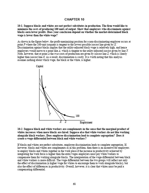
CHAPTER 1010-1. Suppose blacks and whites are not perfect substitutes in production. The firm would like to minimize the costs of producing 100 units of output. Show that employers who discriminate against blacks earn lower profits. Does your conclusion depend on whether the market-determined black wage is lower than the white wage?As drawn in the figure below, the profit-maximizing position for a non-discriminating employer occurs at point P where the 100-unit isoquant is tangent to the lowest possible isocost line given by X. Discrimination against blacks implies that the utility-adjusted black wage is relatively high, and hence employers would move to a point like A, which is tangent to the utility-adjusted isocost given by line Y. Note, however, that at point A the true costs of production are given by isocost line Z, which is clearly higher than isocost line X. As a result, discrimination is costly. It is worth noting that this analysis assumes nothing about which wage, the black or the white, is higher.Capital10-2. Suppose black and white workers are complements in the sense that the marginal product of whites increases when more blacks are hired. Suppose also that white workers do not like working alongside black workers. Does employee discrimination lead to complete segregation? Does it create a wage differential between black and white workers?If blacks and whites are perfect substitutes, employee discrimination leads to complete segregation. If, however, blacks and whites are complements as in this problem, then there is an incentive for employers to employ blacks and whites together in the work place if the increase in productivity achieved by integrating the work force is higher than the extra wages employers must pay white workers to compensate them for working alongside blacks. The interpretation of the wage differential between black and white workers is more difficult. The wage differential between the two groups will reflect not only the effect of discrimination (a higher wage for whites to encourage them to work alongside blacks), but also the effect of differences in productivity. Overall, however, it is clear that whites must be paid a compensating differential.10-3. In 1960, the proportion of blacks in Southern states was higher than the proportion of blacks in Northern states. The black-white wage ratio in Southern states was also much lower than in Northern states. Does the difference in the relative black-white wage ratios across regions indicate that Southern employers discriminated more than Northern employers?Suppose employers in neither region discriminate, so that the equilibrium black-white wage differential in both regions is determined by the (relative) demand for and supply of black workers. If there arerelatively many more black workers in the South than in the North, then the black-white wage ratio will be lower in the South than in the North, as the marginal black hired in the South is less valuable than the marginal black hired in the North. Thus, the fact that blacks earn relatively less in the South need not indicate that Southern employers discriminate more than Northern employers. Rather, the large differential may simply reflect the relatively large number of black workers in the South. (This does assume that blacks and whites are not perfect substitutes.)10-4. Suppose years of schooling, s , is the only variable that affects earnings. The equations for the weekly salaries of male and female workers are given by:w m = 500 + 100sandw f = 300 + 75s .On average, men have 14 years of schooling and women have 12 years of schooling.(a) What is the male-female wage differential in the labor market?The wage differential can be written as:∆w − = w −m – w − f = 500 + 100 s −m – ( 300 + 75 s −f ) = 500 + 100(14) – 300 – 75(12) = $700(b) Using the Oaxaca decomposition, calculate how much of this wage differential is due to discrimination?The raw wage differential is4342144443444421Skills in Difference to Due al Differenti tion Discrimina to Due al Differenti )()()(f m m f f m f m s s s w −+−+−=∆βββαα700$200$500$)1214(10012)75100()300500(Skills in Difference to Due al Differenti tion Discrimina to Due al Differenti =+=−+−+−=4342144443444421.The wage differential that is due to discrimination equals $500, or 5/7ths of the raw differential.(c) Can you think of an alternative Oaxaca decomposition that would lead to a different measure of discrimination? Which measure is better?Suppose instead of adding and subtracting βm f s to the expression giving the raw wage differential, βf m s had been added and subtracted to the expression. The Oaxaca decomposition would then be given by ∆w s s s m f m f m f m f =−+−+−()()()ααβββDifferential Due to Discrimination Differential Due to Difference in Skills 1244443444412434 700150$550$)1214(7514)75100()300500(Skills in Difference to Due al Differenti tion Discrimina to Due al Differenti =+=−+−+−=4342144443444421.Under this method, $550 of the $700 wage differential is due to discrimination. The difference between methods arises because of the way in which discrimination is defined. In one, discrimination is measured by calculating how much a woman would earn if she were treated like a man (as in the text), and in the second it is measured by calculating how much a man would earn if he were treated like a woman. On the surface, neither is a better measure. It can be shown, however, that the second approach (as in part c) attributes more variation to discrimination.10-5. Suppose the firm’s production function is given byq E E w b =+10,where E w and E b are the number of whites and blacks employed by the firm respectively. It can be shown that the marginal product of labor is thenMP E E E w b=+5.Suppose the market wage for black workers is $10, the market wage for whites is $20, and the price of each unit of output is $100.(a) How many workers would a firm hire if it does not discriminate? How much profit does this non-discriminatory firm earn if there are no other costs?There are no complementarities between the types of labor as the quantity of labor enters the production function as a sum, E w + E b . Further, the market-determined wage of black labor is less than the market-determined wage of white labor. Thus, a profit-maximizing firm will not hire any white workers and will hire black workers up to the point where the black wage equals the value of their marginal product:w p MP E b E b=×=1005()which yields E b = 2,500. The 2,500 black workers produce q = 10(sqrt(2,500)) = 500 units of output, and profits are:Π = pq – w b E b = 100(500) – 10(2,500) = $25,000.(b) Consider a firm that discriminates against blacks with a discrimination coefficient of .25. How many workers does this firm hire? How much profit does it earn?The firm acts as if the black wage is w b (1 + d ), where d is the discrimination coefficient. The employer’s hiring decision, therefore, is based on a comparison of w w and w b (1 + d ). The employer will then hire whichever input has a lower utility-adjusted price. As d = 0.25, the employer is comparing a white wage of $20 to a black (adjusted) wage of $12.50. As $12.50 < $20, the firm will hire only blacks.As before, the firm hires black workers up to the point where the utility-adjusted price of a black worker equals the value of marginal product, orbE )5(10050.12=so that E b = 1,600 workers. The 1,600 workers produces 400 units of output, and profits areΠ = 100(400) – 10(1,600) = $24,000.(c) Finally, consider a firm that has a discrimination coefficient equal to 1.25. How many workers does this firm hire? How much profit does it earn?As d = 1.25, the employer compares a white wage of $20 against a black wage of $22.50. Thus, the firm hires only whites. The firm hires white workers up to the point where the price of a white worker equals the value of marginal product:wE )5(10020=so the firm hires 625 whites, produces 250 units of output, and earns profits ofΠ = 100(250) – 20(625) = $12,500.10-6. Suppose a restaurant hires only women to wait on tables, and only men to cook the food and clean the dishes. Is this most likely to be indicative of employer, employee, consumer, or statistical discrimination?If this hiring pattern is due to discrimination at all, it is most likely due to customer discrimination. It is not employer discrimination as the employer is hiring both men and women. It is further unlikely to be statistical discrimination as an employer would likely be able to determine in a short time what would happen if women became chefs or men waited on tables. The hiring pattern could result from employee discrimination as well, but this seems unlikely as wait staff and chefs/dishwashers interact on the job.10-7. Suppose that an additional year of schooling raised wages by 7 percent in 1970, regardless of the worker’s race or ethnicity. Suppose also that the wage differential between the average white and the average Hispanic was 36 percent. Finally, assume education is the only factor that affects productivity, and the average white worker had 12 years of schooling in 1970, while the average Hispanic worker had 9 years. By 1980, the average white worker had 13 years of education, while the average Hispanic had 11 years. A year of schooling still increased earnings by 7 percent, regardless of the worker’s ethnic background, and the wage differential between the average white worker and the average Hispanic fell to 24 percent. Was there a decrease in wage discrimination during the decade? Was there a decrease in the share of the wage differential between whites and Hispanics that can be attributed to discrimination?On the basis of their education, the average white worker should have earned 21 percent more in 1970 and 14 percent more in 1980 than the average Hispanic worker. The average Hispanic worker actually received 36 percent less in 1970 and 24 percent less in 1980. Thus, in 1970, 15 percentage points can be attributed to wage discrimination, while 10 percentage points can be attributed to wage discrimination in 1980. Hence, the degree of discrimination declined from 15 to 10 percent from 1970 to 1980. On the other hand, discrimination accounted for (15/36)×100 = 41.7 percent of the 1970 differential and(10/24)×100 = 41.7 percent of the 1980 differential. Thus, there was no change in the portion due to discrimination. The two findings are not contradictory. The wage differential decreased for two reasons – less discrimination and smaller educational differences – and the two channels were equally important. Hence, despite its absolute decrease, the importance of discrimination relative to other factors was unchanged.10-8. Use Table 211 of the 2002 U.S. Statistical Abstract.(a) How much does the average female worker earn for every 1 dollar earned by the average male worker?$23,551 / $40,257 = $0.59(b) How much does the average black worker earn for every 1 dollar earned by the average white worker?$24,979 / $33,326 = $0.75.(c) How much does the average Hispanic worker earn for every 1 dollar earned by the average white worker?$22,096 / $33,326 = $0.66.10-9. Repeat each of the three comparisons in Problem 8, except now condition on education level. In other words, calculate the wage ratios separately for all workers who have not graduated high school, have only a high school degree, have a Bachelor’s degree, and have a Master’s degree. Does the degree of labor market inequality decrease or increase after conditioning on education? Why? Men & Women:No High School Degree: $12,145 / $18,855 = $0.64.High School Degree: $18,092 / $30,414 = $0.59.Bachelor’s Degree: $32,546 / $57,706 = $0.56.Master’s Degree: $42,378 / $68,367 = $0.62.Whites & Blacks:No High School Degree: $13,569 / $16,620 = $0.82.High School Degree: $20,991 / $25,270 = $0.83.Bachelor’s Degree: $37,422 / $46,894 = $0.80.Master’s Degree: $48,777 / $55,622 = $0.88.Whites & Hispanics:No High School Degree: $16,106 / $16,620 = $0.97.High School Degree: $20,704 / $25,270 = $0.82.Bachelor’s Degree: $36,212 / $46,894 = $0.77.Master’s Degree: $50,576 / $55,622 = $0.91.In every case, the wage gap closes when education attainment is taken into account except the gap stays the same between men and women with a high school degree and the gap worsens between men and women with a Bachelor’s degree.10-10. After controlling for age and education, it is found that the average woman earns $0.80 for every $1.00 earned by the average man. After controlling for occupation to control for compensating differentials (i.e., maybe men accept riskier or more stressful jobs than women, and therefore are paid more), the average woman earns $0.92 for every $1.00 earned by the average man. The conclusion is made that occupational choice reduces the wage gap 12 cents and discrimination is left to explain the remaining 8 cents.(a) Explain why discrimination may explain more than 8 cents of the 20 cent differential (and occupational choice may explain less than 12 cents of the differential).Discrimination may occur during the process of choosing an occupation (i.e., occupational crowding). As students, for example, girls may be encouraged to take a different set of courses than boys. Later, discrimination may preclude women from being hired into the higher paying occupations. Put differently, accepting the statistics at face value requires there to be wage discrimination but no employment discrimination.(b) Explain why discrimination may explain less than 8 cents of the 20 cent differential.The labor supply curve of women and men could be different, because they have different preferences when it comes to leisure and consumption. Thus, wage differences might come about to account for gender-based preferences and not discrimination. Put differently, other factors chosen by the employee, such as hours worked or work experience, have yet to be controlled for and could explain at least some of the remaining 8 cent differential.10-11. Consider a town with 10 percent blacks (and the remainder is white). Because blacks are more likely to work the night shifts, 20 percent of all cars driven in that town at night are driven by blacks. One out of every twenty people driving at night is drunk, regardless of race. Persons who are not drunk never swerve their car, but 10 percent of all drunk drivers, regardless of race, swerve their cars. On a typical night, 5,000 cars are observed by the police force.(a) What percent of blacks driving at night are driving drunk? What percent of whites driving at night are driving drunk?The percent of drivers who are drunk is identical across races – 5 percent of all drivers regardless of race are drunk.(b) Of the 5,000 cars observed, how many are driven by blacks? How many of these cars are driven by a drunk? Of the 5,000 cars observed at night, how many are driven by whites? How many of these cars are driven by a drunk? What percent of nighttime drunk drivers are black?Of the 5,000 cars driven at night, 20 percent (or 1,000) are driven by blacks. As one out of every twenty people are drunk, there are 50 black drunk drivers. Similarly, 4,000 of the cars are driven by whites, and there are 200 drunk white drivers. Thus 20 percent (50 out of 250) of the drunk drivers are black, just like20 percent of all drivers are black.(c) The police chief believes the drunk-driving problem is mainly due to black drunk drivers. He orders his policemen to pull over all swerving cars and one in every two non-swerving cars that is driven by a black person. The driver of a non-swerving car is then given a breathalyzer test that is 100 percent accurate in diagnosing drunk driving. Under this enforcement scheme, what percent of people arrested for drunk driving will be black?One-tenth of white drunk drivers will be arrested as they were swerving. This totals 20 drivers. Likewise one-tenth of black drunk drivers will be arrested as they were seen swerving. This totals 5 drivers.Of the remaining 4,975 drivers, 995 are black with 45 being drunk. As one in every two blacks is pulled over on suspicion, 22.5 additional blacks will be arrested for drunk driving as they will fail the breathalyzer test. Therefore, at the end of the night, 47.5 people will be arrested for drunk driving, 27.5 of which are black. Therefore, even though only 20 percent of all drunks are black, the percent of drunks arrested who are black is almost 50 percent (27.5/47.5).10-12. Suppose 100 men and 100 women graduate from high school. After high school, each can work in a low-skill job and earn $200,000 over his or her lifetime, or each can pay $50,000 and go to college. College graduates are given a test. If someone passes the test, he or she is hired for a high-skill job paying lifetime earnings of $300,000. Any college graduate who fails the test, however, is relegated to a low-skill job. Academic performance in high school gives each person some idea of how he or she will do on the test if they go to college. In particular, each person’s GPA, call it x, is an “ability score” ranging from 0.01 to 1.00. With probability x, the person will pass the test if he or she attends college. Upon graduating high school, there is one man with x = .01, one with x = .02, and so on up to x = 1.00. Likewise, there is one woman with x = .01, one with x = .02, and so on up to x = 1.00.(a) Persons attend college only if the expected lifetime payoff from attending college is higher than that of not attending college. Which men and which women will attend college? What is the expected pass rate of men who take the test? What is the expected pass rate of women who take the test?Both groups are identical, so the answers are identical. The expected value requirement for attending college is:$300,000 x + $200,000 (1 – x) – $50,000 > $200,000$100,000 x > $50,000x > 0.50.Thus, the 50 men and 50 women with x = .51 to x = 1.00 all go to college and take the test. The number of test takers expected to pass is then the sum of expected pass rates: .51 + .52 + … + 1.00 = 37.75. Thus, 75.5 percent (37.75 of the 50) of men and 75.5 percent of the women who take the test are expected to pass the test.(b) Suppose policymakers feel not enough women are attending college, so they take actions that reduce the cost of college for women to $10,000. Which women will now attend college? What is the expected pass rate of women who take the test?The expected value requirement for attending college for women has changed to:$300,000 x + $200,000 (1 – x) – $10,000 > $200,000$100,000 x > $10,000x > 0.10.Thus, the 90 women with x = .11 to x = 1.00 attend college and take the test. The number of female test takers expected to pass is the sum of expected pass rates: .11 + .12 + … + 1.00 = 49.95. Thus, 55.5 percent (49.95 of the 90) of the women who take the test are expected to pass the test.。

《劳动经济学》(作者Borjas)第九章习题答案

CHAPTER 99-1. Suppose a worker with an annual discount rate of 10 percent currently resides in Pennsylvania and is deciding whether to remain there or to move to Illinois. There are three work periods left in the life cycle. If the worker remains in Pennsylvania, he will earn $20,000 per year in each of the three periods. If the worker moves to Illinois, he will earn $22,000 in each of the three periods. What is the highest cost of migration that a worker is willing to incur and still make the move?The worker must compare the present value of staying in Pennsylvania to the present value of moving to Illinois. A worker will move if the present value of earnings in Illinois minus the costs of moving there exceed the present value of earnings in Pennsylvania:74.710,54$)1.1(000,201.1000,20000,202=++=PA PV and82.181,60$)1.1(000,221.1000,22000,222=++=IL PVThe worker will move, therefore, ifPV IL – C > PV PA ,where C denotes migration costs. Thus, the worker moves ifC < 60,181.82 - 54,710.74 = $5,471.089-2. Nick and Jane are married. They currently reside in Minnesota. Nick’s present value oflifetime earnings in his current employment is $300,000, and Jane’s present value is $200,000. They are contemplating moving to Texas, where each of them would earn a lifetime income of $260,000. The couple’s cost of moving is $10,000. In addition, Nick very much prefers the climate in Texas to that in Minnesota, and he figures that the change in climate is worth an additional $2,000 to him. Jane, on the other hand, prefers Minnesota’s frigid winters, so she figures she would be $2,000 worse off because of Texas’s blistering summers. Should they move to Texas?Yes. The “climatic” aspects of the move exactly balance each other, so we should not take them into account. On the monetary side, the sum of Nick’s and Jane’s lifetime present value of earnings inMinnesota is $500,000. The corresponding amount in Texas will be $520,000. The difference between the two ($20,000) exceeds the cost of moving ($10,000), so the move will make the couple jointly better off.9-3. Mickey and Minnie live in Orlando. Mickey’s net present value of lifetime earnings in Orlando is $125,000. Minnie’s net present value of lifetime earnings in Orlando is $500,000. The cost of moving to Atlanta is $25,000 per person. In Atlanta, Mickey’s net present value of lifetime earnings would be $155,000, and Minnie’s net present value of lifetime earnings would be $510,000. If Mickey and Minnie choose where to live based on their joint well-being, will they move to Atlanta? Is Mickey a tied-mover or a tied-stayer or neither? Is Minnie a tied-mover or a tied-stayer or neither?As a couple, the net present value of lifetime earnings of staying in Orlando is $500,000 + $125,000 = $625,000 and of moving to Atlanta is $510,000 + $155,000 – $50,000 = $615,000. Thus, as a couple, they would choose to stay in Orlando. Thus, there can only be a tied-stayer. (There cannot be a tied-mover, because the couple is not moving.)For Mickey, staying in Orlando is associated with a net present value of $125,000, while moving to Atlanta would yield a net present value of $155,000 – $25,000 = $130,000. So Mickey would choose to move to Atlanta. Therefore, Mickey is a tied-stayer.For Minnie, staying in Orlando is associated with a net present value of $500,000, while moving to Atlanta would yield a net present value of $510,000 –$25,000 = $485,000. So Minnie would choose to remain in Orlando. Thus, Minnie is not a tied-stayer.9-4. Suppose a worker’s skill is captured by his efficiency units of labor. The distribution of efficiency units in the population is such that worker 1 has 1 efficiency unit, worker 2 has 2 efficiency units, and so on. There are 100 workers in the population. In deciding whether to migrate to the United States, these workers compare their weekly earnings at home (w0) with their potential earnings in the United States (w1). The wage-skills relationship in each of the two countries is given by:w0 = 700 + 0.5s,andw1 = 670 + s,where s is the number of efficiency units the worker possesses.(a) Assume there are no migration costs. What is the average number of efficiency units among immigrants? Is the immigrant flow positively or negatively selected?The earnings-skills relationship in each country is illustrated in the figure below. The US line is steeper because the payoff to a unit of skills is higher in the United States. All workers who have at least 60 efficiency units will migrate to the United States. Therefore, there is positive selection and the average number of efficiency units in the immigrant flow is approximately 80 (the exact answer depends on whether the person with 60 efficiency units, who is indifferent between moving or not, moves to the United States).(b) Suppose it costs $10 to migrate to the United States. What is the average number of efficiency units among immigrants? Is the immigrant flow positively or negatively selected?If everyone incurs a cost of $10 to migrate to the United States, the U.S. wage-skill line drops by $10, and only those persons with more than 80 efficiency units will find it worthwhile to migrate. The immigrant flow is still positively selected and has, on average, 90 efficiency units.(c) What would happen to the selection that takes place if migration costs are not constant in the population, but are much higher for more skilled workers?If migration costs are much higher for skilled workers, it is possible that no skilled workers will find it worthwhile to migrate. We already know that even in the absence of migration costs no worker with fewer than 60 efficiency units finds it worthwhile to migrate. If highly skilled workers find it very costly to migrate it might be the case that there is no migration to the United States.Income700660809-5. Suppose the United States enacts legislation granting all workers, including newly arrived immigrants, a minimum income floor of y− dollars.(a) Generalize the Roy model to show how this type of welfare program influences incentive tomigrate to the United States. Ignore any issues regarding how the welfare program is to be funded.(b) Does this welfare program change the selection of the immigrant flow? In particular, are immigrants more likely to be negatively selected than in the absence of a welfare program?(c) Which types of workers, the highly skilled or the less skilled, are most likely to be attracted by the welfare program?U.S. Labor Market U.S. Labor MarketThe introduction of a wage floor in the United States (at y −) shifts the U.S. earnings-skill relationship to the bold line drawn in the figures. If the returns to skills are higher in the United States (left panel above), there are then two sets of workers who find it profitable to move: those who have very high skill levels (above s P ) as well as those workers who have very low skill levels (below s L ). In contrast, if the returns to skills are lower in the United States than in the country of origin (the right panel above), the introduction of the welfare program does not change the incentives to migrate for any worker (although the incentives of some workers would change if the wage floor was high enough). The welfare program, therefore, acts as a welfare magnet for workers originating in countries that generate “brain drains”, but not in countries where unskilled workers have incentives to migrate even in the absence of wage floors.α αL P Dollars αN y −α9-6. The immigration surplus, though seemingly small in the United States, redistributes wealth from workers to firms. Present a back-of-the-envelope calculation of the losses accruing to native workers and of the gains accruing to firms. Do these calculations help explain why some segments of society are emotional in their support of changes in immigration policy that would either increase or decrease the immigrant flow?The total loss in earnings experienced by workers in the United States is given by the rectangle w 0 B F w 1 in Figure 9-11. The area of this rectangle is given by:Loss to Native Workers = (w 1 - w 0) × N .We can calculate the loss to native workers as a fraction of GDP by dividing both sides by Q (national income). If we do this and rearrange terms we obtain:MN N Q M N w w w w Q +×+×−=)( Workers Native to Loss 0001.Thus, the native loss (as a fraction of GDP) equals the percentage change in the native wage caused by immigration times labor’s share of national income times the fraction of the labor force that is native born. If we continue the numerical example in the text, this calculation yields: (-.03) × (.7) × (.9) = -1.89percent of GDP. As national income is on the order of $11 trillion, the loss suffered by native workers is on the order of $208 billion. Capitalists receive this income plus the immigration surplus of $11 billion (see the text), for a total gain of about $219 billion (about 2 percent of GDP).Even though the net benefits from immigration are small, particular groups in the United States either gain or lose substantially from immigration. This explains why the debate over immigration policy is often polarized.9-7. In the absence of any legal barriers on immigration from Neolandia to the United States, the economic conditions in the two countries generate an immigrant flow that is negatively selected. In response, the United States enacts an immigration policy that restricts entry to Neolandians who are in the top 10 percent of Neolandia’s skill distribution. What type of Neolandian would now migrate to the United States?No one would migrate from Neolandia. The policy does not change the cost-benefit analysis for the most skilled Neolandians. They did not want to migrate when they could enter the country freely, and they still will not want to migrate when they are the only ones who can obtain visas. The lesson is that changes in immigration policy affect the skill composition of the immigrant flow only if changes target immigrants who wished to migrate to the United States in the first place.9-8. Labor demand for low-skilled workers in the United States is w = 24 – 0.1E where E is the number of workers (in millions) and w is the hourly wage. There are 120 million domestic U.S. low-skilled workers who supply labor inelastically. If the U.S. opened its borders to immigration, 20 million low-skill immigrants would enter the U.S. and supply labor inelastically. What is the market-clearing wage if immigration is not allowed? What is the market-clearing wage with open borders? How much is the immigration surplus when the U.S. opens its borders? How much surplus is transferred from domestic workers to domestic firms?Without immigration, the market-clearing wage is $12, at which all 120 million low-skill U.S. workers are employed. With immigration, the market-clearing wage is $10, at which all 120 million low-skill U.S. workers and all 20 million immigrants are employed. The additional surplus received by the U.S. because of the immigration equals ($12 – $10) (140m – 120m) / 2 = $20 million. The total transfer from U.S. workers to U.S. firms because of the immigration equals ($12 – $10) (120m) = $240 million.9-9. A country has two regions, the North and the South, which are identical in all respects except the hourly wage and the number of workers. The demand for labor in each region is:w N = $20 – .5E N and w S = $20 – .5E S,where E N and E S are millions of workers. Currently there are 6 million workers in the North and 18 million workers in the South.(a) What is the wage in each region?The wage in the North is $20 – .5 (6) = $17. The wage in the South is $20 – .5 (18) = $11.(b) If there were no shocks to the economy, migration over time will result in an equalization of wages and employment. What would be the long-run wage and employment level in each region?As labor demand is the same in both regions and workers are identical in their preferences, half of the workers will locate in each region in the long-run. Thus, 12 million workers will work in each region, and the hourly wage will be $14.(c) Return to the original set-up where there are 6 million workers in the North and 18 million workers in the South. As a policy maker, you decide not only to allow 2 million immigrants of working age to enter your country, but you have the authority to resettle the immigrants wherever you want. How should you distribute immigrants across the regions to maximize the country’s immigration surplus? Besides maximizing the immigration surplus in the short-run, in what other ways does your distribution of immigrants help the economy?Let I N and I S be the number of immigrants (in millions) placed in the North and in the South respectively, so that I N + I S = 2. After immigration, the new wages are:w N = $17 – .5I N and w S = $11 – .5I Sand the immigrant surpluses are:S N = 0.25(I N)2 and S S = .25(I S)2.Using that I N + I S = 2, therefore, the total immigrant surplus isS = 0.25(I N)2 + 0.25(2–I N)2 = 1 – I N + .5(I N)2.One can use calculus to solve for the optimal value for I N, but be aware that S is U-shaped, so setting the first order conditions to 0 solves for a minimum. Rather, use Excel to plot S. The data are:I N S I N S I N S I N S0.001.000.05 0.95 0.55 0.60 1.05 0.50 1.55 0.650.10 0.91 0.60 0.58 1.10 0.51 1.60 0.680.15 0.86 0.65 0.56 1.15 0.51 1.65 0.710.20 0.82 0.70 0.55 1.20 0.52 1.70 0.750.25 0.78 0.75 0.53 1.25 0.53 1.75 0.780.30 0.75 0.80 0.52 1.30 0.55 1.80 0.820.35 0.71 0.85 0.51 1.35 0.56 1.85 0.860.40 0.68 0.90 0.51 1.40 0.58 1.90 0.910.45 0.65 0.95 0.50 1.45 0.60 1.95 0.950.50 0.63 1.00 0.50 1.50 0.63 2.00 1.00 Thus, the immigrant surplus is maximized by placing all 2 million immigrants in either of the regions. It would be best, however, to place them all in the high wage region, as this will lead to a faster equalization of wages and saves natives the trouble and costs of moving.9-10. Phil has two periods of work remaining prior to retirement. He is currently employed in a firm that pays him the value of his marginal product, $50,000 per period. There are many other firms that Phil could potentially work for. There is a 50 percent chance of Phil being a good match for any particular firm, and a 50 percent chance of him being a bad match. If he is in a good match, the value of his marginal product is $56,000 per period. If he is in a bad match, the value of his marginal product is $40,000 per period. If Phil quits his job, he can immediately find employment with any of the alternative firms. It takes one period to discover whether Phil is a good or a bad match with a particular firm. In that first period, while Phil’s value to the firm is uncertain, he is offered a wage of $48,000. After the value of the match is determined, Phil is offered a wage equal to the value of his marginal product in that firm. When offered that wage, Phil is free to (a) accept;(b) reject and try some other firm; or (c) return to his original firm and his original wage. Phil maximizes the present value of his expected lifetime earnings, and his discount rate is 10 percent. What should Phil do?Phil makes decisions at the beginning of each period, and there are a variety of choices at each of these times. To reduce the number of strategies that require the numerical calculation of the expected outcome, first discard unreasonable choices. In particular, if Phil does not quit his job in period 1, he should not do so in period 2. After all, his second-period wage in a new job will be lower than in the old job, and there is no third period. Similarly, if he tries a new job in period 1 and is found to be a bad match, he should return to the old job. After all, the old job pays a higher wage than what Phil’s current employer is willing to pay and what another new firm would offer him. Finally, if he tries a new job and is found to be a good match, he should certainly accept their offer. In the end, Phil only has two potentially viable strategies.Strategy one: Keep the old job in both periods. The earnings path associated with this choice is flat and deterministic – Phil earns $50,000 in each period. The present discounted value of the outcome of this strategy is PV1 = 50,000 + 50,000/1.1 = $95,455.Strategy two: Try a new job. If it is a good match, keep it. If it is a bad match, return to the old job. If Phil adopts this strategy, he will earn $48,000 in period 1. In period 2, he will earn either $56,000 or $50,000, each with probability ½. The expected present discounted value of the outcome of that strategy is PV2 = 48,000 + ((½× 56,000) + (½ × 50,000))/1.1 = $96,182.As the second strategy generates a higher present value, this is the strategy Phil adopts.9-11. Under the recently enacted 2001 tax legislation in the United States, all income tax filers can now deduct from their total income half of their expenses incurred when moving more than 50 miles to accept a new job. Prior to the change, only tax filers who itemized their deductions were allowed to deduct their moving expenses. (Typically, homeowners itemize their deductions and renters do not itemize.) How would this change in the tax bill likely affect the mobility of homeowners and renters?The policy change has no affect on homeowners, whereas the policy change reduces the cost of moving for renters. Therefore, the policy is predicted to increase the mobility of renters.。

《劳动经济学》(作者Borjas)第五章习题答案

CHAPTER 55-1. Suppose the labor supply curve is upward sloping and the labor demand curve is downward sloping. The study of economic trends over a particular time period reveals that the wage recently fell while employment levels rose. Which curve must have shifted and in which direction to produce this effect?If the supply curve does not shift, all wage and employment movements must occur along the supply curve, so that the wage rate and the employment level must move in the same direction. Because the wage went down while employment went up in the situation described in the question, it must have been the case that the supply curve shifted outwards (to the right). We do not have enough information to determine whether the demand curve shifted as well.5-2. It takes time to produce a new economist, and prospective economists base their career decision by looking only at current wages across various professions. Further, the labor supply curve of economists is much more elastic than the labor demand curve. Suppose the market is now in equilibrium, but that the demand for economists suddenly rises because a new activist government in Washington wants to initiate many new programs that require the input of economists. Illustrate the trend in the employment and wages of economists as the market adjusts to this increase in demand.Initially, the market is in equilibrium at a wage w0 and an employment level of E0. The increase the demand for economists results in a new equilibrium wage of w1 and a new equilibrium employment level of E1. However, the demand for economists in the short-run is inelastic at E0, so the demand increase simply leads to a rise in the wage of economists (as indicated by point 1). In the next period, students believe this wage will persist and oversupply the market so that the cobweb leads to a new wage at point 2. In the next period, students undersupply (because the wage is too low) and the cobweb leads to a new wage at point 3, and so on. Because of the relative elasticities of supply and demand (as drawn), the cobweb is exploding and will never converge to a stable equilibrium.5-3. Suppose the supply curve of physicists is given by w = 10 + 5E , while the demand curve is given by w = 50 – 3E . Calculate the equilibrium wage and employment level. Suppose now that the demand for physicists increases and the new demand curve is given by w = 70 – 3E . Assume this market is subject to cobwebs. Calculate the wage and employment level in each round as the wage and employment levels adjust to the demand shock. (Recall that each round occurs on the demand curve – when the firm posts a wage and hires workers). What is the new equilibrium wage and employment level?The initial equilibrium is given by 10 + 5E = 50 – 3E . Solving these two equations simultaneously implies that w = $35 and E S = E D = 5. When demand increases to w = 70 – 3E , the new equilibrium wage is $47.5 and the equilibrium level of employment is 7.5.Round Wage Employment1 $55.0 52 $43.0 93 $50.2 6.64 $45.9 8.05 $48.4 7.26 $46.9 7.77 $47.8 7.48 $47.2 7.6The table gives the values for the wage and employment levels in each round. The values in the table are calculated by noting that in any given period the number of physicists is inelastically supplied, so that the wage is determined by the demand curve. Given this wage, the number of economists available in the next period is calculated. By round 7, the market wage rate is within 30 cents of the new equilibrium.01 w 1w 0W age5-4. The 1986 Immigration Reform and Control Act (IRCA) made it illegal for employers in the United States to knowingly hire illegal aliens. The legislation, however, has not reduced the flow of illegal aliens into the country. As a result, it has been proposed that the penalties against employers who break the law be increased substantially. Suppose that illegal aliens, who tend to be less skilled workers, are complements with native workers. What will happen to the wage of native workers if the penalties for hiring illegal aliens increase?A substantial increase in the penalties associated with hiring illegal aliens will likely reduce the number of illegal aliens entering the United States. The effect of this shift in the size of the illegal alien flow on the marginal product (and hence the demand curve) of native workers hinges on whether illegal aliens are substitutes or complements with natives. As it is assumed that natives and illegal aliens are complements, a cut in the number of illegal aliens reduces the value of the marginal product of natives, shifting down the demand for native labor, and decreasing native wages and employment.5-5. Suppose a firm is a perfectly discriminating monopsonist. The government imposes a minimum wage on this market. What happens to wages and employment?A perfectly discriminating monopsonist faces a marginal cost of labor curve that is identical to the supply curve. As a result, the employment level of a perfectly discriminating monopsonist equals theemployment level that would be observed in a competitive market (at E *) The imposition of a minimum wage at w MIN leads to the same result as in a competitive market: the firm will only want to hire E D workers as w MIN is now the marginal cost of labor, but E S workers will want to find work at the minimum wage. Thus, the wage increases, but employment falls.DollarsE w w *S D5-6. What happens to wages and employment if the government imposes a payroll tax on amonopsonist? Compare the response in the monopsonistic market to the response that would have been observed in a competitive labor market.Initially, the monopsonist hires E M workers at a wage of w M . The imposition of a payroll tax shifts the demand curve to VMP ′, and lowers employment to E ′ and the wage to w ′. Thus, the effect of imposing a payroll tax on a monopsonist is qualitatively the same as imposing a payroll tax in a competitive labor market: lower wages and employment. (It is interesting to note that the same result comes about if the payroll tax is placed on workers, so that the labor supply and marginal cost of labor curves shift as opposed to labor demand.)5-7. An economy consists of two regions, the North and the South. The short-run elasticity of labor demand in each region is –0.5. The within-region labor supply is perfectly inelastic. The labormarket is initially in an economy-wide equilibrium, with 600,000 people employed in the North and 400,000 in the South at the wage of $15 per hour. Suddenly, 20,000 people immigrate from abroad and initially settle in the South. They possess the same skills as the native residents and also supply their labor inelastically.(a) What will be the effect of this immigration on wages in each of the regions in the short run (before any migration between the North and the South occurs)?There will be no effect on the North’s labor supply in the short run, so the wage rate will not change there. In the South, labor supply will have increased by 5 percent, so the wage rate must fall by 5/(0.5) = 10 percent (recall that the elasticity of labor demand is -0.5, so a one percent decrease in wages would have been generated by a 0.5 percent expansion of the labor supply). The new hourly wage in the South, therefore, is $13.50 and total employment in the South is 420,000.DollarsEmploymentw M w ′(b) Suppose 1,000 native-born persons per year migrate from the South to the North in response to every dollar differential in the hourly wage between the two regions. What will be the ratio of wages in the two regions after the first year native labor responds to the entry of the immigrants?After the initial migration, we have seen that wages in the South are $13.50 while wages in the North are $15. This difference leads 1,500 natives migrating from the South to the North in the first year. Employment in the North after one year, therefore is 601,500. Moreover, as the elasticity of labor demand in the North is -0.5 and employment has increased by 0.25 percent, the Northern wage falls by 0.5 percent to roughly $14.93. Likewise, employment in the South after one year is 418,500. As the elasticity of labor demand is -0.5 and employment has decreased by 0.3571 percent, the Southern wage increases by0.71428 percent to roughly $13.60. Thus, the ratio of the Northern to Southern wage after one year is1.09779.(c) What will be the effect of this immigration on wages and employment in each of the regions in the long run (after native workers respond by moving across regions to take advantage of whatever wage differentials may exist)? Assume labor demand does not change in either region.In the long run, people must move from the South to the North to equalize the wage rates in the two regions. Since the wages were equal in the two regions before the influx of immigrants, and they also must be equal after things settle down, the proportional decrease in the wage rate should be the same in the North and in the South. Because the elasticity of labor demand is the same in the two regions, this last observation implies that the percentage increase in employment in the North must be the same as the percentage increase in employment in the South. Thus, as 60 percent of the original workers were employed in the North, 60 percent of the 20,000 increase in Southern employment will eventually migrate to the North. In the long run, therefore, total Northern employment will be 612,000 while total Southern employment will be 408,000. (Note: there is no presumption that only immigrants further migrate to the North.) In each region, therefore, employment increases by 2 percent in the long run, i.e., 12,000 is 2 percent of 600,000 and 8,000 is 2 percent of 400,000. (This can also be seen immediately as 20,000 is 2 percent of the 1 million workers.) Now, given that the elasticity of labor demand is -0.5, the 2 percent increase in employment will cause the wage rate to fall by 4 percent. Hence, the long-run equilibrium hourly wage will be $14.40.5-8. Chicken Hut faces perfectly elastic demand for chicken dinners at a price of $6 per dinner. The Hut also faces an upward sloped labor supply curve ofE = 20w – 120,where E is the number of workers hired each hour and w is the hourly wage rate. Thus, the Hut faces an upward sloped marginal cost of labor curve ofMC E = 6 + 0.1E.Each hour of labor produces 5 dinners. (The cost of each chicken is $0 as the Hut receives two-day old chickens from Hormel for free.) How many workers should Chicken Hut hire each hour to maximize profits? What wage will Chicken Hut pay? What are Chicken Hut’s hourly profits?First, solve for the labor demand curve: VMP E = P x MP E = $6 x 5 = $30. Thus, every worker is valued at $30 per hour by Chicken Hut. Now, setting VMP E = MC E yields 30 = 6 + .1E which implies E* = 240. Thus, Chicken Hut will hire 240 workers every hour. Further, according to the labor supply curve, 240 workers can be hired at an hourly wage of $18. Finally, Chicken Hut’s profits are Π = 240(5)($6) –240($18) = $2,880.5-9. Polly’s Pet Store has a local monopoly on the grooming of dogs. The daily inverse demand curve for pet grooming is:P = 20 – 0.1Qwhere P is the price of each grooming and Q is the number of groomings given each day. This implies that Polly’s marginal revenue is:MR = 20 – 0.2Q.Each worker Polly hires can groom 20 dogs each day. What is Polly’s labor demand curve as a function of w, the daily wage that Polly takes as given?As each worker can groom 20 dogs each day, and using Q = 20E, we have thatVMP E = MR x MP E = ( 20 – 0.2Q ) (20) = (20 – 4E)(20) = 400 – 80E.Thus, as Polly’s demand for labor satisfies VMP E = w, we have that her labor demand curve isE = 5 – 0.0125w.5-10. The Key West Parrot Shop has a monopoly on the sale of parrot souvenir caps in Key West. The inverse demand curve for caps is:P = 30 – 0.4 Qwhere P is the price of a cap and Q is the number of caps sold per hour. Thus, the marginal revenue for the Parrot Shop is:MR = 30 – 0.8Q.The Parrot Shop is the only employer in town, and faces an hourly supply of labor given by:w = 0.9E + 5where w is the hourly wage rate and E is the number of workers hired each hour. The marginal cost associated with hiring E workers, therefore, is:MC E = 1.8E + 5.Each worker produces two caps per hour. How many workers should the Parrot Shop hire each hour to maximize its profit? What wage will it pay? How much will it charge for each cap?First, as Q = 2E, the labor demand curve isVMP E = MR x MP E = (30 – 0.8Q)(2) = 60 – 1.6Q = 60 – 3.2E.Setting VMP E equal to MC E and solving for E yields E = 11. Eleven workers can be hired at a wage of.9(11) + 5 = $14.99 per hour. The 11 workers make 22 caps each hour, and the 22 caps can be sold at a price of 30 – 0.4(22) = $21.20 each.5-11. Ann owns a lawn mowing company. She has 400 lawns she needs to cut each week. Her weekly revenue from these 400 lawns is $20,000. If given an 18-inch deck push mower, a low-skill worker can cut each lawn in two hours. If given a 60-inch deck riding mower, a low-skill worker can cut the lawn in 30 minutes. Low-skilled labor is supplied inelastically at $5.00 per hour. Each laborer works 8 hours a day and 5 days each week.(a) If Ann decides to have her workers use push mowers, how many push mowers will Ann rent and how many workers will she hire?As each worker can cut a lawn in 2 hours, it follows that each worker can cut 4 lawns in a day or 20 lawns in a week. Therefore, Ann would need to rent 20 push mowers and hire 20 workers in order to cut all 400 lawns each week.(b) If she decides to have her workers use riding mowers, how many riding mowers will Ann rent and how many workers will she hire?As each worker can cut a lawn in 30 minutes, it follows that each worker can cut 16 lawns in a day or 80 lawns in a week. Therefore, Ann would need to rent 5 riding mowers and hire 5 workers in order to cut all 400 lawns each week.(c) Suppose the weekly rental cost (including gas and maintenance) for each push mower is $250 and the weekly rental cost (including gas and maintenance) of each riding mower is $1,800. What equipment will Ann rent? How many workers will she employ? How much profit will she earn?If Ann uses push mowers, her weekly cost of mowers is $250(20) = $5,000 while her weekly labor cost is $5(20)(40) = $4,000. Under this scenario, her weekly profit is $11,000. If Ann uses riding mowers, her weekly cost of mowers is $1,800(5) = $9,000 while her weekly labor cost is $5(5)(40) = $1,000. Thus, under this scenario, her weekly profit is $10,000. Therefore, under these conditions, Ann will rent 20 push mowers and employ 20 low-skill workers.(d) Suppose the government imposes a 20 percent payroll tax (paid by employers) on all labor and offers a 20 percent subsidy on the rental cost of capital. What equipment will Ann rent? How many workers will she employ? How much profit will she earn?Under these conditions, the cost of labor has increased to $6.00 per hour, while the rental costs for a push mower and a riding mower have decreased to $200 and $1,440 respectively. Ann’s profits under the two options, therefore, arePush-Profit = $20,000 – $200(20) – $6(20)(40) = $11,200.Rider-Profit = $20,000 – $1,440(5) – $6(5)(40) = $11,600.Thus, under these conditions, Ann rents riding mowers, hires 5 low-skill workers, and earns a weekly profit of $11,600.5-12. In the United States, some medical procedures can only be administered to a patient by a doctor while other procedures can be administered by a doctor, nurse, or lab technician. What might be the medical reasons for this? What might be the economic reasons for this?The American Medical Association might argue that doctors have more training and experience than nurses, and therefore, are the only professionals who can make certain decisions or perform certain procedures.Economically, the AMA has an incentive to restrict the number of people who can practice medicine (or perform certain procedures) in order to keep doctor wages high. If nurses were allowed to do everything they were capable of, fewer doctors would be demanded, and doctor wages would fall. From an economic viewpoint, therefore, the AMA restricts the supply of doctors, which keeps doctor wages artificially high.WageW restW unrestRestricted Supply ofDoctorsUnrestricted Supplyof DoctorsL rest L unrest Services Provided by DoctorsLabor Market For Medical Services Provided by Doctors。

《劳动经济学》(作者Borjas)第十二章习题答案

CHAPTER 1212-1. Suppose there are 100 workers in an economy with two firms. All workers are worth $35 per hour to firm A but differ in their productivity at firm B. Worker 1 has a value of marginal product of $1 per hour at firm B; worker 2 has a value of marginal product of $2 per hour at firm B, and so on. Firm A pays its workers a time-rate of $35 per hour, while firm B pays its workers a piece rate. How will the workers sort themselves across firms? Suppose a decrease in demand for both firms’ output reduces the value of every worker to either firm by half. How will workers now sort themselves across firms?Workers 1 to 34 work for firm A as a time rate of $35 is more than their value to firm B, while workers 36 to 100 work for firm B. Worker 35 is indifferent. More productive workers, therefore, flock to the piece rate firm. After the price of output falls, firm A values all workers at $17.50 per hour, while worker 1’s value at firm B falls to 50 cents, worker 2’s value falls to $1 at firm B, etc. The key question is what happens to the wage in the time-rate firm. Presumably this wage will also fall by half to $17.50 per hour. If it falls by half, then the sorting of workers to the two firms remains unchanged.12-2. Taxicab companies in the United States typically own a large number of cabs and licenses; taxicab drivers then pay a daily fee to the owner to lease a cab for the day. In return, the drivers keep their fares (so that, in essence, they receive a 100 percent commission on their sales). Why did this type of compensation system develop in the taxicab industry?Imagine what would happen if the cab company paid a 50 percent commission on fares. The cab drivers would have an incentive to misinform the company about the amount of fares they generated in order to pocket most of the receipts. Because cab companies find it almost impossible to monitor their workers, they have developed a compensation scheme that leaves the monitoring to the drivers. By charging drivers a rental fee and letting the drivers keep all the fares, each driver has an incentive to not shirk on the job.12-3. A firm hires two workers to assemble bicycles. The firm values each assembly at $12. Charlie’s marginal cost of allocating effort to the production process is MC = 4N, where N is the number of bicycles assembled per hour. Donna’s marginal cost is MC = 6N.(a) If the firm pays piece rates, what will be each worker’s hourly wage?As the firm values each assembly at $12, it will pay $12 for 1 assembly, $24 for 2 assembly’s, etc. when offering piece rates. As Charlie’s marginal cost of the first assembly is $4, the second is $8, the third is $12, and the fourth is $16; Charlie assembles 3 bicycles each hour and is paid an hourly wage of $36. Likewise, as Donna’s marginal cost of the first assembly is $6, the second is $12, and the third is $18; Donna assembles 2 bicycles each hour and is paid an hourly wage of $24.(b) Suppose the firm pays a time rate of $15 per hour and fires any worker who does not assemble at least 1.5 bicycles per hour. How many bicycles will each worker assemble in an 8 hour day?As working is painful to workers, each will work as hard as necessary to prevent being fired, but that is all. Thus, each worker assembles 1.5 bicycles each hour, for a total of 12 bicycles in an eight hour day. 12-4. All workers start working for a particular firm when they are 20 years old. The value of each worker’s marginal product is $18 per hour. In order to prevent shirking on the job, a delayed-compensation scheme is imposed. In particular, the wage level at every level of seniority is determined by:Wage = $10 + (.4 × Years in the firm).Suppose also that the discount rate is zero for all workers. What will be the mandatory retirement age under the compensation scheme? (Hint: Use a spreadsheet.)To simplify the problem, suppose the workers works 1 hour per year. (The answer would be the same regardless of how many hours are worked, as long as the number of hours worked does not change over time). Some of the relevant quantities required to determine the optimal length of the contract are:Age Yearson theJob VMPAccumulatedVMPContractWageAccumulatedContractWage21 1 $18 $18 $10.00 $10.0022 2 $18$36 $10.40 $20.4023 3 $18$54 $10.80 $31.2024 4 $18$72 $11.20 $42.4040 20 $18$360 $17.60 $276.0041 21 $18$378 $18.00 $294.0042 22 $18$396 $18.40 $312.4043 23 $18$414 $18.80 $331.2060 40 $18$720 $25.60 $712.0061 41 $18$738 $26.00 $738.0062 42 $18$756 $26.40 $764.40The VMP is constant at $18 per year. The accumulated VMP gives the total product the worker has contributed to the firm up to that point in the contract. The wage in the contract follows from the equation, and the accumulated wage is the total wage payments received by the worker up to that point. Until the 20th year in the firm, the worker receives a wage lower than her VMP; after the 21st year the worker’s wage exceeds the VMP. The contract will be terminated when the total accumulated VMP equals the total accumulated wage under the delayed compensation contract, which occurs on the worker’s 41st year on the job. So the optimal retirement age is age 61.12-5. Suppose a firm’s technology requires it to hire 100 workers regardless of the wage level. The firm, however, has found that worker productivity is greatly affected by its wage. The historical relationship between the wage level and the firm’s output is given by:Wage Rate Units of Output$8.00 65$10.00 80$11.25 90$12.00 97$12.50 102What wage level should a profit-maximizing firm choose? What happens to the efficiency wage if there is an increase in the demand for the firm’s output?The data in the problem can be used to calculate the elasticity of the change in output with respect to the change in the wage. The efficiency wage is determined by the condition that this elasticity must equal 1. This elasticity is 1 when the firm raises the wage from $10 to $11.25 an hour: (90-80)/80 ÷ (11.25-10)/10 = 1. The efficiency wage, therefore, is $11.25. Note that this efficiency wage is independent of any labor market conditions, and particularly does not depend on the demand for the firm’s output.12-6. Consider three firms identical in all aspects except their monitoring efficiency, which cannot be changed. Even though the cost of monitoring is the same across the three firms, shirkers at Firm A are identified almost for certain; shirkers at Firm B have a slightly greater chance of not being found out; and shirkers at Firm C have the greatest chance of not being identified as a shirker. If all three firms pay efficiency wages to keep their workers from shirking, which firm will pay the greatest efficiency wage? Which firm will pay the smallest efficiency wage?In this example, there is no connection between the cost of monitoring and the efficiency of monitoring. Moreover, the value of unemployment is the same for workers regardless of their employer. Focusing just on the probability of being caught shirking, therefore, workers in Firm A have the least incentive to shirk (as they are most likely to get caught) while workers in Firm C have the greatest incentive to shirk (as they are least likely to get caught). The idea of efficiency wages is to use wages to buy-off the incentive to shirk. Therefore, Firm A will pay the lowest efficiency wage, while Firm C will pay the greatest efficiency wage.12-7. Consider three firms identical in all aspects (including the probability with which they discover a shirker), except that monitoring costs vary across the firms. Monitoring workers is very expensive at Firm A, less expensive at Firm B, and cheapest at Firm C. If all three firms pay efficiency wages to keep their workers from shirking, which firm will pay the greatest efficiency wage? Which firm will pay the smallest efficiency wage?In this example, there is no connection between the cost of monitoring and the efficiency of monitoring. The efficiency wage, therefore, is determined by the incentives of the workers, not the costs of the firms. (The decision of whether to monitor workers, of course, will depend on the cost of monitoring.) Thus, all three firms will offer the same efficiency wage.12-8. Why will a firm be more likely to pay its factory workers according to a time rate, but be more likely to pay its sales people a piece rate?Each factory worker has a place on an assembly line and must do a certain task for each unit of theproduct made. Thus, the production process requires very little monitoring of workers, as they are more or less forced to do their job or else the assembly line will breakdown, with the factory manager knowing who is at fault. This is the ideal situation in which to pay a time rate.In comparison, sales persons are likely paid a piece rate, because monitoring their efforts is much more difficult. By paying a piece rate, the sales people have an incentive to work hard to make as many sales as possible.12-9. Suppose a worker only cares about her wage (a “good”) and how much effort she exerts on the job (a “bad”). Graph some indifference curves over these two goods for the worker.With the wage on the horizontal axis, any shaped indifference curves as long as they are upward sloping and increasing in the direction of higher wages and less effort fulfill the requirements that wages are a good thing and effort is a bad thing.12-10. Why would a firm ever choose to offer profit-sharing to its employees in place of paying piece rates?Piece rates can be very difficult to pay in some situations. For example, in a situation in which a group of workers is responsible for producing the good, determining who made what may be impossible. Consider Southwest Airlines, which is known to have a wonderful profit sharing program. To pay a flight attendant a piece rate, the airline would have to survey passengers as they depart the plane, and then, from the passengers’ opinions, pay the appropriate piece rates. Clearly this is unreasonable. Profit sharing, on the other hand, is a convenient way to approximate the piece rate system. Since all workers are covered by profit sharing at Southwest Airlines, all workers have a continuous incentive to do their job very well. EffortWageIndifference Curves: Wages and Effort12-11. Describe the free riding problem in a profit-sharing compensation scheme. How might the workers of a firm “solve” the free riding problem?When all workers are covered by a profit sharing plan, an individual worker has the incentive to shirk his responsibilities as his direct effect on profits is tiny. If all workers do this, however, the total profit created by the firm will be much smaller than it would be if workers were paid a piece rate.One way to “solve” the free rider problem is with social pressure. If the atmosphere of the workers is that everyone works and shirkers will be punished somehow – socially, annual reviews, being fired, etc. – then the incentive to shirk is diminished.。

劳动经济学鲍哈斯7e答案

劳动经济学鲍哈斯7e答案一、单项选择题:本大题共20小题，每小題1分，共20分。

在每小题列出的备选项中只有一项是最符合题目要求的，请将其选出。

1.劳动经济学是经济学的重要分支，主要研究A.劳动生产率B.劳动的人C.劳动资料D.劳动要素2.当劳动力供给弹生等于1时，该劳动力供给弹性为A.供给无限弹性B.单位供给弹性C.供给无弹性D.供给缺乏弹性3.妻子选择就业还是闲暇的尺度是A.家庭人口B.爱好C.家务的多少D.工资率的高低4.在工资率保持不变的情况下，由于收入的变化引起的工作时间的变化称为A.替代效应B.收入效应C.规模效应D.均衡效应5.在市场经济中，劳动力供给的决策主体是A.劳动者家庭或个人B.政府或公共部门C行业工会D.企业或雇主6.衡量社会劳动力供给总量的主要指标是A.就业率B.失业率C.劳动力供给弹性D.劳动力参与率7.如果企业雇工水平变动的百分比大于工资率变动的百分比，则此时劳动力需求弹性A.等于0B.小于1C.等于1D.大于18.如果劳动力市场上的工资率无论如何变化都不会对劳动力需求量产生任何影响，则该劳动力需求曲线(工资率为纵轴，劳动力需求量为横轴)是一条A.与横轴垂直的线B.与横轴平行的线C.向右上倾斜且较为平坦的曲线D.向右上倾斜且较为能峭的曲线9.劳动力资源能实现最优分配是在A.劳动力市场实现均衡时B.劳动力市场偏离均衡时C.当生产效率高的行业向生产效率低的行业转移劳动力时D.不同行业出现不同的工资率时10.下列选项中，关于劳动力流动说法不正确的是A.年龄越大，流动的意愿越少B.未婚比已婚容易流动C.学历越高，越可能流动D.流动的可能性与迁移距离成同方向变动11.以下属于教育间接成本的是A.老师工资B.书本费用C.学费D.不上学参加工作所得的收入12.劳动报酬的基本形式是A.直接工资和间接工资B.超额工资和累计工资C.计时工资和计件工资D.包工工资和提成工资13.工资既可以反映劳动者向社会提供的劳动贡献，也可以反映出劳动者的清费水平，这是工资的A.保障职能B.调节职能C.增值职能D.统计和监督职能14.影响宏观工资水平的主要因素是A经济效益B.劳动力分配C.工资分配形式D.物价变动15.将工人工资按照形组或个人营业额、毛利或纯收入等的定比例提取进行计发的工资形式称为A.超额计件工资B.提成工资C.集体计件工资D.累计计件工资16.知识员工通过技术股份获得收益的具体模式不包括A.技术骨干股模式B.分红回填模式C.分红股模式D.一揽子型模式17.绝大多数经济学家认为，充分就业的数量标准是失业率控制在A0-1%之间B.3-4%之间C.8-10%之间D.10-15%之间18.现在我国对女性失业者的年龄上限规定为A60B.50C.65D.5519.因为产品需求下降使厂商销售发生困难，从而对劳动供给的数量产生限制而造成的劳动者失业的现象称为A.非自愿失业B.摩擦性失业C.自愿失业D.结构性失业20.社会保障的资金来源于各要素所有名的贡献，体现了社会保障的A.保证性B.福利性C.普遍性D.互济性二、填空题:本大题共5小题，每小题2分，共10分。

《劳动经济学》(作者Borjas)第四章习题答案

CHAPTER 44-1. Suppose there are two inputs in the production function, labor and capital, and these two inputs are perfect substitutes. The existing technology permits 1 machine to do the work of 3 persons. The firm wants to produce 100 units of output. Suppose the price of capital is $750 per machine per week. What combination of inputs will the firm use if the weekly salary of each worker is $300? What combination of inputs will the firm use if the weekly salary of each worker is $225? What is the elasticity of labor demand as the wage falls from $300 to $225?Because labor and capital are perfect substitutes, the isoquants (in bold) are linear and the firm will use only labor or only capital, depending on which is cheaper in producing 100 units of output.The (absolute value of the) slope of the isoquant (MP E / MP K ) is 1/3 because 1 machine does the work of 3 men. When the wage is $900 (left panel), the slope of the isocost is 300/750. The isocost curve,therefore, is steeper than the isoquant, and the firm only hires capital (at point A ). When the weekly wage is $225 (right panel), the isoquant is steeper than the isocost and the firm hires only labor (at point B ).Weekly Salary = $300 Weekly Salary = $225The elasticity of labor demand is defined as the percentage change in labor divided by the percentage change in the wage. Because the demand for labor goes from 0 to a positive quantity when the wagedropped to $225, the (absolute value of the) elasticity of labor demand is infinity.LaborCapitalLaborCapital4-2. (a) What happens to the long-run demand curve for labor if the demand for the firm’s output increases?The labor demand curve is given by VMP E = MR x MP E. As demand for the firm’s output increases, its marginal revenue also increases. Thus, an increase in demand for the firm’s output shifts the labor demand curve to the right.(b) What happens to the long-run demand curve for labor if the price of capital increases?To determine how an increase in the price of capital changes the demand for labor, suppose initially that the firm is producing 200 units of output at point P in the figure. The increase in the price of capital (assuming capital is a normal input) increases the marginal costs of the firm and will reduce the profit-maximizing level of output to say 100 units. The increase in the price of capital also flattens the isocost curve, moving the firm to point R. The move from point P to point R can be decomposed into a substitution effect (P to Q) which reduces the demand for capital, but increases the demand for labor, and a scale effect (Q to R) which reduces the demand for both labor and capital. The direction of the shift in the demand curve for labor, therefore, will depend on which effect is stronger: the scale effect or the substitution effect.4-3. Union A wants to represent workers in a firm that hires 20,000 person workers when the wage rate is $4 and hires 10,000 workers when the wage rate is $5. Union B wants to represent workers in a firm that hires 30,000 workers when the wage is $6 and hires 33,000 workers when the wage is $5. Which union would be more successful in an organizing drive?The union will be more likely to attract the workers’ support when the elasticity of labor demand (in absolute value) is small. The elasticity of labor demand facing union A is given by:η = percent ∆L / percent ∆w = (20,000–10,000)/20,000 ÷ (4–5)/4 = –2.The elasticity of labor demand facing union B equals (33,000–30,000)/33,000 ÷ (5–6)/5 = –5/11 ≈ –.45. Union B, therefore, is likely to have a more successful organizing drive as 0.45 < 2.4-4. Consider a firm for which production depends on two normal inputs, labor and capital, with prices w and r, respectively. Initially the firm faces market prices of w = 6 and r = 4. These prices then shift to w = 4 and r = 2.(a) In which direction will the substitution effect change the firm’s employment and capital stock?Prior to the price shift, the absolute value of the slope of the isocost line (w/r) was 1.5. After the price shift, the slope is 2. In other words, labor has become relatively more expensive than capital. As a result, there will be a substitution away from labor and towards capital (the substitution effect).(b) In which direction will the scale effect change the firm’s employment and capital stock?Because both prices fall, the marginal cost of production falls, and the firm will want to expand. The scale effect, therefore, increases the demand for both labor and capital (as both are normal inputs).(c) Can we say conclusively whether the firm will use more or less labor? More or less capital?The firm will certainly use more capital as the substitution and scale effects reinforce each other in that direction, but the change in labor employed will depend on whether the substitution or the scale effect for labor dominates.4-5. What happens to employment in a competitive firm that experiences a technology shock such that at every level of employment its output is 200 units/hour greater than before?Because output increases by the same amount at every level of employment, the marginal product of labor, and hence the value of the marginal product of labor, does not change. Therefore, as the value of the marginal product of labor will equal the wage rate at the same level of employment as before, the level of employment will not change.4-6. Suppose the market for labor is competitive and the supply curve for labor is backwardbending over part of its range. The government now imposes a minimum wage in this labor market. What is the effect of the minimum wage on employment? Does the answer depend on which of the two curves (supply or demand) is steeper? Why?Equilibrium is attained where the supply curve intersects the demand curve, and the equilibriumemployment and wage levels are E* and w*, respectively . When the minimum wage is set at w MIN , the firm wants to hire E D workers but E S workers are looking for work. As long as the downward-sloping portion of the supply curve is to the right of the demand curve, the fact that the supply curve is downward sloping creates no problems beyond those encountered in the typical competitive model. An interesting extension of the problem would consider the case where the downward-sloping portion of the supply curve recrosses the demand curve at some point above w * and the minimum wage is set above that point.4-7. Suppose a firm purchases labor in a competitive labor market and sells its product in a competitive product market. The firm’s elasticity of demand for labor is −0.4. Suppose the wage increases by 5 percent. What will happen to the number of workers hired by the firm? What will happen to the marginal productivity of the last worker hired by the firm?Given the estimates of the elasticity of labor demand and the change in the wage, we have that4.0%%−=∆∆=w E η => 4.0%5%−=∆E=> %2%−=∆E .Thus, the firm hires 2 percent fewer workers. Furthermore, because the labor market is competitive, the marginal worker is paid the value of his marginal product. As the product market is also competitive, therefore, we know that the output price does not change so that the marginal productivity of the marginal worker increases by 5 percent.Employment W agesw M INS D4-8. A firm’s technology requires it to combine 5 person-hours of labor with 3 machine-hours to produce 1 unit of output. The firm has 15 machines in place and the wage rate rises from $10 per hour to $20 per hour. What is the firm’s short-run elasticity of labor demand?Unless the firm goes out of business, it will combine 25 persons with the 15 machines it has in place regardless of the wage rate. Therefore, employment will not change in response to the movement of the wage rate, and the short-run elasticity of labor demand is zero.4-9. In a particular industry, labor supply is E S = 10 + w while labor demand is E D = 40 − 4w, where E is the level of employment and w is the hourly wage.(a) What is the equilibrium wage and employment if the labor market is competitive? What is the unemployment rate?In equilibrium, the quantity of labor supplied equals the quantity of labor demanded, so that E S = E D. This implies that 10 + w = 40 – 4w. The wage rate that equates supply and demand is $6. When the wage is $6, 16 persons are employed. There is no unemployment because the number of persons looking for work equals the number of persons employers are willing to hire.(b) Suppose the government sets a minimum hourly wage of $8. How many workers would lose their jobs? How many additional workers would want a job at the minimum wage? What is the unemployment rate?If employers must pay a wage of $8, employers would only want to hire E D = 40 – 4(8) = 8 workers, while E S = 10 + 8 = 18 persons would like to work. Thus, 8 workers lose their job following the minimum wage and 2 additional people enter the labor force. Under the minimum wage, the unemployment rate would be 10/18, or 55.6 percent.4-10. Suppose the hourly wage is $10 and the price of each unit of capital is $25. The price of output is constant at $50 per unit. The production function isf(E,K) = E½K ½,so that the marginal product of labor isMP E = (½)(K/E) ½ .If the current capital stock is fixed at 1,600 units, how much labor should the firm employ in the short run? How much profit will the firm earn?The firm’s labor demand curve is it marginal revenue product of labor curve, VMP E, which equals the marginal productivity of labor, MP E, times the marginal revenue of the firm’s product. But as price is fixed at $50, MR = 50. Thus, we have thatVMP E = MP E× MR = (½)(1,600/E)½(50) = 1,000 / E½ .Now, by setting VMP E = w and solving for E, we find that the optimal number of workers for the firm to hire is 10,000 workers. The firm then makes (1600)½(10000)½ = 4,000 units of output and earns a profit of 4,000($50) – 1,600($25) – 10,000 ($10) = $60,000.4-11. Table 616 of the 2002 U.S. Statistical Abstract reports data on the nominal and real hourly minimum wage from 1960 through 2000. Under which president did the nominal minimum wage increase by the greatest dollar amount? Under what president did the real minimum wage increase by the greatest percentage?The data are:AdministrationsYear CurrentReal(2000)percentChangeNominalChange President1960 $1.00 $5.821961 $1.15 $6.621962 $1.15 $6.561963 $1.25 $7.03 20.79percent $0.25 Kennedy 1964 $1.25 $6.941965 $1.25 $6.831966 $1.25 $6.641967 $1.40 $7.221968 $1.60 $7.92 14.12percent $0.35 Johnson 1969 $1.60 $7.511970 $1.60 $7.101971 $1.60 $6.801972 $1.60 $6.591973 $1.60 $6.211974 $2.00 $6.99 -6.92percent $0.40 Nixon 1975 $2.10 $6.721976 $2.30 $6.96 3.57percent $0.20 Ford 1977 $2.30 $6.541978 $2.65 $7.001979 $2.90 $6.881980 $3.10 $6.48 -0.92percent $0.80 Carter 1981 $3.35 $6.351982 $3.35 $5.981983 $3.35 $5.791984 $3.35 $5.551985 $3.35 $5.361986 $3.35 $5.261987 $3.35 $5.081988 $3.35 $4.88 -23.15percent $0.00 Reagan 1989 $3.35 $4.651990 $3.80 $5.011991 $4.25 $5.371992 $4.25 $5.22 12.26percent $0.90 Bush 1993 $4.25 $5.061994 $4.25 $4.941995 $4.25 $4.801996 $4.75 $5.211997 $5.15 $5.531998 $5.15 $5.441999 $5.15 $5.322000 $5.15 $5.15 1.78percent $0.90 ClintonThe nominal minimum wage increased by the greatest dollar amount ($0.90) under both President Bush and President Clinton. In percentage terms, however, the real minimum wage increased by 12.26 percent during the Bush presidency, but only by 1.78 percent during the Clinton presidency. The greatest percent increase, however, came during the Kennedy presidency, when the minimum wage increased by over 20 percent.。

劳动经济学》作者borjas 习题答案

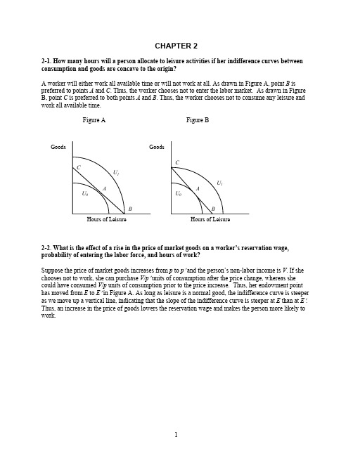
CHAPTER 22-1. How many hours will a person allocate to leisure activities if her indifference curves between consumption and goods are concave to the origin?A worker will either work all available time or will not work at all. As drawn in Figure A, pointB is preferred to points A andC . Thus, the worker chooses not to enter the labor market. As drawn in Figure B, point C is preferred to both points A and B . Thus, the worker chooses not to consume any leisure and work all available time.Figure A Figure B2-2. What is the effect of a rise in the price of market goods on a worker’s reservation wage, probability of entering the labor force, and hours of work?Suppose the price of market goods increases from p to p ′ and the person’s non-labor income is V . If she chooses not to work, she can purchase V/p ′ units of consumption after the price change, whereas she could have consumed V/p units of consumption prior to the price increase. Thus, her endowment point has moved from E to E ′ in Figure A. As long as leisure is a normal good, the indifference curve is steeper as we move up a vertical line, indicating that the slope of the indifference curve is steeper at E than at E ′. Thus, an increase in the price of goods lowers the reservation wage and makes the person more likely to work.Hours of LeisureHours of LeisureGoods GoodsBCA ABCU 1U 1U 0U 0Figure A.To simplify the illustration of the effect on hours of work, assume for simplicity that V = 0. The increase in the price of goods shifts the budget line from FE to GE , moving the worker from P to point R . This shift induces both an income effect and a substitution effect. The price increase in effect lowers the person’s real wage rate, increasing the demand for leisure and leading to fewer hours of work. Thissubstitution effect is illustrated by the move from point P to point Q in Figure B. The price increase also reduces the worker’s wealth, lowering the demand for leisure and leading to more hours of work. This income effect is illustrated by the move from Q to R . As drawn the income effect dominates thesubstitution effect and the price increase lowers the demand for leisure and increases hours of work. It is, of course, possible for the substitution effect to dominate the income effect (not pictured), so that hours of work decreases. Thus, without further restrictions on preferences, an increase in the price of market goods has an ambiguous effect on hours worked.Figure B.GoodsV /p ′V /LeisureHours of Leisure2-3. Sally can work up to 3,120 hours each year (a busy social life and sleep take up the remaining time). She earns a fixed hourly wage of $25. Sally owes a 10 percent payroll tax on the first $40,000 of income. Above $40,000 of income, there is no payroll tax. Sally also faces a progressive income tax rate. There is no income tax on the first $10,000 of income. From $10,000 up to $60,000, the marginal income tax rate is 25 percent. Above $60,000, the marginal income tax rate is 50 percent. Graph Sally’s budget line.Sally’s budget line will have kinks at gross income levels of $10,000, $40,000, and $60,000. As her wage is $25 per hour, these kinks occur after 400 hours, 1,600 hours, and 2,400 hours of work respectively, or, similarly, at 2,720, 1,520, and 720 hours of leisure.•From 0 to 400 hours, Sally’s after-tax wage is $22.50 (90 percent of $25). If she works exactly 400 hours, her after-tax income is $9,000.•From 400 to 1,600 hours, Sally’s after-tax wage is $16.25 (65 percent of $25). If she works exactly 1,600 hours, her after-tax income is $9,000 + $16.25 (1600-400) = $28,500.•From 1,600 to 2,400 hours, Sally’s after-tax wage is $18.75 (75 percent of $25). If she works exactly 2,400 hours, her after-tax income is $28,500 + $18.75 (2400-1600) = $43,500.•From 2,400 to 3,120 hours, Sally’s after-tax wage is $12.50 (50 percent of $25). If she works exactly 3,120 hours, her after-tax income is $43,500 + $12.50 (3120-2400) = $52,500.2-4. Tom earns $15 per hour for up to 40 hours of work each week. He is paid $30 per hour for every hour in excess of 40. Tom faces a 20 percent tax rate and pays $4 per hour in child care expenses for each hour he works. Tom receives $80 in child support payments each week. There are 168 hour in the week. Graph Tom’s weekly budget line.•If Tom does not work, he leisures for 168 hours and consumes $80.•For all hours Tom works up to his first 40, his after-tax and after-child care wage equals (80 percent of $15) – $4 = $8 per hour. Thus, if he works for 40 hours, he will be able to leisure for 128 hours and consume $80 + $8(40) = $400.•For all hours Tom works over 40, his after-tax and after-child care wage equals (80 percent of $30) – $4 = $20. Thus, if he works for 168 hours (128 hours at the overtime wage), he will notleisure at all, but he will consume $80 + $8(40) + $20(128) = $2,960.2-5. What happens to a worker’s desired hours of work if employers pay an overtime premium equal to “time and a half”(that is, 1.5 times the straight-time wage) for any hours worked in excess of 40 hours? What would happen to hours of work if the overtime premium were raised to double the straight-time wage?The availability of overtime pay generates a new (steeper) segment of the budget line originating at the point where the person works 40 hours per week. The figure below illustrates three different possibilities. If the person works 40 hours per week (person B), he or she will be better off by moving to the tangency point labeled X. This person, therefore, will take advantage of the overtime pay and work more hours. If the person is working more than 40 hours per week initially (as is the case for person C), the move from C to X involves both income and substitution effects, and hence we cannot determine which effect dominates. If the person works many fewer than 40 hours per week (person A) he or she will not be affected by the possibility of overtime pay. If the overtime pay were increased to double-pay, it would steepen the line segment originating at 40 hours of work, and perhaps induce some of the persons like A to take advantage of the overtime pay. Person B would continue to work more than 40 hours under a double-time rate, while the double-time rate would have an ambiguous effect on the hours worked of person C.Dollars of Consumption$2,960$400 $80128 168 Hours of LeisureTom’s Weekly Budget Line2-6. A person owns a small farm near a large city and must decide whether to work on that small farm or take a job in the city. Her utility depends on her income per day, Y , and the number of hours allocated to leisure activities, L . Daily income from farm work is:220f f f h h Y −=,where h f is hours of work on the farm; and daily income from the city job is:Y C = 14h C ,where h C is hours of work in the city.To calculate the budget lines associated with each of the opportunities, it is easiest to work through a numerical calculation of what a worker’s earnings would be if he or she allocated 1 hour, 2 hours, 3 hours, etc., to each of the sectors and worked in that sector exclusively. This calculation leads to:Total Earnings Marginal EarningsHours of Work Farm City Farm City1 19 14 19 142 36 28 17 143 51 42 15 14 4 64 56 13 145 75 70 11 146 84 84 9 147 91 98 7 14 8 96 112 5 14Consumption ($)Leisure(a) If she can work on the farm or in the city, but not both, which sector would she choose?The table above suggests the budget line associated with working exclusively in the city is given by CE and on the farm is the parabola FE . As a result, if a worker can only work in either the city or on the farm, a worker with indifference curves like person A is better off working on the farm, while a worker with indifference curves like person B is better off in the city.(b) If she can work both on the farm and in the city, how would she allocate her time?If a worker can allocate her time to both the city and the farm, the worker is then better off allocating the first few hours of work to the farm sector. As the table indicates, the first hour allocated to the farm sector generates $19 worth of income, the second hour generates $17, the third hour generates $15, the fourth hour generates $13, and so on. The worker is thus best off by allocating the first three hours to the farm sector and working any remaining hours she wishes in the city where each additional hour of work generates a constant $14.2-7. Cindy gains utility from consumption C and leisure L . The most leisure she can consume in any given week is 168 hours. Her utility function is U(C,L) = C × L . This functional form implies that Cindy’s marginal rate of substitution is C / L . Cindy receives $630 each week from her great-grandmother – regardless of how much Cindy works. What is Cindy’s reservation wage?The reservation wage is the MRS when not working at all. Thus, w RES = MRS at maximum leisure = C / L = $630 / 168 = $3.75.Leisure2-8. The utility function of a worker is represented by U(C, L) = C ×L, so that the marginal utility of leisure is C and the marginal utility of consumption is L. Suppose this person currently has a weekly income of $600 and chooses to enjoy 70 hours of leisure per week. How many additional dollars of income would it take to entice the worker to work 10 more hours?Initially the person’s utility is U(C,L) = U(600,70) = 600 × 70 = 42,000. She would agree to work 10 more hours (i.e., give up 10 hours of leisure) if the increase in consumption would allow her to achieve at least the same level of utility. Letting Y be her new total income, therefore, Y must solve 60Y = 42,000, which requires Y = $700. Thus, the person’s income would have to rise by $100 to compensate her for the loss of 10 hours of leisure.2-9. You can either take a bus or drive your car to work. A bus pass costs $5 per week, whereas driving your car to work costs $60 weekly (parking, tolls, gas, etc.). You spend half-an-hour less on a one-way trip in your car than on a bus. How would you prefer to travel to work if your wage rate is $10 per hour? Will you change your preferred mode of transportation if your wage rate rises to $20 per hour? Assume you work five days a week and time spent riding on a bus or driving a car does not directly enter your utility.Taking a bus will save you $55 a week, but it will cost you 5 hours of leisure time due to the longer commute. Since the price of leisure is equal to the wage rate, the monetary value of the time lost is $50 when the hourly wage is $10 and $100 when the hourly wage is $20. Therefore, it makes sense for you to take a bus to work if you are paid $10 per hour, but you will switch to driving your car if your wage increases to $20 per hour.2-10. Shelly’s preferences for consumption and leisure can be expressed asU(C,L) = ( C – 200 )× ( L – 80 ).This utility function implies that Shelly’s marginal utility of leisure is C – 200 and her marginal utility of consumption is L – 80. There are 168 hours in the week available to split between work and leisure. Shelly earns $5 per hour after taxes. She also receives $320 worth of welfare benefits each week regardless of how much she works.(a) Graph Shelly’s budget line.If Shelly does not work, she leisures for 168 hours and consumes $320. If she does not leisure at all, she consumes $320 + $5(168) = $1,160.(b) What is Shelly’s marginal rate of substitution when L = 100 and she is on her budget line?If Shelly leisures for 100 hours, she works for 68 hours and consumes $320 + $5(68) = $660. Thus, her MRS when doing this is:23$204608010020066080200==−−=−−==L C MUcMU MRS L .(c) What is Shelly’s reservation wage?The reservation wage is defined as the MRS when working no hours. When working no hours, Shelly leisures for 168 hours and consumes $320. Thus,36.1$8812080168200320≈=−−=RES w .Dollars of Consumption$1,160$320168 Hours of LeisureShelly’s Weekly Budget Line(d) Find Shelly’s optimal amount of consumption and leisure.Her optimal mix of consumption and leisure is found by setting her MRS equal to her wage and solving for hours of leisure given the budget line: C = 320 + 5(168–L )..1365960400580200)168(53205802005=−=−−−−+=−−==L LL L L L C MRSwThus, Shelly will choose to leisure 136 hours, work 32 hours, and consume $320 + $5(32) = $480 each week.2-10. Among single, college-educated women aged 22 – 25, average annual hours worked is 2,160 and the average wage is $22.50. If the average wage increases to $25 per hour, average annual hours worked increases to 2,340. What is the elasticity of labor supply for this group of workers?The elasticity of labor supply is75.09112150.2250.2200.25160,2160,2340,2%%==−−=∆∆=wL S σ.2-11. Mike’s utility for consumption and leisure is U(C,L) = C × L so that his marginal rate ofsubstitution between leisure and consumption is C/L . There are 168 hours in the week and he earns $10 per hour.(a) What is Mike’s optimal amount of consumption and leisure?Mike’s optimal mix of consumption and leisure is found by setting his MRS equal to his wage and solving for hours of leisure given that the budget line is C = 10(168–L ).. 84101680 1010=−== =L LLLCMRS wThus, Mike will choose to leisure 184 hours, work 84 hours, and consume $10(84) = $840 each week. (b) If the government starts a welfare policy that pays B to all non-workers and pays $0 to all workers, at what value of B will Mike opt out of the labor force in order to go on welfare?Given our answer in part (a), we know that if Mike opts to work, his utility will be u work(840,84) =840(84) = 70,560. If he opts out of the labor market, his utility will be u welfare(B,168) = 168B. Mike will not work, therefore, as long as u welfare≥ u work, which requires that B≥ $420.2-12. Explain why a lump sum government transfer can entice some workers to stop working (and entices no one to start working) while the earned income tax credit can entice some people who otherwise would not work to start working (and entices no one to stop working).A lump sum transfer is associated with an income effect but not a substitution effect, because it doesn’t affect the wage rate. Thus, if leisure is a normal good, a lump sum transfer will likely cause workers to work fewer hours (and certainly not cause them to work more hours) while possibly enticing some workers to exit the labor force. On the other hand, the Earned Income Tax Credit raises the effective wage of low-income workers by 20 percent (at least for the poorest workers). Thus, someone who had not been working faces a wage that is 20 percent higher than it otherwise was. This increase may be enough to encourage the person to start working. For example, if a worker’s reservation wage is $6.50 per hour but the only job she can find pays $6.00 per hour, she will not work. Under the earned income tax credit, however, the worker views this same job as paying $7.20 per hour, which exceeds her reservation wage. Furthermore, the EITC cannot encourage a worker to exit the labor force, as the benefits of the EITC are received only by workers.2-13. In 1999, 4,860 TANF recipients were asked how many hours they worked in the previous week. In 2000, 4,392 of these recipients were again subject to the same TANF rules and were again asked their hours of work during the previous week. The remaining 468 individuals were randomly assigned to a “Negative Income Tax” (NIT) experiment which gave out financial incentives for welfare recipients to work and were subject to its rules. Like the other group, they were asked about their hours of work during the previous week. The data from the experiment are contained in the table below.TotalNumber OfRecipients Number ofRecipients Who Worked At Some Time in the SurveyWeek Total Hours Of Work By All Recipients in the Survey Week1999 2000 1999 2000TANF 4,392 1,217 1,568 15,578 20,698NIT 468 131 213 1,6382,535Total 4,860 1,348 1,781 17,21623,233(a) What effect did the NIT experiment have on the employment rate of public assistance recipients? Develop a standard difference-in-differences table to support your answer.EmploymentRate1999 2000 Diff Diff-in-DiffTANF 27.7% 35.7% 8.0%NIT 28.0% 45.5% 17.5% 9.5%The NIT increased the probability of employment by 9.5 percentage points.(b) What effect did the NIT experiment have on the weekly hours worked of public assistance recipients who worked positive hours during the survey week? Develop a standard difference-in-differences table to support your answer.Weekly Hours Worked Per Working Person1999 2000 Diff Diff-in-DiffTANF 12.8 13.2 0.4NIT 12.5 11.9 -0.6 -1.0The NIT decreased weekly hours worked, of those working, by 1 hour.11。

劳动经济学课后题答案

劳经复习资料第一章：1、谈谈你对劳动经济学研究表述的理解:劳动经济学的研究对象:第一：在效用最大化假设下，劳动力资源的投入产出机理。

第二：劳动经济学研究劳动力市场的运行和结果.第三：劳动经济学是对劳动力资源配置的市场经济活动过程中的劳动力需求和供给的行为及其影响因素的分析和研究。

劳动经济学研究方法：第一:实证经济学分析方法:在一定的假设前提下，人们的行为是怎样的。

两个假设前提:稀缺性;理性第二:规范经济学研究方法：用一定的价值观去衡量经济效益的好坏和制度政策的利弊，分析经济行为人的选择该是什么的问题劳动经济学的研究特点：第一：将问题的注意力投向了人们的工作范围第二:研究劳动经济问题的时候，不能脱离商品市场和资本市场来孤立的进行劳动经济的分析和研究。

2、举例说明运用实证经济学或规范经济学研究现实劳动经济或者人力资源管理问题的价值。

规范经济学:从本质上讲，它的根本价值尺度是以互惠原则作为基础的出发点，互惠原则有三点:第一：市场交易活动所涉及的各方均受益，无人受到损失。

例如:企业高薪聘用经验丰富，能力足够强的外籍主管,对企业方来说此人将给企业带来相当大的价值，对个人来说将获取丰厚的回报.第二:市场交易活动中,部分人受益但无人受到损失。

正如上例所说，在企业和个人双方均获得收益时,对于其他那些企业或者市场上的高管应聘者来说，并未因此受到损失。

第三：最为常见的既有受益者又有损失者，但总体上来说，受益者受益的程度或数量超过损失者损失的程度或数量。

例如在很多发达国家的劳动立法反对招聘中的学历歧视，对有的企业带来招聘成本的上升，但是对总体而言提高了社会人力资源配置的效率，利大于弊。

第二章：名词解释：1.派生需求（简答题）：是指对生产要素的需求,意味着它是由对该要素参与生产的产品的需求派生出来的,又称“引致需求”，即对一种生产要素的需求来自对另一种产品的需求。

2.劳动的边际成本:使用一单位量劳动力所耗费的成本,即工资3.劳动的边际收益：增加一单位量的劳动力所增加的收益，即劳动边际产品价值4.使用劳动要素的原则：增加一单位劳动的使用所带来的“边际收益”和“边际成本”必须相等5.竞争性劳动市场：产品和要素市场上供求的双方人数都很多，产品要素之间没有区别，产品和要素的供求双方都具有完全的信息并且可以充分自由的流动6.买方垄断企业：是指企业劳动力市场是垄断者，而在产品市场上是完全竞争者7.劳动的边际产品价值（就是劳动的边际收益)8.替代效应：劳动使用量从LA降低到LB,资本使用量从KA上升到KB，即企业用资本代替了劳动。

《劳动经济学》作者Borjas 习题答案

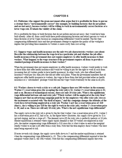
CHAPTER 66-1. Politicians who support the green movement often argue that it is profitable for firms to pursue a strategy that is “environmentally correct” (for example, by building factories that do not pollute and are not noisy), because workers will be willing to work in environmentally correct factories at a lower wage rate. Evaluate the validity of this claim.If it is profitable for firms to build factories that do not pollute and are not noisy, they would have been built already. After all, firms could build these profit-maximizing factories and attract persons to work at these factories at lower wages because no compensating differential would be needed. The fact that compensating differentials exist and that governments attempt to regulate the quality of the workplace implies that providing these amenities to workers is more costly than cost-saving.6-2. Suppose wages and health insurance are the only two job characteristics workers care about. Describe the relationship between the wage level in a particular job and whether the job offers health insurance if the government does not require employers to offer health insurance to their workers. What happens to the wage structure if the government requires all firms to provide a standard package of health insurance to their workers?When the government does not require employers to offer health insurance, workers would prefer to work in those firms that offer health insurance and would be willing to pay for the right to work in such firms (assuming that all workers prefer to have health insurance). In other words, jobs that offered health insurance would pay less than jobs that did not offer such plans. When the government mandates that all employers offer health insurance to workers, the wage in those firms that had provided either no health insurance or a “substandard” package would fall and the wage would eventually be the same in all jobs. 6-3. Workers choose to work a risky or a safe job. Suppose there are 100 workers in the economy. Worker 1’s reservation price (for accepting the risky job) is $1; worker 2’s reservation price is $2, and so on. Because of technological reasons, there are only 10 risky jobs. What is the equilibrium wage differential between safe and risky jobs? Which workers will be employed at the risky firm? Suppose now that an advertising campaign paid for by the employers who offer risky jobs stresses the excitement associated with “the thrill of injury,” and this campaign changes the attitudes of the work force toward being employed in a risky job. Worker 1 now has a reservation price of -$10 (that is, she is willing to pay $10 for the right to work in the risky job); worker 2’s reservation price is -$9, and so on. There are still only 10 risky jobs. What is the new equilibrium wage differential? The supply curve to the risky job is given by the fact that worker 1 has a reservation price of $1, worker 2 has a reservation price of $2, and so on. As the figure below illustrates, this supply curve (given by S) is upward sloping, and has a slope of 1. The demand curve (D) for risky jobs is perfectly inelastic at 10 jobs. Market equilibrium is attained where supply equals demand so that 10 workers are employed in risky jobs; the market compensating wage differential is $10 since this is what it takes to entice the marginal (tenth) worker to accept a job offer from a risky firm. Note that the firm employs those workers who least mind being exposed to risk.If tastes towards risk change, the supply curve shifts down to S′ and the market equilibrium is attained when the compensating wage differential is -$1. This is the compensating differential required to hire the marginal worker (that is, the 10th worker). Note that this compensating differential implies that eventhough most workers (from worker 12 onwards) dislike risk, the market determines that risky jobs will pay less than safe jobs.6-4. Suppose all workers have the same preferences represented byU w x ,=−2where w is the wage and x is the proportion of the firm’s air that is composed of toxic pollutants. There are only two types of jobs in the economy, a clean job (x = 0) and a dirty job (x = 1). Let w 0 be the wage paid by the clean job and w 1 be the wage paid by the polluted job. If the clean job pays $16 per hour, what is the wage in dirty jobs? What is the compensating wage differential?If all persons have the same preferences regarding working in a job with polluted air, market equilibrium requires that the utility offered by the clean job be the same as the utility offered by the dirty job, otherwise all workers would move to the job that offers the higher utility. This implies that:)1(2)0(210−=−w w => .2161−=wSolving for w 1 implies that w 1 = $36. The compensating wage differential, therefore, is $20.C om pensatin gDm ent6-5. Suppose a drop in the compensating wage differential between risky jobs and safe jobs has been observed. Two explanations have been put forward:• Engineering advances have made it less costly to create a safe working environment.• The phenomenal success of a new action serial “Die On The Job!” has imbued millions ofviewers with a romantic perception of work-related risks.Using supply and demand diagrams show how each of the two developments can explain the drop in the compensating wage differential. Can information on the number of workers employed in the risky occupation help determine which explanation is the right one?The engineering advances make it cheaper for firms to offer safe jobs, and hence reduce the gain from switching from a safe environment to a risky one. This will shift the demand curve for risky jobs in and reduce the compensating wage differential (Figure 1). Note that the equilibrium number of workers in risky jobs goes down.The glamorization of job-related risks may make people more willing to take these risks. This shiftssupply to the right and reduces the compensating differential (Figure 2). Note that the equilibrium number of workers in risky jobs goes up.Thus, information on whether employment in the risky sector increased or decreased can help discern between the two competing explanations.Figure 1. Labor Market for Risky JobsCompensatingDifferentialE new E old Number of Workers in Risky Jobs(w 1 – w 0 )old (w 1 – w 0 )Figure 2. Labor Market for Risky Jobs6-6. Consider a competitive economy that has four different jobs that vary by their wage and risk level. The table below describes each of the four jobs.Job Risk ( r ) Wage ( w )A 1/5 $3B 1/4 $12C 1/3 $23D 1/2 $25All workers are equally productive, but workers vary in their preferences. Consider a worker who values his wage and the risk level according to the following utility function:u w r w r (,)=+12.Where does the worker choose to work? Suppose the government regulated the workplace and required all jobs to have a risk factor of 1/5 (that is, all jobs become A jobs). What wage would the worker now need to earn in the A job to be equally happy following the regulation?Calculate the utility level for each job by using the wage and the risk level: U(A) = 28, U(B) = 28, U(C) = 32, and U(D) = 29. Therefore, the worker chooses a type C job and receives 32 units of happiness. If she is forced to work a type A job, the worker needs to receive a wage of $7 in order to maintain her 32 unitsof happiness as 7 + 25 = 32.CompensatingDifferential E old E new Number of Workers in Risky Jobs(w 1 – w 0 )old (w 1 – w 0 )6-7. Consider Table 6-1 and compare the fatality rate of workers in the agricultural, mining, construction, and manufacturing industries?(a) What would the distribution of wages look like across these four industries given the compensating differential they might have to pay to compensate workers for risk?Mining would pay the highest compensating differential, followed by agriculture, then construction, and finally manufacturing.(b) Now look at the median weekly earnings by industry as reported in Table 629 of the 2002 U.S. Statistical Abstract. Does the actual distribution of wages reinforce your answer to part (a)? If not, what else might enter the determination of median weekly earnings?Median weekly earnings by industry are:$795Mining$371Agriculture$609Construction$613ManufacturingThus, the distribution of wages does not perfectly reflect the compensating differential story, though mining is the best paid and the most dangerous. It is also the unhealthiest, which workers would supposedly take into account as well. Many other factors, however, probably explain the wage structure just as much if not more than compensating differentials, including preferences (family farmers), unions (manufacturing), required skills, and the length of the average work week.6-8. The EPA wants to investigate the value workers place on being able to work in “clean” mines over “dirty” mines. The EPA conducts a study and finds the average wage in clean mines to be $42,250 and the average wage in dirty mines to be $47,250.(a) According to the EPA, how much does the average worker value working in a clean mine?The average value is $47,250 - $42,250 = $5,000.(b) Suppose the EPA could mandate that all dirty mines become clean mines and that all workers who were in a dirty mine must therefore accept a $5,000 pay decrease. Are these workers helped by the intervention, hurt by the intervention, or indifferent to the intervention?All except the marginal worker are hurt by the intervention. The workers who sort themselves into the dirty jobs are those workers that do not mind dirt, and therefore do not value working in a clean job at $5,000. (Similarly, if all of the workers in the clean jobs were forced to accept dirty jobs for $5,000 more, all of them except the marginal worker would be hurt as they all value working in a clean job at more than $5,000.)6-9. There are two types of farming tractors on the market, the FT250 and the FT500. The only difference between the two is that the FT250 is more prone to accidents than the FT500. Over their lifetime, one in ten FT250s is expected to result in an accident, as compared to one in twenty-five FT500s. Further, one in one-thousand FT250s is expected to result in a fatal accident, as compared to only one in five-thousand FT500s. The FT250 sells for $125,000 while the FT500 sells for $137,000. At these prices, 2,000 of each model are purchased each year. What is the statistical value farmers place on avoiding a tractor accident? What is the statistical value of a life of a farmer? The FT500 is associated with an extra cost of $12,000, but its accident rate is only 0.04 compared to the 0.10 accident rate of the FT250. Also, each farmer that buys the FT250 is willing to accept the additional risk in order to save $12,000. Thus, these workers are willing to receive $24 million ($12,000 x 2,000) in exchange for 200 – 80 = 120 accidents. Thus, the value placed on each accident is $200,000. Likewise, the 2,000 farmers who buy the FT250 are willing to receive $24 million in exchange for 2 – .4 = 1.6 fatal accidents. Thus, the value placed on each life is $15 million.6-10. Consider the labor market for public school teachers. Teachers have preferences over their job characteristics and amenities.(a) One would reasonably expect that high-crime school districts pay higher wages than low-crime school districts. But the data consistently reveal that high-crime school districts pay lower wages than low-crime school districts. Why?The likely reason for this is not that teachers do not care about crime – they almost certainly do – but rather that school funding is determined in large part by local property taxes. If high crime schools are located in low income cities, there is nothing (or at least very little) the local school board can do to raise more money to pay the compensating differential.(b) Does your discussion suggest anything about the relation between teacher salaries and school quality?In the end, because high crime schools cannot offer the necessary compensating differential, they will not be able to attract the highest quality workers. Therefore, one would expect that the worst schools (with the worst teachers) are located in the poorest communities with the most crime. This is the typical story of proponents of replacing the property tax scheme to fund public education with a federal program.6–11. Many employers willingly offer their employees certain benefits such as health insurance, a retirement plan, gym memberships, or even an on-site subsidized cafeteria. Why?Offering job benefits is identical to offering a job with bad characteristics such as risk. When offering a risky job, for example, the employer must buy-off the risk from the worker. The employer chooses to do this because it is profitable, i.e., because the cost of buying-off the risk is less costly than transforming the job into a safe one. The same (but opposite) argument holds for job benefits. By offering a job with benefits, the employer can pay the worker less as the worker values the benefits. The employer will find it profitable to continue to offer benefits as long as the employer can save more in reducing the wage than it costs to provide the benefits.One reason health insurance benefits are fairly popular is that firms can usually negotiate lower prices and better packages of care than individuals can do by themselves. Also, firms can deduct the cost of their benefits from their net revenue, whereas individuals cannot deduct the full amount of their healthcare expenses.。

劳动经济学课后答案

对一种生产要素的需求来自（派生自）对另一种产品的需求。

其中该生产要素对这一最终产品会作贡献，如对轮胎的需求派生自对汽车运输的需求。

1.短期：在短期内可变的生产要素只有劳动力，技术和资本都是不变生产要素。

2.长期：在长期内，劳动力和技术是可变生产要素，只有资本是不变生产要素。

3.卖方垄断企业：指企业在产品市场上市垄断者，但在劳动市场上市完全竞争。

4.买方垄断企业：是指企业劳动力市场是垄断者，而在产品市场上是完全竞争者。

5.替代效应:劳动使用量从LA降低到LB，资本使用量从KA上升到KB，即企业用资本代替了劳动。

7.互补性生产要素：当生产要素A的价格下降，数量增加时，对生产要素B的需求上升，则称生产要素A与生产要素B是互补。

8.替代性生产要素：当生产要素A的价格下降，数量增加时，生产要素B的数量下降，则生产要素A是生产要素B的替代性生产要素。

9.劳动需求的工资弹性：a)劳动需求的工资弹性是指当工资率变化一个百分率所引起的劳动需求变化的百分率的比值。

b)公式：ed ＝－(△L/L)/(△W/W)＝－(△L/△W)/(W/L)1.ed为劳动需求的工资弹性，△L和△W分别是劳动需求数量L和工资率W的变动量。

10、劳动的边际产品价值：VMP=MP•P，指的是增加额外一单位劳动要素的投入所带来的收益。

（三）1.劳动力：是人的劳动能力，即人在劳动过程中所运用的体力和智力的总和。

在现代劳动经济学体系中，劳动力又特指在一定年龄范围内，具有劳动能力和劳动要求。

《劳动经济学》(作者Borjas)第七章习题答案

CHAPTER 77-1. Debbie is about to decide which career path to pursue. She has narrowed her options to two alternatives. She can either become a marine biologist or a concert pianist. Debbie lives two periods. In the first, she gets an education. In the second, she works in the labor market. If Debbie becomes a marine biologist, she will spend $15,000 on education in the first period and earn $472,000 in the second period. If she becomes a concert pianist, she will spend $40,000 on education in the first period and then earn $500,000 in the second period.(a) Suppose Debbie can lend and borrow money at a 5 percent annual rate. Which career will she pursue? What if she can lend and borrow money at a 15 percent rate of interest? Will she choose a different option? Why?Debbie will compare the present value of income for each career choice and choose the career with the largest present value. If the discount rate is 5 percent,PV Biologist = – $15,000 + $472,000/(1.05) = $434,523.81andPV Pianist = – $40,000 + $500,000/(1.05) = $436,190.48.Therefore, she will become a pianist. If the rate of interest is 15 percent, however, the present value calculations becomePV Biologist = – $15,000 + $472,000/(1.15) = $395,434.78andPV Pianist = – $40,000 + $500,000/(1.15) = $394,782.61.In this case, Debbie becomes a biologist. As the interest rate increases, the worker discounts future earnings more, lowering the returns from investing in education.(b) Suppose musical conservatories raise their tuition so that it now costs Debbie $60,000 to become a concert pianist. What career will Debbie pursue if the discount rate is 5 percent?Debbie will compare the present value of being a biologist from part (a) with the present value of becoming a pianist. The relevant present values are:PV Biologist = – $15,000 + $472,000/(1.05) = $434,523.81andPV Pianist = – $60,000 + $500,000/(1.05) = $416,190.48.Debbie will, therefore, become a biologist.7-2. Peter lives for three periods. He is currently considering three alternative education-work options. He can start working immediately, earning $100,000 in period 1, $110,000 in period 2 (as his work experience leads to higher productivity), and $90,000 in period 3 (as his skills become obsolete and physical abilities deteriorate). Alternatively, he can spend $50,000 to attend college in period 1 and then earn $180,000 in periods 2 and 3. Finally, he can receive a doctorate degree in period 2 after completing his college education in period 1. This last option will cost him nothing when he is attending graduate school in the second period as his expenses on tuition and books will be covered by a research assistantship. After receiving his doctorate, he will become a professor in a business school and earn $400,000 in period 3. Peter’s discount rate is 20 percent per period. What education path maximizes Peter’s net present value of his lifetime earnings?The present discounted values of Peter’s earnings associated with each of the alternatives are167,254$2.1000,902.1000,110000,1002=++=HS PV , 000,225$2.1000,1802.1000,180000,502=++−=COL PV , and 778,227$2.1000,4002.10000,502=++−=PhD PV .Thus, the best option for Peter is to start working upon completely high school.7-3. Jane has three years of college, Pam has two, and Mary has one. Jane earns $21 per hour, Pam earns $19, and Mary earns $16. The difference in educational attainment is due completely to different discount rates. How much can the available information reveal about each woman’s discount rate?The returns to increasing one’s education from one to two years of college and then from two to three years of college are%75.1816$16$19$21=−=to r and %53.1019$19$21$32=−=to r .Having observed their educational choices, we know that Mary’s discount rate is greater than 18.75 percent, Pam’s is between 10.53 percent and 18.75 percent, and Jane’s is less than 10.53 percent.7-4. Suppose the skills acquired in school depreciate over time, perhaps because technologicalchange makes the things learned in school obsolete. What happens to a worker’s optimal amount of schooling if the rate of depreciation increases?If the rate of depreciation is very high, the payoff to educational investments declines. As a result, a worker’s optimal amount of schooling will also fall as the benefits of education erode rapidly.7-5. Suppose workers differ in their ability, but have the same discount rate. Is it possible for the more able workers to choose less schooling?This result is possible as long as more able workers have lower marginal-rate-of-discount curves. For example, if an 18-year-old basketball player can earn $3 million per year by entering the NBA after high school whereas he would earn $3.25 million per year by entering the NBA after college, the opportunity cost of college ($3 million per year) may be so great that the player opts to skip college. (A similar story might explain why Bill Gates dropped out of Harvard.)7-6. Suppose Carl’s wage-schooling locus is given byYears of Schooling Earnings6 $10,0007 $12,8008 $16,0009 $18,50010 $20,35011 $22,00012 $23,10013 $23,90014 $24,000(a) Derive the marginal rate of return schedule. When will Carl quit school if his discount rate is 4 percent? What if the discount rate is 12 percent?The marginal rate of return is given by the percentage increase in earnings if the worker goes to school one additional year.Schooling Earnings MRR6 $10,00028.07 $12,80025.08 $16,0009 $18,50015.610 $20,350 10.011 $22,000 8.112 $23,100 5.013 $23,900 3.514 $24,000 0.4Carl will quit school when the marginal rate of return to schooling falls below his discount rate. If his discount rate is 4 percent, therefore, he will quit after 12 years of schooling; if his discount rate is 12 percent, he will quit after 9 years of schooling.(b) Suppose the government imposes an income tax of 20 percent on both labor earnings and interest income. What is the effect of this income tax on Carl’s educational attainment?This is a tricky problem. If Carl is making his educational decision by comparing the marginal rate of return to schooling to some rate of discount that does not depend on the government’s tax policies, then it turns out that Carl’s optimal schooling level is unchanged. It is easy to verify that if the governmentimposes a 20 percent tax rate on labor earnings in the second column of the table above, the marginal rate of return to schooling (column 3) remains unchanged. If, however, Carl’s rate of discount is affected by the government’s tax policies (for example, Carl’s rate of discount might be affected by the rate of interest banks pay), then Carl’s educational decision will be affected. For example, if Carl’s rate of discount falls by 20 percent then the amount of schooling acquired goes up because the marginal rate of return schedule in column 3 of the table has changed.7-7. In the typical signaling model, it is assumed that the costs of acquiring an education are higher for low-ability than for high-ability workers. Suppose the government subsidizes low-ability workers for the higher costs they incur in obtaining an education. What happens to the signaling value of education? Can there be a perfectly separating equilibrium in this labor market?If the government subsidizes schooling so that the cost of schooling is the same for all workers, then the signaling value of schooling is lost. There cannot be a perfectly separating equilibrium because all workers would have the same incentive to obtain the same amount of schooling.7-8. Suppose there are two types of persons: high-ability and low-ability. A particular diploma costs a high-ability person $8,000 and costs a low-ability person $20,000. Firms wish to use education as a screening device where they intend to pay $25,000 to workers without a diploma and $K to those with a diploma. In what range must K be to make this an effective screening device?In order for a low-ability worker to not pursue education, it must be that $25,000 ≥K – $20,000 which requires K≤ $45,000. Similarly, in order for a high-ability worker to pursue education, it must be that K – $8,000 ≥ $25,000 which requires K≥ $33,000. Thus, in order to use education as a signaling device, it must be that educated workers are paid between $33,000 and $45,000.7-9. It has been argued that the minimum wage prevents workers from investing in on-the-job training and discourages employers from providing specific training to low-income workers. Why would the minimum wage have an adverse effect on human capital accumulation for low-income workers?First, when the minimum wage is high, the marginal return to on-the-job investment falls (assuming one can always find a job), and therefore the lowest skill workers may no longer find it useful to engage in on-the-job training.Second, a firm that offers general or specific training in the first period pays the worker a wage below his or her marginal product while the investment is taking place and above his or her marginal product in the post-investment period. If the minimum wage prevents the investment-period wage from falling sufficiently, however, firms may not be able to offer the training.7-10. Jill is planning the timing of her on-the-job training investments over the life cycle. What happens to Jill’s OJT investments at every age if(a) the market-determined rental rate to an efficiency unit falls?The marginal revenue of investing in OJT declines so that Jill will invest less at each age.(b) Jill’s discount rate increases?If Jill’s discount rate increases she becomes more “present oriented”, reducing the future benefits associated with OJT. Thus her OJT investments fall.(c) the government passes legislation delaying the retirement age until age 70.The marginal revenue of investing in OJT increases because the payoff period to the investment is longer. Thus, she undertakes more OJT in this case.(d) technological progress is such that much of the OJT acquired at any given age becomes obsolete within the next 10 years.The marginal revenue to investing in OJT declines and the amount of OJT acquired falls.7-11. In 2000, there were about 9 million students in four-year college institutions in the United States. Believing that education is the key to the future, a presidential candidate proposes that the federal government pay the first $3,000 of college expenses each year for everyone attending a four-year college. It is expected that this proposal will encourage 3 million more people to enroll in a four-year college each year, but that the graduation rate will fall from 80 percent to 75 percent. What is the yearly projected cost of the program? What is the average cost of the plan per new student attending a four-year college? What is the average cost of each new four-year college graduate?Under the old plan, 9 million students attended a four-year college each year, with 80 percent (7.2 million) eventually graduating. Under the new plan, 12 million students will attend a four-year college each year, with 75 percent (9 million) eventually graduating. The annual cost of the program, therefore, is 12 million × $3,000 = $36 billion. The average cost of the plan per new college student is $36b / 3m = $12,000. The average cost of each new graduate is $36b / 1.8m = $20,000.7-12. In 1970, men aged 18 to 25 were subject to the military draft to serve in the Vietnam War. A man could qualify for a student deferment, however, if he was enrolled in college and made satisfactory progress on obtaining a degree. By 1975, the draft was no longer in existence. The draft did not pertain to women. Using the data in Table 255 of the 2002 edition of the U.S. Statistical Abstract, use women as the control group to estimate (using the difference-in-differences methodology) the effect abolishing the draft had on male college enrollment.The difference-in-differences table isCollege Enrollment (percentage)Diff-in-diff1970 1975 DiffMen 55.2 52.6 -2.6 -3.1Women 48.5 49.0 0.5Thus, abolishing the draft is estimated to lower the college enrollment rate of men by 3.1 percentage points.。

1、下载文档前请自行甄别文档内容的完整性，平台不提供额外的编辑、内容补充、找答案等附加服务。
2、"仅部分预览"的文档,不可在线预览部分如存在完整性等问题,可反馈申请退款(可完整预览的文档不适用该条件!)。
3、如文档侵犯您的权益，请联系客服反馈,我们会尽快为您处理(人工客服工作时间：9:00-18:30)。

劳动经济学》 作者borjas 习题答案

劳动经济学（Borjas

《劳动经济学》(作者Borjas)第十三章习题答案

劳动经济学鲍哈斯第七版第三章答案

现代劳动经济学课后【伊兰伯格】课后习题答案

劳动经济学课后习题参考答案 (1)

《劳动经济学》作者Borjas习题答案

《劳动经济学》(作者Borjas)第十一章习题答案

《劳动经济学》（作者Borjas）第四章习题答案

劳动经济学课后答案

劳动经济学(作者Borjas)第十章习题答案

《劳动经济学》(作者Borjas)第九章习题答案

《劳动经济学》(作者Borjas)第五章习题答案

《劳动经济学》(作者Borjas)第十二章习题答案

劳动经济学鲍哈斯7e答案

《劳动经济学》(作者Borjas)第四章习题答案

劳动经济学》 作者borjas 习题答案

劳动经济学课后题答案

《劳动经济学》 作者Borjas 习题答案

劳动经济学课后答案

《劳动经济学》(作者Borjas)第七章习题答案

劳动经济学》作者borjas 习题答案

劳动经济学》作者borjas 习题答案

《劳动经济学》作者Borjas 习题答案