现代信号处理论文_AR模型的功率谱估计BURG算法的分析与仿真
AR模型谱估计方法研究及其应用

AR模型谱估计方法研究及其应用摘要数字信号处理(DSP)重要的应用领域之一,是建立在周期信号和随机信号基础上的功率谱估计。
在实际应用中往往不能获得具体信号的表达式,需要根据有限的数据样本来获得较好的谱估计效果,因而谱估计被广泛的应用于各种信号处理中[1]。
本论文研究了功率谱估计的几种常用的方法,包括经典谱估计和现代谱估计的各种方法,且对每种方法的估计质量做了数学推导,并给出仿真程序及仿真图。
经典法主要包括周期图法、自相关法,但这两种方法都存在缺陷,即认为观测数据之外的数据都为零,所以对经典法中的周期图法进行了加窗、平均等修正,因此提出了周期图法的改进方法;现代谱估计的方法分类比较多,AR模型法,MA 模型法和ARMA模型法是现代功率谱估计中最主要的参数模型,本论文着重讨论了AR模型参数法[2]。
同时论文将通过对经典谱估计和现代谱估计的实现方法及仿真图的比较,得出经典功率谱估计方法的方差性较差,分辨率较低,而现代谱估计的目标正是在于努力改善谱估计的分辨率,因此能得到较好的谱估计效果,为此应用更为广泛[3]。
关键字:数字信号处理,功率谱估计,周期图法,自相关法,AR模型法ABSTRACTDigital signal processing (DSP) important application of one of the field. Actually, we can’t get the expression of a specific signal, so we need to estimate the power spectral of a signal according to some sample data sequences.So spectrum estimation which is widely used in various signal processing.In this thesis, some common methods of Power Spectral Estimation, such as classical spectral estimation and modern spectral estimation, are studied. The quality of each estimation method is derived, simulation program and simulation figure is given. Classical methods of Power Spectral Estimation mainly include the Periodogram and the BT method. But both of them have a common drawback: the data sequences, beyond the area of the observed sequences, are all presumed to zero. So the Windows and the average method are introduced to improve the quality of the Periodogram. Therefore the improvement of The Periodogram estimation method is proposed. The classification of modern spectral estimation methods are more , AR,MA, and ARMA is the most important parameters of modern spectral estimation. This thesis will focus on discussion of AR model parameters method. At the same time , It can be seen from the comparison and realization of classical spectral estimation and modern spectral estimation, classical power spectrum estimation variance is poor, low resolution .The goal of modern spectral estimation is working to improve the resolution of spectral estimation, better results of the estimation of the power spectrum can be obtained, so it is applied more widely.Keywords: digital signal processing, Power Spectrum Estimation, The Periodogram, the BT methods,AR model目录摘要 (I)1 绪论 (1)1.1功率谱简介 (1)1.2经典谱估计 (2)1.3现代谱估计 (3)1.4功率谱估计应用及用途 (4)2 谱估计简介 (5)2.1随机信号简介 (5)2.2平稳随机信号 (7)2.3估计质量的评价标准 (10)3 现代谱估计 (12)3.1平稳随机信号的参数模型 (12)3.2 AR模型的正则方程与参数计算 (13)3.3 MA模型谱估计 (16)3.4 ARMA模型谱估计 (17)3.5 AR模型功率谱估计实验 (19)3.5.1、实验内容 (19)3.5.2、实验分析 (20)3.5.3、实验结果及分析 (20)3.5.4、实验思考 (24)3.5.5、实验源代码 (25)3.6 AR模型的应用 (30)3.7 小结 (36)4论文总结 (36)参考文献 (38)1 绪论1.1功率谱简介1.功率谱估计技术渊源流长,在过去的几十年获得了飞速的发展。
AR模型谱估计方法研究及其应用

的功率谱密度。
Kalman滤波器的优点是能够实时处理数据,并且能够自适应
03
地调整估计精度。
最小二乘法
最小二乘法是一种常用的参数估计方法,它通 过最小化预测值与实际值之间的残差平方和来 估计模型参数。
在谱估计中,最小二乘法可以用于估计信号的 功率谱密度。
最小二乘法的优点是简单易用,但是它的估计 精度较低,可能会出现偏差。
VS
AR模型可以提取信号中的特征信息 ,从而实现信号的有效分类和识别 ,在语音识别、图像识别等领域有 着广泛的应用前景。
AR模型在信号检测中的应用
利用AR模型对信号进行检测,可以快速准确地检测出信号的 存在和变化情况,及时发现信号中的异常情况。
AR模型可以有效地提取信号中的突变信息,从而实现信号的 有效检测,在雷达、声呐、无线通信等领域有着广泛的应用 。
AR模型的优势
与其他频谱估计方法相比,AR模型具 有多个优点。首先,它可以更加准确 地估计信号的频谱特性,特别是当信 号的噪声水平较高时。其次,它可以 更加灵活地适应不同的信号和系统特 性,从而适用于更广泛的领域。此外 ,AR模型还具有计算复杂度低、易于 实现等优点。
研究内容与方法
研究内容
本文主要研究了AR模型谱估计方法的关键技术,包括 模型的建立、参数估计、性能分析和优化等。在此基 础上,本文还探讨了AR模型在信号处理中的应用,以 及其未来发展趋势和应用前景。
AR模型的参数估计可以采用多种方法,如 最小二乘法、卡尔曼滤波器等。
AR模型的一个重要应用是谱估计, 它可以用于估计信号的频谱特性。
kalman滤波器
01
Kalman滤波器是一种递归滤波器,它通过使用状态空间方法 来估计动态系统的状态变量。
现代信号处理论文(1)
AR 模型的功率谱估计BURG 算法的分析与仿真钱平(信号与信息处理 S101904010)一.引言现代谱估计法主要以随机过程的参数模型为基础,也可以称其为参数模型方法或简称模型方法。
现代谱估计技术的研究和应用主要起始于20世纪60年代,在分辨率的可靠性和滤波性能方面有较大进步。
目前,现代谱估计研究侧重于一维谱分析,其他如多维谱估计、多通道谱估计、高阶谱估计等的研究正在兴起,特别是双谱和三谱估计的研究受到重视,人们希望这些新方法能在提取信息、估计相位和描述非线性等方面获得更多的应用。
现代谱估计从方法上大致可分为参数模型谱估计和非参数模型谱估计两种。
基于参数建摸的功率谱估计是现代功率谱估计的重要内容,其目的就是为了改善功率谱估计的频率分辨率,它主要包括AR 模型、MA 模型、ARMA 模型,其中基于AR 模型的功率谱估计是现代功率谱估计中最常用的一种方法,这是因为AR 模型参数的精确估计可以通过解一组线性方程求得,而对于MA 和ARMA 模型功率谱估计来说,其参数的精确估计需要解一组高阶的非线性方程。
在利用AR 模型进行功率谱估计时,必须计算出AR 模型的参数和激励白噪声序列的方差。
这些参数的提取算法主要包括自相关法、Burg 算法、协方差法、 改进的协方差法,以及最大似然估计法。
本章主要针对采用AR 模型的两种方法:Levinson-Durbin 递推算法、Burg 递推算法。
实际中,数字信号的功率谱只能用所得的有限次记录的有限长数据来予以估计,这就产生了功率谱估计这一研究领域。
功率谱的估计大致可分为经典功率谱估计和现代功率谱估计,针对经典谱估计的分辨率低和方差性能不好等问题提出了现代谱估计,AR 模型谱估计就是现代谱估计常用的方法之一。
信号的频谱分析是研究信号特性的重要手段之一,通常是求其功率谱来进行频谱分析。
功率谱反映了随机信号各频率成份功率能量的分布情况,可以揭示信号中隐含的周期性及靠得很近的谱峰等有用信息,在许多领域都发挥了重要作用。
报告2AR过程的线性建模与功率谱估计

实验报告2——AR过程的线性建模与功率谱估计一、实验目的1.理解AR过程的产生机理,复习实验1估计自相关序列的方法。
2.利用估计出的自相关序列来求解信号的功率谱,即用周期图法来估计功率谱。
3.分别采用自相关法(Yule-Walker法),协方差法,Burg法,修正协方差法来估计功率谱,并与周期图法进行比较,分析性能孰优孰劣。
4.学习matlab在数字信号处理中的应用。
二、实验过程和分析AR过程的线性建模与功率谱估计。
考虑AR过程:=-+-+-+-+()(1)(1)(2)(2)(3)(3)(4)(4)(0)()x n a x n a x n a x n a x n b v n v n是单位方差白噪声。
()(a) 取b(0)=1, a(1)=2.7607, a(2)=-3.8106, a(3)=2.6535, a(4)=-0.9238,产生x(n)的N=256个样点。
用randn(1,N)产生单位方差高斯白噪声v(n),用v(n)激励滤波器产生AR(4)过程,即用x=filter(b,a,v)产生x(n),b是滤波器分子系数,这里为b(0)=1,a是滤波器分母系数,a=[1 -2.7607 3.8106 -2.6535 0.9238]。
(b) 计算其自相关序列的估计ˆ()r k,并与真实的自相关序列值相比较。
x结论:真实自相关序列与估计出的序列对比如上图所示,两者在100点之前的形状相似,幅度有一定差异,而且估计出的自相关序列有较大的波动,这是因为估计的点数较少,使得估计精度不够,另外,估计自相关序列的下标越大,用来估计的点数就越少,因而后面的估计值是很不精确的。
因为假设n>= 500 处的数据为0,所有估计自相关不精确,误差较大。
(c) 将ˆ()x rk 的DTFT 作为x (n )的功率谱估计,即: 1211ˆˆ()()|()|N j jk j xx k N P e rk e X e Nωωω--=-+==∑。
基于BURG算法的谱估计研究和MATLAB实现毕业论文
毕业设计(论文)题目:基于BURG算法的谱估计研究及其MATLAB实现目录一、毕业设计(论文)开题报告二、毕业设计(论文)外文资料翻译及原文三、学生“毕业论文(论文)计划、进度、检查及落实表”四、实习鉴定表XX大学XX学院毕业设计(论文)开题报告题目:基于BURG算法的谱估计研究及其MATLAB实现机电系电子信息工程专业学号:学生:指导教师:(职称:讲师)(职称:)XXXX年XX月X日英文原文Parametric spectral estimation on a single FPGAABSTRACTParametric, model based, spectral estimation techniques can offer increased frequency resolution over conventional short-term fast Fourier transform methods, overcoming limitations caused by the windowing of sampled, time domain, input data. However, parametric techniques are significantly more computationally demanding than the Fourier based methods and require a wider range of arithmetic functionality; for example, operations such as division and square-root are often necessary. These arithmetic processes exhibit communication bottleneck and their hardware implementation can be inefficient when used in conjunction with multipliers. A programmable, bit-serial, multiplier/divider, which overcomes the bottleneck problems by using a data interleaving scheme, is introduced in this paper. This interleaved processor is used to show how the parametric Modified Covariance spectral estimator can be efficiently routed on a field programmable gate array for real-time applications.1. INTRODUCTIONDue to its ease of hardware and software implementation the shortterm fast Fourier transform(STFFT)is widely used for spectral estimation and is known as the conventional method. However, the technique has drawbacks in terms of spectral resolution and accuracy caused by the finite length of the input data sequence used. Windowing of input data causes spectral broadening and Gibb’s phenomenon of spectral leakage can mask the weaker frequency components of the true power spectral density(PSD)[1]. These unwanted effects can be reduced by using longer data sequence lengths, so that the transformed signal becomes a better representation of the infinite data sequence, but in real life this usually is not feasible as the characteristics of the input data may change with time. Over short periods of time the data signals can often be assumed to exhibit wide-sense stationarity, where the signal characteristics are assumed approximately constant but the spectral resolution is therefore limited. In attempts to improve the PSD estimation, windowing functions, Bartlett or Hanning for example, can be used to reduce side-lobe levels but these lower spectral resolution by broadening the main lobe of the PSD[2].Model based, parametric spectral estimation techniques can alternatively be used, where the unrealistic assumption that data is zero outside the window of interest is dropped[1]. Either knowledge of the underlying process or reasonableassumptions about the nature of the unobserved data are used to improve frequencyresolution over the conventional approaches. The computational burden of suchprocessors is however much higher than the STFFT and arithmetic functions such asdivision and square-root often become necessary. In the division and square-rootnon-restoring algorithms there is an inherent dependency that the result bits mustbe computed in a most significant bit(MSB)first manner, with the computation of abit directly dependent upon the result of the previous one[3]. This interdependencymakes it difficult to efficiently realize such arithmetic functions in hardware,and implementations are usually much slower than other basic functions such asmultiplication, addition and subtraction. Communication bottlenecks can thereforeeasily occur in systolic arrays where different types of processors are interconnected.The difficulties with hardware implementation of parametric spectral estimatorshave led to a preference of software implementation on homogeneous DSP networks[4].However, high levels of processing capacity have not been fully reflected in systemthroughput since the increased communication incurred as a result of parallelismis constrained by communication bus performance. This restricts the range ofproblems that can be computed in realtime and the software approach may sometimesbe inadequate for real-time spectral estimation.In this paper, hardware implementation of a parametric spectral estimator isaddressed. A bit-serial processor capable of division and inner product stepcomputation is developed by combining separate processors for these functions. Thedesign uses a high level of pipelining so that division can be computed at a highrate and multiplication is performed on a MSB first data stream, eliminating thebottleneck problem. The high level of pipelining allows many independentcomputations to be performed simultaneously or interleaved. The use of theinterleaving scheme is demonstrated by implementing the design of a ModifiedCovariance type of parametric spectral estimator, to produce a field programmablegate array(FPGA)based system for the spectral analysis of Doppler signals fromultrasonic blood flow detectors.2. MODIFIED COVARIANCE SPECTRAL ESTIMATIONThe model order p=4 Modified Covariance(MC)spectral estimator, proven to beoptimally cost efficient for the blood flow application where mean velocity and flowdisturbance are of interest[5], involves solving the following linear system ofcovariance matrix equations:(1) where each element j i C,is obtained from:∑∑-=--=+•++-•--=110,)()1(21N p n p N n ji j n i n j n i n N C(2) for a window of length N data samples. The k aˆ filter parameter estimates are obtained by solution of the linear system(1), using the Cholesky, forward elimination and back substitution algorithms. The signal white noise varianceestimate, 2ˆσis calculated as: k p k k c a c ,010,02ˆˆ•+=∑=σ (3)and the power spectral density(PSD), )(ˆnMC f P , is obtained from: 2122221ˆ)(ˆ)(ˆ∑=-=+==p k f j k k n n MC ne z z af A f P πσσ(4)Hence, the MC spectral estimator may be partitioned onto four different programming modules:•CMR-calculation of the elements of the covariance matrix and right-hand side vector, 5N multiply accumulates taking into account matrix symmetry.•Cholesky-solution of the linear system of equations, 6 divisions and 10 inner step products for non-square-root Cholesky, 4 divisions and 12 inner step products for solving triangular systems.•WNV-calculation of the white noise variance, 4 multiply accumulates.•PSD-computation of the power spectral density, 4N inner step products for a zero padded DFT, N multiplications to find absolute value of DFT and N/2 divisions for the PSD.The number of samples, over the fixed time duration window of 10ms, is required to be either 64, 128, 256 or 512 depending on Doppler signal conditions. Implementation of the algorithm in Matlab software proved to be in excess of a factor of 310times too slow for real-time operation and that a performance of up to 13.5 MFLOPS/s is required[4]. Execution times of MC algorithm implementation using various topologies of Texas Instruments TMS320C40 DSPs with T8 transputers as routers have also fallen short of the real-time requirements, where processing time is over 150ms too long in the worst case[4][6]. Use of a single DSP in a PC hosted system has been shown sufficient for the smaller N but the specification of N=512 could not be achieved[4], thus prompting consideration of the hardware approach.3. BIT-SERIAL INTERLEAVED PROCESSORStudy of word-parallel systolic implementations of the MC method has shown the method to provide more than adequate throughput for the specified real-time blood flow application but the cost of such a system is very high in terms of arithmetic units, communication burden and control complexity[7]. For example, a systolic array processor for non-square root Cholesky decomposition[8] requires 13 processing elements(PEs), each PE having 2 to 6 ports of either m(single precision)or 2m(double precision)lines, and control is necessary to reverse data streams before back substitution. An alternative way to approach the hardware design involves consideration of bit-serial processing techniques.The nature of multiplication algorithms normally involve the computation of least significant bits(LSBs)first and bit-serial multipliers reflect this in their output ordering. Conversely, division algorithms such as non-restoring are MSB first in nature[9]. Computation of each quotient bit can be performed from m controlled add subtract(CAS)operations, the decision on whether to add or subtract being taken given the result of the previous bit computed(except on the first operation where the signs of the input operands are used to decide). Allowing carries to ripple through therefore leads to a propagation delay greater than m CAS cells. In a bit-serial multiplier, the delay between successive bits being output is likely to be around a single full adder(FA)delay, leading to a maximum clock frequency approximately m times higher and a communication bottleneck with the divider. The clockrate of the divider can be increased to a similar maximum rate as the multiplier by pipelining the carries in each individual CAS stage. However, this means that each output bit is then available only once in every m clock cycles. There is also the problem that data streams must be reversed between multipliers and dividers. One possibility is to use registers and extra control logic to reorder the bit stream from the divider but the operation time is still limited.The efficiency of the divider with the pipelined carry can be greatly improved by using the redundant slots between the output of successive bits to perform other separate divisions. The bit-serial/word-parallel divider shown in[3]allows m+1 individual divisions to be performed simultaneously or interleaved. This decreases the mean division operation time to achieve similar performance to a bit-serial multiplier but there is still the problem of data stream matching when interfacing such devices. One way to tackle this problem is to redesign the multiplier so that it works on a MSB first data stream, rather than storing and reordering the divider outputs which increases latency and control requirement[10]. MSB first multiplication, first demonstrated by McCanny et al.[11], shows it is possible to perform multiplication on positive numbers by summing partial products(PPs)inreverse order to the norm. This also requires inclusion of an MSB first addition unit to ensure that output carries from the PPs are added into the final product. Larsson-Edefors and Marnane[12], extend the concept of MSB first multiplication to the two’s complement number system and show bit-serial architectures for this application. In order to match the divider bit-streams exactly to the multiplier bit-streams it is then just a matter of inserting extra delays along the FA sum pipeline so that the addition of PPs from a number of different multiplications can be performed simultaneously as shown by Bellis et al[13].Study of the bit-serial interleaved divider and multiplier reveals that both architectures show a large degree of similarity. Both work in load/operational phases; the loading networks for the divisor and multiplier both consist of m+1 delay feedback SISO registers and the FA sum/carry pipelines are alike. Both designs also require MSB first, half adder(HA)cell, addition stages; the divider requires m PEs, for 1’s complement error correction which occurs for negati ve dividends, and the multiplier requires m-1 HA PEs to add the output carries from the PPs. Therefore, it is possible to combine the two designs to make a programmable bitserial device which allows m+1 computations to be simultaneously interleaved, as shown in figure 1.The processor has two mode selection inputs DIVi and SUBi, which control four modes of operation i i Y Z X /0±= or i i i Y X Z Z •±=0 where i Z and 0Z are both double precision. Ldi is the load/operational mode select signal for the storage of i Y and i Z over the first m(m+1) clock cycles. Ldi switches into operational mode over the next m(m+1) clock cycles where the remaining data is input and the bulk of the computation is performed in the FA array. All control signals are fully pipelined similarly to the data, allowing the shortest possible block pipeline period of 2m(m+1) clock cycles and continuous input/output of data(i.e. while one block set of m+1 computations are being output, the next block set may be loaded in). The pipeline also allows independent functionality between each of the separate interleaves and on the same interleave a division may immediately follow an inner step product computation and vice-versa.4. INTERLEAVED PROCESSOR BASED MODIFIED COVARIANCE SYSTEMCost-bene fit analysis on systolic array implementation of the CMR and Cholesky sections of the MC spectral estimator shows that a 12 bit fixed point word-length is suf ficient for these computations[7]. Using the bit-serial processor with a 12 bit word-length results in the capacity for interleaving 13 computations.On interleaves 0 to 4 the CMR multiplications are performed over N consecutive block sets, such that the products i n n x x +• are produced on interleave)40(≤≤i i andblockset )10(-≤≤N n n . A bit-serial systolic array provides the correct input data sequencing from consecutive Doppler signal samples and a separate MSB first double precision accumulator, whose architecture is similar to that of HA section in figure1, computes the covariance matrix elements, which are then stored in RAM. The system for computing the CMR calculation is shown in figure 2.The entire Cholesky, forward elimination, back substitution and WNV computations are performed on interleave 5 on the system shown in figure 3. Here division and inner product step computation are necessary. Once the covariance matrix elements are stored in the dual port RAM after block set N the Cholesky decomposition can commence on interleave 5 while in parallel the CMR computation on the next set of data can be processed on interleaves 0 to 4. A ROM block controls the addressing of the dual port RAM for retrieval of stored data to go onto the processor inputs and storage of the processor results. To achieve good dynamic resolution for the low word-length used, a systolic array scaling module is included between the RAM and the processor, whose scaling factors are also produced by the ROM controller along with the mode control. Overall timing in the system is controlled by three counters, qi(range 0 to 12),qb(range 0 to 23) and qw(range 0 to N)corresponding to the interleaves, bit-position and input word.A zero padded point DFT is computed on interleaves 6, 7, 8 and 9. This is basically amatrix vector multiplication and is computed by using the processor in inner product step mode. The system for this section consists of a ROM to provide storage of the twiddle factor matrix n W , another ROM to control the addressing of the twiddle factors for a particular qw and 4 registers which continuously recirculate the filterparameter results(n aˆ)from the Cholesky decomposition stage. On interleave 6 thereal and imaginary parts of the first set of products 1ˆa W i N • are alternately formed.Using a single flip-flop delay the results of these computations are then fed backinto the i Z input of the interleaved processor to be added to the products 2ˆaW i N • and the DFT is built up in this way. The dynamicrange of the PSD computation is quite high compared to the rest of the system, therefore, at this stage a floating point representation of the DFT results is taken using a systolic based conversion circuit. PIPO registers are used to store the 6 bit exponents of the real and imaginary parts of the DFT, whose squares are computed on interleave 10. On interleave 11 the absolute value of the DFT is computed. The maximum of each pair of real and imaginary results from interleave 10 is fed to the i Z input while the other value is piped into the i Y to be appropriately scaled by the difference in the two squared exponents appearing on the i X input. The PSD is then computed on interleave 12, involving N/2 divisions of the WNV formed on interleave 5 with the absolute values from interleave 11. The exponents of the PSD are then easily derived from the exponents of the DFT results.5. CONCLUSIONThis paper has proposed a bit-serial interleaved processor which can be programmed for use in division or inner product step computations. The interleaving idea was introduced in order to perform bit-serial division at the same high clock rate as multiplication without resorting to carry look-ahead schemes to remove the communication bottleneck. The result is a high throughput processor which is cost ef ficient in terms of VLSI implementation, since communication between PEs in the linear array is localised and control is very simple. An application in parametric spectral estimation, namely implementation of theModi fied Covariance spectral estimator, which makes full use of the interleaving scheme, was described. This system has been programmed and simulated using VHDL. Synthesis was targeted to exploit the resources of a Xilinx XC4036EX-2 FPGA. This type of FPGA has dual port RAM capability, where a 16x1 bit dual port RAM can be implemented in a single con figurable logic block (CLB). A dual port RAM cell is an area ef ficient method to implement a 13 or 14 bit SISO register, as used in the interleaving process. Such registers would otherwise have to be implemented using the pairs of flip flops in each CLB, i.e.7 CLBs. CLBs can also be con figured as ROM blocks which are useful for generating the address signals in the Cholesky and PSD modules, and for storage of the DFT twiddle factors. The processor design exhibits mostly localised communication to make use of the fast routing resources between nearest neighbours in the FPGA’s CLB matrix and enable high speed operation. Timing analysis of the FPGA layout shows that the maximum processor clock frequency of 35MHz allows real-time spectral estimation to be performed for the speci fied constraints. There-programmable aspect of the FPGA is also useful; rather than designing control logic to switch between the different values of N, which uses resources and is likely to slow clock speed, a different bit-stream can be downloaded for each N. This idea can also be extended for changing to higher model order estimations where otherwise it would be difficult to paramete rise p in such a system.6. REFERENCES[1] S. M. Kay, Modern Spectral Estimation-Theory & Application. Prentice Hall, 1988.[2] M. Kassam, K. W. Johnston, and R. S. C. Cobbold, “Quantitative estimation of spectral broadening for the diagnosis of carotid arterial disease: Method and in vitro results, ”Ultrasound in Medicine and Biology, vol.11, pp. 425–433, 1985.[3] W .P. Marnane, S. J. Bellis, and P. Larsson-Edefors, “Bitserial interleaved high-speed division, ”Electronics Letters, vol. 33, pp. 1124–1125, June 1997.[4] M. M. Madeira, S. J. Bellis, M. G. Ruano, and W. P. Marnane, “Configurable processing for real-time spectral estimation, ”in Preprints of AARTC98,pp. 209–214, 1998.[5] M. G. Ruano and P. J. Fish, “Cost/benefit criterion for selection of pulsed Doppler ultrasound spectral mean frequency and bandwidth estimation, ”IEE E Transactions on Biomedical Engineering, vol. 40, no. 12, pp. 1338–1341, 1993.[6] M. G. Ruano, D. F. G. Nocetti, P. J. Fish, and P. J. Fleming, “Alternative parallel implementationsof an AR-modified covariance spectral estimator for diagnostic ultrasound blood flow studies, ” Parallel Computing,vol. 19, no. 4, pp. 463476, 1993.[7] S. J. Bellis, P. J. Fish, and W. P. Marnane, “Optimal systolic arrays for real-time implementation of the Modified Covariance spectral estimator, ”Parallel Algorithms and Applications, vol .11, no. 1-2, pp. 71–96, 1997.[8] S. J. Bellis, W. P. Marnane, and P. J. Fish, “Alternative systolic array for non-square-root Cholesky decomposition, ”IEE Proceedings: Computers and Digital Techniques, vol. 144, pp. 57–64, Mar. 1997.[9] K. Hwang, Computer Arithmetic: Principles Architecture and Design. John Wiley & Sons, 1979.中文译文单一FPGA上的参数谱估计摘要参数化谱估计模型技术可以提供针对传统的短期快速傅里叶变换提高频率分辨率的方法,克服了窗口采样,时域,输入数据造成的限制。
基于Burg算法的AR模型功率谱估计简介

基于Burg 算法的AR 模型功率谱估计简介摘要:在对随机信号的分析中,功率谱估计是一类重要的参数研究,功率谱估计的方法分为经典谱法和参数模型方法。
参数模型方法是利用型号的先验知识,确定信号的模型,然后估计出模型的参数,以实现对信号的功率谱估计。
根据wold 定理,AR 模型是比较常用的模型,根据Burg 算法等多种方法可以确定其参数。
关键词:功率谱估计;AR 模型;Burg 算法随机信号的功率谱反映它的频率成分以及各成分的相对强弱, 能从频域上揭示信号的节律, 是随机信号的重要特征。
因此, 用数字信号处理手段来估计随机信号的功率谱也是统计信号处理的基本手段之一。
在信号处理的许多应用中, 常常需要进行谱估计的测量。
例如, 在雷达系统中, 为了得到目标速度的信息需要进行谱测量; 在声纳系统中, 为了寻找水面舰艇或潜艇也要对混有噪声的信号进行分析。
总之, 在许多应用领域中, 例如, 雷达、声纳、通讯声学、语言等领域, 都需要对信号的基本参数进行分析和估计, 以得到有用的信息, 其中, 谱分析就是一类最重要的参数研究。
1 功率谱估计简介一个宽平稳随机过程的功率谱是其自相关序列的傅里叶变换,因此功率谱估计就等效于自相关估计。
对于自相关各态遍历的过程,应有:)()()(121lim *k r n x k n x N N x N N n =⎭⎬⎫⎩⎨⎧++∞→∑-= 如果所有的)(n x 都是已知的,理论上功率谱估计就很简单了,只需要对其自相关序列取傅里叶变换就可以了。
但是,这种方法有两个个很大的问题:一是不是所有的信号都是平稳信号,而且有用的数据量可能只有很少的一部分;二是数据中通常都会有噪声或群其它干扰信号。
因此,谱估计就是用有限个含有噪声的观测值来估计)(jw x e P 。
谱估计的方法一般分为两类。
第一类称为经典方法或参数方法,它首先由给定的数据估计自相关序列)(k r x ,然后对估计出的)(ˆk rx 进行傅里叶变换获得功率谱估计。
Burg算法估计模型参数
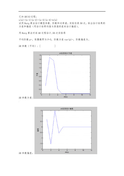
已知AR(4)过程:x(n)=(n-1)(n-2)+(n-3)(n-4)+w(n)试用Burg算法估计模型参数、阶数和功率谱。
实验仿真50次,给出估计结果的方差和偏差(用估计结果均值与真值的差来估计偏差)。
用Burg算法对该AR过程估计,50次实验得平均阶数p=,取整数即为P=5,阶数方差var(p)=,阶数偏差为。
AR参数(平均): [ ]AR参数方差:,AR参数偏差:Burg最大熵谱估计:matlab代码:u=1;while u<=50 %50次仿真实验n=10000;|w=randn(1,n);%生成零均值,方差为的白噪声w=w-mean(w);w=w/std(w);w=sqrt*w;x(1)=1+w(1);x(2)=2+w(2);x(3)=3+w(3);x(4)=4+w(4);%由ar模型生成含噪信号;for i=5:nx(i)=*x(i-1)*x(i-2)+*x(i-3)*x(i-4)+w(i);endP(1+1)=1/n*sum(x.^2);%计算预测误差功率的初始值-g(1,:)=x;f(1,:)=g(1,:);m=1;k=0;l=0;a(1,1)=1;P(1)=1;while abs(P(m+1)-P(m))/P(m)>=for j=m+1:nk=k+f(m,j)*g(m,j-1);l=l+f(m,j)^2+g(m,j-1)^2;endK(m)=-k/(1/2*l);%求反射系数a(1,1)=1;、if m>=2for j=1:m-1%计算前向预测滤波器系数a(m,j)=a(m-1,j)+K(m)*a(m-1,m-j);a(m,m)=K(m);endendP(m+1+1)=(1+abs(K(m))^2)*P(m+1);%计算预测误差功率for j=1:n%计算滤波器输出f(m+1,j)=f(m,j)+K(m)*g(m,n-1);g(m+1,j)=K(m)*f(m,j)+g(m,n-1);end(m=m+1;endM(u)=m-1;%记录每次实验的阶数u=u+1;endfor i=1:50ar=arburg(x,M(i));%估计AR系数ar_coef(i,1:length(ar))=ar;[Px,fx]=pburg(x,M(i));%估计功率谱Pxx(i,1:length(Px))=10*log10(Px');…fxx(i,1:length(fx))=fx';end%%求阶数和AR系数的方差和偏差var_p=var(M);for i=1:max(M)var_ar(i)=var(ar_coef(:,i+1));endbias_p=mean(M)-4;ar_r(max(M))=0;ar_r(1)=;ar_r(2)=;ar_r(3)=;ar_r(4)=;for i=1:max(M)`mean_ar(i)=mean(ar_coef(:,i+1));bias_ar(i)=mean(ar_coef(:,i+1))-ar_r(i);end%%50次实验功率谱平均for i=1:length(Pxx(1,:))mean_Pxx(i)=mean(Pxx(:,i));end%%作图plot(fxx(1,:),mean_Pxx);%作功率谱图title('burg最大熵估计功率谱'); xlabel('频率');ylabel('功率谱密度');》figure(2);plot(var_ar);%AR系数估计方差title('AR系数估计方差');xlabel('AR(n)');ylabel('方差');figure(3);plot(bias_ar);%AR系数估计偏差title('AR系数估计偏差');xlabel('AR(n)');ylabel('偏差');disp('阶数方差:');disp(var_p);disp('阶数偏差:');disp(bias_p);disp('AR系数:');disp(mean_ar);。
基于AR模型的功率谱估计

基于AR模型的功率谱估计邢务强;钮金鑫【摘要】A self-correlation method and Burg method based on AR model are usually used in the modern PSD for better simulating and computing the power spectrum. Through simulation, PSD curve is acquired by three methods. The results show that Burg method has good performance in the spectral resolution. An appropriate sampling point should be selected to determine the model order. At the same time, the principle of order selection is given.%为了更好地模拟计算功率谱,采用了现代功率谱估计中常用的基于AR模型的自相关法和Burg法,通过仿真给出了估计出的功率谱曲线,结果表明,Burg算法在谱分辨率方面有着良好的性能.选择合适的采样点数来确定模型阶数,给出阶数选择的原则.【期刊名称】《现代电子技术》【年(卷),期】2011(034)007【总页数】3页(P49-51)【关键词】AR模型;自相关法;Burg算法;阶数选择【作者】邢务强;钮金鑫【作者单位】西安邮电学院理学院,陕西西安710121;西安邮电学院通信工程学院,陕西西安710121【正文语种】中文【中图分类】TN911-340 引言所谓谱估计或功率谱估值,就是用已观测到的一定数量的样本数据估计一个平稳随机信号的功率谱。
功率谱估计分为两大类,一类是非参数化方法(又叫经典谱估计法),另一类是参数化方法(又叫模型法估计)。
精选-数字信号处理-谱估计基础及仿真分析
谱估计基础及仿真分析0引言 现代信号分析中,对于常见的具有各态历经的平稳随机信号,不可能用清楚的数学关系式来描述,但可以利用给定的N 个样本数据估计一个平稳随机信号的功率谱密度叫做功率谱估计(PSD)。
它是数字信号处理的重要研究内容之一。
功率谱估计可以分为经典功率谱估计(非参数估计)和现代功率谱估计(参数估计)。
功率谱估计在实际工程中有重要应用价值,如在语音信号识别、雷达杂波分析、波达方向估计、地震勘探信号处理、水声信号处理、系统辨识中非线性系统识别、物理光学中透镜干涉、流体力学的内波分析、太阳黑子活动周期研究等许多领域,发挥了重要作用。
一 相关的数学基础 1.1 概率论:1.1.1多维高斯分布高斯分布公式:22()2()x p x μσ--=(1)3σ准则为:(,)σσ-内68.26%;2σ:95.44%;3σ:99.74%。
向量的形式的公式为:11/21/211()exp[()()](2)||2T x xx x N xx p x x C x C μμπ--=---vv v v v (2) 其中[()()]Txx x x C E x x μμ=--v v v v;[]{[[]][[]]}xx ij i i j j C E x E x x E x =--(3)1.1.2 mont-carlo 仿真1ln ,(0,1)y u u λ=-∈为指数分布,y σ=1.2 随即过程平稳随即过程:多维联合概率密度和时间起点无关,狭义的平稳。
数字特征: ()[()]t E x t μ=相关函数:1212(,)[()()]xx r t t E x t x t =(4) 协方差:121122(,){[()()][()()]}xx x x C t t E x t t x t t μμ=--(5) 广义的平稳:1221(,)()()xx xx xx r t t r t t r τ=-=,12(,)()xx xx C t t C τ=(6)各态历经性:时间平均代替集平均。
功率谱估计Levinson 递推法和 Burg 法

数字信号处理实验报告姓名: 学号: 日期:2015.12.141. 实验任务信号为两个正弦信号加高斯白噪声,各正弦信号的信噪比均为10dB ,长度为N ,信号频率分别为1f 和2f ,初始相位021==ϕϕ,取2.01=s f f ,s f f 1取不同的数值:0.3,0.25。
s f 为采样率。
(1)分别用 Levinson 递推法和 Burg 法进行功率谱估计,并分析改变数据长度、模型阶数对谱估计结果的影响。
(2)当正弦信号相位、频率、信噪比改变后,上述谱估计的结果有何变化?并作分析说明。
2. 原理分析2.1 现代谱估计中的参数建模根据参数模型来描述随机信号的方法,我们可以知道,如果能确定信号()x n 的信号模型,根据信号观测数据求出模型参数,系统函数用()z H 表示,模型输入白噪声,其方差为2w σ,信号的功率谱用下式求出:()()22iww jw xx e H e P σ=按照这种求功率谱的思路,功率谱估计可分为三个步骤: (1)选择合适的信号模型;(2)根据()n x 有限的观测数据,或者它的有限个自相关函数的估计值,估计模型的参数;(3)计算墨香的输出功率谱。
其中以(1)、(2)两步最为关键。
按照模型的不同,谱估计的方法有许多种,它们共同的特点是对信号观测区以外的数据不假设为0,而先根据信号观测数据估计模型参数,按照求模型输出功率的方法估计信号功率谱,回避了数据观测区以外的数据假设问题。
下面分析AR 谱估计的两种方法:自相关法——列文森(Levenson )递推法和伯格(Burg )递推法。
这两种方法均为已知信号观测数据,估计功率谱,两者共同特点是由信号观测数据求模型系数时采用信号预测误差最小的原则。
对于长记录数据,这些方法的估计质量是相似的,但对于短记录数据,不同方法之间存在差别。
2.2 自相关法——列文森(Levenson )递推法自相关法的出发点是选择AR 模型参数使预测误差功率最小,预测误差功率为()()()21211∑∑∑∞-∞==∞-∞=-+==n pi pi n i n x a n x Nn e Nρ假设信号()x n 的数据区在01n N ≤≤-范围,有P 个预测系数,N 个数据经过冲激响应为()0,1,pi a i p =的滤波器,输出预测误差()e n 的长度为N p +,因此应用下式计算:()()()210121011∑∑∑-+==-+=-+==P N n pi pi P N n i n x a n x Nn e Nρ()e n 的长度长于数据的长度,上式中数据()x n 的两端需补充零点,相当于对无穷长的信号加窗处理,得到长度为N 的数据。
Yule-Walker法和Burg法对信号进行谱估计的Matlab仿真
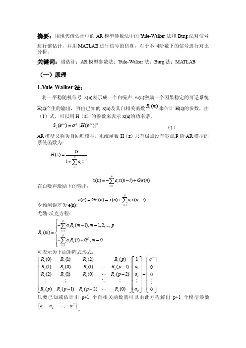
摘要:用现代谱估计中的AR 模型参数法中的Y ule-Walker 法和Burg 法对信号进行谱估计,并用MATLAB 进行信号的仿真,对于不同阶数下的信号进行对比分析。
关键词:谱估计;AR 模型参数法;Yule-Walker 法;Burg 法;MA TLAB (一)原理 1.Y ule-Walker 法:将一平稳随机信号x(n)表示成一个白噪声w(n)激励一个因果稳定的可逆系统H(z)产生的输出,再由已知的x(n)及其自相关函数()x R m 来估计H(z)的参数,由(1)式,可以用H (z )的参数来表示x(n)的功率谱。
22()|()|jw jw x S e H e σ= (1) AR 模型又称为自回归模型,系统函数H (z )只有极点没有零点,P 阶AR 模型的系统函数为:1()1pii i G H z a z -==+∑在白噪声激励下的输出:1()()()pi i x n a x n i Gw n ==--+∑令预测误差为e(n):1()()()()pi i e n Gw n x n a x n i ===+-∑尤勒-沃克方程:121(1),1,2,...,()(),0pi x i x pi x i a R m m p R m a R i G m ==⎧--=⎪⎪=⎨⎪-+=⎪⎩∑∑可表示为下面矩阵式形式:2121(0)(1)(2)()(1)(0)(1)(1)0(2)(1)(0)(2)0()(1)(2)(0)0x x x x x x x x x x x x p x x x x R R R R p a R R R R p a R R R R p a R p R p R p R σ⎡⎤⎡⎤⎡⎤⎢⎥⎢⎥⎢⎥-⎢⎥⎢⎥⎢⎥⎢⎥⎢⎥⎢⎥-=⎢⎥⎢⎥⎢⎥⎢⎥⎢⎥⎢⎥⎢⎥⎢⎥⎢⎥--⎣⎦⎣⎦⎣⎦只要已知或估计出p+1个自相关函数就可以由此方程解出p+1个模型参数{}21,2,,aa σ 。
Levinson-Durbin 递推算法是解尤勒-沃克方程的快速有效的算法,这种算法利用方程组系数矩阵所具有的一系列好的性质,使运算量大大减少。
AR模型论文
摘要:本文在AR模型(自回归模型)功率谱估计方法的基础上,对其在抗干扰领域中的应用进行了研究,提出了自适应滤除干扰信号的方案,并对该方案进行了DSP实现。
实验结果表明,该方案在自适应去除多个干扰信号方面是行之有效的。
关键词:功率谱估计;自回归模型;抗干扰;数字信号处理器DSP Realization of AR Model Power Spectrum Estimation in Anti-jammingJIANG Lei1,2,CHENG Ren2 ,LIU Yi-de2(1.Electronics and Information Institute, Northwest Polytechnical University, Xi'an 710072,China;2.Telecommunication Engineering Institute, Air Force Engineering University,Xi'an 710077,China)Abstract:The application of AR model power spectrum esti mation in the field of anti-jamming is studied. The scheme of adaptiv ely filtering jamming signal is also proposed and is realized based on DSPs. The experiment result shows that this scheme is effective t o filter multi-jamming signal.Keywords:Power spectrum estimation;AR model;Anti-jamming;DSP一、引言参数模型功率谱估计方法较经典功率谱估计方法无论是在方差性能还是在分辨率方面都有明显的优势,因而成为现代谱估计技术的主要内容,被广泛地应用到各个领域。
自相关法和Burg法在AR模型功率谱估计中的仿真研究
现代谱估计。由于经典谱估计 中将数据工作 区以 外 的未知数 据假 设 为 零 , 相 当于 数据 加 窗 , 这 导致 分辨率降低和谱估计不稳定。现代谱估计则不再 简单地将观察 区外 的未知假设为而零 , 而是先将信 号的观测数据估计模型参数, 按照求模型输出功率 的方法估计信号功率谱 , 回避了数据观测区以外的 数据假设 问题 。可以看 出现代谱估计 性能优于经
解A R模 型参 数 。
单位冲激 响应加 白噪声 的平稳信 号序列 ( ) 来 n, 估计其 A R模型参数 。
参数提取时 , 用 M tb工具箱 中的信号处 利 aa l
理中的 l i o e v n函数 和 a u ss rr b g函数来 分别进行 自 相 关算 法 和 B r 法 的 A ug算 R模 型 参 数 估 计 , 果 结
- 2 or
0 0
:
●
r2 r 1 x ) ) r0 … rP 2 0 2 ( ( x ) ( 一) 口 (
j j
A R模型的功率谱估计仿真研究及比较两种算法 。
r() r( 1 xP xP一 )
( 2 … P- )
r() J a x0 Lp
_
维普资讯
3 2
计算机与数字工程
第3 5卷
自相关 法 和 B r 法 在 A ug R模 型功 率 谱 估 计 中 的仿 真研 究
姚 文俊
( 中南 民族大学电子信息工程学 院 武汉 40 7 ) 3 04
摘
要 介 绍功率谱 估计和常用的基于 A R模型 的 自 相关法和 Br算 法 , u g 通过仿真 比较这两种算法使用 和优 缺点 。
维普资讯
第3 5卷( 0 7 第 1 2 0 ) O期
(完整版)功率谱估计性能分析及Matlab仿真
功率谱估计性能分析及Matlab 仿真1 引言随机信号在时域上是无限长的,在测量样本上也是无穷多的,因此随机信号的能量是无限的,应该用功率信号来描述。
然而,功率信号不满足傅里叶变换的狄里克雷绝对可积的条件,因此严格意义上随机信号的傅里叶变换是不存在的。
因此,要实现随机信号的频域分析,不能简单从频谱的概念出发进行研究,而是功率谱[1]。
信号的功率谱密度描述随机信号的功率在频域随频率的分布。
利用给定的N 个样本数据估计一个平稳随机信号的功率谱密度叫做谱估计。
谱估计方法分为两大类:经典谱估计和现代谱估计。
经典功率谱估计如周期图法、自相关法等,其主要缺陷是描述功率谱波动的数字特征方差性能较差,频率分辨率低。
方差性能差的原因是无法获得按功率谱密度定义中求均值和求极限的运算[2]。
分辨率低的原因是在周期图法中,假定延迟窗以外的自相关函数全为0。
这是不符合实际情况的,因而产生了较差的频率分辨率。
而现代谱估计的目标都是旨在改善谱估计的分辨率,如自相关法和Burg 法等。
2 经典功率谱估计经典功率谱估计是截取较长的数据链中的一段作为工作区,而工作区之外的数据假设为0,这样就相当将数据加一窗函数,根据截取的N 个样本数据估计出其功率谱[1]。
2.1 周期图法( Periodogram )Schuster 首先提出周期图法。
周期图法是根据各态历经的随机过程功率谱的定义进行的谱估计。
取平稳随机信号()x n 的有限个观察值(0),(1),...,(1)x x x n -,求出其傅里叶变换10()()N j j n N n X e x n e ωω---==∑然后进行谱估计21()()j N S X e Nωω-= 周期图法应用比较广泛,主要是由于它与序列的频谱有直接的对应关系,并且可以采用FFT 快速算法来计算。
但是,这种方法需要对无限长的平稳随机序列进行截断,相当于对其加矩形窗,使之成为有限长数据。
同时,这也意味着对自相关函数加三角窗,使功率谱与窗函数卷积,从而产生频谱泄露,容易使弱信号的主瓣被强信号的旁瓣所淹没,造成频谱的模糊和失真,使得谱分辨率较低[1]。
基于AR模型的Burg算法功率谱估计

三种功率谱估计方法性能研究1.前言:我们已经知道一个随机信号本身的傅里叶变换并不存在,因此无法像确定性信号一样用数字表达式来精确表达它,而只能用各种统计平均量来表征它. 其中,自相关函数最能完整地表它他的统计平均量值.而一个随机信号的功率谱密度正是自相关函数的傅里叶变换,可以用功率谱密度来表征它的统计平均谱密度(PSD). 跟据维纳辛钦定理,广义平稳随机过程的功率谱是自相关函数的傅里叶变换,它取决于无数多个自相关函数值. 但对于许多实际应用中,可资利用的观测数据往往是有限的,所以要准确计算功率谱通常是不可能的.比较合理的目标是设法得到功率谱的一个好的估值,这就是功率谱估计. 也就是说,功率谱估计是根据平稳随机过程的有限个观测值,来估计该随机过程的功率谱密度.功率谱估计的评价指标包括客观度量和统计度量. 在客观度量中,谱分析特性是一个主要指标.谱分析是指估计普对真实谱中两个靠的很近的谱峰的分辨能力.统计度量是指估计的偏差,方差,均方误差,一致性等评价指标.但需要注意的是,对统计特性的分析方法只适用于长数据记录.所以,利用统计度量对不同的谱估计方法进行比较是不妥当的,只能用来对某种谱估计方法进行描述,并且一般只用来描述古典谱估计方法,因为现代谱估计方法往往用于短数据情况.功率谱估计可以分为经典谱估计(非参数估计)和现代谱估计(参数估计)。
通常将傅里叶变换为理论基础的谱估计方法叫做古典谱估计或经典谱估计;把不同于傅里叶分析的新的谱估计方法叫做现代谱估计或近代谱估计.前者主要有周期图法,自相关法及其改进方法. 现代功率谱估计方法主要有基于参数模型的自相关法、Burg 算法、改进的协方差方法等,基于非参数模型的MUSIC 算法、特征向量方法等。
本文选取比较有代表性周期图法, Burg 算法、Yule-Wallker 法(自相关法)算法进行计算机仿真,通过仿真发现了这些算法各自的优缺点,并进行归纳总结。
2三种算法的基本理论2.1 周期图法周期图法又称直接法,其具体步骤如下:第一步: 由获得的N 点数据构成的有限长序列()x Nn 直接求傅里叶变换,得频谱()x i N e ω,即()()-1-=0x =N i i N Nn ex n eωω∑ (1)第二步: 取频谱幅度的平方,并除以N,以此作为对()x n 的真实功率谱()i x S eω的估计,即()()21ˆ=i i xN S e X eNωω(2)综上所述,先用FFT 求出宿疾随机离散信号N 点的DFT ,再计算幅频特性的平方,然后除以N ,即得出该随机信号得功率谱估计。
AR过程的线性建模与功率谱估计

AR 过程的线性建模与功率谱估计一、实验内容:AR 过程的线性建模与功率谱估计。
考虑AR 过程:()(1)(1)(2)(2)(3)(3)(4)(4)(0)()x n a x n a x n a x n a x n b v n =-+-+-+-+()v n 是单位方差白噪声。
(a) 取b (0)=1, a (1)=2.7607, a (2)=-3.8106, a (3)=2.6535, a (4)=-0.9238,产生x (n )的N =256个样点。
(b) 计算其自相关序列的估计ˆ()x rk ,并与真实的自相关序列值相比较。
(c) 将ˆ()x rk 的DTFT 作为x (n )的功率谱估计,即: 1211ˆˆ()()|()|N j jk j xx k N P e rk e X e Nωωω--=-+==∑。
(d) 利用所估计的自相关值和Yule-Walker 法(自相关法),估计(1), (2), (3), (4)a a a a 和(0)b 的值,并讨论估计的精度。
(e) 用(d)中所估计的()a k 和(0)b 来估计功率谱为:2241|(0)|ˆ()1()j xjk k b P e a k e ωω-==+∑。
(f) 将(c)和(e)的两种功率谱估计与实际的功率谱进行比较,画出它们的重叠波形。
(g) 重复上面的(d)~(f),只是估计AR 参数分别采用如下方法:(1) 协方差法;(2) Burg 方法;(3) 修正协方差法。
试比较它们的功率谱估计精度。
二、实验结果及分析问题一:取b (0)=1, a (1)=2.7607, a (2)=-3.8106, a (3)=2.6535, a (4)=-0.9238,产生x (n )的N =256个样点。
计算其自相关序列的估计ˆ()x rk ,并与真实的自相关序列值相比较。
思路:计算真实的自相关值时,采用逆Levinson-Durbin 递归方法,由a 、b 参数得到(0)x r ,(1)x r ,,()x r p ,其中p 为滤波器的阶数,再采用公式()()()1px p x l r k a l r k l ==-∑外推得到kp 的自相关值;结果分析:仿真参数设置:采样点数为256自相关序列的估计ˆ()x rk 与真实自相关序列值的比较见图1,由图可知估计值与真实值存在一定的误差,但整体变化趋势相差不大。
基于齿轮箱故障诊断的AR模型中Burg法的优化
, 此,
广高压变频调速节
的
。
冷却方式
风道方式
空调方式
空水
方式
系统 能 (自 身 )
13.5 k W 13.5 k W 13.5 k W
空调 耗能
一 30 kW
空水机 组 一 一 40 kW
纯水机 组 一 一 一
水
方式
4.5 k W
一
5.5 k W
注:电费按每年8 个月计算,单价为0 . 3 元/k W *1 。
合计
13.5 k W 43.5 k W 53.5 k W
10 k W
电费
2.33万 元 / 年 7.51万 元 / 年 9.24 万 元 / 年 1.72 万 元 / 年
收 稿 日 期 =2018- 06- 28
作 者 简 介 :盛 佳 (988—),男 ,山西人,工程师,
从事电厂D C S 的
, 组态调
数 估 计 而 来 ,由 于 每 阶 的 计 算 都 存 在 预 测 误 差 ,导 致 累 积 误 差
越 来越大。为减小这种累积误差,本 文 对 式 (3)、(4)中)阶前后
向 、后 向 预 测 误 差 进 行 加 权 运 算 ,从 而 提 高 估 计 精 度 。它们分别
从 减 小 估 计 参 数 的 误 差 和 减 小 前 后 向 的 误 差 角 度 入 手 ,实现 对Burg法的优化。
在 进 行 参 数 估 计 计 算 时 ,每一 阶 的 参 数 都 是 从 前 一 阶 参
(4)
在 式 (2 ) 中对" 求#_的
并 为0,求得反射系数
2017年 10月 1 0 日一3 0 日,平 均 负 荷 为 243 M W ,变频运行 方 式 。通 过 插 入 查 找 法 ,节电率为3 4 . 8 3 % ,平均节电量为每小 时3 081.83 kW.li,总节电量为 1 479 278.4 kW.li。对 比 2017年 负 荷 并 预 测 2018年 机 组 运 行 小 时 情 况 ,预 算 全 年 节 电 量 约 为 2 500万k W *1 ,年节电费约750万 元 。
振动信号AR模型谱估计算法研究中期报告(可编辑)

振动信号AR模型谱估计算法研究中期报告毕业设计(论文)中期报告题目:振动信号AR模型谱估计算法研究系别电子信息系专业通信工程班级姓名学号导师2013年3月23日1. 设计(论文)进展状况1.1 主要研究内容及方案本课题的名称是振动信号AR模型谱估计算法研究。
本课题将对AR模型功率谱估计算法进行研究并设计一套仿真程序,在此基础上,基于实测振动信号进行算法性能分析,为科研项目“汽轮机振动在线监测系统”中振动信号频谱分析的实现提供基础,主要内容如下:1 了解功率谱估计的基本理论、概念、应用及实现方式;2 对AR模型功率谱估计算法进行研究;3 基于Matlab环境编程仿真实现算法;4 编写图形用户界面,并与算法程序结合,构成一套完整的仿真程序;5 将实现的算法应用于实测汽轮机振动信号的谱估计;6 对算法效果及性能进行分析。
课题的研究按以下的过程进行:1 首先对振动信号AR模型谱估计算法进行深入研究。
AR模型又称为自回归模型,建立如下的信号模型:假定所观测的数据是由一个均方误差为的零均值白噪声序列wn激励一个全极点的线性时不变离散时间系统Hz得到的。
用差分方程表示为1其中,p是AR模型的阶数,是p阶AR模型的参数.将该模型记为ARp,它的系统转移函数为2在功率谱估计中,若观测的数据是平稳随机过程,则该系统的输入wn也可认为是平稳的,因而根据线性系统对平稳随机信号的响应理论可得观测数据的功率谱为 3由上式可知,利用AR模型进行功率谱估计的实质是求解模型系数和的问题。
2 在算法研究的基础之上,用Matlab对其进行编程实现,并以模拟的信号对算法进行测试。
3 利用MATLAB的GUI编写图形用户界面程序,形成一套AR模型谱估计算法仿真程序。
4 基于实测的汽轮机振动信号对AR模型谱估计算法性能进行分析。
5 在对比的基础上,发现并提出算法的改进方向。
1.2 设计进展情况从开题到中期,课题的进展情况如下:1 查阅了课题实现的相关文献及资料,主要文献包括:《AR模型功率谱估计及MATLAB实现》、《功率谱估计及其MATLAB仿真》、《基于AR模型的功率谱估计》等等,了解了功率谱估计的的本理论、概念、应用及实现方式,着重分析了AR模型谱估计算法及其参数求解。
- 1、下载文档前请自行甄别文档内容的完整性,平台不提供额外的编辑、内容补充、找答案等附加服务。
- 2、"仅部分预览"的文档,不可在线预览部分如存在完整性等问题,可反馈申请退款(可完整预览的文档不适用该条件!)。
- 3、如文档侵犯您的权益,请联系客服反馈,我们会尽快为您处理(人工客服工作时间:9:00-18:30)。
AR 模型的功率谱估计BURG 算法的分析与仿真一.引言现代谱估计法主要以随机过程的参数模型为基础,也可以称其为参数模型方法或简称模型方法。
现代谱估计技术的研究和应用主要起始于20世纪60年代,在分辨率的可靠性和滤波性能方面有较大进步。
目前,现代谱估计研究侧重于一维谱分析,其他如多维谱估计、多通道谱估计、高阶谱估计等的研究正在兴起,特别是双谱和三谱估计的研究受到重视,人们希望这些新方法能在提取信息、估计相位和描述非线性等方面获得更多的应用。
现代谱估计从方法上大致可分为参数模型谱估计和非参数模型谱估计两种。
基于参数建摸的功率谱估计是现代功率谱估计的重要内容,其目的就是为了改善功率谱估计的频率分辨率,它主要包括AR 模型、MA 模型、ARMA 模型,其中基于AR 模型的功率谱估计是现代功率谱估计中最常用的一种方法,这是因为AR 模型参数的精确估计可以通过解一组线性方程求得,而对于MA 和ARMA 模型功率谱估计来说,其参数的精确估计需要解一组高阶的非线性方程。
在利用AR 模型进行功率谱估计时,必须计算出AR 模型的参数和激励白噪声序列的方差。
这些参数的提取算法主要包括自相关法、Burg 算法、协方差法、 改进的协方差法,以及最大似然估计法。
本章主要针对采用AR 模型的两种方法:Levinson-Durbin 递推算法、Burg 递推算法。
实际中,数字信号的功率谱只能用所得的有限次记录的有限长数据来予以估计,这就产生了功率谱估计这一研究领域。
功率谱的估计大致可分为经典功率谱估计和现代功率谱估计,针对经典谱估计的分辨率低和方差性能不好等问题提出了现代谱估计,AR 模型谱估计就是现代谱估计常用的方法之一。
信号的频谱分析是研究信号特性的重要手段之一,通常是求其功率谱来进行频谱分析。
功率谱反映了随机信号各频率成份功率能量的分布情况,可以揭示信号中隐含的周期性及靠得很近的谱峰等有用信息,在许多领域都发挥了重要作用。
然而,实际应用中的平稳随机信号通常是有限长的,只能根据有限长信号估计原信号的真实功率谱,这就是功率谱估计。
二.AR 模型的构建假定u(n)、x(n)都是实平稳的随机信号,u(n)为白噪声,方差为,现在,我们希望建立AR 模型的参数和x(n)的自相关函数的关系,也即AR 模型的正则方程(normal equation)。
由)}()]()({[)}()({)(1n x m n u k m n x E m n x n x E m pk k xa r++-+-=+=∑=∑=++-+-=pk xn x m n u E n x k n m x E m r1)}()({)}()({)()()()(1m k m m r r a rxu x pk k x+--=∑= (1)由于u(n)是方差为的白噪声,有)()()(})()()({)(22m h k m k h k n u k h m n u E m k k xu r -=+=-+=∑∑∞=∞=σσδ⎩⎨⎧=≠=-000)}()({2m m m n x n u E σ(2)由Z 变换的定义,,当时,有h(0)=1。
综合(1)及(2)两式,⎪⎪⎩⎪⎪⎨⎧=-≥--=∑∑==0)(1)()(121m k m k m m pk x k pk x k x r a r a r σ (3) 在上面的推导中,应用了自相关函数的偶对称性。
上式可写成矩阵式:⎥⎥⎥⎥⎥⎥⎦⎤⎢⎢⎢⎢⎢⎢⎣⎡=⎥⎥⎥⎥⎥⎥⎦⎤⎢⎢⎢⎢⎢⎢⎣⎡⎥⎥⎥⎥⎥⎥⎦⎤⎢⎢⎢⎢⎢⎢⎣⎡----0001)0()2()1()()2()0()1()2()1()1()0()1()()2()1()0(221x x x x x x x x x x x x x x x x σa a a r r r r r r r r r r r r r r r r p p p p p p p (4) (4)上述两式即是AR 模型的正则方程,又称Yule-Walker 方程。
系数矩阵不但是对称的,而且沿着和主对角线平行的任一条对角线上的元素都相等,这样的矩阵称为Toeplitz 矩阵。
若x(n )是复过程,那么,系数矩阵是Hermitian 对称的Toeplitz 矩阵。
(4)式可简单地表示为式中,为全零列向量,R 是的自相关矩阵。
可以看出,一个p 阶的AR 模型共有p+1个参数,即,只要知道x(n)的前p+1个自相关函数,由(1),(2)及(3)式的线性方程组即可求出这p+1个参数,即可求出x(n)的功率谱。
三.AR 模型阶数的选择AR 模型的阶次p 一般事先是不知道的,需要事先选定一个稍大的值,在递推的过程中确定。
在使用Levinson 递推时,可以给出由低阶到高阶的每一组参数,且模型的最小预测误差功率是递减的。
直观上讲,当达到所指定的希望值,或是不再发生变化时,其时的阶次即是应选的正确阶次。
因为是单调下降的,因此,的值降到多少才合适,往往不好选择。
为此,有几个不同的准则被提出,其中较常用的两个是:最终预测误差准则: (1)(2) 信息论准则:式中N 为数据的长度,当阶次k 由1增加时,FPE(k)和AIC(k)都将在某一个k 处取得极小值。
将此时的k 定为最合适的阶次p 。
在实际运用时发现,当数据较短时,它们给出的阶次偏低,且二者给出的结果基本上是一致的。
应该指出,上面两式仅为阶次的选择提供了一个依据,对所研究的某一个具体信号x(n),究竟阶次取多少为最好,还要在实践中所得到的结果作多次比较后,予以确定。
四.Burg 算法的理论分析Burg 算法是较早提出的建立在数据基础上的AR 系数求解的有效算法[7]。
其特点是: (1) 令前后向预测误差功率(5)为最小。
(2) 和的求和范围从p至N-1,即,前后都不加窗,这时(6)在上式中,阶次m由1至p时,(7)下式的递推关系,即(8)(9)(10)式中。
这样,(5)式的仅是反射系数的函数。
在阶次m时,令相对为最小,即可估计出反射系数。
将(6)、(7)及(8)式代入(5)式,令=∂∂mfb kρ,可得使为最小的为式中。
按此式估计出的满足。
按上式估计出后,在阶次m时的AR模型系数仍然由Levinson算法递推求出(11)(12)式中。
上面三式是假定在第(m-1)阶时的AR参数已求出。
Burg算法的递推步骤是:(1)由初始条件,再由(11)式求出;(2)由得m=1时的参数:;(3)由求出,再估计;(4)依照(11)、(12)式的Levinson递推关系,求出m=2时的及。
(5)重复上述过程,直到m=p,求出了所有阶次时的AR参数。
上述递推过程是建立在数据基础上的,避开了先估计自相关函数的这一步。
若定义:可以证明可以由和递推计算:这样,可以有效地提高计算速度。
五.Burg 算法的MATLAB 仿真%Burg 算法 %生成信号xn f1=30;f2=60; f=[f1;f2]; A=[1 2];Fs=200; % 取样频率 n=0:1/Fs:1;x=A*sin(2*pi*f*n);%生成噪声n 和被污染的信号xn randn('state',0);n=0.1*randn(size(n)); xn=x+n; % 设置参数 order=10; nfft=512; % Burg 算法[Pxx1,f]=pburg(xn,order,nfft,Fs); Pxx1=10*log10(Pxx1); subplot(1,1,1),plot(f,Pxx1); xlabel(‘频率(Hz)’);ylabel(‘功率谱密度(dB/Hz)’); title (‘Burg 算法(阶数=15)’); grid on;102030405060708090100-50-45-40-35-30-25-20-15-10-50频率(Hz)功率谱密度(d B /H z )Burg 算法(阶数=10)图1 阶数为10,噪声为0.1时的Burg 算法得到的仿真结果0102030405060708090100-30-25-20-15-10-5频率(Hz)功率谱密度(d B /H z )Burg 算法(阶数=10)图2 阶数为10,噪声为1时的Burg 算法得到的仿真结果102030405060708090100-50-45-40-35-30-25-20-15-10-50频率(Hz)功率谱密度(d B /H z )Burg 算法(阶数=15)图3 阶数为15,噪声为0.1时的Burg 算法得到的仿真结果仿真结果:Burg 算法得到的谱线分辨率很高,谱的波动性不大,能清晰的分辨出两个频率值,且没有出现假峰。
从图中可以看出在两个阶数不同的情况下都能很好的分辨出两个频率的峰值,说明增加阶数并没有增大频率分辨率,而增加的阶数反而使计算量加大。
相比较Levinson-Durbin 算法而言,Burg 算法因为没有使用自相关估计法,结果与真实值更加接近,而且可以进行外推,所以Burg 算法要比Levinson-Durbin 算法要好。
当噪声方差加大为原来的10倍时,还能比较清楚的分辨出两个频率值如图2所示,说明Burg 算法的抗干扰能力比较好。
六.总结参数建模谱估计方法是现代谱估计的重要内容,AR 模型谱估计隐含着数据和自相关函数的外推,其长度可能超过给定的长度,分辨率不受信源信号长度的限制,所以现代谱估计研究主要是用基于AR 模型的方法估计功率谱,这是经典谱估计无法做到的。
通过实践,AR模型的Burg法也存在问题:(1)计算量大;(2)信号起始相位变动可导致谱线偏移和分裂;(3)低信噪比可导致谱分辨率下降、谱线偏移、甚至丢失;(4)阶数的确定还没有找到确切有效准则。
这些是AR模型估计的不足之处。
功率谱估计是信息学科中的研究热点。
现代谱估计主要是针对经典谱估计(周期图和自相关法)的分辨率低和方差性能不好的问题而提出的。
其内容极其丰富,涉及的学科和领域也相当广泛,按是否有参数大致可分为参数模型估计和非参数模型估计,前者有AR模型、MA模型、ARMA模型、PRONY指数模型等;后者有最小方差方法、多分量的MUSIC方法等。
从信号的特征来分,在这之前所说的方法都是对平稳随机信号而言,其谱分量不随时间变化。
对非平稳随机信号,其谱是时变的,近十五年,以Wigner 分布为代表的时频分析引起了人们广泛的兴趣,形成了现代谱估计的一个新的研究领域。