哈工大机电控制系统 大作业一
哈工大_机电系统控制基础实验_实验一
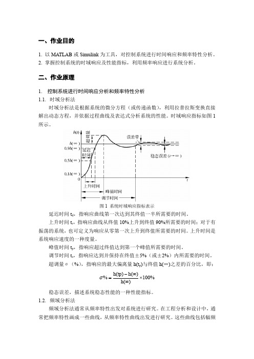
姓名:学号:课程名称:机电系统控制基础实验实验序号: 1 实验日期:实验室名称:同组人:实验成绩:总成绩:教师评语:教师签字:年月日机电系统控制基础原理性仿真实验一、实验目的通过仿真实验,掌握在典型激励作用下典型机电控制系统的时间响应特性,分析系统开环增益、系统阻尼、系统刚度、负载、无阻尼自振频率等机电参数对响应、超调量、峰值时间、调整时间、以及稳态跟踪误差的影响;掌握系统开环传递函数的各参数辨识方法,最后,学会使用matlab 软件对机电系统进行仿真,加深理解系统动态响应特性与系统各参数的关系。
二、实验原理1.一阶系统的单位脉冲响应惯性环节(一阶系统)单位脉冲响应simulink 实现图,如图2-1 所示(a)可观测到输出曲线(b)输入、输出曲线均可观测到图2-1 惯性环节(一阶系统)单位脉冲响应simulink 实现图2.一阶系统的单位阶跃响应一阶系统的单位阶跃响应simulink 实现图如图2-2 所示。
图2-2 一阶系统的单位阶跃响应simulink 实现图3.二阶系统的单位脉冲响应二阶系统的单位脉冲响应simulink 实现图,如图2-3 所示。
图2-3 二阶系统的单位脉冲响应simulink 实现图4.二阶系统的单位阶跃响应二阶系统的单位阶跃响应实验simulink 实现图如图2-4 所示。
图2-4 二阶系统的单位阶跃响应实验simulink 实现图三、实验要求1. 掌握在典型激励作用下典型机电控制系统的时间响应特性。
2. 掌握系统开环传递函数的各参数辨识方法。
3. 使用matlab 软件对机电系统进行仿真四、实验结果1. 一阶系统的单位脉冲响应Simulink 模型图如图4-1图4-1 一阶系统单位脉冲响应模型图单位脉冲函数波形图如图4-2图4-2 单位脉冲函数波形图图4-3 输出函数波形图2. 一阶系统的单位阶跃响应Simulink 模型图如图4-4图4-4一阶系统的单位阶跃响应模型图单位阶跃函数波形图如图4-5图4-5 单位阶跃函数波形图图4-6 输出函数波形3.二阶系统的单位脉冲响应Simulink 模型图如图4-7图4-7 Simulink 模型图单位脉冲函数波形图如图4-2。
哈工大自动控制原理大作业
Harbin Institute of Technology自动控制原理设计论文课程名称:自动控制原理设计题目:液压伺服系统校正院系:测控技术与仪器系班级:设计者:学号:指导教师:设计时间:哈尔滨工业大学自动控制原理大作业一、 设计任务书考虑图中所示的系统。
要求设计一个校正装置,使得稳态速度误差常数为-14秒,相位裕度为,幅值裕度大于或等于8分贝。
利用MATLAB 画出已校正系统的单位阶跃响应和单位斜坡响应曲线。
二、 设计过程1、 人工设计1)、数据计算由图可知,校正前的开环传递函数为:0222s+0.10.025(20s 1)G =0.1(s 0.14)(1)44s s s s s +=++++ 其中按频率由小到大分别含有积分环节和放大环节,-20dB/dec ;一阶微分环节,10.05/w rad s =,0dB/dec;振荡环节,22/w rad s =,-40dB/dec;稳态速度误差:0202s+0.1e ()lim (s)lim 0.025(s 0.14)ss s s sG ss s →→∞===++。
显然,此时的相位裕度和稳态速度误差都不满足要求。
为满足题目要求,可以引入超前校正,提高系统的相位裕度和稳态速度误差。
2)、校正装置传递函数 (1)、稳态速度误差常数的确定为使稳态速度误差常数为-14秒,设加入的开环放大倍数为k,加入校正装置后的稳态速度误差满足: 11e ()4k 0.025kss v ∞=== 解得K=160;将K=160带入,对应的传递函数为:0222s+0.14(20s 1)G (s)=1600.1(s 0.14)(1)44s s s s s +=++++ 则校正前(加入k=160的放大倍数后)幅值穿越频率:018.00/c w rad s =,相位裕度:o 00.1631c r =; (2)、校正装置的确定这里采用超前补偿,由前面算得k=160,故设加入的校正装置传递函数为:111G (s)T 1c aT s s +=+ 设计后要求o =50γ,则o 0-=500.163149.8369o o γγ-=;a 满足:01sin 49.83691a a -=+ 解得:a =7.33,取a =8.取1010/18.00/c w rad s w rad s =<=作为第一个转折频率,取第二个转折频率为21*80/w a w rad s ==;在伯德图上过3rad/s 处做斜率为-20dB/dec 的线。
哈工大 机电学院 数控大作业:加工中心零件加工编程

数控大作业一加工中心零件加工编程哈尔滨工业大学机电工程学院09级数控技术大作业©哈尔滨工业大学一、目的和要求本作业通过给定一台数控机床具体技术参数和零件加工工艺卡,使学生对数控机床具体参数、加工能力和加工工艺流程有直观了解和认识。
同时,锻炼学生解决实际加工问题的能力。
1.了解加工中心的具体技术参数,加工范围和加工能力;2.了解实际加工中,从零件图纸分析到制定零件加工工艺过程;3.按照加工工艺编写指定的工序的零件数控加工程序。
二、数控机床设备(1)机床结构主要由床身、铣头、横进给、升降台、冷却、润滑及电气等部分组成。
XKJ325-1数控铣床配用GSK928型数控系统,对主轴和工作台纵横向进行控制,用户按照加工零件的尺寸及工艺要求,先编成零件的加工程控,最后完成各种几何形状的加工。
(2)机床的用途和加工特点本机床适用于多品种中、小批量生产的零件,对各种复杂曲线的凸轮、孔、样板弧形糟等零件的加工效能尤为显著;该机床高速性能好,工作稳定可靠,定位精度和重复精度较高,不需要模具就能确保零件的加工精度,减少辅助时间,提高劳动生产率。
(3)加工中心的主要技术参数数控机床的技术参数,反映了机床的性能及加工范围。
表1 TH5640D立式加工中心的主要技术参数三、加工工艺制订(一)加工零件加工图1零件,材料HT200,毛坯尺寸长*宽*高为170×110×50mm,试分析该零件的数控铣削加工工艺、如零件图分析、装夹方案、加工顺序、刀具卡、工艺卡等,编写加工程序和主要操作步骤。
图1 加工零件图(二)工艺分析(1)零件图工艺分析。
该零件主要由平面,孔及外轮廓组成,平面与外轮廓的表面粗糙度要求Ra6.3,可采用铣粗—精铣方案。
(2)确定装夹方案。
根据零件的特点,加工上表面,¢60外圆及其台阶面和孔系时选用平口虎钳夹紧;铣削外轮廓时,采用一面两孔的定位方式,即以底面,¢40H和¢13孔定位。
(3)确定加工顺序。
机电系统控制技术大作业
哈尔滨工业大学工业工程系机电系统控制技术大作业班级:1008401班学号:1100800807姓名:匡野日期:2013.7.14指导教师:崔贤玉成绩:机电系统控制技术大作业要求根据PI 、PD 、PID 调节器的频率特性简述其校正的作用;以近似PID 调节器为例详述其校正的过程;最后以下题的指标要求为例详细设计校正网络及参数。
题:某单位反馈系统的开环传递函数为()11(1)(1)1060KG s s s s =++当输入速度为1rad/s 时,稳态位置误差为e ss ≤1126rad ,相位裕度,0()30c γω≥,幅值穿越频率,20c ω≥rad/s 。
(1)根据稳态精度位置误差求出系统开环放大系数原系统为I型系统,所以。
做出原系统的图,如图所示。
由图可得,错误!未找到引用源。
,错误!未找到引用源。
,原系统不稳定。
(2)选择校正方式虽然采用一级超前校正,无法实现如此大的相位超前;若采用两级超前校正,虽可以实现需要的相位超前,但响应速度将远远超出性能指标的要求,带宽过大,抗高频干扰能力变差,同时需要放大器,系统结构复杂,故不宜采用两级超前校正。
如采用串联滞后校正,虽可实现相位裕量的要求,但响应速度又不能满足要求,同时之后校正装置的转折频率必须远离错误!未找到引用源。
,则校正装置的时间常数错误!未找到引用源。
将大大增加,物理上难以实现,故也不宜采取滞后校正。
因此,现拟采用无源串联滞后-超前网络来校正。
(3)设计滞后-超前校正装置首先选择校正后系统的幅值穿越频率错误!未找到引用源。
从原系统的博德图可以看出,当错误!未找到引用源。
时,原系统的相角为错误!未找到引用源。
故选择校正后的系统幅值穿越频率错误!未找到引用源。
较为方便。
这样在错误!未找到引用源。
处,所需相位超前角应大于或等于错误!未找到引用源。
当错误!未找到引用源。
选定之后,下一步确定滞后-超前校正网络的相位滞后部分打的转折频率错误!未找到引用源。
哈工大机械原理大作业一连杆_20
Harbin Institute of Technology(一)连杆设计说明书课程名称:机械原理设计题目:连杆机构运动分析院系:机电工程学院班级:1308302设计者:吉曾纬指导教师:赵永强唐德威设计时间:2015年6月运动分析题目:如图所示机构,已知机构各构件的尺寸为AB=150mm ,β=97°,BC=400mm ,CD=300mm ,AD=320mm ,BE=100mm ,EF=230mm ,FG=400mm ,构件1的角速度为ω1=10rad/s,试求构件2上点F 的轨迹及构件5上点G 的位移、速度和加速度,并对计算结果进行分析。
一.对机构进行结构分析依题意可以将杆机构看作曲柄滑块机构和曲柄摇杆机构。
对4机构进行结构分析该机构由原动件AB (Ⅰ级组),BCD (RRR Ⅱ级杆组)和FG (RRP Ⅱ级杆组)组成。
二.建立以点A 为原点的固定平面直角坐标系A-x,y,如图所示。
三.各基本杆组的运动分析数学模型(1)原动件AB(Ⅰ级组)已知原动件AB的转角ψ1=0~2π原动件AB的角速度ω1=10rad/s原动件AB的角加速度α1=0运动副A的位置坐标xA =0 yA=0A点与机架相连,即该点速度和加速度均为0。
运动副A的速度vxA =0 vyA=0运动副A的加速度axA =0 ayA=0原动件AB长度lAB=150mm 可求出运动副B的位置坐标xB =xA+lABcosψ1yB=xA+lABsinψ1运动副B的速度vxB = vxA-ω1lABsinψ1vyB= vyA+ω1lABcosψ1运动副B的加速度a xB = a xA -ω12 l AB cos ψ1-α1l AB sin ψ 1 a yB =a yA -ω12 l AB sin ψ1+α1l AB cos ψ 1 (2) BCD (RRR Ⅱ级杆组)由(1)知B 点位置坐标、速度、加速度 运动副D 点位置坐标x D =320mm y D =0 D 点与机架相连,即该点速度和加速度均为0。
哈工大机电控制系统大作业一
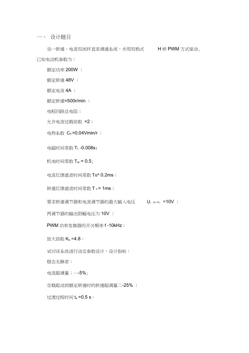
设一转速、电流双闭环直流调速系统,米用双极式H桥PWM方式驱动, 已知电动机参数为:额定功率200W ;额定转速48V ;额定电流4A ;额定转速=500r/min ;电枢回路总电阻;允许电流过载倍数=2;电势系数C e =0.04Vmin/r ;电磁时间常数T L-0.008s;机电时间常数T m= 0.5;电流反馈滤波时间常数To^ 0.2ms;转速反馈滤波时间常数T°n = 1ms;要求转速调节器和电流调节器的最大输入电压U;m =5;=10V ;两调节器的输出限幅电压为10V ;PWM功率变换器的开关频率f -10kHz;放大倍数K s=4.8。
试对该系统进行动态参数设计,设计指标:稳态无静差;电流超调量;—-5%;空载起动到额定转速时的转速超调量二-25% ;过渡过程时间t s=0.5 s。
1.计算电流和转速反馈系数电流反馈系数:U10 = 1.25(V/A )'Inom2 4转速反馈系数:*U nmCi —-10 0.02(V min /r)nn om5002.电流环的设计(1)确定时间常数电流反馈滤波时间常数T °i = 0.2ms =0.0002s ,11调制周期 T s=——0.0001s ,f 10x1000按电流环小时间常数的近似处理方法,取T 沪 T s T °i =0.0001 0.0002 = 0.0003s(2) 选择电流调节器结构电流环可按I 型系统进行设计。
电流调节器选用PI 调节器,其传递函数为皿+1 G ACR (s)二 K iNS(3) 选择调节器参数超前时间常数:j =T = 0.008s 。
电流环按超调量6^5%考虑,电流环开环增益:取 K,^^0.5,因此0.50.5K ,1666.6667Tj 0.0003于是,电流调节器的比例系数为0.008乂 8 K i = K } -1666.6667 17.7778K s1.25 4.8(4) 检验近似条件电流环的截止频率•〔= K| =1666.6667 1/s现在,3333.3333 • 1666.6667 =•⑺,满足近似条件。
哈工大机械原理大作业一连杆运动分析(02)

哈⼯⼤机械原理⼤作业⼀连杆运动分析(02)⼀.设计题⽬⼆. 结构分析与基本杆组划分1.机构的结构分析机构各构件都在同⼀平⾯内运动,活动构件数n=3 P L=4 P H=0则机构的⾃由度为: F = 3n -2P L –P H = 3×3-2×4 = 12.基本杆组划分(1)去除虚约束和局部⾃由度本机构中⽆虚约束或局部⾃由度,此步骤跳过。
(2)拆杆组。
从远离原动件(即杆1)进⾏拆分,就可以得到由杆2,3组成的RRRⅡ级杆组和Ⅰ级机构杆1。
如下图:(3)确定机构的级别由(2)知,机构为Ⅱ级机构。
三. 运动分析数学模型以A为原点建⽴坐标系,如图:原动件AB的转⾓:φ1=0--2π运动副A的位置坐标:x A=0 y A=0 运动副D的位置坐标:x D=d y D=0 则运动副B的位置坐标:x B = acosφ1 y B = asinφ1其中:t=0:0.001:2*pi;a=60;b=90;c=120;xd=d;yd=0;xb=a.*cos(t);yb=a.*sin(t);m=xd-xb;n=yd-yb;lbd=(m.^2+n.^2).^(1/2);a0=2*b.*(xd-xb);b0=2*b.*(yd-yb);c0=b.^2+lbd.^2-c.^2;dd=2*atan((b0+(a0.^2+b0.^2-c0.^2).^(1/2))./(a0+c0)); plot(dd)曲柄a=50,55,60,65红蓝绿黄b=90,c=120,d=100 t=0:0.001:2*pi; a=50;b=90;c=120;d=100;xa=0;ya=0;xd=d;yd=0;xb=a.*cos(t);yb=a.*sin(t);m=xd-xb;n=yd-yb;lbd=(m.^2+n.^2).^(1/2);a0=2*b.*(xd-xb);b0=2*b.*(yd-yb);c0=b.^2+lbd.^2-c.^2;dd=2*atan((b0+(a0.^2+b0.^2-c0.^2).^(1/2))./(a0+c0)); plot(dd,'r'); hold on;grid on;t=0:0.001:2*pi;d=100;xa=0;ya=0;xd=d;yd=0;xb=a.*cos(t);yb=a.*sin(t);m=xd-xb;n=yd-yb;lbd=(m.^2+n.^2).^(1/2);a0=2*b.*(xd-xb);b0=2*b.*(yd-yb);c0=b.^2+lbd.^2-c.^2;dd=2*atan((b0+(a0.^2+b0.^2-c0.^2).^(1/2))./(a0+c0)); plot(dd,'b'); hold on;t=0:0.001:2*pi;a=60;b=90;c=120;d=100;xa=0;ya=0;xd=d;yd=0;xb=a.*cos(t);yb=a.*sin(t);m=xd-xb;n=yd-yb;lbd=(m.^2+n.^2).^(1/2);a0=2*b.*(xd-xb);b0=2*b.*(yd-yb);c0=b.^2+lbd.^2-c.^2;dd=2*atan((b0+(a0.^2+b0.^2-c0.^2).^(1/2))./(a0+c0)); plot(dd,'g'); hold on;t=0:0.001:2*pi;a=65;b=90;c=120;d=100;xa=0;ya=0;xd=d;yd=0;xb=a.*cos(t);yb=a.*sin(t);m=xd-xb;n=yd-yb;lbd=(m.^2+n.^2).^(1/2);a0=2*b.*(xd-xb);b0=2*b.*(yd-yb);c0=b.^2+lbd.^2-c.^2;dd=2*atan((b0+(a0.^2+b0.^2-c0.^2).^(1/2))./(a0+c0)); plot(dd,'y');a=50,55,60,65红蓝绿黄2.摇杆c=105,115,125,135红蓝绿黄a=50,b=90,d=100 t=0:0.001:2*pi; a=50;b=90;d=100;xa=0;ya=0;xd=d;yd=0;xb=a.*cos(t);yb=a.*sin(t);m=xd-xb;n=yd-yb;lbd=(m.^2+n.^2).^(1/2);a0=2*b.*(xd-xb);b0=2*b.*(yd-yb);c0=b.^2+lbd.^2-c.^2;dd=2*atan((b0+(a0.^2+b0.^2-c0.^2).^(1/2))./(a0+c0)); plot(dd,'r'); hold on;grid on;t=0:0.001:2*pi;a=50;b=90;c=115;d=100;xa=0;ya=0;xd=d;yd=0;xb=a.*cos(t);yb=a.*sin(t);m=xd-xb;n=yd-yb;lbd=(m.^2+n.^2).^(1/2);a0=2*b.*(xd-xb);b0=2*b.*(yd-yb);c0=b.^2+lbd.^2-c.^2;dd=2*atan((b0+(a0.^2+b0.^2-c0.^2).^(1/2))./(a0+c0)); plot(dd,'b');t=0:0.001:2*pi;a=50;b=90;c=125;d=100;xa=0;ya=0;xd=d;yd=0;xb=a.*cos(t);yb=a.*sin(t);m=xd-xb;n=yd-yb;lbd=(m.^2+n.^2).^(1/2);a0=2*b.*(xd-xb);b0=2*b.*(yd-yb);c0=b.^2+lbd.^2-c.^2;dd=2*atan((b0+(a0.^2+b0.^2-c0.^2).^(1/2))./(a0+c0)); plot(dd,'g'); hold on;t=0:0.001:2*pi;a=50;b=90;d=100;xa=0;ya=0;xd=d;yd=0;xb=a.*cos(t);yb=a.*sin(t);m=xd-xb;n=yd-yb;lbd=(m.^2+n.^2).^(1/2);a0=2*b.*(xd-xb);b0=2*b.*(yd-yb);c0=b.^2+lbd.^2-c.^2;dd=2*atan((b0+(a0.^2+b0.^2-c0.^2).^(1/2))./(a0+c0)); plot(dd,'y');c=105,115,125,135红蓝绿黄3.连杆b=80,90,100,110红蓝绿黄a=50,c=120,d=100 t=0:0.001:2*pi; a=50;b=80;c=120;d=100;ya=0;xd=d;yd=0;xb=a.*cos(t);yb=a.*sin(t);m=xd-xb;n=yd-yb;lbd=(m.^2+n.^2).^(1/2);a0=2*b.*(xd-xb);b0=2*b.*(yd-yb);c0=b.^2+lbd.^2-c.^2;dd=2*atan((b0+(a0.^2+b0.^2-c0.^2).^(1/2))./(a0+c0)); plot(dd,'r'); hold on;grid on;t=0:0.001:2*pi;a=50;b=90;c=120;d=100;xa=0;ya=0;xd=d;yd=0;xb=a.*cos(t);yb=a.*sin(t);m=xd-xb;n=yd-yb;lbd=(m.^2+n.^2).^(1/2);a0=2*b.*(xd-xb);b0=2*b.*(yd-yb);c0=b.^2+lbd.^2-c.^2;dd=2*atan((b0+(a0.^2+b0.^2-c0.^2).^(1/2))./(a0+c0)); plot(dd,'b'); hold on;t=0:0.001:2*pi;a=50;b=100;c=120;d=100;xa=0;ya=0;xd=d;xb=a.*cos(t);yb=a.*sin(t);m=xd-xb;n=yd-yb;lbd=(m.^2+n.^2).^(1/2);a0=2*b.*(xd-xb);b0=2*b.*(yd-yb);c0=b.^2+lbd.^2-c.^2;dd=2*atan((b0+(a0.^2+b0.^2-c0.^2).^(1/2))./(a0+c0)); plot(dd,'g'); hold on;t=0:0.001:2*pi;a=50;b=110;c=120;d=100;xa=0;ya=0;xd=d;yd=0;xb=a.*cos(t);yb=a.*sin(t);m=xd-xb;n=yd-yb;lbd=(m.^2+n.^2).^(1/2);a0=2*b.*(xd-xb);b0=2*b.*(yd-yb);c0=b.^2+lbd.^2-c.^2;dd=2*atan((b0+(a0.^2+b0.^2-c0.^2).^(1/2))./(a0+c0)); plot(dd,'y');b=80,90,100,110红蓝绿黄4.机架d=85,95,105,115 红蓝绿黄a=50,b=90,c=120 t=0:0.001:2*pi; a=50;b=90;c=120;d=85;yd=0;xb=a.*cos(t);yb=a.*sin(t);m=xd-xb;n=yd-yb;lbd=(m.^2+n.^2).^(1/2);a0=2*b.*(xd-xb);b0=2*b.*(yd-yb);c0=b.^2+lbd.^2-c.^2;dd=2*atan((b0+(a0.^2+b0.^2-c0.^2).^(1/2))./(a0+c0)); plot(dd,'r'); hold on;grid on;t=0:0.001:2*pi;a=50;b=90;c=120;d=95;xa=0;ya=0;xd=d;yd=0;xb=a.*cos(t);yb=a.*sin(t);m=xd-xb;n=yd-yb;lbd=(m.^2+n.^2).^(1/2);a0=2*b.*(xd-xb);b0=2*b.*(yd-yb);c0=b.^2+lbd.^2-c.^2;dd=2*atan((b0+(a0.^2+b0.^2-c0.^2).^(1/2))./(a0+c0)); plot(dd,'b'); hold on;t=0:0.001:2*pi;d=105;xa=0;ya=0;xd=d;yd=0;xb=a.*cos(t);yb=a.*sin(t);m=xd-xb;n=yd-yb;lbd=(m.^2+n.^2).^(1/2);a0=2*b.*(xd-xb);b0=2*b.*(yd-yb);c0=b.^2+lbd.^2-c.^2;dd=2*atan((b0+(a0.^2+b0.^2-c0.^2).^(1/2))./(a0+c0)); plot(dd,'g'); hold on;t=0:0.001:2*pi;a=50;b=90;c=120;d=115;xa=0;ya=0;xd=d;yd=0;xb=a.*cos(t);yb=a.*sin(t);m=xd-xb;n=yd-yb;lbd=(m.^2+n.^2).^(1/2);a0=2*b.*(xd-xb);b0=2*b.*(yd-yb);c0=b.^2+lbd.^2-c.^2;dd=2*atan((b0+(a0.^2+b0.^2-c0.^2).^(1/2))./(a0+c0)); plot(dd,'y');d=85,95,105,115 红蓝绿黄。
哈工大机电系统控制基础大作业Matlab时域分析
《机电系统控制基础》大作业一基于MATLAB的机电控制系统响应分析哈尔滨工业大学2013年12月12日1作业题目1. 用MATLAB 绘制系统2()25()()425C s s R s s s Φ==++的单位阶跃响应曲线、单位斜坡响应曲线。
2. 用MATLAB 求系统2()25()()425C s s R s s s Φ==++的单位阶跃响应性能指标:上升时间、峰值时间、调节时间和超调量。
3. 数控直线运动工作平台位置控制示意图如下:X i伺服电机原理图如下:LR(1)假定电动机转子轴上的转动惯量为J 1,减速器输出轴上的转动惯量为J 2,减速器减速比为i ,滚珠丝杠的螺距为P ,试计算折算到电机主轴上的总的转动惯量J ;(2)假定工作台质量m ,给定环节的传递函数为K a ,放大环节的传递函数为K b ,包括检测装置在内的反馈环节传递函数为K c ,电动机的反电势常数为K d ,电动机的电磁力矩常数为K m ,试建立该数控直线工作平台的数学模型,画出其控制系统框图;(3)忽略电感L 时,令参数K a =K c =K d =R=J=1,K m =10,P/i =4π,利用MATLAB 分析kb 的取值对于系统的性能的影响。
源代码:t=[0:0.01:5];u=t;C=[25],R=[1,4,25];G=tf(C,R);[y1,T]=step(G,t);y2=lsim(G,u,t);subplot(121),plot(T,y1);xlabel('t(sec)'),ylabel('x(t)'); grid on;subplot(122),plot(t,y2);grid on;xlabel('t(sec)'),ylabel('x(t)');仿真结果及分析:源代码:t=[0:0.001:1];yss=1;dta=0.02;C=[25],R=[1,4,25];G=tf(C,R);y=step(G,t);r=1;while y(r)<yss;r=r+1;endtr=(r-1)*0.001;[ymax,tp]=max(y);tp1=(tp-1)*0.001;mp=(ymax-yss)/yss;s=1001;while y(s)>1-dta && y(s)<1+dta;s=s-1;endts=(s-1)*0.001;[tr tp1 mp ts]仿真结果及分析:C = 25ans = 0.4330 0.6860 0.2538 1.0000由输出结果知:上升时间为0.4330秒,峰值时间为0.6860秒,最大超调量为0.2538,调整时间1.0000秒。
哈工大数控大作业完美版
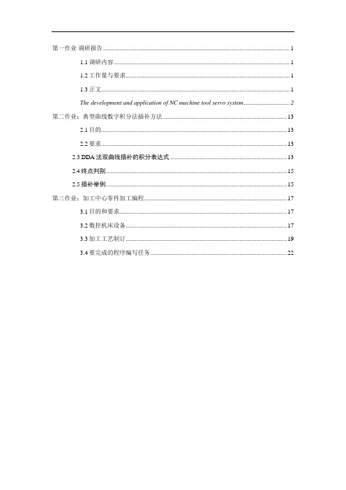
第一作业调研报告 (1)1.1调研内容 (1)1.2工作量与要求 (1)1.3正文 (1)The development and application of NC machine tool servo system (2)第二作业:典型曲线数字积分法插补方法 (13)2.1目的 (13)2.2要求 (13)2.3 DDA法双曲线插补的积分表达式 (13)2.4终点判别 (15)2.5插补举例 (15)第三作业:加工中心零件加工编程 (17)3.1目的和要求 (17)3.2数控机床设备 (17)3.3加工工艺制订 (19)3.4要完成的程序编写任务 (22)《数控技术》课程(2015)大作业院(系)专业姓名学号班号任课教师完成日期哈尔滨工业大学机电工程学院2015年5月数控大作业第一作业调研报告1.1调研内容请以课堂所学习的知识为基础,自主选择课程中所涉及的任一知识点进行调研。
可以调研知识点的发展脉络,也可以重点介绍该知识点的发展现状、争议与未来发展趋势。
请提交交独一无二的报告1.2工作量与要求1. 报告需用英文撰写,可计算机打印,也可手写,但最后封面需手工签名。
2. 格式请参照本科生毕业论文要求(见教务处网站),总字数不少于2000字。
3.在调研报告的最后,请列出参考的主要文献(英文学术刊物上正式发表的文献不少于5篇)或网址,并在正文中标注引用。
4. 如果出现雷同,两位同学均无成绩。
1.3正文The development and application of NC machine tool servo system Since the invention of NC machine tool in 1950s, servo system has been the indispensable component of the NC machine tool. With the rapid development of new materials, electronic power and controlling system, the servo system has evolved from the step-by-step system to DC system and then to AC system. As the blossom of AC servo technology, AC servo system will replace the DC system wholly and take up the dominant position in the family of servo system.With the electronic power conversion unit as actuator and controller as c ore , Servo system which contains the servo driver and servo motor const itutes the main part of the electric-driving and automatic control system . When working, firstly the servo system willreceive the signal from NC devices, and then drive the motion of machine tool as well as ensure the accuracy and speediness of movement under the guidance of pulse command . Usually, precision and speed of t he NC machine tool and other technical indicatorsmainly depend on the servo system itself1.The improvement and assortment of NC servo systemAt present, engineers tend to assess the quality by reference to several im portant indicators, such as precision, speed and so on. Therefore, a NC se rvo system must meet these requirements.High precisionUnlike the traditional manufacturing which can be manually handled to r egulate and compensate errors, the NC servo system has a high demand o n positioning accuracy and repeated positioning accuracyQuick repose characteristicQuick response is one of important indicators of servo system’s dynamic quality which requires the servo system following the command signal with minimum error as well as quick repose and high stability. Once receiving the instruction of manipulator, the working machine can restore the original state of equilibrium quickly after a short regulation or a disturbance from outer space.Wide speed rangeDue to the difference in work piece materials, cutting tool and process requirements, servo system must have wide speed range, so as to ensure that the CNC machine in any circumstances can get the optimal cutting condition. Thus the machine tool can satisfy the requirement of high speed machining as well as the requirement of low speed feed.The speed range is generally larger than 1 to 10000. when the machine is working in a low cutting speed which ask for a larger stable torqueoutput, NC servo system must maintain a good reliability.Good reliabilitythe usage of machine tool is frequent, usually with 24 hours' continuous work, so the servo system must have good working reliability. Servo system of NC machine tool can be divided into open loop control system and closed loop control system according to the presence of feedback test components. Drive control Unit transforms feeding instructions to perform signal needed by actuator, and then actuator convert this signal into mechanical displacement.In Open loop control system, there is no feedback detecting components and comparing control links. On the contrary, these are essential part of a closed-loop control system.The composition of servo systemServo system can be classified into the feed drive system and the spindle drive system on the basis of function and usage. Besides,the NC servo system can also be sorted into open loop control system and the closed loop control system in light of the presence of feedback detecting element.In addition, according to the difference of actuators, servo system can be divided into stepping servo system, dc servo system and ac servo system.Stepping servo systemBefore the 1960 s,the stepping servo system is based on step motor driven hydraulic servo motor or characterized by power steppingmotor as direct drive,and servo system uses open-loop control. Stepping servo system works with the pulse signal, and its speed and turning Angle depends on the frequency or the number ofInstruction pulses.Because there is no testing and feedback loop, the precision of the stepper motor step depends on the step angle, the accuracy of the gear transmission clearance and so on, its accuracy is low. stepping motor is easy to appear vibration phenomenon when working in the low frequency,and its output torque decreases with increment of speed. Because the stepping servo system is the open loop control, step motor in the start of machine with the over-high frequency or large load shows"lost" or "blocked" phenomenon and prone to appear phenomenon of high speed overshoot in the braking of the machine tool. At the same time, step motor speed accelerating from 0 to working speed requires longer time and slower speed response. But because of its simple structure, easy adjustment, and good working reliability and the low prices, the stepping system is a good choice in many many occasions of low occasions.Dc servo systemAfter 60 and 70 s, most of numerical control system adopts dc servo system. Dc servo motor has a good wide range speed performance, large output torque, and strong overload capacity. servo system also has evolved from open loop control into closed-loop control, thus in the industry as well as its related fields gains the more extensive or aboard application. However, with the rapid development of modern industry, the corresponding equivalents such as precision CNC machine tools, industrial robots make higher and higher requirements to the electrical servo system, especially the precision, reliability and other performance.The traditional dc motor uses a mechanical commutator, faced up with many problems in the application process, such as brush and commutator wear easily, maintenance work is heavy and the cost of it is high. Commutator reversing would produce sparks, the maximum speed of the motor and the application environment is limited;Dc motor has a more complex structure, higher cost,and prone to interfere other devices'work.Ac servo systemThe existence of these problems, limiting the dc servo system in high precision, high performance requires the application of servo driveoccasion.Because hard-overcoming weakness of dc motor, people have been seeking the development of ac servo motor to replace the dc motor whose advantage is limited by mechanical commutor and brush to satisfy the needs of various application fields, especially in the field of high precision and high-performance servo drive .But because the ac motor has strong coupling, nonlinear characteristics, so control is very complete and the high-performance application has been limited. Since the 1980 s, with the boom of the new technology such as electronic electricity, the modern control theory, and the breakthrough in the field of vector control algorithm, the original problems of AC motor which has bothered so many engineers has been solved, and ac servo development faster and faster.The characteristics of the ac servo systemIn addition to good stability, good rapidity,and high precision,servo motor system has a series of other advantages.with out the limitation of commutator circumferential speed and armature reactance potential numerical element, the speed limit ofAC motor can be design higher than DC motor in the same given motor. with a wide range of speed regulation, the most ac servo motor speed ratio can reach 1:50000,and high-performance servo motor speed ratio can even amount to ver 100000. Meet the numerical control machine tooldrive, wide speed range and small static rate request.good torque speed characteristicAC motor as the constant torque output, i.e. within its rated speed output rated torque, in for a constant power output above the rated speed.And torque overload capacity, can overcome the inertia moment of inertia load moment at start-up.Meet the machine tool servo system, large output torque, good dynamic accordingly, high positioning accuracy demands.The research status of domestic ac servoAc servo system consists of the ac servo system based on asynchronous motor and the ac servo system on the base of synchronous motor.At present machine mainly adopts a permanent magnet synchronous ac servo system.In the field of ac servo research, the Japan, the United States and Europe are in the forefront.In the mid 1980s, Japan yaskawa company has successfully developed the world's first ac servo drive.Then F ANUC, Mitsubishi, Panasonic and other companies have launched their own ac servo system. Most of these products from aboard companies are based on the asynchronous motor. However,domestic institutes has set up late in ac servo system with asynchronous motor,and so far there are still no products available. Many domestic researchers put much importance on the research of permanent magnet synchronous motor servo system. Huazhong university of science and technology, Beijing machine toolresearch institute, xi 'an micro motor research institute, shenyang institute of automation of Chinese academy of sciences, lanzhou electric factory etc have started out in the research of AC servo system and are expected to launch their own products. DA98 all-digital ac servo drive unit from guangzhou NC manufacturing company has already knock at the door of high-precision servo driver industry in our country, broken the monopoly of foreign countries , and initiated a new era belonging to our national brands.Ac servo signal and numerical control system interface have three different modes, which can also divided into three stages.Domestically, Guangzhou CNC DA98 which belongs to the first generation and is also a epoch-making servo drive, at the same time, it is first all-digital domestic ac servo drive unit, pulse command it accept direction. The second generation is EDB series delegated by Aston, it can not only accept pulse command signal, but also receive the signal from the speed control and torque control analog input.The third generation is networked ac servo worked servo system is the organic combination of industrial field-bus technology and full digital ac servo,which enables users to adjust the parameters according to load conditions and saves some unstable factors such as drift produced by analog circuits. Based on field bus network control technology,the servosystem the microprocessor and field bus interface in all type ac motor servo drive, form independent of intelligent digital servo control unit, it directly connected to the industrial field bus, it formed a new type of network control system based on field-bus.Reduced the number of hardware and the attachment, the structure of intelligent units on independent, to the outside world and realize data sharing between each other, but also can use other field control equipment, easy to extend.So far, the network communication server product in domestic has not yet mature.Robotics institute of Beijing university of aeronautics and astronautics development design a network based on DSP + FPGA + ASIPM ac servo control system, the principle prototype has been got preliminary validation of the three-dimensional carving machine. currently, the most server drive adopt high-speed DSP processors,which promote the movement of all kinds of advanced control algorithms in the use of new type of drive. Mostly, suppliers of servo system employ the structure of DSP + CPLD (FPGA) on the hardware. Because the DSP and CPLD (FPGA) can repeat programming,they are easy to realize modular re-configurable of the ac servo system.As long as the software for corresponding different system configurations, including the control algorithm can control and asynchronous motor, permanent magnet synchronous servo motor, brush-less dc motor, and through the reconfiguration of FPGA can also drive dc motor and three phaseinduction of stepping motor.It's for NC machine tool upgrade and innovation has left a lot of space.The development tendency of ac servoWith the constant improvement of productive forces, the ac servo system will be sophisticated in the direction of the integration, intelligent and network .integrationBy using a single and multi-function control unit, the servo system can achieve position control and speed control function through the setting of software and constitute a half closed loop feedback unit configuration or full closed loop control system of high accuracy through the external interface composition.intelligentServer intelligent control mode, such as internal programming can achieve a certain trajectory in advance and control the surrounding IO port as well as the adjustment of master-slave's following with electronic CAM, etc.networkServer implementation is distributed by network.The server's modulation could be reconstructed with low cost .conclusionThe modern NC machine tool is developing rapidly in the direction ofhigh speed and high precision.As the essential component of the NC machine tool,servo system has gradually equated to ac servo system which has several incomparable advantages compared with other servo systems. With the progress of the ac servo technology, it will gradually replace dc servo system overall.[参考文献][1]Tryling, David P.Simple servo uses.ProQuest Journal,2009.[2]J. Cao ;Z.W. Li ;Z.X. Meng.Development Of A Nc Servo System Based On Fuzzy Adaptive Control.Key engineering materials,2009.[3]Fusaomi&Nagata.Development of CAM system based on industrial robotic servo controller without using robot languag.Robotics andComputer Integrated Manufacturing,2013.[4]Mulan Wang Kaiyun Xu Chuan He Lei Zhou.Research on Servo System for CNC Machine Tool Driven by Permanent Magnet Synchronous Torque Motor.Materials Engineering and Automatic Control,2012[5]Xu, Kaiyun Li, Ning Lin, Jian He, Chuan.Development of linear servo control system for CNC machine tool based on DSP.International Conference on Mechatronic Science, Electric Engineering and Computer,2011第二作业:典型曲线数字积分法插补方法2.1目的数字积分插补方法是实现数控插补功能的重要方法之一。
哈工大机械原理大作业1

[键入公司名称]机械原理课程设计[键入文档副标题]p[选取日期]设计题目连杆机构运动分析机电工程学院1008103班H100811109学号设计者王鹏[在此处键入文档的摘要。
摘要通常是对文档内容的简短总结。
在此处键入文档的摘要。
摘要通常是对文档内容的简短总结。
]1、运动分析题目(12)如图所示的六杆机构中,各构件的尺寸分别为:l AB=200mm ,l BC=500mm ,l CD=800mm ,x F= 400mm ,x D=350mm ,y D=350mm ,ω=100rad s⁄,求构件5上点F的位移,速度和加速度。
2、建立坐标系建立以点A为原点的固定平面直角系A−x,y3、对机构进行结构分析该机构由I级杆组RR(原动件1)、II级杆组RRR(杆2、杆3)和II级杆组PRP(滑块4及滑块5)组成。
I级杆组RR,如图2所示;II级杆组RRR,如图2所示;II级杆组PRP,如图3所示。
4、确定已知参数和求解流程图1所示,规定当φ=10° 时,F 点纵坐标为0 (1)如图2所示,已知原动件杆1的转角,φ=0~360° {x B =l AB ×cos φy B =l AB ×sin φ(2)如图3所示,已知B ,D 两点坐标分别为(x B ,y B )(x D ,y D )和 l BC l CD利用方程组{(x −x B )2+(y −y B )2=l BC 2(x −x D )2+(y −y D )2=l CD2 可以求解出C 点坐标(3)如图4所示,已知C 点坐标、x F 、x D 、y D利用几何关系可以求解出E 点坐标同时,当φ=10° 时,可以求出杆EF 长,记为 l EF进而,可以求出F 点坐标,即F 点位移(4)利用导数的定义与其物理意义v n =s n+h −s n−h2ha n =s n+h −2s n +s n−hh 2利用上述公式,选取适当的步长h ,利用F 点位移就可以得出速度与加速度5、用VC 编程#include <stdio.h>#include <math.h>#define pi 3.14159265358979323846//定义全局变量double Lab,Lbc,Lcd,Xf,Xd,Yd;//定义已知位置量double Wab;//定义角速度量//定义被调用函数void Ccorner (double *a,double *b,double c);//声明C点坐标函数求解函数void Pcorner (double *a,double *b,double c,double d,double e);//声明P点坐标函数求解函数double Kcd (double a,double b);//声明CD直线倾斜角求解函数//主函数main (){Lab=0.200;Lbc=0.500;Lcd=0.800;Xf=0.400;Xd=0.350;Yd=0.350;//赋位置量值Wab=100;//赋角速度值//未知几何与位置参量double Xb,Yb;//定义B点坐标double Xc,Yc;//定义C点坐标double Ye;//定义E点纵坐标double Xp,Yp;//定义瞬心p点坐标double Lef;//定义bp,cp,ef,bd杆长double Yf[720];//定义F点纵坐标//未知速度参量double Vf[720];//定义EF杆速度//未知加速度参量double Af[720];//定义加速度//其余参量double o=10*pi/180,k,k1;//主动杆角度变量与CD杆倾斜角double t=1*pi/180/100;//时间参量,用定义法求速度与加速度int i;//循环控制变量//主函数主体//求位移量for (i=0;i<=361;i++){//准备几何量Xb=Lab*cos(o), Yb=Lab*sin(o);Ccorner (&Xc,&Yc,o);//求C点坐标Pcorner (&Xp,&Yp,Xc,Yc,o);//求瞬心P点坐标k=Kcd (Xp,Yp);//求CD杆倾斜角//求解位移量(规定主动杆10度为Yf零点)if (i==0){k1=k;}Lef=tan(k1)*Xd+Yd;//ef杆长Ye=tan(k)*Xd+Yd;Yf[i]=Ye-Lef;o=o+1*pi/180;}//用定义求速度for (i=1;i<=361;i++){Vf[i]=(Yf[i+1]-Yf[i-1])/(2*t);}//用定义求加速度for (i=1;i<=361;i++){Af[i]=(Yf[i+1]-2*Yf[i]+Yf[i-1])/pow(t,2);}//输出语句for (i=1;i<=180;i++){printf ("%d,%lf,%lf,%lf,\t",i+10,Yf[i]*1000,Vf[i],Af[i]);printf ("%d,%lf,%lf,%lf\n",i+190,Yf[i+180]*1000,Vf[i+180],Af[i+180]); }}//C点坐标值函数void Ccorner(double *a,double *b,double c)//&Xc,&Yc,o{double i,j,x,y,z;//中间参数i=(pow(Lcd,2)-pow(Lbc,2)+pow(Lab*sin(c),2)-pow(Yd,2)+pow(Lab*cos(c),2)-pow((Xd+Xf),2))/(2*(Lab*cos(c)-Xd-Xf));j=(Lab*sin(c)-Yd)/(Lab*cos(c)-Xf-Xd);x=pow(j,2)+1;y=2*(Xf+Xd)*j-2*i*j-2*Yd;z=pow(i,2)-2*(Xf+Xd)*i+pow((Xf+Xd),2)+pow(Yd,2)-pow(Lcd,2);*b=(-y+sqrt(pow(y,2)-4*x*z))/(2*x);*a=i-j*(*b);}//求瞬心P点坐标函数void Pcorner(double *a,double *b,double c,double d,double e)//&Xp,&Yp,Xc,Xp,o{double a1,b1,c1,a2,b2,c2,i,j,k;//中间参量a1=tan(e),a2=(d-Yd)/(c-Xd-Xf);b1=b2=-1;c1=0,c2=(c*(d-Yd)/(c-Xd-Xf))-d;i=a1*b2-b1*a2;j=c1*b2-b1*c2;k=a1*c2-c1*a2;*a=j/i;*b=k/i;}//CD杆倾斜角double Kcd(double a,double b)//Xp,Yp{double k1;//中间参量k1=-atan ((b-Yd)/(a-Xd-Xf));return k1;}6、计算结果(程序计算结果附在图像之后)6.1位移、速度、加速度的图像点F的位移线图如图5所示。
哈工大自动控制原理大作业

自动控制原理大作业(设计任务书):院系:班级:学号:5. 参考图 5 所示的系统。
试设计一个滞后-超前校正装置,使得稳态速度误差常数为20 秒-1,相位裕度为60度,幅值裕度不小于8 分贝。
利用MATLAB 画出 已校正系统的单位阶跃和单位斜坡响应曲线。
+一.人工设计过程1.计算数据确定校正装置传递函数为满足设计要求,这里将超前滞后装置的形式选为)1)(()1)(1()(2121T s T s T s T s K s G cc ββ++++= 于是,校正后系统的开环传递函数为)()(s G s G c 。
这样就有)5)(1()(lim )()(lim 00++==→→s s s K s sG s G s sG K c c s c s v 205==cK所以100=c K这里我们令100=K ,1=c K ,则为校正系统开环传函)5)(1(100)(++=s s s s G首先绘制未校正系统的Bode 图由图1可知,增益已调整但尚校正的系统的相角裕度为︒23.6504-,这表明系统是不稳定的。
超前滞后校正装置设计的下一步是选择一个新的增益穿越频率。
由)(ωj G 的相角曲线可知,相角穿越频率为2rad/s ,将新的增益穿越频率仍选为2rad/s ,但要求2=ωrad/s 处的超前相角为︒60。
单个超前滞后装置能够轻易提供这一超前角。
一旦选定增益频率为2rad/s ,就可以确定超前滞后校正装置中的相角滞后部分的转角频率。
将转角频率2/1T =ω选得低于新的增益穿越频率1个十倍频程,即选择2.0=ωrad/s 。
要获得另一个转角频率)/(12T βω=,需要知道β的数值, 对于超前校正,最大的超前相角m φ由下式确定11sin +-=ββφm 因此选)79.64(20==m φβ,那么,对应校正装置相角滞后部分的极点的转角频率为)/(12T βω=就是01.0=ω,于是,超前滞后校正装置的相角滞后部分的传函为1100152001.02.0++=++s s s s 相角超前部分:由图1知dB j G 10|)4.2(|=。
哈工大机械系统自动控制大作业-伺服控制系统的控制特性研究

Harbin Institute of Technology机械系统自动控制技术大作业报告题目:伺服控制系统的控制特性研究班级:作者:学号:指导教师:郝明晖郝双晖时间:2015.5.6哈尔滨工业大学摘要交流伺服系统的性能指标可以从调速范围、定位精度、稳速精度、动态响应和运行稳定性等方面来衡量。
本文主要以交流伺服系统为例进行伺服控制系统的控制特性分析。
一、引言“伺服系统”是指执行机构按照控制信号的要求而动作,即控制信号到来之前,被控对象时静止不动的;接收到控制信号后,被控对象则按要求动作;控制信号消失之后,被控对象应自行停止。
伺服系统的主要任务是按照控制命令要求,对信号进行变换、调控和功率放大等处理,使驱动装置输出的转矩、速度及位置都能灵活方便的控制。
图1 伺服系统构成二、伺服系统分类伺服系统的分类方法很多,常见的分类方法有以下三种.(1)按被控量参数特性分类;(2)按驱动元件的类型分类:伺服控制系统按所用控制元件的类型可分为机电伺服系统、液压伺服系统(液压控制系统)和气动伺服系统;(3)按控制原理分类.伺服系统可分为开环控制伺服系统、闭环控制伺服系统和半闭环控制伺服系统。
常见的四种伺服控制系统有液压伺服控制系统、交流伺服控制系统、直流伺服控制系统、电液伺服控制系统,下面以交流伺服系统为例进行其控制特性分析。
图2 交流控制原理三、性能分析交流伺服系统的性能指标可以从调速范围、定位精度、稳速精度、动态响应和运行稳定性等方面来衡量。
低档的伺服系统调速范围在1:1000以上,一般的在1:5000—1:10000,高性能的可以达到1:100000以上;定位精度一般都要达到±1个脉冲,稳速精度,尤其是低速下的稳速精度比如给定1rpm时,一般的在0. 1 rpm以内,高性能的可以达到±0.01 rpm 以内;动态响应方面,通常衡量的指标是系统最高响应频率,即给定最高频率的正弦速度指令,系统输出速度波形的相位滞后不超过90或者幅值不小于50%。
哈工大 机电产品现代设计方法大作业
雷达底座转台设计姓名:学号:班级:所在学院:机电工程学院任课教师:***一设计任务:雷达底座转台设计:一个回转自由度.承载能力:500kg被测件最大尺寸:Ф500×600mm台面跳动:0.02mm,台面平面度:0.02mm台面布置T型槽,便于负载安装方位转角范围:±120°具有机械限位和锁紧机构角位置测量精度:±5′角位置测量重复性:±3′角速度范围:0.001°/s~60°/s二设计思路:(一)设计流程:设计流程与设计内容和设计方法上图所示,整个设计过程分为功能设计、总体方案设计、详细设计和设计总结四大部分。
其中,在功能设计部分,我们要结合所给出的性能要求以及我们设计的转台的目标客户可能存在的功能需求,对转台的功能进行定义。
然后将转台的功能细化为一个个小的功能单元,对应于一个个要实现功能的结构单元,为后续的设计打下基础。
然后利用QFD图对要实现的各种功能实现综合评估,评价出功能需求的相对重要性及解决方案的相对重要性,在以后的设计中,要对比较重要的功能投入比较多的精力重点设计。
在总体方案设计部分,我们首先利用SysML语言来明确各部分功能的参数以及参数约束之间的关系,然后综合考虑各种参数,设计出整体的设计草图。
在详细设计部分,首先要使得零件实现其所对应的功能,使其满足其精度及强度的要求。
在此基础上,要综合考虑工件的可加工性,可装配性以及价格等多方面因素,从而选出最符合我们需求的设计。
然后根据确定的参数和方案,利用三维建模软件CATIA来进行三维建模,并将3D图进行投影,得出适合工业加工的2D图,完成整个设计。
设计总结部分,对整个过程中进行反思,考虑这个过程中存在的不足以及设计过程种学到的知识,以便应用于以后的设计当中。
(二)QFD设计:QFD(全称Qualification Function Deployment)一种用来进行设计总体规划的工具。
哈工大——机床数控技术大作业

Harbin Institute of Technology数控技术大作业题目:数控系统国内外发展及应用现状院系:机械制造及其自动化班级:姓名:学号:©哈尔滨工业大学目录摘要: (3)引言 (3)一、数控系统的发展过程和趋势 (3)(一)数控系统的发展简史 (4)(二)数控系统发展趋势 (4)二、国外和国内数控系统功能介绍与应用分析 (5)(一)、FANUC的新一代NGC系列数控系统 (5)(二)、三菱数控系统C70 (6)(三)、西班牙发格CNC8065T数控系统 (6)(四)、广州数控GSK928TD车床数控系统 (6)(五)、南京华兴数控WA730M-5 (7)三、国内数控系统与国外数控系统比较 (8)(一)、国内数控系统现状 (8)(二)、国外数控系统现状 ............................................................................. 错误!未定义书签。
(三)、国内外数控系统的比较与差距 (9)参考文献 (9)调研报告——数控系统的国内外发展及应用现状机电工程学院:张晓强学号:1110810906摘要:数控系统是现代制造技术的基础,应用十分广泛,它使普通机械被数控机械所代替,全球制造业发生了根本性变化。
本文对数控系统的发展过程和趋势进行总结;分别对国外和国内的几种数控系统进功能介绍与应用分析;对国内数控系统与国外知名的数控系统进行比较,并总结存在的差距。
关键词:数控系统,发展趋势,应用现状,国内外对比一、引言从数控系统出现以来,给制造业带来了革命性的变化。
数控加工具有如下特点:加工柔性好,加工精度高,生产率高,减轻操作者劳动强度、改善劳动条件,有利于生产管理的现代化以及经济效益的提高。
数控系统是用数字信息对机械运动和工作过程进行控制的技术,数控装备是以数控系统为代表的新技术对传统制造产业和新兴制造业的渗透形成的机电一体化产品,即所谓的数字化装备,其技术范围覆盖很多领域:(1)机械制造技术;(2)信息处理、加工、传输技术;(3)自动控制技术;(4)伺服驱动技术;(5)传感器技术;(6)软件技术等。
机电控制系统分析与设计大作业安排

机电控制系统分析与设计课程大作业指导书哈尔滨工业大学机电工程学院机电控制及自动化实验室2011年 6 月《机电控制系统分析与设计》课程大作业之一基于MATLAB 的直流电机 双闭环调速系统的设计与仿真1. 设置该大作业的目的在转速闭环直流调速系统中,只有电流截止负反馈环节对电枢电流加以保护,缺少对电枢电流的精确控制,也就无法充分发挥直流伺服电动机的过载能力,因而也就达不到调速系统的快速起动和制动的效果。
通过在转速闭环直流调速系统的基础上增加电流闭环,即按照快速起动和制动的要求,实现对电枢电流的精确控制,实质上是在起动或制动过程的主要阶段,实现一种以电动机最大电磁力矩输出能力进行启动或制动的过程。
此外,通过完成本大作业题目,让学生体会反馈校正方法所具有的独特优点:改造受控对象的固有特性,使其满足更高的动态品质指标。
2. 大作业具体内容设一转速、电流双闭环直流调速系统,采用双极式H 桥PWM 方式驱动,已知电动机参数为:额定功率200W ; 额定转速48V ; 额定电流4A ; 额定转速=500r/min ; 电枢回路总电阻8=R Ω; 允许电流过载倍数λ=2; 电势系数=e C 0.04Vmin/r ; 电磁时间常数=L T 0.008s ; 机电时间常数=m T 0.5;电流反馈滤波时间常数=oi T 0.2ms ; 转速反馈滤波时间常数=on T 1ms ;要求转速调节器和电流调节器的最大输入电压==**im nmU U 10V ;两调节器的输出限幅电压为10V;PWM功率变换器的开关频率=f10kHz;放大倍数=K 4.8。
s试对该系统进行动态参数设计,设计指标:稳态无静差;电流超调量≤σ5%;i空载起动到额定转速时的转速超调量σ≤ 25%;过渡过程时间=t0.5 s。
s3. 具体要求(1) 计算电流和转速反馈系数;(2) 按工程设计法,详细写出电流环的动态校正过程和设计结果;(3) 编制Matlab程序,绘制经过小参数环节合并近似后的电流环开环频率特性曲线和单位阶跃响应曲线;(4) 编制Matlab程序,绘制未经过小参数环节合并近似处理的电流环开环频率特性曲线和单位阶跃响应曲线;(5) 按工程设计法,详细写出转速环的动态校正过程和设计结果;(6) 编制Matlab程序,绘制经过小参数环节合并近似后的转速环开环频率特性曲线和单位阶跃响应曲线;(7) 编制Matlab程序,绘制未经过小参数环节合并近似处理的转速环开环频率特性曲线和单位阶跃响应曲线;(8) 建立转速电流双闭环直流调速系统的Simulink仿真模型,对上述分析设计结果进行仿真;(9) 给出阶跃信号速度输入条件下的转速、电流、转速调节器输出、电流调节器输出过渡过程曲线,分析设计结果与要求指标的符合性;(10) 在布置作业后提交详细书面报告,要求单面打印并在左侧装订。
哈工大机电系统控制基础大作业一指导书
函数实现,如图 3(b)所示。
R(S)
系统1 G1(s)
+
+
系统2 G2(s)
Y(S)
T (s) Y (s) num R(s) den
(a) num1
G1(s) den1
G2 (s)
num 2 den 2
仿真时间区段 三种τ值下的
系统模型 系统响应
生成图形
图 11 MATLAB 文本
对于任意输入,例如正弦输入,应用lsim函数可以求得 =0.025时系统的时 间响应及误差曲线,如图12所示。所用MATLAB文本如图13所示。
x(t)
1 0.8 0.6 0.4 0.2
0 -0.2 -0.4 -0.6 -0.8
t=[0:0.01:0.8];
nG=[50]; tao=0;dG=[0.05 1+50*tao 50];G1=tf(nG,dG); tao=0.0125;dG=[0.05 1+50*tao 50];G2=tf(nG,dG); tao=0.025;dG=[0.05 1+50*tao 50];G3=tf(nG,dG);
y:输出响应
sys:由tf,zpk
x:状态响应
或ss建立的
(仅用于状态空间模型) 模型
u : 输入
t : 仿真时间 区段(可选)
[y, x] lsim[sys, u, t]
图 8 lsim 函数
2.4. 利用 MATLAB 绘制 Bode 图 在MATLAB中,可以用不带输出参数bode函数自动生成Bode图。而用带输
- 1、下载文档前请自行甄别文档内容的完整性,平台不提供额外的编辑、内容补充、找答案等附加服务。
- 2、"仅部分预览"的文档,不可在线预览部分如存在完整性等问题,可反馈申请退款(可完整预览的文档不适用该条件!)。
- 3、如文档侵犯您的权益,请联系客服反馈,我们会尽快为您处理(人工客服工作时间:9:00-18:30)。
设一转速、电流双闭环直流调速系统,采用双极式H 桥PWM 方式驱动,已知电动机参数为:额定功率200W ; 额定转速48V ; 额定电流4A ; 额定转速=500r/min ; 电枢回路总电阻8=R Ω; 允许电流过载倍数λ=2; 电势系数=e C 0.04Vmin/r ; 电磁时间常数=L T 0.008s ; 机电时间常数=m T 0.5;电流反馈滤波时间常数=oi T 0.2ms ; 转速反馈滤波时间常数=on T 1ms ;要求转速调节器和电流调节器的最大输入电压==**im nmU U 10V ; 两调节器的输出限幅电压为10V ; PWM 功率变换器的开关频率=f 10kHz ; 放大倍数=s K 4.8。
试对该系统进行动态参数设计,设计指标: 稳态无静差; 电流超调量≤i σ5%;空载起动到额定转速时的转速超调量σ ≤ 25%; 过渡过程时间=s t 0.5 s 。
1.计算电流和转速反馈系数电流反馈系数:)(A V I U nom im /25.14210*=⨯==λβ 转速反馈系数:)/min (02.050010*r V n U nom nm ===α2.电流环的设计 (1)确定时间常数电流反馈滤波时间常数s ms T oi 0002.02.0==, 调制周期s f T s 0001.010001011=⨯==, 按电流环小时间常数的近似处理方法,取s T T T oi s i 0003.00002.00001.0=+=+=∑(2)选择电流调节器结构电流环可按Ⅰ型系统进行设计。
电流调节器选用PI 调节器,其传递函数为ss K s G i i iACR ττ1)(+= (3)选择调节器参数超前时间常数:s T l i 008.0==τ。
电流环按超调量%5≤i σ考虑,电流环开环增益:取5.0=∑i I T K ,因此6667.16660003.05.05.0===∑i I T K 于是,电流调节器的比例系数为.7778718.425.18008.06667.1666=⨯⨯⨯==s i Ii K R K K βτ (4)检验近似条件电流环的截止频率1/s 6667.1666==I ci K ω。
1)近似条件一:sci T 31≤ω 现在,ci s T ω=>=⨯=6667.16663333.33330.00013131,满足近似条件。
2)近似条件二:lm ci T T 13≥ω 现在,ci l m T T ω=<=⨯=6667.16664342.470.0085.01313,满足近似条件。
3)近似条件三:ois ci T T 13≤ω 现在,ci oi s T T ω=>=⨯=6667.16660226.23570.00020010.01313,满足近似条件。
3.Matlab 仿真 源程序:sys1=tf(1,[0.0002 1]); sys2=tf(1,[0.0001 1]); sys3=tf(1666.67,[1 0]); figure(1);margin(sys1*sys2*sys3); hold on figure(2)closys1=sys1*sys2*sys3/(1+sys1*sys2*sys3); t=0:0.001:0.08; step(closys1,t); grid on;00.010.020.030.040.050.060.070.080.20.40.60.811.21.4Step ResponseTime (seconds)A m p l i t u d e未经过小参数环节合并的电流环单位阶跃响应-150-100-5050M a g n i t u d e (d B )1010101010P h a s e (d e g )Bode DiagramGm = 19.1 dB (at 7.07e+03 rad/s) , P m = 63.6 deg (at 1.57e+03 rad/s)Frequency (rad/s)未经过小参数环节合并的电流环频率响应源程序:sys1=tf(1,[0.0003 1]); sys2=tf(1666.67,[1 0]); figure(3); margin(sys1*sys2); hold on figure(4)closys2=sys1*sys2/(1+sys1*sys2); t=0:0.001:0.08; step(closys2,t); grid on0.20.40.60.811.21.4Step ResponseTime (seconds)A m p l i t u d e经过小参数环节合并的电流环单位阶跃响应-80-60-40-2002040M a g n i t u d e (d B )102103104105P h a s e (d e g )Bode DiagramGm = Inf dB (at Inf rad/s) , P m = 65.5 deg (at 1.52e+03 rad/s)Frequency (rad/s)经过小参数环节合并的电流环频率响应4.转速环的设计 (1)确定时间常数电流环的等效时间常数:s T i 6000.02=∑。
转速滤波时间常数:s T on 001.0=。
转速环小时间常数近似处理:s T T T on i n 0016.0001.00006.02=+=+=∑∑ (2)选择转速调节器结构由转速稳态无静差要求,转速调节器中必须包含积分环节;又根据动态要求,应按典型Ⅱ型系统校正转速环,因此转速调节器选用PI 调节器,其传递函数为ss K s G n n nASR ττ1)(+= (3)选择调节器参数按跟随性和抗扰性能均比较好的原则又需要满足超调量的要求,取h=10(由后续分析知:若h=5,超调量为37.5%>25%,不满足要求),则转速环调节器的超前时间常数为s hT n n 160.00016.010=⨯==∑τ。
转速环开环增益222221/s 21484.3750016.010211021=⨯⨯+=+=∑n N T h h K 于是,转速调节器的比例系数为7109.350016.0802.01025.004.025.11)(102)1(=⨯⨯⨯⨯⨯⨯⨯+=+=∑n m e n RT h T C h K αβ(4)检验近似条件转速环的开环截止频率为1/s 75.433016.0375.14842=⨯==n N cn K τω。
1)近似条件一:icn T ∑≤51ω 现在,cn i T ω=>=⨯=∑57.4336667.6660.00035151,满足近似条件。
2)近似条件二:oni cn T T ∑≤2131ω现在,cn on i T T ω=>=⨯⨯=∑57.4333315.430001.00003.021312131,满足近似条件。
5.Matlab 仿真 源程序:sys1=tf(1,[0.0006 1]); sys2=tf(21484,[1 0]); sys3=tf([0.016 1],[1 0]); sys4=tf(1,[0.001 1]); figure(7);margin(sys1*sys2*sys3*sys4); hold on figure(8)closys4=sys1*sys2*sys3*sys4/(1+sys1*sys2*sys3*sys4); t=0:0.001:0.08; step(closys4,t); grid on00.010.020.030.040.050.060.070.080.20.40.60.811.21.4Step ResponseTime (seconds)A m p l i t u d e未经过小参数环节合并的转速环单位阶跃响应-150-100-50050100M a g n i t u d e (d B )10101102103104105P h a s e (d e g )Bode DiagramGm = 16.9 dB (at 1.22e+03 rad/s) , P m = 50 deg (at 326 rad/s)Frequency (rad/s)未经过小参数环节合并的转速环频率响应源程序:sys1=tf(1,[0.0016 1]); sys1=tf(1,[1 0]); grid onsys1=tf(1,[0.0016 1]); sys2=tf(21484,[1 0]); sys3=tf([0.016 1],[1 0]); figure(5);margin(sys1*sys2*sys3); hold on figure(6)closys3=sys1*sys2*sys3/(1+sys1*sys2*sys3); t=0:0.001:0.08; step(closys3,t); grid on00.010.020.030.040.050.060.070.080.20.40.60.811.21.4Step ResponseTime (seconds)A m p l i t u d e经过小参数环节合并的电流环单位阶跃响应-100-5050100M a g n i t u d e (d B )1010101010-180-150-120P h a s e (d e g )Bode DiagramGm = -Inf dB (at 0 rad/s) , P m = 52.1 deg (at 313 rad/s)Frequency (rad/s)经过小参数环节合并的转速环频率响应仿真结果分析:根据设计结果的模拟仿真,可以得到设计的调节系统稳态时转速无误差。
可以看出:作为内环的调节器,在外环转速的调节过程中,它的作用是使电流紧紧跟随其给定电压(即外环调节器的输出量)变化。
双闭环系统中,由于增设了电流内环,电压波动可以通过电流反馈得到比较及时的调节,不必等它影响到转速以后才能反馈回来,抗扰性能大有改善。
在转速动态过程中,保证获得电机允许的最大电流,从而加快动态过程。
在实际系统中,电网电压的波动和外负载的波动会对系统的超调与稳定有一定的影响,在仿真的时候可以加以考虑,最终可以看出系统对于外界干扰的协调能力很强。
6.建立转速电流双闭环直流调速系统的Simulink仿真模型转速电流双闭环直流调速系统开环频率特性曲线7.阶跃信号输入条件下的转速、电流、转速调节器输出、电流调节器输出过渡过程曲线阶跃信号输入转速输出过渡过程曲线超调量和过渡时间都符合设计要求阶跃信号输入电流输出过渡过程曲线阶跃信号输入转速调节器输出过渡过程曲线阶跃信号输入电流调节器输出过渡过程曲线由图发现仿真结果与理论结果有较大差别,原因可能在于没有将限幅仿真出来。