COMSOL与SPICE场路耦合
COMSOL软件介绍
• 声流
• 数学
仿 真 智 领 创 新
Simulating inspires innovation
多体动力学模块
• 刚性体和柔性体的装配
– 大的平行和旋转位移
• 结构力学模块的辅助模块 • 在装配体中连接不同的体 • 提供8种类型的关节
– 棱柱、铰、柱、螺丝、面、球、槽、减少槽
铰关节
• 带锁的平行和旋转约束 • 结果
Chemical Reactions Electromagnetic Field Heat Transfer
传热
Multiphysics
Structural Mechanics
结构 力学
流体 流动
Fluid Flow User Dedined Equations
Acoustics
自定义 方程
声学
仿 真 智 领 创 新
• 电池
PEMFC(质子交换膜燃料电池)氢离子浓度
仿 真 智 领 创 新
Simulating inspires innovation
腐蚀模块(新)
介绍:
– 基于电化学原理的腐蚀和防腐蚀仿 真 – 电偶, 斑蚀, 缝隙腐蚀, 等等 – 阴极保护
应用:
– 腐蚀和防腐:
• • • • • • 近海结构如石油钻探 船舶和潜艇 土木工程结构 化学加工工业设备 汽车部件 航空航天应用的机械结构
地下水流模块
• 多孔介质中的石油和燃气流动 • 地下水流 • 土壤污染
• 石油开采分析
• 多孔弹性材质压实
微孔隙流动模拟
仿 真 智 领 创 新
Simulating inspires innovation
管道流模块(新)
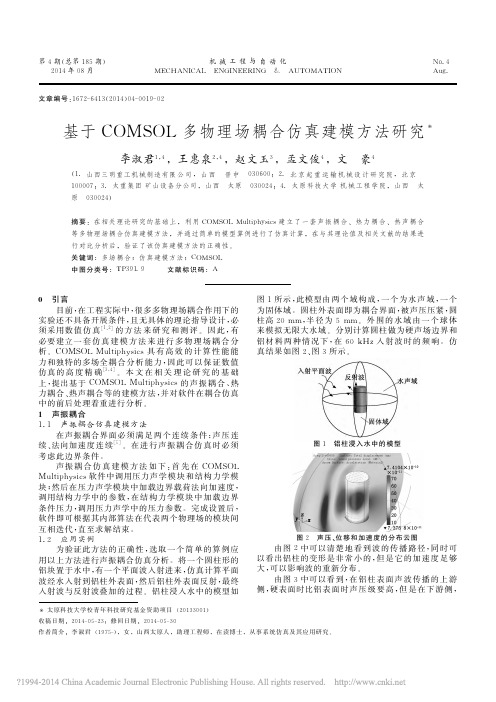
基于COMSOL的母线板多物理场耦合仿真分析

基于COMSOL的母线板多物理场耦合仿真分析程屾;蔡志远【摘要】随着电力工业的快速发展,母线作为汇集、分配和传送电能的装置,广泛应用于各电工领域,但由于其流过电流较大,其温升发热问题不容忽视,该问题涉及到电磁场、温度场、流场及位移场等多物理场的综合应用.为了更好地研究其发热散热问题,采用COMSOL Multiphysics多物理场直接耦合分析软件,基于有限元理论,在考虑设备几何形状和材料物理特性影响的基础上,对母线板进行三维建模,分别在瞬态和稳态情况下对母线板进行电—热—力耦合场分析,电—热—流耦合场分析,研究母线板的温度、电流密度分布规律和由于热膨胀引起的形变大小,最后加入层流,分析在考虑气流冷却效应时母线板的散热情况,并对仿真结果进行研究分析.【期刊名称】《东北电力技术》【年(卷),期】2017(038)007【总页数】5页(P1-4,31)【关键词】母线;多物理场;温升【作者】程屾;蔡志远【作者单位】沈阳工业大学电气工程学院,辽宁沈阳 110870;沈阳工业大学电气工程学院,辽宁沈阳 110870【正文语种】中文【中图分类】U224.2Abstract:With the rapid development of electricity industry, busbars has widely used in various fields of electrical which as a collection, power transmission and distribution device. But due to the flowing current has become larger and larger, the temperature and heat formation can’t be ignored. The problems related to electromagnetic field, temperature field, flow field and field of multi physics field of comprehensive. In order to better study the heat formation and heat dissipation problems.In this paper, based on the finite element theory, by using multidiscipline coupled-field software named COMSOL Multiphysics and considering the geometry and physical properties of the material of equipment,we get the 3D modeling of busbars. Then conduct some coupling field analysis of electric field, thermal field and mechanical field of busbar under transient and steady state separately. As well as some coupling field analysis of electric field, thermal field and flow field. Which can get the distribution law about temperature, current density distribution and the deformation due to thermal expansion of the busbars. Finally, joining laminar flow , the heat dissipation of the busbars has analyzed and the simulation results has analyzed in consideration of the effect of airflow cooling.Key words:busbar; coupled field analysis; thermal expansion随着电气设备容量的不断增大,人们对于电器的性能提出了更高的要求。
comsol多物理场耦合仿真流程
comsol多物理场耦合仿真流程英文回答:COMSOL is a powerful software tool that allows for the simulation of multiphysics phenomena. It enables the coupling of different physical fields, such as heat transfer, fluid flow, and structural mechanics, toaccurately model complex systems and analyze their behavior. The simulation process in COMSOL typically involves several steps, which I will outline below.1. Geometry Definition: The first step is to define the geometry of the system being simulated. This can be done using the built-in CAD tools in COMSOL or by importing a geometry file from an external software. The geometryshould accurately represent the physical system and include all necessary details.2. Physics Setup: Once the geometry is defined, thenext step is to set up the physics of the problem. Thisinvolves selecting the relevant physics modules in COMSOL that correspond to the physical phenomena being simulated. For example, if we are simulating a heat transfer problem, we would select the Heat Transfer module.3. Boundary Conditions and Material Properties: After setting up the physics, we need to define the boundary conditions and material properties. This includes specifying the temperature, pressure, or any other relevant parameters at the boundaries of the system, as well as assigning appropriate material properties to the different regions of the geometry.4. Meshing: Once the physics and boundary conditions are set up, we need to generate a mesh. The mesh divides the geometry into smaller elements, allowing for the numerical solution of the governing equations. The quality of the mesh is important for the accuracy and efficiency of the simulation.5. Solver Settings: After meshing, we need to specify the solver settings. This includes selecting theappropriate solver algorithm, specifying convergence criteria, and setting up any additional solver parameters. The solver is responsible for solving the equations that describe the physical phenomena in the system.6. Running the Simulation: With all the setup steps completed, we can now run the simulation. COMSOL will solve the equations numerically and provide the results for the specified variables of interest. These results can include temperature distributions, velocity profiles, stress distributions, or any other quantities that were defined during the setup.7. Post-processing: Once the simulation is complete, we can analyze and visualize the results using the post-processing tools in COMSOL. This allows us to gain insights into the behavior of the system and evaluate its performance. We can create plots, animations, or export the results for further analysis.In summary, the simulation process in COMSOL involves defining the geometry, setting up the physics and boundaryconditions, meshing the geometry, specifying solver settings, running the simulation, and post-processing the results. This iterative process allows for the accurate modeling and analysis of multiphysics phenomena.中文回答:COMSOL是一款强大的软件工具,可以用于多物理场的仿真。
一种COMSOL与PHREEQC耦合的土壤地下水污染物迁移转化模拟方法[发明专利]
![一种COMSOL与PHREEQC耦合的土壤地下水污染物迁移转化模拟方法[发明专利]](https://img.taocdn.com/s3/m/0e776c7468eae009581b6bd97f1922791688befe.png)
(19)中华人民共和国国家知识产权局(12)发明专利申请(10)申请公布号 (43)申请公布日 (21)申请号 202111429422.7(22)申请日 2021.11.29(71)申请人 上海交通大学地址 201100 上海市闵行区东川路800号(72)发明人 魏亚强 曹心德 赵玲 续晓云 (74)专利代理机构 北京细软智谷知识产权代理有限责任公司 11471代理人 涂凤琴(51)Int.Cl.G06F 30/28(2020.01)G16C 10/00(2019.01)G16C 20/10(2019.01)G06F 113/08(2020.01)G06F 119/14(2020.01)(54)发明名称一种COMSOL与PHREEQC耦合的土壤地下水污染物迁移转化模拟方法(57)摘要本发明属于环境模拟技术领域,具体涉及一种COMSOL与PHREEQC耦合的土壤地下水污染物迁移转化模拟方法,通过获取COMSOL模型的待输入参数数据以及指定时间步长;将所述待输入参数数据以及指定时间步长输入至预构建的COMSOL 模型,计算得到所述待输入参数数据对应的组分的浓度结果;基于Python库PhreeqPy计算所述待输入参数数据对应的组分的浓度结果,将所述待输入参数数据对应的组分的浓度结果输入至PHREEQC中,并进行地球化学反应过程计算,得到下一时间步长以及地球化学反应计算结果;整理重建所述地球化学反应计算结果,并将所述地球化学反应计算结果导入预构建的COMSOL模型中;直至按照所有时间步长模拟得到土壤地下水污染物迁移转化模型。
实现了多物理场和地球化学场的高效模拟。
权利要求书2页 说明书9页 附图4页CN 114201931 A 2022.03.18C N 114201931A1.一种COMSOL与PHREEQC耦合的土壤地下水污染物迁移转化模拟方法,其特征在于,包括:步骤S1、获取COMSOL模型的待输入参数数据以及指定时间步长,所述输入的参数数据与所述指定时间步步长一一对应;步骤S2、将所述待输入参数数据以及指定时间步长输入至预构建的COMSOL模型,计算得到所述待输入参数数据对应的组分的浓度结果;步骤S3、基于Python库PhreeqPy计算所述待输入参数数据对应的组分的浓度结果,将所述待输入参数数据对应的组分的浓度结果输入至PHREEQC中,并进行地球化学反应过程计算,得到下一时间步长以及地球化学反应计算结果;步骤S4、整理重建所述地球化学反应计算结果,并将所述地球化学反应计算结果导入预构建的COMSOL模型中;步骤S5、重复步骤S2‑步骤S4,直至按照所有时间步长模拟得到土壤地下水污染物迁移转化模型。
多物理场耦合分析软件COMSOLMultiphy
多物理场耦合分析软件COMSOLMultiphyCOMSOL Multiphysics AC/DC Module视频教学--2D旋转电机(二)点击下载这个例子是旋转电机模型的扩展,机械运动利用常微分方程描述,计算了电磁力的力矩.此外他利用对称性把模型尺寸降低到原来的八分之一.COMSOL Multiphysics AC/DC Module视频教学--2D旋转电机(一)点击下载这个例子是旋转电机模型的扩展,机械运动利用常微分方程描述,计算了电磁力的力矩.此外他利用对称性把模型尺寸降低到原来的八分之一.COMSOL Multiphysics视频教学--Modelling With Finite Element Methodes第十四章的实例动画和.mph文件点击下载第十四章直流微装置的磁流体动力学数值模拟磁流体动力学理论(MHD)研究电磁场中导电流体的交互作用。
它在很多领域,包括热核反应、太阳和太空等离子体、火箭引擎中都有着非常重要的作用。
目前对MHD的研究兴趣越来越集中在芯片实验中的微尺度流动控制应用上。
驱动MHD微尺度泵的Lorentz力,在方向和大小上取决于施加的磁场B和电场E矢量。
这种泵的主要特性就是可以控制局部流体流动,不需要力学设备就可以精确控制流体在微尺度流道网络中按照预定路径流动。
这种借助Lorentz力的局部流体控制方法使得流体控制变得十分灵活,例如流体可以双向流动、累积、减速甚至回退。
与电动泵使用高的轴线电压相比,MHD微型泵使用低的横向电场。
低的发热量使其可以用于驱动对高温和电压敏感的生物流动过程。
简单的电子设备就可以顺序控制复杂微流动中的各个独立微型泵。
流动速度通过电磁场的强度来控制。
似乎到目前为止仍没有关于MHD微型泵模拟的发表文章。
下面我们将给出一些基于Galerkin有限元法的微型泵模拟结果,模拟过程在商业软件COMSOL Multiphysics 3.2中实现。
数值求解采用压力修正算法--SIMPLE,它首先假设一个压力场,然后通过求解不可压缩流动的Navier-Stokes方程得到速度场。
COMSOL在电解槽中的多物理场耦合研究

COMSOL在电解槽中的多物理场耦合研究电解槽是一种常见的电化学设备,用于电解金属或电解液体中的化学物质。
在电解槽中,电流通过电解质溶液,导致物质的电解反应和转移。
COMSOL Multiphysics能够模拟电解槽中的电流分布、电位分布、气泡生成和流体流动等多种物理过程,实现多物理场的耦合研究。
首先,COMSOL可以模拟电解槽中的电流分布。
通过设定电解槽的几何形状、电极位置和电流密度等参数,COMSOL可以计算出电流在电解质溶液中的分布状况。
这对于电解槽的设计和优化非常重要。
例如,在铝电解工业中,通过优化电极的形状和位置,可以实现电流的均匀分布,提高电解效率和产能。
其次,COMSOL可以模拟电解槽中的电位分布。
通过设定电极的电位、电解质的电导率和电极表面的反应速率等参数,COMSOL可以计算出电解质溶液中的电位分布情况。
这对于了解电解过程中的电极势、浓差极化和电解液中的电位梯度非常重要。
通过优化电位分布,可以减少电极势的损失,提高电解效率。
此外,COMSOL还可以模拟电解槽中的气泡生成和流体流动。
通过设定气体生成速率、气体的溶解度和流体的速度场等参数,COMSOL可以计算出气泡在电解质溶液中的生成和运动情况,进而影响流体流动。
这对于了解电解槽的气泡运动、气体传送和搅拌效果非常重要。
通过优化气泡的生成和流体的流动,可以提高电解槽的传质效率和混合效果。
最后,COMSOL还可以实现多物理场的耦合模拟。
在电解槽中,电流分布、电位分布、气泡生成和流体流动等多个物理过程相互耦合,相互影响。
通过将这些物理过程耦合起来,COMSOL可以模拟电解槽中的整体效应,对优化电解槽的设计和操作提供指导。
综上所述,COMSOL Multiphysics在电解槽中的多物理场耦合研究方面具有广泛的应用。
通过模拟电流分布、电位分布、气泡生成和流体流动等多个物理过程,可以优化电解槽的设计和操作,提高电解效率和产能。
这将对电解工业的发展和节能减排具有重要意义。
COMSOL在微纳光学领域中的应用

Simulating inspires innovation
COMSOL Multiphysics
基于偏微分方程或常微分方程通过 有限元算法实现多场耦合
仿 真 智 领 创 新
Simulating inspires innovation
仿 真 智 领 创 新
Simulating inspires innovation
Matlab PDE Toolbox 1.0 Femlab 1.0 ~ Femlab 3.1(2003年,v3.0具备独立求解器) COMSOL Multiphysics 3.2a (2005年) COMSOL Multiphysics 3.5a COMSOL Multiphysics v4.2a COMSOL Multiphysics 4.3a(现在)
仿 真 智 领 创 新
Simulating inspires innovation
• 选择物理场 -告诉软件分析问题中包含哪些物理现象 • CAD绘图
-软件自带CAD绘图、导入CAD模型
建 模 流 程
• 指定分析条件 -指定材料、输入、输出选项 -指定边界条件 • 网格 -结构化或非结构化网格 • 求解
仿 真 智 领 创 新
Simulating inspires innovation
COMSOL Multiphysics
模块简介
喷气发动机涡轮叶片温度场和应力分布
仿 真 智 领 创 新
Simulating inspires innovation
AC/DC模块
AC/DC模块的功能涵盖了静电场、静磁场、 直流交流电磁,以及与其它物理场的无限制耦合。 • 电容器 • 电感器
COMSOL Multiphysics在医疗药物中的应用
COMSOL Multiphysics在医疗药物中的应用“通过对新产品进行设计和改进,计算机建模已经证明了它的价值。
”这是John Kalafut,一位MEDRAD研发部门(Indianola,Pennsylvania)的首席研究学者的经验之谈,他指出“COMSOL Multiphysics在我的整个职业生涯中陪伴着我,最初是在MEDRAD公司的系统工程方面,现在则是在R&D方面,甚至是用在那些多年后才能商业化量产的产品上”。
Kalafut作为一个医学工程师的经验显示了在很多时候我们都需要解决多物理场耦合模型的问题。
MEDRAD,一个每年有5亿美元销售额的成像诊断和治疗的医学设备生产商、销售商和服务提供商,它的业务主要集中在三个领域:心脑血管诊断,磁共振成像,X线断层摄影术。
公司在世界范围内有1700名员工,来自全世界的医师每年使用该公司的两千万个医疗程序。
公司的核心竞争力之一就是血管内流体输送,比如,如何供应精确的药剂量或者造影剂的量。
公司的研发部门为了保持公司每年15%的成长速度负责研究新型的技术,投资商业项目和医学应用。
公司的5名工程师利用COMSOL软件解决了大量的难题。
Kalafut说,“COMSOL Multiphysics是一个自然地选择,它可以给我们在一些新概念的研究上提供支持,对于所有的生物医学工程师而言这是帮助我们研究的相当有利的一个工具,它的完全的多场耦合仿真能力意味着我们几乎可以处理任何的多场耦合问题。
COMSOL Multiphysics让我们花费不多的钱来对复杂的耦合现象有一个快速的认识和研究。
”从建模的角度来看,很多公司的研究涉及到如何用最有效,最安全的方式去传输那些帮助诊断的流体到病人的身体中去。
在类似的研究中流体动力学发挥着一个重要的作用,这些模型包括热传导、静电学、化学工程、电磁学和其他物理方面的模型。
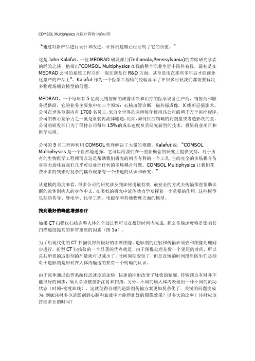
找到最好的峰值增强治疗如果CT扫描仪扫描完整人体的全部过程可以在很短时间内完成,那么传输速度将是影响其扫描速度提高的非常重要的因素(图1a)。
基于COMSOL的电磁搅拌器的多物理场耦合有限元建模研究
基于COMSOL的电磁搅拌器的多物理场耦合有限元建模研究发表时间:2019-05-27T10:52:49.297Z 来源:《电力设备》2018年第35期作者:公伟凯张海燕王友情周旋[导读] 摘要:电磁搅拌过程是一个多物理场之间的强耦合作用过程,研究电磁搅拌器主要采用数值分析方法,电磁搅拌器多物理场耦合模型的建立是准确研究电磁搅拌原理和液面波动的基础和保障。
(上海电机学院电气学院上海 201306)摘要:电磁搅拌过程是一个多物理场之间的强耦合作用过程,研究电磁搅拌器主要采用数值分析方法,电磁搅拌器多物理场耦合模型的建立是准确研究电磁搅拌原理和液面波动的基础和保障。
首先对结晶器电磁搅拌器的电磁场数学模型和湍流场数学模型进行了推导,并建立多物理场耦合关系,然后基于COMSOL软件详细研究了电磁搅拌器多物理场耦合模型的建模方法,建立了COMSOL有限元仿真模型,并给出详细建模参数和步骤;最后,通过分析仿真结果,研究了电磁搅拌器电磁场和钢液转速分布规律。
关键词:结晶器电磁搅拌器;多物理场耦合;电磁力;COMSOL有限元仿真模型;0 引言由于电磁搅拌技术高能量密度、高清洁度、高可靠度、高可控度和高自动化等优越性,在连铸冶金行业中被广泛应用[1]。
由于实际操作环境高温、危险等问题,有限元仿真模拟是目前研究电磁搅拌器的有效手段。
电磁搅拌有限元建模是一个多物理场强双向耦合问题,模型收敛困难,通常会将模型解耦。
文献[2]采用CFX软件对大方坯结晶器内钢水流动过程进行理论计算和分析,评估浸入式水口结构对结晶器内流场、自由液面波动的影响,但未涉及电磁搅拌。
文献[3]同样借助ANSYS软件计算出电磁场分布,再利用自编程将磁力线线性插值到FLUENT中实现耦合。
文献[4]介绍了电磁搅拌器ANSYS的建模过程,但并没有涉及与流场的耦合。
文献[5-6]借助COMSOL软件对电磁搅拌器进行了仿真实验,但并未明确给出耦合方式和建模步骤。
COMSOL软件在流体结构传热等多物理场耦合领域的应用

COMSOL软件在流体结构传热等多物理场耦合领域的应用COMSOL软件是一款强大的多物理场耦合仿真软件,广泛应用于流体、结构、传热等领域。
其灵活的模型构建和求解技术使其成为工程师和科学家解决复杂的多物理问题的首选工具。
以下将详细介绍COMSOL在流体、结构和传热领域的应用。
在流体领域,COMSOL可用于流体流动、传质、多相流和空气动力学等问题的建模和仿真。
例如,在流体流动领域,COMSOL可以用于模拟和分析各种流动情况,如湍流、边界层、旋转流动等。
通过使用不同的物理模型和边界条件,可以模拟各种复杂的流体行为,如湍流的涡街和流过物体的气流。
COMSOL还能够进行流体和结构耦合仿真,模拟流体对结构的影响,如振动和压力。
在结构领域,COMSOL可用于机械振动、固体力学和结构动力学等问题的建模和仿真。
例如,在机械振动分析中,COMSOL可以模拟机械系统的自由振动和强迫振动,并分析其频率响应和模态形状。
在固体力学领域,COMSOL可以用于模拟和分析各种材料的应力和应变分布,以及结构的变形和失稳行为。
COMSOL还可以进行结构和流体耦合仿真,模拟流体对结构的振动和压力的影响。
在传热领域,COMSOL可以用于模拟和分析各种传热问题,如热传导、对流传热、辐射传热和相变传热等。
例如,在热传导分析中,COMSOL可以用于模拟材料的温度分布和传热速率,以及热源对材料的影响。
在对流传热分析中,COMSOL可以模拟流体流动对传热的影响,例如冷却系统中的换热器和散热器。
COMSOL还可以模拟辐射传热,如太阳辐射和热辐射传热。
此外,COMSOL还可以进行传热和结构耦合仿真,模拟传热对结构的变形和失稳的影响。
除了以上介绍的领域,COMSOL还广泛应用于其他领域,如化学工程、电磁场、声学和生物医学等。
通过灵活的模型构建和求解技术,COMSOL可以与其他领域的模型进行耦合,实现多物理场的综合仿真。
总之,COMSOL软件在流体、结构、传热等多物理场耦合领域具有广泛的应用。
COMSOL工程应用系列手册-多物理场仿真在电子设备热管理中的应用说明书

COMSOL APPLICATION NOTES | 1COMSOL 工程应用系列手册多物理场仿真在电子设备热管理中的应用多物理场仿真在电子设备热管理中的应用目 录简介 3工程目标 4电子设备的热管理 4传热的应用领域 4传热机理 5数值仿真 6电子设计中的数值仿真 6传热建模的物理场接口 7单物理场接口 8多物理场接口 9扩展接口 10建模案例 10平板上方的非等温湍流 10圆管中的非等温层流 11一种热光型硅光子开关的优化 11平板热管的传热与流体动力学 12大型强子对撞机中的超导磁体 12植入式医疗设备的温度适应性 13仿真 App 案例 14使用仿真 App 进行传热与流体动力学教学 14使用仿真 App 模拟定制化电容器 15使用仿真 App 比较石墨箔传热性能 16结语 17参考文献 18更多资源 19© 版权所有 2019 COMSOL。
《多物理场仿真在电子设备热管理中的应用》由 COMSOL,公司及其关联公司发布。
COMSOL、COMSOL 徽标、COMSOL Multiphysics、COMSOL Desktop、COMSOL Server 和 LiveLink 均为 COMSOL AB 公司的注册商标。
所有其他商标均为其各自所有者的财产, COMSOL AB 公司及其子公司和产品与上述非 COMSOL 商标所有者无关,亦不由其担保、赞助或支持。
相关商标所有者的列表请参见 /trademarks。
2 | COMSOL 工程应用系列手册COMSOL 工程应用系列手册 | 3简介简 介通常,在设计电子设备时,需要充分考虑热管理因素。
随着设备性能的提升和市场竞争的加剧,为了实现可靠性更高、能耗和成本更低、安全性更强以及用户体验更好的设计目标,越来越多的研究人员开始使用数值仿真技术进行设计工作。
本手册介绍的仿真案例涉及多种系统,这些系统各不相同,但均有电流存在。
在这些案例以及大多数工程应用案例中,对系统中引起温度变化的传热机制和因素进行研究,可以帮助工程师更好地理解设计对产品性能产生的影响。
Comsol软件介绍
我不是做广告的啊COMSOL介绍COMSOL Multiphysics多物理关注前沿科技,解决多场直接耦合难题——COMSOL Multiphysics助您登上科学的巅峰COMSOL Multiphysics是一款大型的高级数值仿真软件。
广泛应用于各个领域的科学研究以及工程计算,被当今世界科学家称为“第一款真正的任意多物理场直接耦合分析软件”。
模拟科学和工程领域的各种物理过程,COMSOL Multiphysics以高效的计算性能和杰出的多场双向直接耦合分析能力实现了高度精确的数值仿真。
COMSOL公司于1986 年在瑞典成立,目前已在全球多个国家和地区成立分公司及办事机构。
COMSOL Multiphysics起源于MATLAB的Toolbox,最初命名为Toolbox 1.0。
后来改名为Femlab 1.0(FEM为有限元,LAB是取自于Matlab),这个名字也一直沿用到Femlab 3.1。
从2003年3.2a版本开始,正式命名为COMSOL Multiphysics。
COMSOL Multiphysics以其独特的软件设计理念,成功地实现了任意多物理场、直接、双向实时耦合,在全球领先的数值仿真领域里得到广泛的应用。
在全球各著名高校,COMSOL Multiphysic已经成为教授有限元方法以及多物理场耦合分析的标准工具,在全球500强企业中,COMSOL Multiphysic被视作提升核心竞争力,增强创新能力,加速研发的重要工具。
2006年COMSOL Multiphysics再次被NASA技术杂志选为"本年度最佳上榜产品",NASA 技术杂志主编点评到,"当选为NASA科学家所选出的年度最佳CAE产品的优胜者,表明COMSOL Multiphysics是对工程领域最有价值和意义的产品。
"COMSOL Multiphysics显著特点求解多场问题= 求解方程组,用户只需选择或者自定义不同专业的偏微分方程进行任意组合便可轻松实现多物理场的直接耦合分析。
岩土工程中水热力三场耦合的计算模型及数值模拟方案

计算结果
温度场变化
温度场变化曲线
路基中心点,温度变化曲线
应变曲线
应变曲线
应变曲线
路基顶面中心点应变曲线
小结
• 由于没有考虑相变的影响,路基考虑为弹性本构。 • 所以,结构呈现很好的线性曲线。但,不考虑相变的影响, • 土体的温度热膨胀应变不大。 • 下一步工作 • 在模型中加入水分场并加入相变变化。 • 把模型更加细化,路基土层分层建立,设置不同材料参数。 • 结合前期观察的冻土数据进行比较。 • 模型建立完成后,也可以考虑在模型上加载汽车动荷载。
其中t的单位为旬,即10天。
温度拟合值
拟合温度值
拟合温度曲线
温度场边界条件
• 单位的转化。COMSOL单位是S,需要对单位进行转换, 并改写成COMSOL格式。
应力场模型
• 本构关系选取弹性本构。
边界条件
三边固定边界、顶部自由边界。
初值:考虑重力影响。
求解
• 计算步长 • 由于已旬为单位。 • 总计计算一年,总计36旬 • 每一旬输出一个结果。 • 计算了2年
[a]:热膨胀系数
•
T:温度
• 根据后面的计算土体在未冻结的情况下温度变化的膨胀很 小,约有零点几毫米。
• 所以,主要考虑的还是相变引起的热膨胀
介绍几个模型
• 在多孔介质中,水热耦合作用下,土中水分的迁移和温度 场的分布模型。
• 选取矩形二维土箱
温度引起的渗流场流动
流速场
温度场
水分迁移
模型建立
冰水相变模型
选取一个冰柱
伴随相变的温度 变化曲线
会进一步把相变融入到 模型中
基坑开挖
COMSOL优劣简介
• 优势 • COMSOL的特点就是多场耦合的计算。 • 核心是解偏微分方程。 • 计算速度快
COMSOL软件在流体、结构、传热等多物理场耦合领域的应用.docx

Subsurface Flow Module基于地下水流动分析地球物理现象2 000 years在建的核废料储存库,用于在接下来的10万年内储存乏燃料棒。
该模型模拟的情形是: 燃料束套筒发生破裂,导致核废料通过周闌的岩石裂隙发生渗漏,并回充到上方的隧道中。
饱和与变饱和渗流地卜水流动模块面向需要仿真地卞或其他多孔介质中的流体流动的工程师和科学家们,并且还可以将这种流动过程与其他现象建立联系,例如多孔弹性、传热、化学反应和电磁场等。
它可以用于模拟地下水流动、废料与污染物在土壤中的扩散、油与气体的流动,以及由于地下水开采而引发的土地沉陷等现彖。
地下水流动模块可以模拟管道流、饱和与变饱和多孔介质或裂隙中的地下水,并可与传质、传热、地球化学反应和多孔弹性等模型相耦合。
许多不同的行业需要面对岩土物理和水力领域的挑战。
民事、采矿、石油、农业、化工、核能和坏境工程等领域的工程师经常需要考虑这些现象,因为他们从事的行业会直接或间接(通过环境因素)影响我们生存的地球环境。
地下水渗流影响许多地球物理属性地卜•水流动模块内包含了许多专用的接11,用于模拟地卞环境中的流动及其他现彖。
作为物理接II,它们可以与地下水流动模块内的其他任意物理接11组合并直接耦合,或与COMSOL模块套件中任何其他模块的物理接II组合并直接耦合。
例如,地下水流动模块的多孔弹性模型与左土力学模块中的描述土壤和岩石的非线性固体力学模型相耦合。
融合地球化学反应速率和动力场COMSOL使您可以在地卞水流动模块物理接I I中的编辑区域内灵活地输入任意公式,这对于在质量传递接II中定义地球化学反应速率和动力场非常有用。
但是,将这些物理接II 与化学反应工程模块耦合将意味着,您可以通过该模块易用的物理接II定义化学反应,模拟多个多物质反应。
对于模拟核废料数T•年间在其储存库中的扩散及多步反应过程,这两种模块的组合会很有用。
更多图片Time =86400 Surfge■: Effecth/e saturation (1) Contour: Pressure heotf (m> 0O1 -0.2 0304 0506 0.708 09•1•1.14.2•1.3095690-85.0.80-7 &0.7▼ 0.6843地下水流动的仿真物理接口地下水流动模块用于仿真多孔介质流动及其相关过程:多孔介质流动地卜水流动模块的核心功能是模拟变饱和与完全饱和多孔介质中的流动。
COMSOL_Multiphysics在岩土工程中的应用

COMSOL Multiphysics在岩土工程中的应用摘要:目前,COMSOL Multiphysics作为全球第一款真正的多物理场耦合分析软件,由于其具有多场问题全耦合分析的强大功能,能够帮助科研人员得到更精确地模拟结果,被广泛适用于岩土工程研究的各个领域。
本文就COMSOL Multiphysics在岩土工程中采矿工程中的岩土工程问题、氯盐对混凝土耐久性影响的问题、基桩动测问题方面的应用作出相应简单的介绍。
阐述COMSOL Multiphysics软件在该领域的强大功能和适用性,说明COMSOL Multiphysics 在岩土工程中的应用。
1.多物理场耦合数值模拟软件系统(COMSOL Multiphysics)的介绍多物理场耦合数值模拟软件系统(COMSOL Multiphysics)是一个专业有限元数值分析软件包,是专为描述和模拟各种物理现象而开发的基于偏微分方程的多物理场模型仿真计算的有限元分析软件包。
COMSOL Multiphysics软件系统包括结构力学、化学、电磁学、地球科学、微机电、声学等模块。
在使用COMSOL Multiphysics软件的过程中,用户可以自己建立普通的偏微分方程形式,也可以使用COMSOLMultiphysics提供的特定的物理应用模型。
这些特定的物理应用模型包括预先设定好的模块和在一些特殊应用领域内已经通过微分方程和变量建立起来的用户界面。
通过COMSOL Multiphysics的多物理场功能,用户可以选择不同的模块,同时模拟任意物理场组合进行耦合分析。
为了便于比较, 在COMSOL Multiphysics结构力学模块中,用户可以完全利用COMSOL Multiphysics中无限制多物理场和基于偏微分方程的表达式进行分析,因此可以随意地将结构力学分析与其它物理现象如电磁场、流场和热传导等耦合起来进行分析。
SOL Multiphysics在采矿工程中的岩土工程问题中的应用伴随采矿工程中的岩土工程问题常常是复杂的多物理场耦合问题,其基本问题是岩体或土体的稳定、变形和渗流问题、煤层甲烷运移问题。
COMSOL_Multiphysics介绍

COMSOL Multiphysics 允许用户通过参数控制的方式灵活的调整模型的几何尺寸。这在进 行设计的优化分析时尤其有用,能够帮助用户节省大量的时间,只需要调整相应参数的值并 重新计算就可以完成一个新的模型的仿真分析。
¾ 开放性 对用户透明,可任意修改现有模型 支持建立自己的模型/方程
¾ 灵活性 与 MATLAB 无缝连接,提供强大的二次开发功能 JAVA 编程:基于 JAVA 标准的 API,构建自己的有限元软件
产品线示意图
中仿科技公司 CnTech Co., Ltd
全国统一客户服务热线:400 888 5100 网址: 邮箱:info@ -5-
中仿科技公司 CnTech Co., Ltd
系数型 PDE 应用模式的一般方程形式: ∇ ⋅ (− c∇u − αu + γ ) + au + β ⋅ ∇u = f
采用填空的形式输入方程:c = 1,f = 1,其余系数均设为 0,如下图:
B. 使用预置应用模式建模 除了强大而开放的 PDE 数值计算功能,COMSOL Multiphysics 还根据常见的应用领域,
跨学科研究和多物理分析为科研创新带来了新契机,而构建于简化与单物理分析的思维 基础上的基于观察与实验的研究方 法却面临越来越大的挑战。今天,人 们已经知道超级计算机也是衡量一 个国家核心竞争力的重要指标。不论 是科学研究还是产品开发,实验研究 与仿真技术的结合已经是大势所趋, 而且数值仿真正在发挥越来越重要 的作用。
中仿科技公司 CnTech Co., Ltd
COMSOL Multiphysics
comsol仿真实验报告

comsol仿真实验报告一、实验目的本次实验旨在通过使用 COMSOL Multiphysics 软件对特定的物理现象或工程问题进行仿真分析,深入理解相关理论知识,并获取直观、准确的结果,为实际应用提供有效的参考和指导。
二、实验原理COMSOL Multiphysics 是一款基于有限元方法的多物理场仿真软件,它能够将多个物理场(如电场、磁场、热场、流体场等)耦合在一个模型中进行求解。
其基本原理是将连续的求解区域离散化为有限个单元,通过对每个单元上的偏微分方程进行近似求解,最终得到整个区域的数值解。
在本次实验中,我们所涉及的物理场及相关方程如下:(一)热传递热传递主要有三种方式:热传导、热对流和热辐射。
热传导遵循傅里叶定律:$q =k\nabla T$,其中$q$ 为热流密度,$k$ 为热导率,$\nabla T$ 为温度梯度。
热对流通过牛顿冷却定律描述:$q = h(T T_{amb})$,其中$h$ 为对流换热系数,$T$ 为物体表面温度,$T_{amb}$为环境温度。
(二)流体流动对于不可压缩流体,其运动遵循纳维斯托克斯方程:$\rho(\frac{\partial \vec{u}}{\partial t} +(\vec{u}\cdot\nabla)\vec{u})=\nabla p +\mu\nabla^2\vec{u} +\vec{f}$其中$\rho$ 为流体密度,$\vec{u}$为流体速度,$p$ 为压力,$\mu$ 为动力粘度,$\vec{f}$为体积力。
(三)电磁场麦克斯韦方程组是描述电磁场的基本方程:$\nabla\cdot\vec{D} =\rho$$\nabla\cdot\vec{B} = 0$$\nabla\times\vec{E} =\frac{\partial \vec{B}}{\partial t}$$\nabla\times\vec{H} =\vec{J} +\frac{\partial \vec{D}}{\partial t}$其中$\vec{D}$为电位移矢量,$\vec{B}$为磁感应强度,$\vec{E}$为电场强度,$\vec{H}$为磁场强度,$\rho$ 为电荷密度,$\vec{J}$为电流密度。
COMSOL多物理场耦合仿真建模方法
( 英文摘要转第 2 3 页)
1 4 年第 4 期 机 械 工 程 与 自 动 化 2 0
·2 3·
3 结束语 本文基于 M d e l i c a 语 言 在 MW o r k s平 台 上 实 现 o 了对房间空调器主要 部 件 的 建 模 , 并建立了制冷剂的 热力性质及热物理性质计算函数库 。 在此基础上建立 对冷凝器ห้องสมุดไป่ตู้热量 与 了空调制冷系统的 M d e l i c a模型 , o
3 热声耦合 1 热 声耦合仿真 建模 方 法 3. 7] 实 际 上 就 是 热 与 声 的 相 互 转 化。 热声耦合效应 [ 热量分布会引起传声 介 质 的 密 度 变 化 , 进而影响声场 的分布 , 同时由于热场中各处声压不同 , 热场分布也会 因此而产生变化 。 热声 耦 合 仿 真 建 模 方 法 如 下: 首先在 C O L OMS M u l t i h s i c s软 件 中 调 用 压 力 声 学 模 块 和 传 热 模 块 , p y 在压力声学模块中调 用 传 热 学 中 的 温 度 分 布 参 数 , 在 传热模块中添加声压 边 界 条 件 ; 接下来软件会在代表 热场和声场的两个模 块 之 间 来 回 迭 代 , 每次运算都要 , 调用前一次的结果 进 而 仿 真 出 热 和 声 之 间 的 相 互 影 响。 2 应 用实例 3. 为验证此方法的正确性同样选取了简单的模型来 进行热声耦合仿真分析 。 建立一个正方形的空气域模 型, 分两种情况进行了模拟 , 第一种情况下温度场分布 达 均匀 , 第二种情况下 左 侧 温 度 比 右 侧 温 度 高 6 0 ℃, 到稳态后温度沿 x 轴 为 线 性 分 布 。 两 种 情 况 下 , 在左 , 。 大小为 2P 侧加一个入射平面波 , 其频率为 5 0H z a 0 图 6 为热场分布对声场分布的影响 。 由图 6 中可以看 出, 有温度场分布情况下声场分布更密集一些 。 根据理论我们可 以 知 道 , 温度高的地方气体的密 度会下降 , 在此处的声速就会下降 , 在频率不变的情况 下, 其波长就会变短 , 其声场分布就会变得密集 。 仿真结果与理论 推 导 一 致 , 说明该仿真建模方法 。 的正确性
COMSOL使用技巧_V1.0_2013-02

COMSOL 使用技巧中仿科技公司CnTech Co.,Ltd目录一、1.11.21.31.41.51.6二、2.12.22.32.4三、3.13.23.33.43.5四、4.14.24.34.44.5五、5.15.25.3六、6.16.26.36.46.5七、几何建模................................................................................................................................. - 1 -组合体和装配体................................................................................................................. - 1 -隐藏部分几何..................................................................................................................... - 2 -工作面................................................................................................................................. - 3 -修整导入的几何结构......................................................................................................... - 4 -端盖面............................................................................................................................... - 11 -虚拟几何........................................................................................................................... - 12 -网格剖分............................................................................................................................... - 14 -交互式网格剖分............................................................................................................... - 14 -角细化............................................................................................................................... - 16 -自适应网格....................................................................................................................... - 16 -自动重新剖分网格........................................................................................................... - 18 -模型设定............................................................................................................................... - 19 -循序渐进地建模............................................................................................................... - 19 -开启物理符号................................................................................................................... - 19 -利用装配体....................................................................................................................... - 21 -调整方程形式................................................................................................................... - 22 -修改底层方程................................................................................................................... - 23 -求解器设定........................................................................................................................... - 25 -调整非线性求解器........................................................................................................... - 25 -确定瞬态求解的步长....................................................................................................... - 26 -停止条件........................................................................................................................... - 27 -边求解边绘图................................................................................................................... - 28 -绘制探针图....................................................................................................................... - 29 -弱约束的应用技巧............................................................................................................... - 31 -一个边界上多个约束....................................................................................................... - 31 -约束总量不变................................................................................................................... - 32 -自定义本构方程............................................................................................................... - 34 -后处理技巧........................................................................................................................... - 36 -组合图形........................................................................................................................... - 36 -显示内部结果................................................................................................................... - 37 -绘制变形图....................................................................................................................... - 38 -数据集组合....................................................................................................................... - 39 -导出数据........................................................................................................................... - 39 -函数使用技巧....................................................................................................................... - 43 -7.17.27.37.4八、8.18.2九、9.19.2十、10.110.210.310.4十一、11.111.211.311.411.511.6随机函数........................................................................................................................... - 43 -周期性函数....................................................................................................................... - 44 -高程函数........................................................................................................................... - 45 -内插函数........................................................................................................................... - 46 -耦合变量的使用技巧........................................................................................................... - 48 -积分耦合变量................................................................................................................... - 48 -拉伸耦合变量................................................................................................................... - 49 -ODE 的使用技巧................................................................................................................... - 50 -模拟不可逆形态变化....................................................................................................... - 50 -反向工程约束................................................................................................................... - 51 -MATLAB 实时链接................................................................................................................ - 52 -同时打开两种程序GUI................................................................................................. - 52 -在COMSOL 中使用MATLAB 脚本................................................................................ - 52 -在MATLAB 中编写GUI ................................................................................................. - 53 -常用脚本指令................................................................................................................ - 54 -其他................................................................................................................................... - 56 -局部坐标系.................................................................................................................... - 56 -应力集中问题................................................................................................................ - 56 -灵活应用案例库............................................................................................................ - 57 -经常看看在线帮助........................................................................................................ - 57 -临时文件........................................................................................................................ - 58 -物理场开发器................................................................................................................ - 59 -一、几何建模COMSOL Multiphysics 提供丰富的工具,供用户在图形化界面中构建自己的几何模型,例如1D 中通过点、线,2D 中可以通过点、线、矩形、圆/椭圆、贝塞尔曲线等,3D 中通过球/椭球、立方体、台、点、线等构建几何结构,另外,通过镜像、复制、移动、比例缩放等工具对几何对象进行高级操作,还可以通过布尔运算方式进行几何结构之间的切割、粘合等操作。
comsol仿真案例

comsol仿真案例Comsol仿真案例。
在工程领域,仿真技术被广泛应用于产品设计、工艺优化、性能预测等方面。
Comsol Multiphysics作为一款多物理场仿真软件,具有强大的建模和求解能力,能够模拟电磁、结构力学、流体力学等多个物理场的耦合效应,为工程师和科研人员提供了强大的工具来解决复杂问题。
本文将以一个实际案例来介绍Comsol Multiphysics的仿真应用。
我们将以磁场传感器的设计为例,展示如何利用Comsol进行多物理场的仿真分析。
首先,我们需要建立磁场传感器的几何模型。
在Comsol中,可以通过几何建模模块来创建传感器的三维几何结构,包括传感元件的形状、尺寸和材料属性等。
在建模过程中,可以直观地观察和调整传感器的几何参数,以满足设计要求。
接下来,我们需要定义磁场传感器的物理特性。
通过Comsol的物理场模块,可以添加磁场、电磁感应等物理场效应,并设置材料的磁性参数、电导率等物理属性。
这些物理特性将直接影响传感器的性能和响应。
然后,我们可以进行多物理场的耦合仿真。
Comsol Multiphysics能够同时求解多个物理场的方程,并考虑它们之间的相互作用。
在磁场传感器的案例中,我们可以将磁场、电磁感应和结构力学等物理场进行耦合,分析传感器在外部磁场作用下的响应和变形情况。
在仿真过程中,可以通过Comsol的后处理模块来可视化仿真结果,包括磁感应强度分布、电流密度分布、应力应变分布等。
这些结果能够直观地展现传感器的工作状态和性能表现,为设计优化和性能预测提供重要参考。
最后,我们可以通过参数化设计和优化算法,对传感器的关键参数进行调整和优化。
Comsol Multiphysics提供了丰富的参数化建模和优化工具,能够快速高效地进行设计方案的评估和优化,以实现传感器性能的最大化。
总的来说,Comsol Multiphysics作为一款多物理场仿真软件,能够为工程师和科研人员提供强大的仿真分析工具,帮助他们解决复杂的工程和科学问题。
- 1、下载文档前请自行甄别文档内容的完整性,平台不提供额外的编辑、内容补充、找答案等附加服务。
- 2、"仅部分预览"的文档,不可在线预览部分如存在完整性等问题,可反馈申请退款(可完整预览的文档不适用该条件!)。
- 3、如文档侵犯您的权益,请联系客服反馈,我们会尽快为您处理(人工客服工作时间:9:00-18:30)。
Inductor in an Amplifier CircuitThis model studies a finite element model of an inductor inserted into an electrical amplifier circuit.IntroductionModern electronic systems are very complex and depend heavily on computer aided design in the development and manufacturing process. Common tools for suchcalculations are based on the SPICE format originally developed at Berkeley University (Ref. 1). The SPICE format consists of a standardized set of models for describing electrical devices—especially semiconductor devices such as transistors, diodes, and thyristors. SPICE also includes a simple, easy-to-read text format for circuit netlists and model parameter specifications. Although the netlist format is essentially the same as it was from the beginning, the set of models and model parameters constantly changes, with new models being added according to the latest achievements in semiconductor device development. When the devices are scaled down, new effects appear that have to be properly modeled. The new models are the result of ongoing research in device modeling.When an engineer is designing a new electronic component, like a capacitor or an inductor, the SPICE parameters for that device are not known. They are eitherextracted from finite element tools such as COMSOL Multiphysics or frommeasurements on a prototype. To speed up the design process it can be convenient to include the finite element model in the SPICE circuit simulation, calculating the device behavior in an actual circuit.This model takes a simple amplifier circuit and exchanges one of its components witha finite element model of an inductor with a magnetic core. COMSOL Multiphysicscalculates the transient behavior of the entire system. Importing a SPICE circuit netlist brings in the circuit elements along with their model parameters and location in the circuit. All elements can be edited in COMSOL Multiphysics, and any pair of nodes can connect to the finite element model.Model DefinitionThe inductor model uses the Magnetic Fields physics of the AC/DC Module, solving for the magnetic potential A:where μ0 is the permeability of vacuum, μr the relative permeability, and σ the electrical conductivity.Because the inductor has a large number of turns it is not efficient to model each turn as a separate wire. Instead the model treats the entire coil as a block with a constant external current density corresponding to the current in each wire. The conductivity in this block is zero to avoid eddy currents, which is motivated by the fact that no currents can flow between the individual wires. The eddy currents within each wire are neglected.C O N N E C T I O N T O A S P I C E C I R C U I TThe electrical circuit is a standard amplifier circuit with one bipolar transistor, biasingresistors, input filter, and output filter (see the figure below).The input is a sine signal of 1 V and 10 kHz. The following listing shows the SPICE netlist for this circuit:* BJT Amplifier circuit.OPTIONS TNOM=27.TEMP 27Vin 1 0 sin(0 1 10kHz)Vcc 4 0 15Rg 1 2 100σA ∂t∂------∇μ01–μr 1–∇A ×()×+J e =Cin 2 3 10uR1 4 3 47kR2 3 0 10kX1 4 5 inductorRE 7 0 1kCout 5 6 10uRl 6 0 10kQ1 5 3 7 BJT.MODEL BJT NPN(Is=15f Ise=15f Isc=0 Bf=260 Br=6.1+ Ikf=.3 Xtb=1.5 Ne=1.3 Nc=2 Rc=1 Rb=10 Eg=1.11+ Cjc=7.5p Mjc=.35 Vjc=.75 Fc=.5 Cje=20p Mje=0.4 Vje=0.75+ Vaf=75 Xtf=3 Xti=3).SUBCKT inductor V_coil I_coil COMSOL: *.ENDS.ENDThe device X1 refers to a subcircuit defined at the end of the file. The subcircuit definition is part of the SPICE standard to define blocks of circuits that can be reused in the main circuit. The special implementation used here defines a subcircuit that really is a COMSOL Multiphysics model, referenced with the optionCOMSOL: <file name>|<physics_interface_name>|*. The asterisk means that COMSOL Multiphysics looks for the first occurrence of the specified parametersV_coil and I_coil in the current model. These parameters are the variables that link the model with the circuits, and must be defined in the model in a certain way. The variable V_coil must give the voltage over the device, defined in the global scope. I_coil must be a global variable used in the model as a current through the device.The model parameters of the transistor do not correspond to a real device, but the numbers are nevertheless chosen to be realistic.The import of the SPICE netlist does not fully support the SPICE format; especially for the semiconductor device models it only supports a limited set of parameters. Supplying unsupported parameters results in those parameters not being used in the circuit model. For example, transit time capacitance and temperature dependence are not supported for the transistor model.Results and DiscussionA first version of this model lets you compute the magnetic flux density distribution from a 1 A current through the inductor, without the circuit connection taken into consideration.Figure 1: Magnetic flux density distribution as the coil is driven by a 1 A current source. Biasing of an amplifier is often a complicated compromise, especially if you only use resistors. Adding an inductor as the collector impedance simplifies the biasing design, because the instantaneous voltage on the collector of the transistor can be higher than the supply voltage, which is not possible with resistors. Amplifiers using inductors can be quite narrow banded.Before starting the transient simulation, proper initial conditions have to be calculated. For this model it is sufficient to ramp the supply voltage to 15 V with the nonlinear parametric solver. After the ramp, the DC bias conditions have been calculatedproperly, and you can use this solution as initial condition for the transient simulation.Using a global variables plot, you can easily plot input signal, output signal, and inductor voltage in the same figure.Figure 2: Input signal (cir.VIN_v), output signal (cir.RL_v), and inductor voltage(cir.X1_v) as functions of time.The output signal is about 1.5 times the input signal in amplitude.Reference1. The SPICE home page, /Classes/IcBook/SPICE.Model Library path: ACDC_Module/Inductive_Devices_and_Coils/inductor_in_circuitModeling InstructionsFrom the File menu, choose New.N E W1In the New window, click Model Wizard.M O D E L W I Z A R D1In the Model Wizard window, click 2D Axisymmetric.2In the Select physics tree, select AC/DC>Magnetic Fields (mf).3Click Add.4Click Study.5In the Select study tree, select Preset Studies>Stationary.6Click Done.G E O M E T R Y11In the Model Builder window, under Component 1 (comp1) click Geometry 1.2In the Settings window for Geometry, locate the Units section.3From the Length unit list, choose mm.Circle 1 (c1)1On the Geometry toolbar, click Primitives and choose Circle.2In the Settings window for Circle, locate the Size and Shape section.3In the Radius text field, type 30.4Click the Build Selected button.Rectangle 1 (r1)1On the Geometry toolbar, click Primitives and choose Rectangle.2In the Settings window for Rectangle, locate the Size section.3In the Width text field, type 40.4In the Height text field, type 80.5Locate the Position section. In the z text field, type -40.6Click the Build Selected button.Intersection 1 (int1)1On the Geometry toolbar, click Booleans and Partitions and choose Intersection. 2Select both the circle and the rectangle.3Click the Build Selected button.4Click the Zoom Extents button on the Graphics toolbar.Rectangle 2 (r2)1On the Geometry toolbar, click Primitives and choose Rectangle.2In the Settings window for Rectangle, locate the Size section.3In the Width text field, type 5.4In the Height text field, type 20.5Locate the Position section. In the z text field, type -10.6Click the Build Selected button.Rectangle 3 (r3)1On the Geometry toolbar, click Primitives and choose Rectangle.2In the Settings window for Rectangle, locate the Size section.3In the Width text field, type 3.4In the Height text field, type 20.5Locate the Position section. In the r text field, type 7.5.6In the z text field, type -10.7Click the Build Selected button.Fillet 1 (fil1)1On the Geometry toolbar, click Fillet.Next, select all six points in the internal of the geometry as follows: 2Click the Select Box button on the Graphics toolbar.3Using the mouse, enclose the internal vertices to select them.4In the Settings window for Fillet, locate the Radius section.5In the Radius text field, type 0.5.6Click the Build All Objects button.D E F I N I T I O N SParameters1On the Model toolbar, click Parameters .2In the Settings window for Parameters, locate the Parameters section.3In the table, enter the following settings:A D D M A T E R I A L1On the Model toolbar, click Add Material to open the Add Material window.NameExpression Value Description t0[s]0.0000 s Time for stationary solution N1e31000.0 Coil turns freq10[kHz]10000 Hz Frequency d_coil0.1[mm] 1.0000E-4 m Coil wire diameter sigma_coil5e7[S/m] 5.0000E7 S/m Wire conductivity Vappl 15[V]15.000 VSupply voltage2Go to the Add Material window.3In the tree, select Built-In>Air.4Click Add to Component in the window toolbar.A D D M A T E R I A L1Go to the Add Material window.2In the tree, select AC/DC>Soft Iron (without losses).3Click Add to Component in the window toolbar.M A T E R I A L SSoft Iron (without losses) (mat2)1In the Model Builder window, under Component 1 (comp1)>Materials click Soft Iron (without losses) (mat2).2Select Domain 2 only.3On the Model toolbar, click Add Material to close the Add Material window.This leaves your model with material data for soft iron in the core and air elsewhere. Note that the behavior of the coil is determined by the applied current and the resulting voltage.M A G N E T I C F I E L D S(M F)First, give the solved-for magnetic potential an initial value with a nonzero gradient. This helps the nonlinear solver avoid an otherwise singular linearization before it takes the first step.Initial Values 11In the Model Builder window, under Component 1 (comp1)>Magnetic Fields (mf) click Initial Values 1.2In the Settings window for Initial Values, locate the Initial Values section.3Specify the A vector as0r1[uWb/m^2]*r phi0zThe prefix ‘u’ in uWb stands for micro.Next, set up the coil.Ampère's Law 21On the Physics toolbar, click Domains and choose Ampère's Law.2Select Domain 2 only.3In the Settings window for Ampère's Law, locate the Magnetic Field section.4From the Constitutive relation list, choose HB curve.Multi-Turn Coil 11On the Physics toolbar, click Domains and choose Multi-Turn Coil.2Select Domain 3 only.3In the Settings window for Multi-Turn Coil, locate the Multi-Turn Coil section.4In the σcoil text field, type sigma_coil.5In the N text field, type N.6From the Coil wire cross-section area list, choose From round wire diameter.7In the d coil text field, type d_coil.8In the I coil text field, keep the default value of 1 A.M E S H1The steepest field gradients and consequently the most important challenges to the convergence of this model are expected to occur in the vicinity of the fillets. You can increase the accuracy and help the solver by using a high resolution of narrow regions.Size1In the Model Builder window, under Component 1 (comp1) right-click Mesh 1 and choose Free Triangular.2In the Settings window for Size, click to expand the Element size parameters section.3Locate the Element Size Parameters section. In the Resolution of narrow regions text field, type 4.4Click the Build All button.S T U D Y1On the Model toolbar, click Compute.R E S U L T SMagnetic Flux Density Norm (mf)The default plot shows the resulting magnetic flux density distribution from the applied 1 A current.The default plot shows the resulting magnetic flux densitydistribution from the applied 1 A current.C O M P O N E N T1(C O M P1)It is now time to add the circuit. Although you are eventually looking for transient results, the first solution step will use the stationary solver to ramp up the voltage from the voltage generator. You will therefore select a stationary study in the Model Wizard. First, prepare for the import by making the coil circuit-driven.M A G N E T I C F I E L D S(M F)To be able to keep first model version fully intact, create a new Multi-Turn Coil node for the circuit version of the model.Multi-Turn Coil 21In the Model Builder window, under Component 1 (comp1)>Magnetic Fields (mf) right-click Multi-Turn Coil 1 and choose Duplicate.2In the Settings window for Multi-Turn Coil, locate the Multi-Turn Coil section.3From the Coil excitation list, choose Circuit (current).A D D P H Y S I C S1On the Model toolbar, click Add Physics to open the Add Physics window.2Go to the Add Physics window.3In the Add physics tree, select AC/DC>Electrical Circuit (cir).4Find the Physics interfaces in study subsection. In the table, enter the following settings:Studies SolveStudy 1×5Click Add to Component in the window toolbar.6On the Model toolbar, click Add Physics to close the Add Physics window.A D D S T U D Y1On the Model toolbar, click Add Study to open the Add Study window.2Go to the Add Study window.3Find the Studies subsection. In the Select study tree, select Preset Studies>Stationary. 4Click Add Study in the window toolbar.5On the Model toolbar, click Add Study to close the Add Study window.E L E C T R I C A L C I R C U I T(C I R)The SPICE netlist is imported in the Circuit physics.On the Physics toolbar, click Magnetic Fields (mf) and choose Electrical Circuit (cir).1In the Model Builder window, under Component 1 (comp1) right-click Electrical Circuit (cir) and choose Import SPICE Netlist.2Browse to the model’s Model Library folder and double-click the file amplifier.cir.External I Vs. U 1In order to couple the amplifier with the inductor, an External I vs U feature must be connected between nodes 4 and 5.1On the Physics toolbar, click External I Vs. U.2In the Settings window for External I Vs. U, locate the Node Connections section.3In the table, enter the following settings:Label Node namesp4n54Locate the External Device section. From the V list, choose Coil voltage (mf).Now prepare for the ramping of the voltage generator by changing the 15 V used in the voltage supply VCC to a parameter that the solver can sweep.Voltage Source VCC1In the Model Builder window, under Component 1 (comp1)>Electrical Circuit (cir) click Voltage Source VCC.2In the Settings window for Voltage Source, locate the Device Parameters section.3In the V src text field, type Vappl.S T U D Y1Disable the new Multi-Turn Coil node and the Electrical Circuits interface for Study 1. Conversely, you will disable the original node for the steps of Study 2 shortly.Step 1: Stationary1In the Model Builder window, expand the Study 1 node, then click Step 1: Stationary.2In the Settings window for Stationary, locate the Physics and Variables Selection section.3Select the Modify physics tree and variables for study step check box.4In the Physics and variables selection tree, select Component 1 (comp1)>Magnetic Fields (mf)>Multi-Turn Coil 2.5Click Disable.6In the Physics and variables selection tree, select Component 1 (comp1)>Electrical Circuit (cir).7Click Disable in Model.S T U D Y2The new study already contains a node for the initial stationary solution.Step 2: Time Dependent1On the Study toolbar, click Study Steps and choose Time Dependent>Time Dependent. 2In the Settings window for Time Dependent, locate the Study Settings section.3In the Times text field, type range(0,5e-6,5e-4).To get accurate results, you need to tighten the tolerances.4Select the Relative tolerance check box.5In the associated text field, type 1e-4.For the steps in this study, disable the original Multi-Turn Coil node.6Locate the Physics and Variables Selection section. Select the Modify physics tree and variables for study step check box.7In the Physics and variables selection tree, select Component 1 (comp1)>Magnetic Fields (mf)>Multi-Turn Coil 1.8Click Disable.Step 1: Stationary1In the Model Builder window, under Study 2 click Step 1: Stationary.2In the Settings window for Stationary, click to expand the Study extensions section.3Locate the Study Extensions section. Select the Auxiliary sweep check box.4Click Add.5In the table, enter the following settings:Parameter name Parameter value list Parameter unitVappl range(1,15)Using continuation rather than a parametric sweep lets you begin with a parametric solution and then use the result for the final parameter as the initial value for the time-dependent solver. In contrast, adding a parametric sweep would mean performing a transient solution for each parameter value.6Locate the Physics and Variables Selection section. Select the Modify physics tree and variables for study step check box.7In the Physics and variables selection tree, select Component 1 (comp1)>Magnetic Fields (mf)>Multi-Turn Coil 1.8Click Disable.Solution 21On the Study toolbar, click Show Default Solver.2In the Model Builder window, expand the Study 2>Solver Configurations node.3In the Model Builder window, expand the Solution 2 node, then click Stationary Solver 1.4In the Settings window for Stationary Solver, locate the General section.5In the Relative tolerance text field, type 1e-6.This model requires a somewhat tighter tolerance in the stationary solver than the default on account of the strong magnetic nonlinearity in the soft iron core material.A relative tolerance of 10-6 gives a very well-converged result, which is important for maintaining stability in the final time-dependent solver step.6In the Model Builder window, under Study 2>Solver Configurations>Solution 2 click Time-Dependent Solver 1.7In the Settings window for Time-Dependent Solver, click to expand the Absolute tolerance section.8Locate the Absolute Tolerance section. In the Tolerance text field, type 1e-6.9On the Study toolbar, click Compute.R E S U L T SMagnetic Flux Density Norm (mf) 2The new default plot shows the flux density distribution at t = 5·10-4 s.Follow the instructions below to plot the input and output signals as well as the inductor voltage versus time.1D Plot Group 51On the Model toolbar, click Add Plot Group and choose 1D Plot Group.2In the Settings window for 1D Plot Group, locate the Data section.3From the Data set list, choose Study 2/Solution 2.4From the Time selection list, choose From list.5In the Times list, click and Shift-click to select all times between 4e-4 and 5e-4.6Locate the Plot Settings section. Select the x-axis label check box.7In the associated text field, type Time (s).8Select the y-axis label check box.9In the associated text field, type Voltage (V).10On the 1D plot group toolbar, click Global.11In the Settings window for Global, locate the y-Axis Data section.12In the table, enter the following settings:Expression Unit Descriptioncir.VIN_v V Voltage across device VINcir.IvsU1_v V Voltage across device IvsU1 cir.RL_v V Voltage across device RL13Click to expand the Coloring and style section. Locate the Coloring and Style section. Find the Line markers subsection. From the Marker list, choose Cycle.14In the Model Builder window, right-click 1D Plot Group 5 and choose Rename.15In the Rename 1D Plot Group dialog box, type Voltages in the New label text field.16Click OK.The plot should now look like that in Figure 2.Finish the modeling session by saving a representative model thumbnail.R O O T1In the Model Builder window, click Untitled.mph (root).2In the Settings window for Root, locate the Model Thumbnail section.3Click Set Model Thumbnail.。