实验3 Matlab 符号运算及求函数极值

合集下载

matlab计算函数极值,如何用MATLAB求函数的极值点和最大值

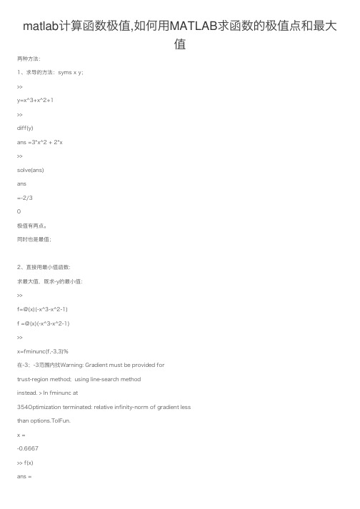
matlab计算函数极值,如何⽤MATLAB求函数的极值点和最⼤值两种⽅法：1、求导的⽅法：syms x y；>>y=x^3+x^2+1>>diff(y)ans =3*x^2 + 2*x>>solve(ans)ans=-2/3极值有两点。

同时也是最值；2、直接⽤最⼩值函数：求最⼤值，既求-y的最⼩值：>>f=@(x)(-x^3-x^2-1)f =@(x)(-x^3-x^2-1)>>x=fminunc(f,-3,3)%在-3；-3范围内找Warning: Gradient must be provided fortrust-region method; using line-search methodinstead. > In fminunc at354Optimization terminated: relative infinity-norm of gradient lessthan options.TolFun.x =-0.6667>> f(x)ans =-1.1481在规定范围内的最⼤值是1.1481由于函数的局限性，求出的极值可能是局部最⼩(⼤)值。

求全局最值要⽤遗传算法。

例⼦：syms xf=(200+5*x)*(0.65-x*0.01)-x*0.45;s=diff(f);%⼀阶导数s2=diff(f,2);%⼆阶导数h=double(solve(s));%⼀阶导数为零的点可能就是极值点，注意是可能，详情请见⾼数课本fori=1:length(h)ifsubs(s2,x,h(i))<0disp(['函数在' num2str(h(i))'处取得极⼤值，极⼤值为' num2str(subs(f,x,h(i)))])elseifsubs(s2,x,h(i))>0disp(['函数在' num2str(h(i))'处取得极⼩值，极⼩值为'num2str(subs(f,x,h(i)))])elsedisp(['函数在' num2str(h(i))'处⼆阶导数也为0，故在该点处函数可能有极⼤值、极⼩值或⽆极值'])%%%详情见⾼数课本endend。

高等数学：MATLAB实验

以上两种格式中的x、y都可以是表达式.plot是绘制二维曲线的基本函数,但在使用此函数之前,需先定义曲线上每一点的x及y的坐标.
MATLAB实验
2.fplot绘图命令 fplot绘图命令专门用于绘制一元函数曲线,格式为:
fplot('fun',[a,b]) 用于绘制区间[a,b]上的函数y=fun的图像.
MATLAB实验【实验内容】
MATLAB实验
由此可知,函数在点x=3处的二阶导数为6,所以f(3)=3为极小值;函数在点x= 1处的二阶导数为-6,所以f(1)=7为极大值.
MATLAB实验
例12-10 假设某种商品的需求量q 是单价p(单位:元)的函数q=12000-80p,商品的总成本C 是需求量q 的函数 C=25000+50q.每单位商品需要纳税2元,试求使销售利润达到最大的商品单价和最大利润额.
MATLAB实验
MATLAB实验
MATLAB实验
MATLAB实验
MATLAB实验
MATLAB实验
MATLAB实验
MATLAB实验
MATLAB实验实验九用 MATLAB求解二重积分
【实验目的】熟悉LAB中的int命令,会用int命令求解简单的二重积分.
MATLAB实验
【实验M步A骤T】由于二重积分可以化成二次积分来进行计算,因此只要
MATLAB实验
MATLAB实验
MATLAB实验
MATLAB实验
MATLAB实验
实验七应用 MATLAB绘制三维曲线图
【实验目的】 (1)熟悉 MATLAB软件的绘图功能; (2)熟悉常见空间曲线的作图方法.
【实验要求】 (1)掌握 MATLAB中绘图命令plot3和 mesh的使用; (2)会用plot3和 mesh函数绘制出某区间的三维曲线,线型

matlab求曲线极值程序,matlab函数求极值matlab函数求极值.ppt

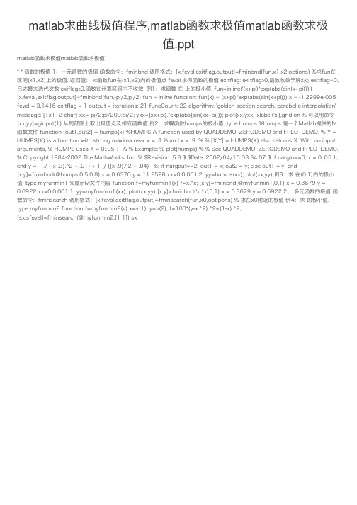
matlab求曲线极值程序,matlab函数求极值matlab函数求极值.pptmatlab函数求极值matlab函数求极值* * 函数的极值 1、⼀元函数的极值函数命令：fminbnd 调⽤格式：[x,feval,exitflag,output]=fminbnd(fun,x1,x2,options) %求fun在区间(x1,x2)上的极值. 返回值： x:函数fun在(x1,x2)内的极值点 feval:求得函数的极值 exitflag: exitflag>0,函数收敛于解x处 exitflag=0,已达最⼤迭代次数 exiflag<0,函数在计算区间内不收敛. 例1：求函数在上的极⼩值. fun=inline('(x+pi)*exp(abs(sin(x+pi)))')[x,feval,exitflag,output]=fminbnd(fun,-pi/2,pi/2) fun = Inline function: fun(x) = (x+pi)*exp(abs(sin(x+pi))) x = -1.2999e-005 feval = 3.1416 exitflag = 1 output = iterations: 21 funcCount: 22 algorithm: 'golden section search, parabolic interpolation' message: [1x112 char] xx=-pi/2:pi/200:pi/2; yxx=(xx+pi).*exp(abs(sin(xx+pi))); plot(xx,yxx) xlabel('x'),grid on % 可以⽤命令[xx,yy]=ginput(1) 从局部图上取出极值点及相应函数值例2：求解函数humps的极⼩值. type humps %humps 是⼀个Matlab提供的M 函数⽂件 function [out1,out2] = humps(x) %HUMPS A function used by QUADDEMO, ZERODEMO and FPLOTDEMO. % Y = HUMPS(X) is a function with strong maxima near x = .3 % and x = .9. % % [X,Y] = HUMPS(X) also returns X. With no input arguments, % HUMPS uses X = 0:.05:1. % % Example: % plot(humps) % % See QUADDEMO, ZERODEMO and FPLOTDEMO. % Copyright 1984-2002 The MathWorks, Inc. % $Revision: 5.8 $ $Date: 2002/04/15 03:34:07 $ if nargin==0, x = 0:.05:1; end y = 1 ./ ((x-.3).^2 + .01) + 1 ./ ((x-.9).^2 + .04) - 6; if nargout==2, out1 = x; out2 = y; else out1 = y; end[x,y]=fminbnd(@humps,0.5,0.8) x = 0.6370 y = 11.2528 xx=0:0.001:2; yy=humps(xx); plot(xx,yy) 例3：求在(0,1)内的极⼩值. type myfunmin1 %显⽰M⽂件内容 function f=myfunmin1(x) f=x.^x; [x,y]=fminbnd(@myfunmin1,0,1) x = 0.3679 y =0.6922 xx=0:0.001:1; yy=myfunmin1(xx); plot(xx,yy) [x,y]=fminbnd('x.^x',0,1) x = 0.3679 y = 0.6922 2、多元函数的极值函数命令：fminsearch 调⽤格式：[x,feval,exitflag,output]=fminsearch(fun,x0,optipons) % 求在x0附近的极值例4：求的极⼩值. type myfunmin2 function f=myfunmin2(v) x=v(1); y=v(2); f=100*(y-x.^2).^2+(1-x).^2;[sx,sfeval]=fminsearch(@myfunmin2,[1 1]) sx。

Matlab求解方程和函数极值

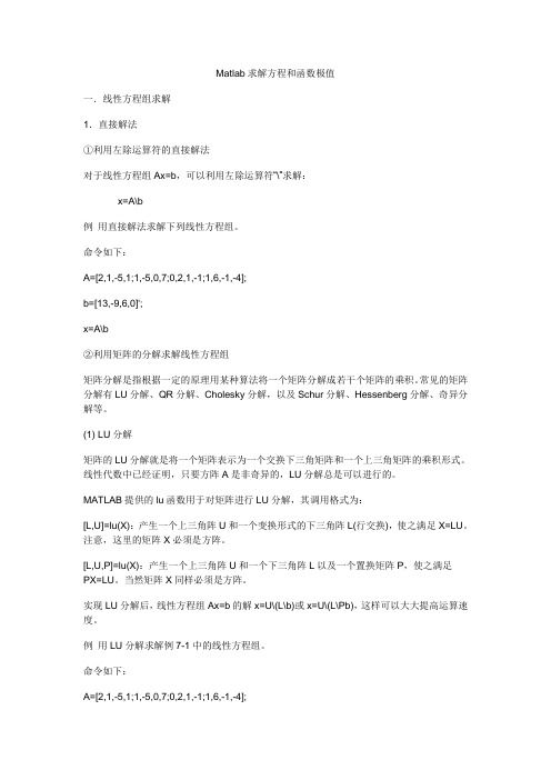
Matlab求解方程和函数极值一．线性方程组求解1．直接解法①利用左除运算符的直接解法对于线性方程组Ax=b，可以利用左除运算符“\”求解：x=A\b例用直接解法求解下列线性方程组。

命令如下：A=[2,1,-5,1;1,-5,0,7;0,2,1,-1;1,6,-1,-4];b=[13,-9,6,0]';x=A\b②利用矩阵的分解求解线性方程组矩阵分解是指根据一定的原理用某种算法将一个矩阵分解成若干个矩阵的乘积。

常见的矩阵分解有LU分解、QR分解、Cholesky分解，以及Schur分解、Hessenberg分解、奇异分解等。

(1) LU分解矩阵的LU分解就是将一个矩阵表示为一个交换下三角矩阵和一个上三角矩阵的乘积形式。

线性代数中已经证明，只要方阵A是非奇异的，LU分解总是可以进行的。

MATLAB提供的lu函数用于对矩阵进行LU分解，其调用格式为：[L,U]=lu(X)：产生一个上三角阵U和一个变换形式的下三角阵L(行交换)，使之满足X=LU。

注意，这里的矩阵X必须是方阵。

[L,U,P]=lu(X)：产生一个上三角阵U和一个下三角阵L以及一个置换矩阵P，使之满足PX=LU。

当然矩阵X同样必须是方阵。

实现LU分解后，线性方程组Ax=b的解x=U\(L\b)或x=U\(L\Pb)，这样可以大大提高运算速度。

例用LU分解求解例7-1中的线性方程组。

命令如下：A=[2,1,-5,1;1,-5,0,7;0,2,1,-1;1,6,-1,-4];b=[13,-9,6,0]';[L,U]=lu(A);x=U\(L\b)或采用LU分解的第2种格式，命令如下：[L,U ,P]=lu(A);x=U\(L\P*b)(2) QR分解对矩阵X进行QR分解，就是把X分解为一个正交矩阵Q和一个上三角矩阵R的乘积形式。

QR分解只能对方阵进行。

MATLAB的函数qr可用于对矩阵进行QR分解，其调用格式为：[Q,R]=qr(X)：产生一个一个正交矩阵Q和一个上三角矩阵R，使之满足X=QR。

matlab求导和极值

数学实验二用Matlab 软件求一元函数的导数和极（或最）值一、一元函数的导数1．调用格式一：diff(‘f(x)','x',n)式中，)(x f 为函数，x 为自变量，若未指明，按默认的自变量．n 为导数的阶数，缺省时，求一阶导数．例1 已知x x x f cos )(2=，求)(x f ′．解在命令行中输入：dydx=diff('x^2*cos(x)') %未指明自变量，按默认的自变量输出导数结果结果如下：dydx =2*x*cos(x)-x^2*sin(x)即x x x x x f sin cos 2)(2−=′．例2 已知)arcsin(xt t y =(x 为常数)，求22dty d ．解在命令行中输入：d2ydt2=diff('t*asin(x*t)','t',2) %若不指明对t 求导，则默认对x 求导结果如下：d2ydt2 =2*x/(1-x^2*t^2)^(1/2)+t^2*x^3/(1-x^2*t^2)^(3/2)即3223222])(1[)(12xt t x xt x dt y d −+−=． 2．调用格式二：syms xdiff(f(x),x,n)例3 已知)arcsin(xt t y =(t 为常数)，求2dx y d ．解在命令行中输入：syms x td2ydx2=diff(t*asin(x*t),x,2)输出结果是：d2ydx2 =t^4/(1-x^2*t^2)^(3/2)*x即32422])(1[xt xt dx y d −=．二、隐函数的导数在Matlab 中没有直接求隐函数导数的命令，但可调用Maple 中求隐函数导数的命令，调用格式如下：maple('implicitdiff(f(x,y)=0,y,x)')例4 求由方程05=−−+y x e xy 所确定的隐函数dxdy ．解在命令行中输入：dydx=maple('implicitdiff(x*y-exp(x+y)-5=0,y,x)')运行结果是：dydx =-(y-exp(x+y))/(x-exp(x+y))即 yx yx e x e y dx dy ++−−−=．三、一元函数的极（或最）值在Matlab 中只有求极（或最）小值命令的函数．若要求函数)(x f 在),(21x x 内的极（或最）大值，可转化为求)(x f −在),(21x x 内的极（或最）小值．求极（或最）小值点和极（或最）小值的调用格式是：[x,fual]=fminbnd(‘fun ’,x1,x2)式中，fun 为函数，x1，x2为x 的取值范围，x 为极（或最）小点，fual 为极（或最）小值．例5 求函数x e x f x sin 2)(−=在)5,2(的最小值点和最小值．解在命令行中输入：[xmin,fmin]=fminbnd('2*exp(-x)*sin(x)',2,5)输出结果如下：x min=3.9270fmin =-0.0279例6 求函数231)(x x x f −−=在]9,10[−的最值点和最值．解在命令行中输入：[xmin,fmin]=fminbnd('1-3*x-x^2',-10,9); %求)(x f 的最小值点和最小值[xmax,zmin]=fminbnd('-1+3*x+x^2',-10,9); %转化为求)(x f −的最小值点和最小值 fmax=-zmin; %))((x f −−的最大值xmin,fmin,xmax,fmax %输出最小值点、最小值和最大值点、最大值运行结果为：xmin =9fmin =-107xmax =-1.5000fmax =3.2500四、上机实验1．用help命令查看函数diff，fminbnd等的用法．2．上机验证上面各例．3．作相关小节练习中函数的导数和求函数的极（或最）值．。

matlab 符号极限

matlab 符号极限
在MATLAB中，你可以使用符号计算工具箱（Symbolic Math Toolbox）来处理符号极限。

以下是如何在MATLAB中计算符号极限的基本步骤：
1.定义符号变量：首先，你需要定义一个或多个符号变量。

2.创建符号表达式：使用这些符号变量来创建你想要的符号表达式。

3.计算极限：使用limit函数来计算表达式的极限。

下面是一个简单的例子，演示如何在MATLAB中计算符号极限：
matlab
% 1. 定义符号变量
syms x;
% 2. 创建符号表达式
f = sin(x) / x;
% 3. 计算极限
limitResult = limit(f, x, 0); % 计算 x 趋于 0 时的极限
% 显示结果
disp(limitResult);
在这个例子中，我们计算了sin(x) / x在x趋于0时的极限。

注意：要运行这些代码，你需要确保已经安装了符号计算工具箱。

如果你没有这个工具箱，MATLAB可能会报错。

用MATLAB求极值

用MATLAB求极值灵活的运用MATLAB的计算功能，可以很容易地求得函数的极值。

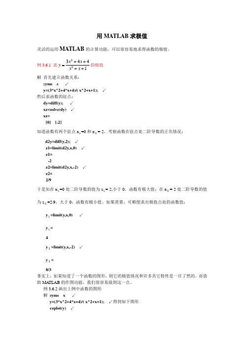
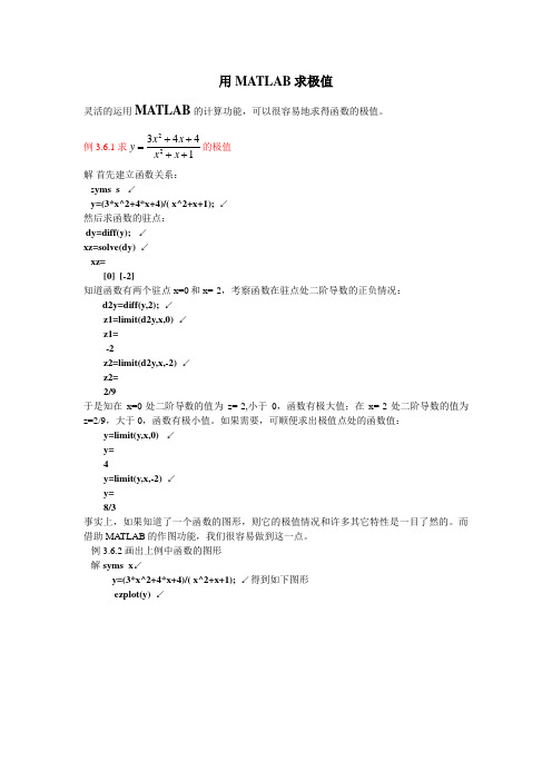
例3.6.1 求223441x xyx x++=++的极值解首先建立函数关系：s yms sy=(3*x^2+4*x+4)/( x^2+x+1); ↙然后求函数的驻点：dy=diff(y); ↙xz=solve(dy) ↙xz=[0] [-2]知道函数有两个驻点x1=0和x2=-2，考察函数在驻点处二阶导数的正负情况：d2y=diff(y,2); ↙z1=limit(d2y,x,0) ↙z1=-2z2=limit(d2y,x,-2) ↙z2=2/9于是知在x1=0处二阶导数的值为z1=-2,小于0，函数有极大值；在x2=-2处二阶导数的值为z2=2/9，大于0，函数有极小值。

如果需要，可顺便求出极值点处的函数值：y1=limit(y,x,0) ↙y1=4y2=limit(y,x,-2) ↙y2=8/3事实上，如果知道了一个函数的图形，则它的极值情况和许多其它特性是一目了然的。

而借助MA TLAB的作图功能，我们很容易做到这一点。

例3.6.2画出上例中函数的图形解syms x ↙y=(3*x^2+4*x+4)/( x^2+x+1); ↙得到如下图形ezplot(y) ↙如何用MATLAB求函数的极值点和最大值比如说y=x^3+x^2+1，怎样用matlab来算它的极值和最大值？求极值：syms x y>> y=x^3+x^2+1>> diff(y) %求导ans =3*x^2 + 2*x>> solve(ans)%求导函数为零的点ans =-2/3极值有两点。

求最大值，既求-y的最小值：>> f=@(x)(-x^3-x^2-1)f = @(x)(-x^3-x^2-1)>> x=fminunc(f,-3,3)% 在-3；-3范围内找Warning: Gradient must be provided for trust-region method;using line-search method instead.> In fminunc at 354Optimization terminated: relative infinity-norm of gradient less than options.TolFun.x =-0.6667>> f(x)ans =-1.1481在规定范围内的最大值是1.1481由于函数的局限性，求出的极值可能是局部最小（大）值。

MATLAB求函数零点与极值

MATLAB求函数零点与极值
1. roots函数
针对多项式求零点(详见MATLAB多项式及多项式拟合)
2. fzero函数
返回⼀元函数在某个区间内的的零点.
x0 = fzero(@(x)x.^2-3*x-4,[1,5]);
只能求区间⾥⾯的⼀个零点，并且要求在给定区间端点函数值异号，所以使⽤之前应该先作图，得出单个零点分布的区间，然后使⽤该函数求零点.若有多个零点，则需多次使⽤该函数.
如需求上例中的全部零点，先作图
fplot(@(x)x.^2-3*x-4,[-10,10]);
得知两个零点的分布区间，然后两次使⽤fzero函数求对应区间的零点.
x1 = fzero(@(x)x.^2-3*x-4,[-2,0]);
x2 = fzero(@(x)x.^2-3*x-4,[2,6]);
3. solve函数
求⼀元函数(⽅程)的零点.
x0 = solve('x^2-3*x-4=0','x');
注意⽅程需包含’=0’部分，另外，不建议直接将⽅程写在函数solve的参数部分，可以⽤符号运算的⽅法.
4. fminbnd函数
求⼀元函数在某个区间内的最⼩值和对应的最⼩值点.
[x0,fmin]=fminbnd(@(x)x+1/(x+1),-0.5,2);
求极值与极值点之前须估计极值点的区间，保证在该区间没有使得函数值趋于⽆穷的点.。

使用Matlab计算函数极限ppt课件

解：（1）输入： >> syms x
>> limit((exp(3*x)-1)/x,x,0)
按回车键，显示结果为： ans = 3
所以
l i me3x 1 x0 x
3
最新版整理ppt
10
（2）输入
>> clear
>> syms x
>> limit(((2*x+3)/(2*x+1))^(x+1),x,inf ) 按回车键，显示结果为 ans =exp(1)
Matlab计算函数极限
基础教学部数学教研室
2011.10
最新版整理ppt
1
主要内容
❖ 一元函数作图 ❖ 利用Matlab求极限 ❖ 练习
最新版整理ppt
2
§1.4.6 一元函数作图
绘图命令 fplot------是专门用于绘制一元函数曲线. 格式为：
fplot (’fun’,[a ,b]) 表示绘制区间 [a ,b]上函数 y=fun 的图形.
所以
lim( 2x 3)x1 e x 2 x 1
最新版整理ppt
返回
11
练习1.17
练习 1.17
求
lim
x0
(
1 x
)tan
x
解：输入： >> clear
>> syms x
>>
limit((1/x)^tan(x),x,0,'right') 按回车键，显示结果为： ans =1
所以
l
i
1 m
练习1.15
最新版整理ppt
3
§1.4.7 利用MATLAB求极限

Matlab求解方程和函数极值.docx

Mat lab求解方程和函数极值The fifth chapter, 22010-03-31 22:50Two. Matlab for solving equations and function extremumI. solving linear equations1. direct solutionThe direct solution to the use of the left division operatorFor linear equations Ax=b, we can use the left division operator to solve: X=A\bFor example, the following linear equations are solved by direct solution. The commands are as follows:A=[2, 1, -5, 1; 1; -5,0,7; 0,2, 1; -1; 1,6; -1; —4];B=[13, -9,6,0]，;X=A\bSolving linear equations by the decomposition of matrixMatrix decomposition is the product of decomposing a matrix into several matrices according to certain principles・ Common matrix decomposition includes LU decomposition, QR decomposition, Cholesky decomposition, and Schur decomposition, Hessenberg decomposition, singular decomposition,and so on.(1)LU decompositionThe LU decomposition of a matrix means that a matrix is expressed as a product of a commutative lower triangular matrix and an upper triangular matrix・Linear algebra has proved that LU decomposition is always possible as long as the square A is nonsingular・\IATLAB provides the Lu function for LU decomposition of the matrix, the call format for:[L, U]二lu (X): produces an upper triangular array U and a transform form of lower triangular array L (row exchange) to satisfy X二LU. Note that the matrix X here must be square・[L, U, P]二lu (X): produces an upper triangular array U and a lower triangular matrix L, and a permutation matrix P, which satisfies PX=LU ・ Of course, the matrix X must also be square・After the LU decomposition, the solution of the linear equations Ax二b (L\b) or x二U\ (L\Pb), which can greatly improve the speed of operation x二U\・For example, LU is used to solve the linear equations in example 7-1. The commands are as follows:A二[2,1, -5, 1; 1; -5,0,7; 0,2, 1； T； 1,6; -1; -4];B二[13, -9, 6,0]';[L, U]二lu (A);X二U\ (L\b)Or using LU decomposition of the second formats, as follows:[L, U, P]二lu (A);X二U\ (L\P*b)(2)QR decompositionQR decomposition of the matrix X, is the decomposition of X into an orthogonal matrix Q and an upper triangular matrix R product form. QR decomposition can only be carried out by the opponent，s array. MATLAB function QR can be used for QR decomposition of the matrix, the call format for:[Q, R]=qr (X): produces an orthogonal matrix Q and an upper triangular matrix R so that it satisfies X二QR・[Q, R, E]=qr (X): produce an orthogonal matrix Q, an upper triangular matrix, R, and a permutation matrix E, so that it satisfies XE二QR.After the QR decomposition, the solution of the linear equation Ax二b is x二R\ (Q\b) or x二E (R\ (Q\b))・For example, QR is used to solve the linear equations in example 7-1.The commands are as follows:A二[2,1, -5, 1; 1; -5,0,7; 0,2, 1； T； 1,6; -1; -4];B二[13, -9, 6,0]';[Q, R]二qr (A);X二R\ (Q\b)Or using QR decomposition of the second formats, as follows:[Q, R, E] =qr (A):X二E* (R\ (Q\b))(3)Cholesky decompositionIf the matrix X is symmetric and positive definite, the Cholesky decomposition decomposes the matrix X into the product of a lower triangular matrix and upper triangular matrix・ Set the triangle matrix to R,Then the lower triangular matrix is transposed, that is, X二R' R・ The MATLAB function Choi (X) is used for Cholesky decompositionof the matrix X, and its call format is:R二chol (X): produces an upper triangular array R that makes R'R二X ・If the X is an asymmetric positive definite, an error message is output ・[R, p]二chol (X): this command format will not output error messages・ When X is symmetric positive definite, then p二0 and R are the same as those obtained in the above format: otherwise, P is a positive integer ・If X is a full rank matrix, then R is an upper triangular matrix of order q=p-l and satisfies R'R二X (l：q, l：q)・After the Cholesky decomposition, the linear equation group Ax二b becomes R 'Rx二b, so x二R\ (R， \b ')・Example 4 decomposes the system of linear equations in example 7-1 by Cholesky decomposition.The commands are as follows:A二[2,1, -5, 1; 1; -5, 0,7; 0,2, 1； T； 1,6; -1; -4];B 二[13, —9,6,0]';R二chol (A)Error using Chol =>???Matrix, must, be, positive, definiteWhen the command is executed, an error message appears indicating that the A is a non positive definite matrix・2. iteration methodIterative method is very suitable for solving large coefficient matrix equations・ In numerical analysis, the iterative methods mainly include Jacobi iterative method, Gauss-Serdel iterative method, over relaxationiterative method and two step iterative method・Jacobi iteration methodFor linear equations Ax二b, if A is a nonsingular square, that is, (i=l, 2,・・・(n), A can be decomposed into A 二D-L-U, where D is a diagonal matrix, and its elements are diagonal elements of A, L and U are lower triangular and upper triangular matrices of A, so Ax二b becomes・・:The corresponding iteration formula is:This is the Jacobi iteration formula・If the sequence converges to x, then x must be the solution of equation Ax二b・The MATLAB function file of the Jacobi iteration method Jacobi.m is as follows:Function, [y, n]二jacobi (A, B, xO, EPS)If nargin=3Eps=1.Oe-6;Elseif nargin〈3ErrorReturnEndD=diag (diag (A)) -% A diagonal matrixL=-tril (A, -1); the lower triangular array of% AU二-triu (A, 1); the upper triangular array of% AB二D\ (L+U);F二D\b;Y二B*xO+f:N二1;% iterationsWhile norm (y-xO) 〉=epsXO二y;Y二B*xO+f:N二n+1;EndExample 5 uses the Jacobi iterative method to solve the following linear equations・The initial value of iteration is 0, and the iteration accuracy is 10-6・Call the function file "Jacobi.nT in the command. The command is as follows:A二[10, -1,0; -1, 10; -2; 0; -2, 10];B二[9, 7,6]';[x, n]二jacobi (A, B, [0,0,0]', 1. Oe-6)Gauss-Serdel iteration methodIn the Jacobi iteration process, the calculations have been obtained and need not be reused, i.e., the original iterative formula Dx (k+1)二(L+U) x (k) +b can be improved to Dx (k+1) 二Lx (k+1) +Ux (k) +b and thus obtained:X (k+1)二(D-L) -lUx (k) + (D-L) TbThis formula is the Gauss-Serdel iterative formula・ Compared with the Jacobi iteration,The Gauss-Serdel iteration replaces the old components with new ones, with higher accuracy・The MATLAB function f订e of the Gauss-Serdel iteration method gauseidel.m is as follows:Function, [y, n]=gauseidel (A, B, xO, EPS)If nargin=3Eps二1. 0e-6;Elseif nargin<3ErrorReturnEndD=diag (diag (A)) -% A diagonal matrixL=-tril (A, -1); the lower triangular array of% AU=-triu (A, 1); the upper triangular array of% AG二(D-L) \U;F二(D-L) \b;Y二G*xO+f;N=l;% iterationsWhile norm (y-xO) >=epsXO二y;Y二G*xO+f:N二n+1;EndExample 6 uses the Gauss-Serdel iterative method to solve the followinglinear equations・The initial value of iteration is 0, and the iteration accuracy is 10-6・Call the function file z，gauseidel.m" in the command. The command is as follows:A二[10, -1,0; -1, 10; -2; 0; -2, 10];B二[9, 7,6]';[x, n]二gauseidel (A, B, [0,0,0]', 1.0e~6)Example 7, Jacobi iteration and Gauss-Serdel iteration method are used to solve the following linear equations, to see whether convergence・The commands are as follows:A二[1,2, -2; 1, 1, 1; 2, 2,11；B二[9; 7; 6];[x, n]=jacobi (a, B, [0; 0; 0])[x, n]=gauseidel (a, B, [0; 0; 0])Two. Numerical solution of nonlinear equations1 solving the single variable nonlinear equationIn MATLAB, a fzero function is provided that can be used to find the roots of a single variable nonlinear equation. The call format of this functionis: z二fzero ('fname', xO, tol, trace)Where fname is the root to be a function of the file name, xO as the search starting point・ A function may have more than one root, but the fzero function only gives the root nearest to the x0・ The relative accuracy of the TOL control results, by default, take tol二eps, trace, specify whether the iteration information is displayed in the operation, and when 1 is displayed, 0 is not displayed, and the trace=0 is taken by default・Example 8 ask for roots in the neighborhood.Steps are as follows:(1) establishment of function file funx・m.Function fx二funx (x)Fx二xTO. x+2;(2) fzero function call root.Z=fzero (' funx', 0. 5)二ZZero point three seven five eight2. solving nonlinear equationsFor nonlinear equations F (X) =0, the numerical solution is obtained by using the fsolve function. The call format of the fsolve function is:X二fsolve (' fun，, X0, option)Where X is the return of the solution, fun is used to define the demand for solutions of nonlinear equations function of the file name, X0 is the initial rooting process, option optimization toolbox options・ The Optimization Toolbox provides more than 20 options that users can display using the optimset command・If you want to change one of the options, you can call the optimset () function to complete it. For example, Display display option decision function calls intermediate results, in eluding 〃off〃does not show, 〃ITER〃said each show,'final5 shows only the final results・ Optimset ('Display', 'off') will set the Display option to 'off'.Example 9 find the numerical solution of the following nonlinear equations in (0.5,0.5) neighborhood・(1)establishment of function file myfun. m.Function q=myfun (P)X二p (1);Y二p (2);Q (1) =x-0・6*sin (x) -0.3*cos (Y);Q (2)二y-0・6*cos (x) +0. 3*sin (Y);(2)under the given initial value x0=0・5 and y0=0・5, call the fsolve function to find the root of the equation.X二fsolve C myfun，, [0.5,0. 5]', optimset ('Display'off'))二xZero point six three five fourZero point three seven three fourThe solution is returned to the original equation, and it can be checked whether the result is correct or not:Q二myfun (x)1.0e-009 *0. 2375, 0. 2957We can see the result of higher precision.Three・ Numerical solution of initial value problems for ordinary differential equations1. introduction of Runge Kutta method2., the realization of Runge Kutta methodBased on Runge Kutta method, MATLAB provides the function of finding numerical solutions of ordinary differential equations:[t, y]二ode23 C fname，, tspan, Y0)[t, y]二ode45 C fname，, tspan, Y0)Where fname is the function file name that defines f (T, y), and the function file must return a column vector・ The tspan form is [tO, tf], which represents the solution interva. 1. Y0 is the initial state column vector ・ The time vectors and corresponding state vectors are given by T and Y respectively.Example 10 has an initial value problem,Try to find the numerical solution and compare it with the exact solution (the exact solution is y (T)二).(1)establishment of function file funt. m.Function yp二funt (T, y)Yp= (y"2-t-2) /4/ (t+1);(2)solving differential equations・TOO; tf二10;¥0=2;[t, y]=ode23 ('funt', [tO, tf], Y0) ;% for numerical solutionYl=sqrt (t+1) +1;% refinement; exact solutionPlot (T, y, 'B・'，t, Yl, ?)% are compared by graphThe numerical solution is represented by a blue dot, and the exact solution is expressed in red solid lines・ As shown. It can be seen that the two results approximate・ CloseFour. Function extremumMATLAB provides functions based on the simplex algorithm for solving extremal functions Fmin and fmins, which are used respectively for minimum values of univariate functions and multivariate functions:X二fmin (' fname，, xl, x2)X二fmins (' fname' , xO)The call formats of the two functions are similar・ Among them, the Fmin function is used to find the minimum point of a single variable function. Fname is the object function name that is minimized, and XI and X2 limit the range of arguments・ The fmins function is used to find the minimum point of a multivariable function, and xO is the initial value vector of the solution.MATLAB provides no special function to find the maximum function, but as long as the attention to -f (x) in the interval (a, b) is the minimum value of F (x) in (a, b) of the maximum value, so Fmin (F, xl, x2) f (x) function in the interval (xl the maximum value, X2)・Example 13 asks in [0,Minimum point in 5]・(1)establishment of function file mymin. m.Function fx二mymin (x)Fx=x.八3-2*x-5;(2)call the Fmin function to find the minimum point・Zero point eight one six fiveThree・Matlab numerical integration and differentiationI. numerical integration1.basic principles of numerical integrationNumerical methods for solving definite integration are various, such as simple trapezoidal method, Xin Pusheng (Simpson) method, Newton Cortes (Newton-Cotes) method, etc・,are often used・Their basic idea is to divide the whole integral interval [a and b] into n sub intervals [[, ], i=l, 2],・・・ N, in which,・ In this way, the problem of determining integral is decomposed into summation problem・2.realization method of numerical integrationVariable step symplectic methodBased on the variable step long Xin Pusheng method, MATLAB gives the quad function to find the definite integra 1. The call format of this function is:[I, n]二quad ('fname', a, B, tol, trace)Where fname is the product function name・A and B are the lower bound and upper bound of the definite integra 1. TOL is used to control the integration accuracy, and the tol=0.001 is taken by default・ Does the trace control show the integration process? If you take the non 0, it will show the integral process, take 0 instead of the default, and take the trace=0 bydefault・ Returns the parameter I, the fixed integral value, and the call number of n for the integrand・Finding definite integral(1)establish the integrand function file fesin.m.Function f二fesin (x)F二exp (一0.5*x)・ *sin (x+pi/6);(2)call the numerical integral function quad to find the definite integra1.[S, n]二quad ('fesin', 0, 3*pi)二SZero point nine Zero Zero eight二nSeventy-sevenThe Newton Cotes methodNewton Cotes method based on MATLAB, gives the quad8 function to find the definite integra 1. The call format of this functionis: [I, n]=quad8 C fname，, a, B, tol, trace)The meaning of the parameter is similar to that of the quad function, but only the default value of the tol. The function can more accurately calculate the value of the definite integral, and in general, the number of steps of the function call is less than the quad function, thus ensuring the higher efficiency to find the required integral value・Finding definite integral(1)the integrand function file fx. m・Function f二fx (x)F二x. *sin (x) / (1+cos (x)・*cos (x));(2)call the function quad8 to find the definite integral.I二quad8 (' fx' , 0, PI)二ITwo point four six seven fourExample 3 uses the quad function and the quad8 function respectively to find the approximate value of the integral, and compares the number of calls of the function under the same integral accuracy.Call the function quad to find the definite integral:Format long;Fx二inline ('exp (-x));[I, n]二quad ('FX', 1,2. 5, le-10)二IZero point two eight five seven nine four four four two fivefour seven six six二nSixty-fiveCall the function quad8 to find the definite integral:Format long;Fx二inline ('exp (-x));[I, n] =quad8 (FX, 1,2. 5, le-10)二IZero point two eight five seven nine four four four two fivefour seven five fourThirty-threeThe integrand is defined by a tableIn MATLAB, the problem of determining the function relations defined in tabular form is called trapz (X, Y) functions. The vector X, Y defines the function relation Y二f (X).Example 8-4 calculates definite integral with trapz function.The commands are as follows:X=l:0. 01:2.5：Y二exp (-X);% generated function relational data vectorTrapz (X, Y)二ansZero point two eight five seven nine six eight two four one six three nine threeNumerical solution of 3. double definite integralConsider the following double definite integral problem:By using the dblquad function provided by MATLAB, the numerical solution of the above double definite integral can be obtaineddirectly. The call format of this function is:I=dblquad (F, a, B, C, D, tol, trace)The function asks f (x, y) to double definite integral on the [a, b] * [c, d] regions・The parameter tol, trace is used exactly the same as function quad・Example 8~5 calculates the double definite integral(1)build a function file fxy.m:Function f二fxy (x, y)Global ki;Ki=ki+1:%ki is used to count the number of calls to the integrandF二exp (-x.八2/2). *sin (x. 2+y);(2)call the dblquad function to solve・Global ki; ki二0;I二dblquad (' fxy' , -2, 2, -1, 1)Ki1.57449318974494 (data format related)二kiOne thousand and thirty-eightTwo. Numerical differentiation1numerical difference and difference quotient2the realization of numerical differentiationIn MATLAB, there is no function that provides direct numerical derivatives・ Only the function diff, which calculates the forward difference, is called:DX二diff (X) : calculates the forward difference of vector X, DX (I), =X (i+1), -X (I), i二1,2,・・.N-l.DX二diff (X, n) : calculates the forward difference of the n order of X. For example, diff (X, 2)二diff (diff (X)).DX二diff (A, N, dim): calculates the n order difference of the matrix A, the dim=l (default state), calculates the difference by column, and dim=2 calculates the difference by line・6 cases of Vandermonde matrix generation based on vectorV= [ 1, 2, 3, 4, 5, 6], according to the column difference operation. The commands are as follows:V=vander (1:6)DV二diff (V)% calculates the first order difference of V 二V111111321684212438127931102425664164131256251252551777612962163661二DV31157310211 65 19 5 1 0781 175 37 7 1 02101 369 61 9 1 04651 671 91 11 1 0用不同的方法求函数f(X)的数值导数，并在同一个坐标系中做出f (X)的图像。

matlab多项式运算及求极限、复杂函数求极限

文章主题：深入探讨MATLAB中的多项式运算及求极限、复杂函数求极限MATLAB（Matrix Laboratory）是一款强大的数学软件，广泛应用于工程、科学、经济等领域。

在MATLAB中，多项式运算及求极限、复杂函数求极限是常见且重要的数学问题，对于提高数学建模和计算能力具有重要意义。

本文将从简到繁地探讨MATLAB中的多项式运算及求极限、复杂函数求极限，以帮助读者深入理解这一主题。

一、MATLAB中的多项式运算多项式是数学中常见的代数表达式，通常以系数的形式表示。

在MATLAB中，可以使用多种方法进行多项式的运算，如加法、减法、乘法、除法等。

对于两个多项式f(x)和g(x)，可以使用“+”、“-”、“*”、“/”等运算符进行运算。

在实际应用中，多项式的运算往往涉及到多项式系数的提取、多项式的乘方、多项式的符号变化等操作。

MATLAB提供了丰富的函数和工具箱，如polyval、polyfit、roots等，可以帮助用户进行多项式的运算。

通过这些工具，用户可以方便地进行多项式的求值、拟合、求根等操作。

二、MATLAB中的多项式求极限求多项式的极限是微积分中常见的问题，对于研究函数的性质和图像具有重要意义。

在MATLAB中，可以通过lim函数来求多项式的极限。

lim函数可以接受不同的输入参数，如函数、变量、极限点等，从而计算多项式在某一点的极限值。

在进行多项式求极限时，需要注意的是对极限的性质和运算规则。

MATLAB中的lim函数遵循了标准的极限计算规则，如极限的四则运算法则、极限的有界性、极限的夹逼定理等。

用户可以通过lim函数灵活地进行多项式求极限的计算和分析。

三、MATLAB中的复杂函数求极限除了多项式，复杂函数在工程和科学中也具有广泛的应用。

MATLAB提供了丰富的函数和工具箱，如syms、limit、diff等，可以帮助用户进行复杂函数的求导、求极限等操作。

对于复杂函数的极限计算，需要综合运用代数运算、微分计算、极限性质等技巧。

用MATLAB求极值

用MATLAB求极值灵活的运用MATLAB的计算功能，可以很容易地求得函数的极值。

例3.6.1 求223441x xyx x++=++的极值解首先建立函数关系：s yms s ↙y=(3*x^2+4*x+4)/( x^2+x+1); ↙然后求函数的驻点：dy=diff(y); ↙xz=solve(dy) ↙xz=[0] [-2]知道函数有两个驻点x1=0和x2=-2，考察函数在驻点处二阶导数的正负情况：d2y=diff(y,2); ↙z1=limit(d2y,x,0) ↙z1=-2z2=limit(d2y,x,-2) ↙z2=2/9于是知在x1=0处二阶导数的值为z1=-2,小于0，函数有极大值；在x2=-2处二阶导数的值为z2=2/9，大于0，函数有极小值。

而借助MA TLAB的作图功能，我们很容易做到这一点。

求最大值，既求-y的最小值：>> f=@(x)(-x^3-x^2-1)f =@(x)(-x^3-x^2-1)>> x=fminunc(f,-3,3)% 在-3；-3范围内找Warning: Gradient must be provided for trust-region method;using line-search method instead.> In fminunc at 354Optimization terminated: relative infinity-norm of gradient less than options.TolFun.x =-0.6667>> f(x)ans =-1.1481在规定范围内的最大值是1.1481由于函数的局限性，求出的极值可能是局部最小（大）值。

MATLAB实验报告3-符号运算

>> F=subs(gy,{x,y},{x-1,y-2})
F =
((x - 1)^3 - 5)/(2*(x - 1)^2 + 7)
2）
>> clear
>> syms x y;
>> g=(x^3*y-5*y)/(2*x^2+7);
>> gxy=diff(diff(g,x),y);
>> G=subs(gxy,{x},{x-1})
>> int(y)
ans =
log(x + 1)
>> int(y,0,1)
ans =
log(2)
>> syms t;
>> int(y,0,t)
ans =
log(t + 1)
>> clear
>> syms x y;
>> z=sin(y)/(x^2*y+1);
>> int(z,-inf,+inf)
ans =
8.积分中值定理：设 ,存在 ,使得 .检验存在，使得 .
四、实验步骤和运行结果（如运行有错误，请指出）
1.
>> syms u v x;
>> f=sqrt(1+u^2);
>> g=log(v);
>> h=exp(-x);
>> p=compose(g,h)
p =
log(exp(-x))
>> compose(f,p)
(pi*sin(y))/y^(1/2)

matlab 实验3 函数的极值以及符号表达式的计算

实验3 函数的极值以及符号表达式的计算一、实验目的1、求函数的极值；2、符号表达式的分解、展开与化简；3、求符号表达式的极限；4、级数的求和与泰勒级数展开。

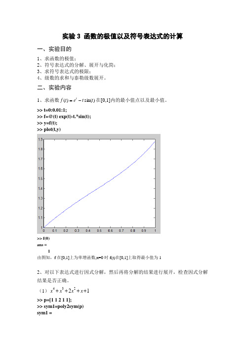
二、实验内容1、求函数)sin()(t t e t f t -=在[0,1]内的最小值点以及最小值。

>> t=0:0.01:1;>> f=@(t) exp(t)-t.*sin(t);>> y=f(t); >> plot(t,y)>> f(0)ans =1由图知，f 在[0,1]上为单增函数,x=0时f(t)在[0,1]上取得最小值为12、对以下表达式进行因式分解，然后再将分解的结果进行展开，检查因式分解结果是否正确。

（1）12234++++x x x x>> p=[1 1 2 1 1];>> sym1=poly2sym(p)sym1 =x^4 + x^3 + 2*x^2 + x + 1>> sym2=factor(sym1)sym2 =(x^2 + 1)*(x^2 + x + 1)>> sym3=expand(sym2)sym3 =x^4 + x^3 + 2*x^2 + x + 1（2）6555234-++-x x x x>> p=[1 -5 5 5 -6];>> sym1=poly2sym(p)sym1 =x^4 - 5*x^3 + 5*x^2 + 5*x - 6>> sym2=factor(sym1)sym2 =(x - 1)*(x - 2)*(x - 3)*(x + 1)>> sym3=expand(sym2)sym3 =x^4 - 5*x^3 + 5*x^2 + 5*x – 63、对以下表达式进行化简。

（1）123842+++x x x >> syms x>> y=(4*x.^2+8*x+3)/(2*x+1); >> simple(y)ans =2*x + 3（2）x x 22sin cos 2->> syms x>> y=2*cos(x).^2-sin(x).^2y =2*cos(x)^2 - sin(x)^2>> simple(y)ans =2 - 3*sin(x)^24、求下列函数的极限。

用MATLAB求极值

用MATLAB求极值灵活的运用MATLAB的计算功能，可以很容易地求得函数的极值。

例3.6.1 求223441x xyx x++=++的极值解首先建立函数关系：s yms s ↙y=(3*x^2+4*x+4)/( x^2+x+1); ↙然后求函数的驻点：dy=diff(y); ↙xz=solve(dy) ↙xz=[0] [-2]知道函数有两个驻点x=0和x=-2，考察函数在驻点处二阶导数的正负情况：d2y=diff(y,2); ↙z1=limit(d2y,x,0) ↙z1=-2z2=limit(d2y,x,-2) ↙z2=2/9于是知在x=0处二阶导数的值为z=-2,小于0，函数有极大值；在x=-2处二阶导数的值为z=2/9，大于0，函数有极小值。

如果需要，可顺便求出极值点处的函数值：y=limit(y,x,0) ↙y=4y=limit(y,x,-2) ↙y=8/3事实上，如果知道了一个函数的图形，则它的极值情况和许多其它特性是一目了然的。

而借助MATLAB的作图功能，我们很容易做到这一点。

例3.6.2画出上例中函数的图形解syms x↙y=(3*x^2+4*x+4)/( x^2+x+1); ↙得到如下图形ezplot(y) ↙如何用MATLAB求函数的极值点和最大值比如说y=x^3+x^2+1，怎样用matlab来算它的极值和最大值？求极值：syms x y>> y=x^3+x^2+1>> diff(y) %求导ans =3*x^2 + 2*x>> solve(ans)%求导函数为零的点ans =-2/3极值有两点。

求最大值，既求-y的最小值：>> f=@(x)(-x^3-x^2-1)f =@(x)(-x^3-x^2-1)>> x=fminunc(f,-3,3)% 在-3；-3范围内找Warning: Gradient must be provided for trust-region method;using line-search method instead.> In fminunc at 354Optimization terminated: relative infinity-norm of gradient less than options.TolFun.x =-0.6667>> f(x)ans =-1.1481在规定范围内的最大值是1.1481由于函数的局限性，求出的极值可能是局部最小（大）值。

matlab计算函数最大值及最小值

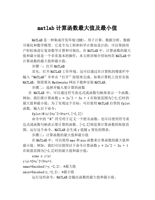
matlab计算函数最大值及最小值MATLAB是一种集成开发环境(IDE)，用于计算、数据分析、数据可视化和数学模型。

它是专为工程和科学计算而设计的，可以帮助用户轻松地进行复杂数学计算和可视化。

在MATLAB中，计算函数的最大值和最小值是一个非常基本的操作，本文将详细介绍如何在MATLAB中计算函数的最大值和最小值。

步骤一：打开MATLAB首先，打开MATLAB工作环境。

这可以通过在计算机的搜索栏中输入“MATLAB”并单击“打开”按钮来完成。

如果计算机上没有安装MATLAB，则需要从Mathworks网站下载和安装MATLAB。

步骤二：选择并输入要计算的函数在MATLAB中，可以通过符号表达式或函数句柄来表示一个函数。

例如，我们要计算函数y = 2x^2 - 3x + 4在取值范围为[-2,2]时的最大值和最小值。

为了实现这个目标，可以使用MATLAB自带的fplot 函数。

输入以下命令：fplot(@(x)2*x^2-3*x+4,[-2,2])命令中的“@”符号用于定义一个匿名函数，也可以使用符号表达式或函数句柄表示要计算的函数。

[-2,2]则是要计算函数的取值范围。

运行这个命令，MATLAB会生成y值随x变化的图表。

步骤三：计算函数的最大值和最小值在MATLAB中，可以使用max和min函数来计算函数的最大值和最小值。

例如，我们可以使用以下命令计算函数y = 2x^2 - 3x + 4在取值范围为[-2,2]时的最大值和最小值：syms x y(x)y(x)=2*x^2-3*x+4;xmax=fminbnd(-y,-2,2); #最大值xmin=fminbnd(y,-2,2); #最小值运行这些命令，MATLAB会输出函数的最大值和最小值。

至此，我们完成了计算函数的最大值和最小值的过程。

以上步骤也可以通过matlab自带的3D画图工具箱实现更快捷的展示方式。

这只是MATLAB功能的一部分，MATLAB的强大功能可以帮助用户在数学计算、数据分析和数据可视化方面取得更好的成果。

matlab多元函数求极值

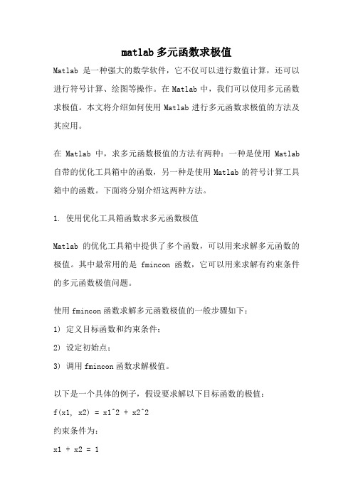
matlab多元函数求极值Matlab是一种强大的数学软件，它不仅可以进行数值计算，还可以进行符号计算、绘图等操作。

在Matlab中，我们可以使用多元函数求极值。

本文将介绍如何使用Matlab进行多元函数求极值的方法及其应用。

在Matlab中，求多元函数极值的方法有两种：一种是使用Matlab 自带的优化工具箱中的函数，另一种是使用Matlab的符号计算工具箱中的函数。

下面将分别介绍这两种方法。

1. 使用优化工具箱函数求多元函数极值Matlab的优化工具箱中提供了多个函数，可以用来求解多元函数的极值。

其中最常用的是fmincon函数，它可以用来求解有约束条件的多元函数极值问题。

使用fmincon函数求解多元函数极值的一般步骤如下：1) 定义目标函数和约束条件；2) 设定初始点；3) 调用fmincon函数求解极值。

以下是一个具体的例子，假设要求解以下目标函数的极值：f(x1, x2) = x1^2 + x2^2约束条件为：x1 + x2 = 1定义目标函数和约束条件：function f = objfun(x)f = x(1)^2 + x(2)^2;endfunction [c,ceq] = confun(x)c = [];ceq = x(1) + x(2) - 1;end然后，设定初始点：x0 = [0, 0];调用fmincon函数求解极值：options = optimoptions('fmincon','Display','iter');[x,fval] = fmincon(@objfun,x0,[],[],[],[],[],[],@confun,options);其中，options用于设定一些选项，如是否显示迭代过程等。

2. 使用符号计算工具箱函数求多元函数极值除了使用优化工具箱函数，Matlab的符号计算工具箱中也提供了一些函数，可以用来求解多元函数的极值。

实验3Matlab符号运算及求函数极值

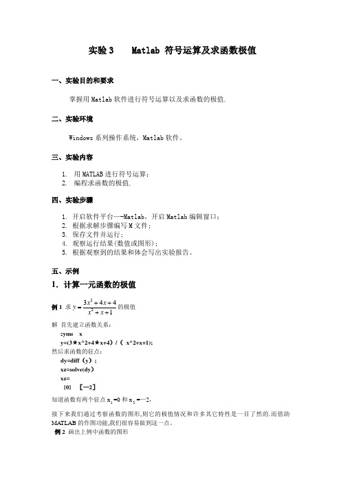
实验3 Matlab 符号运算及求函数极值一、实验目的和要求掌握用Matlab软件进行符号运算以及求函数的极值.二、实验环境Windows系列操作系统，Matlab软件。

三、实验内容1.用MATLAB进行符号运算；2.编程求函数的极值.四、实验步骤1.开启软件平台—-Matlab，开启Matlab编辑窗口；2.根据求解步骤编写M文件;3.保存文件并运行;4.观察运行结果(数值或图形);5.根据观察到的结果和体会写出实验报告。

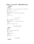
五、示例1．计算一元函数的极值例1求223441x xyx x++=++的极值解首先建立函数关系：s yms xy=(3＊x^2+4＊x+4）/（x^2+x+1); 然后求函数的驻点：dy=diff（y）;xz=solve(dy）xz=[0] ［—2］知道函数有两个驻点x1=0和x2=—2，接下来我们通过考察函数的图形,则它的极值情况和许多其它特性是一目了然的.而借助MATLAB的作图功能,我们很容易做到这一点。

例2 画出上例中函数的图形解 syms xy=（3*x^2+4*x+4）/( x^2+x+1）；得到如下图形ezplot(y ）2．计算二元函数的极值MATLAB 中主要用diff 求函数的偏导数,用jacobian 求Jacobian 矩阵。

diff （f,x ，n) 求函数f 关于自变量x 的n 阶导数.jacobian(f ，x ）求向量函数f 关于自变量x(x 也为向量)的jacobian矩阵.可以用help diff ， help jacobian 查阅有关这些命令的详细信息例1 求函数42823z x xy y =-+-的极值点和极值。

首先用diff 命令求z 关于x ，y 的偏导数〉〉clear; syms x y;〉〉z=x^4-8*x ＊y+2＊y^2—3；>〉diff(z,x ）>>diff(z ，y)结果为ans =4*x^3—8＊yans =-8＊x+4*y即348,84z z x y x y x y∂∂=-=-+∂∂再求解方程，求得各驻点的坐标。

matlab复杂函数求极限

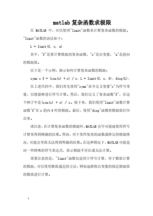
matlab复杂函数求极限
在MATLAB中，可以使用"limit"函数来计算复杂函数的极限。

"limit"函数的语法如下：
L = limit(f, x, a)
其中，"f"是要计算极限的复杂函数，"x"是自变量，"a"是趋向的极限值。

以下是一个示例，演示如何计算复杂函数的极限：
syms x f = (sin(x) + x) / x; L = limit(f, x, 0); disp(L);
在上述代码中，我们首先使用"syms"命令定义变量"x"为符号变量，以便能够进行符号计算。

然后，我们定义了复杂函数"f"，在这个例子中是(sin(x) + x) / x。

接下来，我们使用"limit"函数计算函数"f"在x趋向0时的极限。

最后，使用"disp"函数将极限值打印出来。

请注意，在计算复杂函数的极限时，MATLAB会尽可能地使用符号计算来得到精确的结果。

然而，对于某些复杂的函数或特定的极限情况，可能会导致无法得到明确的结果。

在这种情况下，MATLAB可能返回一些特殊的符号表达式，表示极限不存在或无法计算。

需要注意的是，"limit"函数仅适用于符号计算，对于数值计算的极限，可以使用数值逼近的方法，例如逐渐取自变量的接近极限值的数值进行计算。

1。

Matlab求极限

limit((x^2-1)/(x-1),x,1) limit((x^2-1)/(x-1),x,1)
limit (y,x,1)
例2：
求
lim(1-
x
x 2
)(
x
3)
解：clear
syms x
y=(1-x/2)^(x+3)
limit(y,x ,inf)
例3：求lim 1 x x0
解：clear
Matlab求极限
1、符号变量和符号表达式 2、MATLAB下求极限运算的格式和方法
１、符合对象和符号表达式
在进行符号计算时，首先要定义基本的符号对象，然后里用这些基本的符号对象去构成符号表达式。
例如：我们要在matlab命令窗口中输入
x2 1
x 1
我们首先要告诉计算机x是一个符号，
然后这个符合和常数构成符号表达式 x2 1 x 1
lim f (x)
xa
limit(f,x,a,’left’) 左极限
lim f (x)
xa
右极限
Limit(f,x,a,’righ 例1：求lim x2t’)1
x1 x 1
解：clear syms x
解：clear sym(‘(x^2-1)/(x-1)’ )
解：clear y=‘(x^2-1)/(x-1)’
syms x
limit(1/x,x,0,’left’)
>>ans=-inf
例4：lim 1 x0 x
解：clear syms x limit(1/x,x,0)
>>ans=NaN
clear
clearsyms x源自sym(‘(x^2-1)/(x-1)’)

1、下载文档前请自行甄别文档内容的完整性，平台不提供额外的编辑、内容补充、找答案等附加服务。
2、"仅部分预览"的文档,不可在线预览部分如存在完整性等问题,可反馈申请退款(可完整预览的文档不适用该条件!)。
3、如文档侵犯您的权益，请联系客服反馈,我们会尽快为您处理(人工客服工作时间：9:00-18:30)。

实验3 Matlab 符号运算及求函数极值一、实验目的和要求
掌握用Matlab软件进行符号运算以及求函数的极值。

二、实验环境
Windows系列操作系统，Matlab软件。

三、实验内容
1.用MATLAB进行符号运算；
2.编程求函数的极值。

四、实验步骤
3.开启软件平台——Matlab，开启Matlab编辑窗口；
4.根据求解步骤编写M文件；
5.保存文件并运行；
6.观察运行结果(数值或图形)；
7.根据观察到的结果和体会写出实验报告。

五、示例
1．计算一元函数的极值
例1求
2
2
344
1
x x
y
x x
++
=
++
的极值
解首先建立函数关系：
s yms x
y=(3*x^2+4*x+4)/( x^2+x+1); 然后求函数的驻点：
dy=diff(y);
xz=solve(dy)
xz=
[0] [-2]
知道函数有两个驻点x
1=0和x
2
=-2，
接下来我们通过考察函数的图形，则它的极值情况和许多其它特性是一目了然的。

而借助MATLAB的作图功能，我们很容易做到这一点。

例2 画出上例中函数的图形
解 syms x
y=(3*x^2+4*x+4)/( x^2+x+1); 得到如下图形
ezplot(y)
2．计算二元函数的极值
MATLAB 中主要用diff 求函数的偏导数,用jacobian 求Jacobian 矩阵。

例1 求函数42823z x xy y =-+-的极值点和极值.
首先用diff 命令求z 关于x,y 的偏导数
>>clear; syms x y;
>>z=x^4-8*x*y+2*y^2-3;
>>diff(z,x)
>>diff(z,y)
结果为
ans =4*x^3-8*y
ans =-8*x+4*y
即348,84z z x y x y x y
∂∂=-=-+∂∂再求解方程，求得各驻点的坐标。

一般方程组的符号解用solve 命令，当方程组不存在符号解时，solve 将给出数值解。

求解方程的MA TLAB 代码为：
>>clear;
>>[x,y]=solve('4*x^3-8*y=0','-8*x+4*y=0','x','y')
结果有三个驻点，分别是P(-2,-4),Q(0,0),R(2,4).
我们仍然通过画函数图形来观测极值点与鞍点。

>>clear;
>>x=-5:0.2:5; y=-5:0.2:5;
>>[X,Y]=meshgrid(x,y);
>>Z=X.^4-8*X.*Y+2*Y.^2-3;
>>mesh(X,Y,Z)
>>xlabel('x'),ylabel('y'),zlabel('z')
结果如图1
图1 函数曲面图
可见在图1中不容易观测极值点,这是因为z的取值范围为[-500,100],是一幅远景图,局部信息丢失较多,观测不到图像细节.可以通过画等值线来观测极值.
>>contour(X,Y,Z, 600)
>>xlabel('x'),ylabel('y')
结果如图2
图2 等值线图
由图2可见,随着图形灰度的逐渐变浅,函数值逐渐减小,图形中有两个明显的极小值点(2,4)P --和(2,4)Q .根据提梯度与等高线之间的关系,梯度的方向是等高线的法方向,且指向函数增加的方向.由此可知,极值点应该有等高线环绕,而点(0,0)Q 周围没有等高线环绕,不是极值点,是鞍点.
六、实验任务：
1．求1
2sin sin 33
y x x =+的极值，并画出函数图形。

2．求4441z x y xy =+-+的极值，并对图形进行观测。

七、程序代码及运行结果（经调试后正确的源程序）
1.
2.
八、实验总结
通过本节课让我学会了怎样计算一元函数的极值和二元函数的极值。

并知道了diff(f,x,n) 是求函数f关于自变量x的n阶导数。

jacobian(f,x) 是求向量函数f关于自变量x(x也为向
量)的jacobian矩阵。