管理经济学原书第六版课后题答案,第三章答案
西方经济学第六版答案第三章消费者选择

西方经济学第六版答案第三章消费者选择本页仅作为文档封面,使用时可以删除This document is for reference only-rar21year.March第三章 消费者的选择1. 已知一件衬衫的价格为80元,一份肯德基快餐的价格为20元,在某消费者关于这两种商品的效用最大化的均衡点上,一份肯德基快餐对衬衫的边际替代率MRS 是多少解答:用X 表示肯德基快餐的份数;Y 表示衬衫的件数;MRS XY 表示在维持效用水平不变的前提下,消费者增加一份肯德基快餐消费时所需要放弃的衬衫的消费数量。
在该消费者实现关于这两种商品的效用最大化时,在均衡点上有边际替代率等于价格比,则有:201804X XY YP Y MRS X P ∆=-===∆它表明,在效用最大化的均衡点上,该消费者关于一份肯德基快餐对衬衫的边际替代率MRS 为。
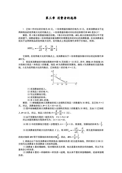
2. 假设某消费者的均衡如图教材中第96页的图3—22所示。
其中,横轴OX 1和纵轴OX 2分别表示商品1和商品2的数量,线段AB 为消费者的预算线,曲线U 为消费者的无差异曲线,E 点为效用最大化的均衡点。
已知商品1的价格P 1=2元。
(1)求消费者的收入; (2)求商品2的价格P 2; (3)写出预算线方程; (4)求预算线的斜率; (5)求E 点的MRS 12的值。
解答:(1)横轴截距表示消费者的收入全部购买商品1的数量为30单位,且已知P 1=2元,所以,消费者的收入M =2元×30=60元。
(2)图中纵轴截距表示消费者的收入全部购买商品2的数量为20单位,且由(1)已知收入M =60元,所以,商品2的价格P 2=M 20=6020=3(元)。
(3)由于预算线方程的一般形式为 P 1X 1+P 2X 2=M 所以本题预算线方程具体写为:2X 1+3X 2=60。
(4)将(3)中的预算线方程进一步整理为X 2=-23X 1+20。
很清楚,预算线的斜率为-23。
西方经济学第六版答案解析第三章消费者选择
第三章 消费者的选择1. 已知一件衬衫的价格为80元,一份肯德基快餐的价格为20元,在某消费者关于这两种商品的效用最大化的均衡点上,一份肯德基快餐对衬衫的边际替代率MRS 是多少? 解答:用X 表示肯德基快餐的份数;Y 表示衬衫的件数;MRS XY 表示在维持效用水平不变的前提下,消费者增加一份肯德基快餐消费时所需要放弃的衬衫的消费数量。
在该消费者实现关于这两种商品的效用最大化时,在均衡点上有边际替代率等于价格比,则有:201804X XY YP Y MRS X P ∆=-===∆它表明,在效用最大化的均衡点上,该消费者关于一份肯德基快餐对衬衫的边际替代率MRS 为。
2. 假设某消费者的均衡如图教材中第96页的图3—22所示。
其中,横轴OX 1和纵轴OX 2分别表示商品1和商品2的数量,线段AB 为消费者的预算线,曲线U 为消费者的无差异曲线,E 点为效用最大化的均衡点。
已知商品1的价格P 1=2元。
(1)求消费者的收入;(2)求商品2的价格P 2;(3)写出预算线方程;(4)求预算线的斜率;(5)求E 点的MRS 12的值。
解答:(1)横轴截距表示消费者的收入全部购买商品1的数量为30单位,且已知P 1=2元,所以,消费者的收入M =2元×30=60元。
(2)图中纵轴截距表示消费者的收入全部购买商品2的数量为20单位,且由(1)已知收入M =60元,所以,商品2的价格P 2=M 20=6020=3(元)。
(3)由于预算线方程的一般形式为 P 1X 1+P 2X 2=M所以本题预算线方程具体写为:2X 1+3X 2=60。
(4)将(3)中的预算线方程进一步整理为X 2=-23X 1+20。
很清楚,预算线的斜率为-23。
(5)在消费者效用最大化的均衡点E 上,有211212X P MRS X P ∆=-=∆,即无差异曲线斜率的绝对值即MRS 等于预算线斜率的绝对值P 1P 2。
因此,MRS 12=P 1P 2=23。
管理经济学 原书第六版 课后答案12

Chapter 12: Answers to Questions and Problems1.a. The expected value of option 1 is()()()()()300100161200164500166200164100161=++++. The expected value of option 2 is ()()()()()11111801701,0001708030055555++++=. b. The variance of option 1 is()()()()().000,2530010016130020016430050016630020016430010016122222=−+−+−+−+−Similarly, the variance of option 2 is 124,120. The standard deviation of option 1 is 158.11. The standard deviation of option 2 is 352.31.c. Option 2 is the most risky.2.a. Risk loving.b. Risk averse.c. Risk neutral.3.a.$5. b.She will purchase, since your price is less than her reservation price. c.$6. d. She will continue to search, since the price exceeds her reservation price.4.a. ()().6$100.4$200$140Ep =+=.b. Set Ep = MC to get 140 = 1 + 4Q . Solve for Q to find your profit-maximizing output, Q = 34.75 units.c. Your expected profits are (Ep)Q – C(Q) = $140(34.75) – (34.75 +2(34.75)2)=$2,415.13.5.a. The expected value, which is $25.b. The maximum value, which is $50.6.a. With only two bidders, n = 2. The lowest possible valuation is L = $1,000, and your own valuation is v = $2,500. Thus, your optimal sealed bid is$2,500$1,000$2,500$1,7502v L b v n −−=−=−=. b. With ten bidders, n =10. The lowest possible valuation is L = $1,000, and your own valuation is v = $2,500. Thus, your optimal sealed bid is$2,500$1,000$2,500$2,35010v L b v n −−=−=−=. c. With one hundred bidders, n =100. The lowest possible valuation is L = $1,000, and your own valuation is v = $2,500. Thus, your optimal sealed bid is$2,500$1,000$2,500$2,485100v L b v n −−=−=−=.7.a. With 5 bidders, n = 5. The lowest possible valuation is L = $50,000, and your own valuation is v = $75,000. Thus, your optimal sealed bid is$75,000$50,000$75,000$70,0005v L b v n −−=−=−=. b. A Dutch auction is strategically equivalent to a first-price sealed bid auction (see part (a)). Thus, you should let the auctioneer continue to lower the price until it reaches $70,000, and then yell “Mine!”c. $75,000, since it is a dominant strategy to bid your true valuation in a second-price, sealed-bid auction.d. Remain active until the price exceeds $75,000; then drop out.8.a. Hidden actions lead to moral hazard; hidden characteristics lead to adverse selection.b. Incentive contracts can solve moral hazard problems; screening and sorting can solve adverse selection problems.9. Since this is a common value auction, bidders will not bid their own private estimates because doing so would lead to the winner’s curse. Thus, there will be an additional incentive for bidders to shade their bids below their estimated valuations. The English auction format provides bidders the most information (therefore allowing them to pool information to some extent), mitigating this problem. For this reason, the English auction would generate the highest expected revenues in this case.10.Your expected inverse demand is E(P) = .5(200,000 – 250Q ) + .5(400,000 – 250Q ) = 300,000 – 250Q. Therefore, your expected marginal revenue is E(MR) = 300,000 – 500Q . Your marginal cost is MC = $200,000. Setting E(MR) = MC yields300,000500200,000Q −=. Solving, Q = 200. The price you expect is thus E(P) = 300,000 – 250(200) = $250,000. Your profits are thus ($250,000 -$200,000)(200) - $110,000 = $9,890,000.11. One would expect higher premiums on credit life, thanks to adverse selection. Peoplewho cannot pass physicals will select toward this type of insurance, resulting in higher premiums. Furthermore, people who are healthy and can pass a physical will be unwilling to pay the higher premiums, thus exacerbating this effect.12. The expected benefit from an additional search are 0.05($110,000 - $60,000) = $2,500, while the cost of another search is $5,000. Therefore, make her an offer. 13. In the absence of "guaranteed issue," an insurance company could choose to insure only those employees with a very low risk structure. In this case they offer lower rates because they experience fewer claims. But this leaves those workers with greater risk factors without insurance. By requiring insurers to offer coverage to all employees, the insurance company must take on employees that are less healthy and a greater risk. Why the controversy? By insuring those with greater health risks, the expected number of claims rises, thus increasing the cost of coverage. The workers with existing health problems benefit at the expense of healthy workers, who pay higher prices with "guaranteed issue." If the price rises high enough and healthy workers are free to drop coverage, this can result in adverse selection: The only people willing to pay the higher premiums are those in poor health.14. Brownstown Steel has better information about its financial situation than does its lenders, and is attempting to use this information advantage to enhance its bargaining position. If lenders gained full information about the financial situation of Brownstown Steel Corp., they would be in a position to squeeze the maximum amount from Brownstown Steel without fear of pushing it into bankruptcy. Absent the information, lenders will be more generous, since taking too much would increase the risk that Brownstown Steel goes bankrupt.15. The 30-day warranty and 10-point inspection. This not only reduces buyer risk from being duped by a used car dealer, but provides a costly signal about the quality of the used cars sold. An unscrupulous dealer would find it costly to mimic this strategy. Recognizing both of these facts, rational buyers will be more willing to purchase cars from the dealer.16. Offer two plans for customers with more than $1 million in assets. One plan (perhaps called the “Free Trade” Account) has an annual maintenance fee of $10,000 good for up to 400 “free” transactions (computed as $10,000/$25) per year (each additional transaction is priced at $25 each). The other plan (perhaps called the “Free Service” Account) has no annual maintenance fee but charges $100 per transaction. Given these two options, investors will sort themselves into the plans based on their individual characteristics.17.With 5 other bidders, n = 6. The lowest possible valuation is L = $5,000, and your own valuation is v = $12,000. Thus, your optimal first-price, sealed-bid is$12,000$5,000$12,000$10,833.336v L b v n −−=−=−=.18. A risk-neutral Oracle’s bid of $7 billion is low since the expected value of the presentvalue of the stream of profits is $7.6 billion. The public bidding process described most resembles an independent, private value English auction (each company places a different probability assessment on the value of the company that depends onpotential realized synergies). SAP’s expected value of the present value of the stream of profits is $8.4 billion. Since this is greater than Oracle’s expected value, SAP will win the “auction” and acquire PeopleSoft. SAP will pay just over $7.6 billion for PeopleSoft.19.The expected value of aggregate ten-year profits of a McDonald’s franchise is ()()()75.4$1$25.5$50.10$25.=−++million. Similarly, the expected value of a Penn Station East Coast Subs’ franchise is ()()75.4$)30$(025.5$95.30$025.=−++million. The variance and standard deviation of owning a McDonald’s franchise is()()()1875.1575.4125.75.4550.75.41025.2222'=−−+−+−=s McDonald σand 8971.31875.152''===s McDonald s McDonald σσ, respectively. Similarly, the variance and standard deviation for Penn Station East Coast Subs’ is()()()1875.4675.430025.75.4595.75.430025.2222=−−+−+−=Penn σand7961.61875.462===Penn Penn σσ, respectively. Since the expected values are thesame we can compare the standard deviations to determine the most risky investment. Since s McDonald Penn 'σσ>there is more risk associated with a Penn Station East Coast Subs’ franchise.20. There are several things for a student to consider in deciding to enroll in a traditionalMBA program or an online MBA program. It is likely that students with a spouse and family may be more attracted to online MBA programs, since these individuals are value stability and have others relying on them for income. In contrast, traditional MBA programs are more likely to attract singles who are willing to bear theopportunity cost associated with this form of education. Thus, there is an adverse selection issue. The individual who selects the traditional MBA program is likely to have a stronger signaling value regarding underlying characteristics.21.Market collapse is likely since “outsiders” will be unwilling to participate in equity (or other) markets since they know “insiders” will only sell a stock when they know the price is too high. Similarly, insiders will only buy when the price of a stock is known to be low. This is a losing proposition for outsiders, who would rationally choose not to participate in the market. This is an example of a moral hazard and is one of the primary reasons the SEC exists.。
《管理学》第六版周三多第三章思考题

《管理学》第六版周三多第三章思考题《管理学》第三章复习思考题1、什么是系统?系统有哪些基本特征?管理者可从系统原理中得到哪些启示?答:系统是指若干相互联系,相互作用的部分组成,在一定环境中具有特定功能的有机整体。
就其本质来说,系统是“过程的复合体”系统的特征:1)集合性。
这是系统最基本的特征。
一个系统至少由两个及两个以上的子系统构成。
2)层次性。
系统的结构是有层次的,构成一个系统的子系统和子子系统分别处于不同的地位3)相关性。
系统内各要素之间相互依存,相互制约的关系,就是系统的相关性;。
管理者可从系统原理中得到的启示:在实际工作中运用系统理论进行管理工作1:整体性原理,实际上就是从整体着眼,部分着手,统筹考虑,各方协调,达到整体的最优化2:动态性原理:运动是系统的生命,企业系统就是在不断变化的动态过程中生存和发展的,因此企业的产品结构、工艺过程,生产组织,管理机构,规章制度,经营方针,管理方法等都具有很强的时限性3:开放性原理:对外开放是系统的生命。
4:环境适应性原理:作为管理者既要有勇气看到能动的改变环境的可能,又要冷静地看到自己的局限,才能实事求是地作出科学的决策,保证组织的可持续发展5:综合性原理:管理者既要学会把许多普普通通的东西综合为新的构思、新的产品、创造出新的系统,又要善于把复杂的系统分解为最简单的单元去解决。
2、如何理解责任原理?责任原理的本质是什么?管理者可从责任原理中得到哪些启示?答:一、明确每个人的职责,挖掘人的潜能的最好的办法是明确每个人的职责1)职责的界限要清楚2)职责中要包括横向联系的内容3)职责一定要落实到每个人二、职位设计和权限委授要合理。
一定的人对所管的一定的工作是否能做到完全负责基本上取决于三个因素1)权限;实行任何管理都要借助于一定的权力。
2)利益;完全负责意味着责任者要承担全部风险,而任何的管理者在承担风险时,都自觉不自觉地要对风险和收益进行权衡,然后才决定是否值得去承担这种风险。
管理经济学 原书第六版 课后答案6
Chapter 6: Answers to Questions and Problems1.When an input has well-defined and measurable quality characteristics and requiresspecialized investments, the optimal procurement method is a contract. A contractreduces the likelihood of opportunistic behavior and underinvestment by creating alegal obligation between the firms. One disadvantage of a contract is that it increasesa firm’s transaction costs. An example, Boeing contracting with an aluminummanufacturer.2.When a firm requires a limited number of standardized inputs that are sold by manyfirms in the marketplace, the optimal method of procurement is spot exchange. Oneadvantage of spot exchange is that they permit firms to specialize. A disadvantage isthat the firm may potentially face the hold-up problem. An example, a painterpurchasing paint from a local paint store.3.a.Contract.b.Vertical Integration.c.Spot exchange (or possibly contract if a specific investment in many motors isrequired).d.Spot exchange.4.Engine manufacturing involves specific investments and a complex contractingenvironment. By vertically integrating, the potential for opportunism is reduced.Mirrors are relatively uniform products that can be purchased by spot exchange orcontract.5.a.Human capital.b.Physical asset specificity; note that the assembly line was designed especially fora particular firm’s product.c.Site specificity.6.The manager prefers the compensation scheme that pays a fixed salary plus apercentage of the profits. Essentially, the manager is faced with a choice between twoconsumption bundles: (1) a $125,000 fixed salary plus 10 hours of on-the-job leisureand (2) $125,000 in salary plus bonus plus 3 hours of on-the-job leisure. Since theoriginal compensation package of a $125,000 and 10 hours of shirking is stillavailable, the fact that she chose to work 7 hours reveals that she prefers the secondpay scheme.1 Managerial Economics and Business Strategy, 6e Page7.Spot checks and hidden video cameras are effective and relatively inexpensive toimplement initially. The disadvantage is that spot checks and hidden video camerasmay affect the morale of the workers. Moreover, implementing hidden camerasrequires more employees to monitor the cameras. The advantage of pay forperformance schemes is that it may be easier for a managers to observe individualworker (or group) performances. However, pay-for-performance schemes may becostly. In addition, when output is a function of group performance or its quality isdifficult to measure, an individual’s contribution to the output may not be observable. 8.a.Reduce the benefits of vertical integration.b.Reduce the benefits of vertical integration and lead firms to use contracts or spotexchange to procure inputs.c.Lead to contracts that are more detailed or vertical integration.d.Make spot exchange an unattractive method of procurement due to opportunismand possibly underinvestment.e.Make contracts a less attractive form of input acquisition.f.Lead to longer contracts, or in extreme instances, vertical integration.9.The environment in which computer manufacturers operate is very uncertain. The rateof technical progress among chip, and other hardware, manufacturers increases themarginal cost of signing long-term contracts.10. A contract decreases the problem of opportunism and still allows the firm tospecialize in production.11.Capping pension fund managers’ compensations would reduce the executives’incentives to maximize the value of the fund under their control, thereby reducing the overall return to the fund participants.12.Contracts requiring large specialized investments are expected to be longer thancontracts requiring relatively smaller specialized investments. The reason is thattransaction costs increase once the contract expires. By writing longer contracts, these costs can be avoided. Thus, large specialized investments increase the marginalbenefit of writing longer contracts.13.The first important point to make with shareholders is that restructuring the incentiveplan is designed to maximize shareholder value. This is achieved by givingemployees incentives to stay with the company longer, thereby reducing costlyemployee turnover and increasing the company’s profitability. Also, by restructuring the incentive plan, employees will want to find ways to work more productively andmake the company more profitable. The benefits to the shareholders and theemployees will be a higher stock price.14.The reduction in another supplier’s cost of producing airbags reduces GM’s marginalbenefit of contracting. Therefore, the 15-year contract that has been negotiated is too long; the optimal contract length is now less than 15 years.Page 2 Michael R. Baye15.The manager might pay a salesperson a base salary plus a percentage of the profits.This plan would penalize salespersons, to some extent, for excessive mileage.16.In the absence of an incentive contract, a manager may still choose to maximizeprofits in order to build a reputation in being a superb manager and increasing thepotential of future management opportunities. Furthermore, the threat of a takeoverby other investors and job loss also disciplines managers to maximize profits, even ifthey are paid a fixed salary.17.No.18.The principal-agent problem in this situation exists between on-duty police officers(the agent) and the city officials who hire them (the principals). On-duty policeofficers were supposed to prevent picket lines from blocking worker access. Membersof the police union appear to be engaging in opportunistic behavior to improve theirbargaining power. The city of Boston has committed to spending $14 million to hostthe DNC and the police union is attempting to take advantage of this specializedinvestment. Therefore, the city of Boston is facing the “hold-up problem” as definedin the book. The problem also illustrates the problem of writing contracts: when thecity of Boston wrote a contract with Shawmut Design and Construction there weremany unforeseeable events that may not explicitly be defined in the contract.19.Business-process outsourcing (BPO) is a contractual relationship with a third-partyfirm, whereas a firm that produces human resource services internally is verticallyintegrated. Contracting human resource services with a third party allows the firm tospecialize in activities related to its core business, which as the problem points outmay result in large cost savings. Contracts, however, are costly to write and oftenincomplete. These reasons provide justification for vertical integration. Contractingwith an international-based firm may be more costly since the contract must bewritten in a manner to protect the firm in a foreign country. This extra cost should becompared to the extra benefit (cost savings) that accrues from lower off shore labor.Furthermore, there may be cultural difference in hiring practices that may makeoutsourcing from human resources to an international firm less attractive.20.If partners in the law firm are paid an equal share of the overall profits of the firm,regardless of how much they contribute, lawyers nearing retirement will have anincentive to stay with the firm while doing as little work as possible. In this way, heor she can enjoy “semi-retirement,” but will continue to earn a share of the profitsfrom other’s hard work. For this reason, most law firms have mandatory retirement tomitigate incentive compatibility problems. Eliminating mandatory retirement isprobably not a good idea for your 30-year old client.21.The money the dealership pays to train workers in the form of time and expenses is aspecialized investment in human capital. The investment only has value to thedealership if workers remain with the dealership and the dealership maintains itsrelationship ADP. Once this is sunk, it faces a potential “hold-up” problem fromworkers and ADP: If either party decides to sever the relationship, the dealership willhave to sink additional funds into training new employees.3 Managerial Economics and Business Strategy, 6e Page。
(NEW)曼昆《经济学原理(微观经济学分册)》(第6版)课后习题详解
目 录第1篇 导 言第1章 经济学十大原理第2章 像经济学家一样思考第3章 相互依存性与贸易的好处第2篇 市场如何运行第4章 供给与需求的市场力量第5章 弹性及其应用第6章 供给、需求与政府政策第3篇 市场和福利第7章 消费者、生产者与市场效率第8章 应用:赋税的代价第9章 应用:国际贸易第4篇 公共部门经济学第10章 外部性第11章 公共物品和公共资源第12章 税制的设计第5篇 企业行为与产业组织第13章 生产成本第14章 竞争市场上的企业第15章 垄 断第16章 垄断竞争第17章 寡 头第6篇 劳动市场经济学第18章 生产要素市场第19章 收入与歧视第20章 收入不平等与贫困第7篇 深入研究的论题第21章 消费者选择理论第22章 微观经济学前沿第1篇 导 言第1章 经济学十大原理一、概念题1.稀缺性(scarcity)答:经济学研究的问题和经济物品都是以稀缺性为前提的。
稀缺性指在给定的时间内,相对于人的需求而言,经济资源的供给总是不足的,也就是资源的有用性与有限性。
人类消费各种物品的欲望是无限的,满足这种欲望的物品,有的可以不付出任何代价而随意取得,称之为自由物品,如阳光和空气;但绝大多数物品是不能自由取用的,因为世界上的资源(包括物质资源和人力资源)是有限的,这种有限的、为获取它必须付出某种代价的物品,称为“经济物品”。
正因为稀缺性的客观存在,地球上就存在着资源的有限性和人类的欲望与需求的无限性之间的矛盾。
经济学的一个重要研究任务就是:“研究人们如何进行抉择,以便使用稀缺的或有限的生产性资源(土地、劳动、资本品如机器、技术知识)来生产各种商品,并把它们分配给不同的社会成员进行消费。
”也就是从经济学角度来研究使用有限的资源来生产什么、如何生产和为谁生产的问题。
2.经济学(economics)答:经济学是研究如何将稀缺的资源有效地配置给相互竞争的用途,以使人类的欲望得到最大限度满足的科学。
时下经常见诸国内报刊文献的“现代西方经济学”一词,大多也都在这个意义上使用。
管理经济学原书第六版课后答案10
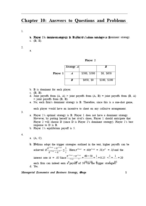
Managerial Economics and Business Strategy, 6e Page 1 Chapter 10: Answers to Questions and Problems 1.a. Player 1’s dominant strategy is B. Player 2 does not have a dominant strategy. b.Player 1’s secure strategy is B. Player 2’s secure strategy is E. c. (B, E). 2. a. b. B is dominant for each player. c. (B, B). d. Joint payoffs from (A, A) > joint payoffs from (A, B) = joint payoffs from (B, A) > joint payoffs from (B, B). e. No; each firm’s dominant strategy is B. Therefore, since this is a one-shot game, each player would have an incentive to cheat on any collusive arrangement. 3.a. Player 1’s optimal strategy is B. Player 1 does not have a dominant strategy. However, by putting herself in her rival’s shoes, Player 1 should anticipate that Player 2 will choose D (since D is Player 2’s dominant strategy). Player 1’s best response to D is B. b. Player 1’s equilibrium payoff is 5. 4.a. (A, C). b.No. c.If firms adopt the trigger strategies outlined in the text, higher payoffs can be achieved if 1.Cheat Coop Coop Ni ππππ−≤− Here, πCheat = 60, πCoop = 50, πN = 10, and the , and the interest rate is i = .05. Since . Since 605010.2550104Cheat Coop Coop Nππππ−−===−− < 1120.05i == each firm can indeed earn a payoff of 50 via the trigger strategies. d. Yes. Player 2 Strategy A B A $500, $500 $0, $650 Player 1 B $650, $0 $100, $100 ($0, $15)RightRightLeftLeft 12($200, $300)Not IntroducePrice WarIntroduceKmartStrategy Sale Price Regular Price Sale Price$1, 1 $5, $3Regular Price $3, $5 $3, $3Ford Strategy Airbags No No Airbags Airbags Airbags $1.5, 1.5 $2,-$1 No Airbags -$1, $2 $0.5, $0.5 PCRival Advertise No Yes No $8, $8 -$1, $48Kellogg’sYes$48,-$1$0, $0strategies if ππRival Strategy: Price Low High Low $0, $0 $9,-$1 High -$1, $9 $7, $7BakerPrice $10 $20$5 15, 16 15,18 Argyle$10 10, 16 10,18NetWorksStrategy 250 Units 500 Units250 Units $12500, $12500 $7500, $15000500 Units $15000, $7500 $10000, $1000018.The normal-form representation of this game is depicted in the following payoffmatrix.T-MobileStrategies CDMA GSMCDMA $16 b, $12 b $12 b, $8 bQualcommGSM $14 b, $7 b $13 b, $18 bThere are two Nash equilibria to this coordination game: (1) Qualcomm and T-Mobile adopt the CDMA technology and (2) Qualcomm and T-Mobile adopt theGSM technology. There are many ways to solve multiplicity of equilibria in thiscoordination problem. As the book points out, the firms could “talk” to each andagree on one technology. Alternatively, Iraq’s government could announce whichtechnology is to be used in the country.19.The normal form of this game is contained in the following payoff matrix (in billionsof U.S. dollars).JapanStrategies Tariff No TariffTariff $43.78, $4.76 $44.2, $4.66U.S.No tariff $43.66, $4.85 $44, $4.8The Nash equilibrium is for the U.S. and Japan to each impose tariffs. However, both countries achieve greater welfare by “agreeing” to impose no tariffs. Thesustainability of such an agreement to impose no tariffs is dependent upon the game being repeated infinitely, the countries using trigger strategies and the interest ratebeing sufficiently low.20.You should not recommend that the office manager invest more time monitoring. Theproblem is not that she is monitoring too little. Rather, her monitoring activities and strategies are predictable. Workers realize that once she leaves after the 9 a.m. check, she is unlikely to return until 11 a.m. Recognizing this, workers know they will not get caught “goofing off” (shirking). The manager best strategy is to randomize boththe timing and number of checks she does each day. That way, her monitoring is not predictable and workers will respond by spending less time shirking.Page 6 Michael R. Baye。
管理经济学原书第六版课后题答案,第二章答案
Chapter 2: Answers to Questions and Problems1.a. Since X is a normal good, an increase in income will lead to an increase in the demand for X (the demand curve for X will shift to the right).b. Since Y is an inferior good, a decrease in income will lead to an increase in the demand for good Y (the demand curve for Y will shift to the right).c. Since goods X and Y are substitutes, a decrease in the price of good Y will lead to a decrease in the demand for good X (the demand curve for X will shift to the left).d. No. The term “inferior good” does not mean “inferior quality,” it simply means that income and consumption are inversely related.2.a. The supply of good X will decrease (shift to the left).b. The supply of good X will decrease. More specifically, the supply curve will shift vertically up by exactly $1 at each level of output.c. The supply of good X will decrease. More specifically, the supply curve will rotate counter-clockwise.d. The supply curve for good X will increase (shift to the right).3.a. ()()500.550053050s x Q =−+−= units.b. Notice that although ()()500.550530175s x Q =−+−=−, negative output isimpossible. Thus, quantity supplied is zero.c. To find the supply function, insert 30z P = into the supply equation to obtain()500.55302000.5s x x x Q P P =−+−=−+. Thus, the supply equation is2000.5s x x Q P =−+. To obtain the inverse supply equation, simply solve thisequation for x P to obtain 4002s x x P Q =+. The inverse supply function is graphedin Figure 2-1.$0.0$200.0$400.0$600.0$800.0$1,000.0$1,200.0$1,400.0$1,600.00100200300400500Quantity of X Price of XSFigure 2-1a. Good Y is a substitute for X, while good Z is a complement for X.b. X is a normal good.c. ()()()()000,5000,55$10190$8900,5$41910,4$21200,1=+−+−=d x Q d. For the given income and prices of other goods, the demand function for good X is ()()()1111,200$5,9008$90$55,000,2410d x x Q P =−+−+ which simplifies to 7,4550.5d x x Q P =−. To find the inverse demand equation, solve for price to obtain 14,9102.d x x P Q =− The demand function is graphed in Figure 2-2.$0$2,982$5,964$8,946$11,928$14,910010002000300040005000600070008000Quantity of X Price of XDemandFigure 2-25.a. Solve the demand function for x P to obtain the following inverse demand function: 11154d x x P Q =−. b. Notice that when $35x P =, ()460435320d x Q =−= units. Also, from part a, weknow the vertical intercept of the inverse demand equation is 115. Thus,consumer surplus is $12,800 (computed as ()().5$115$35320$12,800−=). c. When price decreases to $25, quantity demanded increases to 360 units, so consumer surplus increases to $16,200 (computed as()().5$115$25360$16,200−=).d. So long as the law of demand holds, a decrease in price leads to an increase in consumer surplus, and vice versa. In general, there is an inverse relationship between the price of a product and consumer surplus.a. Equating quantity supplied and quantity demanded yields the equation150102P P −=−. Solving for P yields the equilibrium price of $40 per unit. Plugging this into the demand equation yields the equilibrium quanity of 10 units (since quantity demanded at the equilibrium price is ()504010d Q =−=). b. A price floor of $42 is effective since it is above the equilibrium price of $40. As a result, quantity demanded will fall to 8 units ()84250=−=d Q , while quantity supplied will increase to 11 units ()⎟⎠⎞⎜⎝⎛=−=11104221s Q . That is, firms produce 11 units but consumers are willing and able to purchase only 8 units. Therefore, at a price floor of $42, 8 units will be exchanged. Since s d Q Q <there is a surplus amounting to 3811=−units.c. A price ceiling of $30 per unit is effective since it is below the equilibrium price of $40 per unit. As a result, quantity demanded will increase to 20 units ()203050=−=d Q , while quantity supplied will decrease to 5 units()⎟⎠⎞⎜⎝⎛=−=5103021s Q . That is, while firms are willing to produce only 5 units consumers want to buy 20 units at the ceiling price. Therefore, at the price ceiling of $30, only 5 units will be available to purchase. Since s d Q Q >, there is a shortage amounting to 15520=− units. Since only 5 units are available at a price of $30, the full economic price is the price such that quantity demanded equals the 5 available units: 550F P =−. Solving yields the full economic price of $45.7.a. The shortage is 3 units (since at a price of $6, 413d s Q Q −=−= units). The full economic price is $12.b. The surplus is 1.5 units (since at a price of $12, 2.51 1.5s d Q Q −=−= units. The cost to the government is $18 (computed as ($12)(1.5) = $18).c. The excise tax shifts supply vertically by $6. Thus, the new supply curve is 1S and the equilibrium price increases to $12. The price paid by consumers is $12 per unit, while the amount received by producers is this $12 minus the per unit tax. Thus, producers receive $6 per unit. After the tax, the equilibrium quantity sold is 1 unit.d. At the equilibrium price of $10, consumer surplus is ().5$14$102$4−=. Producer surplus is ().5$10$22$8−=.e. No. At a price of $2 no output is produced.a. Equate quantity demanded and quantity supplied to obtain 1117242x x P P −=−. Solve this equation for x P to obtain the equilibrium price of 10x P =. Theequilibrium quantity is 2 units (since at the equilibrium price quantity demanded is ()171022d Q =−=). The equilibrium is shown in Figure 2-3.$0$2$4$6$8$10$12$14$16$18$200123456Quantity of XPrice of XDemandFigure 2-3b. A $6 excise tax shifts the supply curve up by the amount of the tax.Mathematically, this means that the intercept of the inverse supply function increases by $6. Before the tax, the inverse supply function is S Q P 42+=. After the tax the inverse supply function is 84s P Q =+, and the after tax supplyfunction (obtained by solving for s Q in terms of P) is given by 124s Q P =−. Equating quantity demanded to after-tax quantity supplied yields117224P P −=−. Solving for P yields the new equilibrium price of $12. Plugging this into the demand equation yields the new equilibrium quantity, which is 1 unit.c. Since only one unit is sold after the tax and the tax rate is $6 per unit, total tax revenue is only $6.9. A technological breakthrough that reduces production costs will lead to a rightwardshift in the supply curve for RAM chips, resulting in a lower equilibrium price of RAM chips. If in addition, income increases, the demand for RAM chips will also increase since they are a normal good. This increase in demand would tend to increase the price of RAM chips. The ultimate effect of both of these changes in supply and demand on the equilibrium price of RAM chips is indeterminate.Depending on the relative magnitude of the increase in supply and demand, the price you will pay for chips may rise or fall.10. The tariff reduces the supply of raw sugar, resulting in a higher equilibrium price of sugar. Since sugar is an input in making generic soft drinks, this increase in input prices will decrease the supply of generic soft drinks (putting upward pressure on the price of generic soft drinks and tend to reduce quantity). Coke and Pepsi’s advertising campaign will decrease the demand for generic soft drinks (putting downward pressure on the price of generic soft drinks and further reducing the quantity). For these reasons, the equilibrium quantity of generic soft drinks sold will decrease.However, the equilibrium price may rise or fall, depending on the relative magnitude of the shifts in demand and supply.11. No. this confuses a change in demand with a change in quantity demanded. Higher cigarette prices will not reduce (shift to the left) the demand for cigarettes.12.To find the equilibrium price and quantity, equate quantity demanded and quantity supplied to obtain 1752200P P −=−. Solving yields the new equilibrium price of $125 per pint. The equilibrium quantity is 50 units (since 17512550d Q =−= units at that price). Consumer surplus is ()250,1$50125$175$21=×−. Producer surplus is ()625$50100$125$21=×−. See Figure 2-4.$0.0$25.0$50.0$75.0$100.0$125.0$150.0$175.0$200.00102030405060Quantity Price Demand SupplyFigure 2-413. This decline represents a leftward shift in the supply curve for oil, and will result inan increase in the equilibrium price of crude oil. Since oil is an input in producing gasoline, this will decrease the supply of gasoline, resulting in a higher equilibrium price of gasoline and a lower equilibrium quantity. Furthermore, the higher price of gasoline will increase the demand for substitutes, such as small cars. The equilibrium price of small cars is likely to increase, as is the equilibrium quantity of small cars. 14. Equating the initial quantity demanded and quantity supplied gives the equation: 25054110P P −=−. Solving for price, we see that the initial equilibrium price is $40 per month. When the tax rate is reduced, equilibrium is determined by the following equation: 2505 4.171110P P −=−. Solving, we see that the newequilibrium price is about $39.25 per month. In other words, a typical subscriber would save about 75 cents (the difference between $40.00 and $39.25).15. Dry beans and rice are probably inferior goods. If so, an increase in income shifts demand for these goods to the left, resulting in a lower equilibrium price. Therefore, G.R. Dry Foods will likely have to sell its products at a lower price.16.Figure 2-5 illustrates the relevant situation. The equilibrium price is $2.75, but the ceiling price is $0.75. Notice that, given the shortage of 12 million transactions caused by the ceiling price of $0.75, the average consumer spends an extra 12minutes traveling to another ATM machine. Since the opportunity cost of time is $20 per hour, the non-pecuniary price of an ATM transaction is $4 (the $20 per hour wage times the fractional hour, 12/60, spent searching for another machine). Thus, the full economic price under the price ceiling is $4.75 per transaction.Quantity (Millions of Transactions)ATM Fee$4.75$0.75Figure 2-517. The unusually cold temperatures have caused a decrease in the supply of grapes usedto produce Chilean wine, resulting in higher prices. These grapes are an input in making wine, so the supply of Chilean wine decreases and its price increases. Since California and Chilean wines are substitutes, an increase in the price of Chilean wine will increase the demand for Californian wines causing an increase in both the price and quantity of Californian wines.18.Substituting 940=desktop P into the demand equation yields memory d memory P Q 809060−=. Similarly, substituting 100=N into the supply equationyields memory S memory P Q 201100+=. The competitive equilibrium level of industry outputand price occurs where S memoryd memory Q Q =, which occurs when industry output 2692*=memory Q (in thousands) and the market price is 60.79$*=memory P per unit. Since 100 competitors are assumed to equally share the market, Viking should produce26.92 thousand units. If 1040$=desktop P , memory d memory P Q 808960−=. Under thiscondition, the new competitive equilibrium occurs when industry output is 2672 thousand units and the per-unit market price is $78.60. Therefore, Viking should produce 26.72 thousand units. Since demand decreased (shifted left) when the price of desktops increased, memory modules and desktops are complements.19. Mid Towne IGA aimed to educate consumers that its contract with Local 655 unionmembers was different than its rivals, so it engaged in informative advertising. Mid Towne IGA’s informative advertising increases demand (demand shifts rightward) resulting from (1) Local 655 union members locked out of rival supermarkets (2) consumers who are sympathetic to the Local 655 union, and (3) consumers who do not like the aggravation of picketing employees and other disruptions at thesupermarket. This shift is depicted in Figure 2-6, where the equilibrium price and quantity both increase. It is unlikely that demand will remain high for Mid Towne IGA. As contracts are renegotiated and Local 655 union members are back to work, demand will likely settle back around its original level.Figure 2-6 20. The price gouging statute imposes an effective price ceiling on necessarycommodities during times of emergencies; legally retailers cannot raise prices by a significant amount. When a natural disaster occurs, the demand for necessarycommodities such as food and water can dramatically increase, as people want to be stocked-up on emergency items. In addition, since it can be difficult for retailers to receive shipments during emergency periods, the supply of these items is often reduced. Given the simultaneous reduction in supply and increase in demand, one would expect the price to increase during times of emergencies. However, since the price gouging statute acts as a price ceiling, the price will probably remain at its normal level, and a shortage will result. Quantity212P 1P 221.While there is undoubtedly a link between unemployment and crime, the governor’splan is likely flawed since it only examines one side of the market. Raising theminimum wage will make the prospect of working more appealing for teenagers, but it will also have an effect on business owners and managers in the state. Theminimum wage is a price floor. Raising the minimum wage will reduce the quantity demand for labor within the state, and result in a labor surplus. More teenagers will seek jobs, but fewer businesses will hire teenagers. In all likelihood, the governor’s plan will result in greater juvenile delinquency.。
(NEW)曼昆《经济学原理(微观经济学分册)》(第6版)课后习题详解
目 录第1篇 导 言第1章 经济学十大原理第2章 像经济学家一样思考第3章 相互依存性与贸易的好处第2篇 市场如何运行第4章 供给与需求的市场力量第5章 弹性及其应用第6章 供给、需求与政府政策第3篇 市场和福利第7章 消费者、生产者与市场效率第8章 应用:赋税的代价第9章 应用:国际贸易第4篇 公共部门经济学第10章 外部性第11章 公共物品和公共资源第12章 税制的设计第5篇 企业行为与产业组织第13章 生产成本第14章 竞争市场上的企业第15章 垄 断第16章 垄断竞争第17章 寡 头第6篇 劳动市场经济学第18章 生产要素市场第19章 收入与歧视第20章 收入不平等与贫困第7篇 深入研究的论题第21章 消费者选择理论第22章 微观经济学前沿第1篇 导 言第1章 经济学十大原理一、概念题1.稀缺性(scarcity)答:经济学研究的问题和经济物品都是以稀缺性为前提的。
稀缺性指在给定的时间内,相对于人的需求而言,经济资源的供给总是不足的,也就是资源的有用性与有限性。
人类消费各种物品的欲望是无限的,满足这种欲望的物品,有的可以不付出任何代价而随意取得,称之为自由物品,如阳光和空气;但绝大多数物品是不能自由取用的,因为世界上的资源(包括物质资源和人力资源)是有限的,这种有限的、为获取它必须付出某种代价的物品,称为“经济物品”。
正因为稀缺性的客观存在,地球上就存在着资源的有限性和人类的欲望与需求的无限性之间的矛盾。
经济学的一个重要研究任务就是:“研究人们如何进行抉择,以便使用稀缺的或有限的生产性资源(土地、劳动、资本品如机器、技术知识)来生产各种商品,并把它们分配给不同的社会成员进行消费。
”也就是从经济学角度来研究使用有限的资源来生产什么、如何生产和为谁生产的问题。
2.经济学(economics)答:经济学是研究如何将稀缺的资源有效地配置给相互竞争的用途,以使人类的欲望得到最大限度满足的科学。
时下经常见诸国内报刊文献的“现代西方经济学”一词,大多也都在这个意义上使用。
经济学原理第六版课后答案

经济学原理第六版课后答案第一章,经济学原理和经济行为。
1. 什么是经济学?经济学是研究人们如何利用稀缺资源来生产、分配和消费商品和服务的社会科学。
2. 经济学家如何对待假设?经济学家会做出一些简化的假设,以便更好地分析经济现象。
这些假设可以帮助经济学家建立模型,从而更好地理解和解释现实世界中的经济问题。
3. 什么是机会成本?机会成本是指为了得到某种东西所放弃的东西的价值。
在资源有限的情况下,做出某种选择意味着放弃其他选择,因此机会成本是每个选择的代价。
4. 什么是边际分析?边际分析是指对一种行为或决策的边际变化进行分析。
经济学家通过比较边际成本和边际收益来做出决策。
5. 什么是正面分析和规范分析?正面分析是描述经济现象的方式,而规范分析则是对经济现象进行评价和给出建议的方式。
第二章,供求和市场均衡。
1. 什么是市场?市场是买卖商品和服务的地方,也可以是指交易双方的总体。
2. 什么是需求曲线?需求曲线表示了消费者在不同价格水平下愿意购买的商品数量。
需求曲线通常是向下倾斜的,这意味着价格上涨时需求量下降,价格下跌时需求量增加。
3. 什么是供给曲线?供给曲线表示了生产者在不同价格水平下愿意提供的商品数量。
供给曲线通常是向上倾斜的,这意味着价格上涨时供给量增加,价格下跌时供给量减少。
4. 市场均衡是如何确定的?市场均衡是指供给和需求达到平衡的状态,此时市场上的商品数量和价格达到了最优的状态。
市场均衡的价格和数量由供给曲线和需求曲线的交点确定。
5. 什么是价格弹性?价格弹性是指需求量或供给量对价格变化的敏感程度。
如果需求量或供给量对价格变化非常敏感,那么价格弹性就会很大;反之则会很小。
第三章,边际效用和边际成本。
1. 什么是边际效用?边际效用是指消费一个额外单位商品或服务所带来的额外满足程度。
通常情况下,随着消费数量的增加,边际效用会递减。
2. 什么是边际成本?边际成本是指生产一个额外单位商品或服务所需要的额外成本。
管理经济学课后练习部分参考答案
第1章 导论选择题:1-5:ABBCD 6:C第二章 供求分析选择题:1-5:ACCBD 6-8:CCA第三章 消费者效用分析选择题:1-5:DCABC 6-10:BBCAD 11-13:CAD计算题:3. 假定某人只能买到两种商品,他的年收入为10000元,牛肉的价格为每千克9元,土豆的价格为每千克2元。
(1)如果把牛肉的购买量当作因变量,请写出预算约束线的方程。
(2)(3)5. 消费者每周花360元买X、Y两种商品。
其中PX=3元,PY=2元,它的效用函数为U=2X2Y ,在均衡状态下,他每周买X、Y各多少?解:6043,804323360,2336043,2234,2,422===∴⨯+=∴+==∴======X Y X X X Y X X Y X XY P MU P MU X dYdU MU XY dX dU MU Y X X Y X 得:又6.某人的收入是12元/天,并把每天的收入花在X 、Y 两种商品上。
他的效用函数为U=XY 。
X 的价格为每单位2元,Y 的价格为每单位3元。
问:①他每天买X.Y 各多少才能使他的效用最大?6232,3323212,321232,32,,==∴===∴⨯+=+==∴======XY U X Y X X X Y X X Y X Y P MU P MU X dYdU MU Y dX dU MU Y Y X X Y X 又②如果X 的价格上涨44%,Y 的价格不变,他的收入必须增加多少才能维持他起初的效用水平?元。
入要增加要维持原有的效用,收效用不变, 2.44.2124.144.144.235.288.24.2388.2,5.2388.26,388.266388.2,388.2,88.22%)441(2∴=-=∆=⨯+⨯=+=∴===∴=⨯=∴==∴===⨯+=I Y P X P I X Y X X X X XYX Y X Y P MU P MU Y X Y Y X X X第4章 需求弹性与供给弹性选择题:1-5:C(BDA)DAA 6-8:BAB 第9题题干有问题,如果改为供给价格弹性则选AD计算题:1.某商场将服装A 的价格由120元打6折促销,结果该服装的日销量由先前的12件升至30件,据此计算:①该服装的需求价格弹性。
管理经济学课后答案

第一章:P201.若某彩电市场上,市场的供给函数和需求函数分别为Qs = -450000 200PQd =450000-100PQs和Qd分别为供给和需求的数量,单位是台;P为市场价格,单位是元/台。
求市场上彩电的均衡价格和成交数量。
若人们的收入增加,需求函数为Qd=510000-100P这时市场上均衡的价格和交易量又有什么变化?Qd 二Qs答.450000 -100P 二-450000 二200P口,P= 3000Q 二150000此时彩电的均衡价格为3000元,均衡数量为150000台。
Qd =Qs510000-100P =-450000 200PP =3200Q =190000此时均衡价格为3200元,均衡数量为190000台,相比之前均衡价格增加200元,均衡数量增加40000台。
第二章:49页1.某空调生产商认为其一品牌的空调机在某市场上的需求曲线如下:P=6 000-5Q 式中,P为每台空调机的价格(元/台);Q为每月在该市场上的销量(台)。
要想每月能在该市场上销售400台,应当定什么价格?如果价格定在3 600元,能销售多少台?在价格为3 200元/台时,需要价格弹性是多少?会在需求单一价格弹性时出售空调机吗?(1)每月在市场上销售400台,即此时Q=400由题意可知,P =6000 —5Q =6000 —5 400 = 4000 (元/ 台)1(2)由P =6000-5Q= Q =1200 P ,5价格定在3600,即此时P =3600二Q =1200—」3600 = 480 (台) 5 (3)由题意可知,价格P = 3200时,可以求出Q=560需求价格弹性二垃P「偉也一8dP Q 5 560 7(4)需求单一弹性表示此时的需求价格弹性为1,由需求价格弹性公式可知1 =丄P=P=5Q,5 Q又P = 6000 - 5Q 二P 二3000,Q 二600总收益二PQ = 6000Q - 5Q2对总收益求一阶导数并令其等于0 ,即6000 - 10Q = 0,刚好求得Q =600,并且总收益的二阶导数为-10,是最大值点,因此,会在需求单一价格弹性时出售空调机。
管理经济学 原书第六版 课后答案13
Chapter 13: Answers to Questions and Problems1.a. 16 units.b. Note that P = $200, AC = $180, and Q = 16, so profits are ($200 - $180)(16) = $320.c. Yes; if it can credibly commit to a higher output it will earn even greater profits. 2.a. $10$40$90.2D MD M i ππΠ=+=+= million. b. ()21111.2...$8$4811.2L L L L L i i i i ππππ++⎛⎞⎛⎞⎛⎞Π=+++===⎜⎟⎜⎟⎜⎟++⎝⎠⎝⎠⎝⎠million. Since this is less than the profits obtained if entry occurs, the firm should notengage in limit pricing.3.a. The simultaneous-move equilibrium is (Yes, Yes), and Player 1 earns $200 in this equilibrium. By going first player 1’s best strategy is to commit to “No.” Player2’s best response would be “No”, and thus Player 1 would earn $350 by goingfirst. The maximum amount Player 1 should pay for going first is this $150 (orperhaps $149.99). Importantly, this assumes Player 1’s move is observed byPlayer 2 before Player 2 makes her decision.b. Player 2 gets $200 when Player 1 goes first, compared to $225 when they move at the same time. Thus, player 2 would be willing to pay up to $25 to keep player 1 from moving first.4.a. A network with 10 users provides 10(10 - 1) = 90 potential connection services.b. No. Revenues will be $1,000 which is well short of the $6,000 in costs.c. Yes. With 90 connection services, each consumer will pay $900 to join thenetwork. Since there are 10 consumers, total revenues are $9,000. This exceedsthe $6,000 required to build the network.d. The number of potential connection services increases by 20 to 110.5.a. Two examples include tactics that raise distribution costs or increase the price of inputs.b. No. The benefits stem from the fact that by raising rivals’ costs, your rivals reduce their own output. This tends to increase the market price, thus permitting you toexpand your own output (and market share) to enjoy higher profits.6.a.Firm 2 will enter so Firm 1 earns profits of $300 thousand.b.By eliminating the fee, Firm 2 still has an incentive to enter. Firm 1 earns profitsof $340 thousand.c.The $300 thousand increase in the medallion fee eliminates Firm 2’s incentive toenter (since its profits are -$100 thousand upon entry). Since Firm 2 does notenter, Firm 1 earns profits of $400 thousand.d.The optimal change is an increase of $200 thousand (or perhaps $200 thousandplus one cent). This makes it unprofitable for Firm 2 to enter. Firm 1 earns profitsof $500 thousand.e.Yes; the city gets a higher fee which is probably good politically.7.a.Since last year’s market price was $8, it follows that Firm 1 produced 1 millionunits last year (since P = 10 – 2Q = 8 implies Q = 1 million). For this to be theprofit-maximizing price (MR = MC), it follows that 10 – 4Q = MC. Since Q = 1,Firm 1’s marginal cost was $6 last year – the same as Firm 2’s marginal cost thisyear. Thus, it would appear that Firm 1’s marginal cost has declined over time dueperhaps to learning curve effects.b.At the current market price of $8, total market output is 1 million. Thus, each firmsells 0.5 million units. Each firm’s fixed costs are $1 million. Firm 1’s profits arethus ($8 - $2)(.5) - $1 = $2 million and Firm 2’s profits are ($8 - $6)(.5) - $1 = $0million.c.Firm 1’s profits would increase to ($6 - $2)(2) - $1 = $7 million and Firm 2’sprofits would fall to -$1 million.d.No; $6 is the monopoly price.e.No; it is not pricing below its own marginal cost.8.Your best strategy is to preempt them by committing to target households before theyhave a chance to commit to target professionals. If you can credibly and publiclycommit to your strategy before they commit to their strategy, their best response will be to target households. You will earn $100 million and ultimately drive them out of the market.9.Penetration pricing (see the text for details).10.This pattern of pricing is consistent with predatory pricing, which is illegal under theSherman Antitrust Act. However, it is not illegal to lower prices to meet competition, so the observed pricing is also consistent with competitive behavior. It is oftendifficult to establish that a firm priced below marginal cost. For the case of an airline, this is even more problematic. At one extreme, one might argue that the marginal cost of putting one more passenger on an existing flight is zero. At the other extreme, one might argue that it is the marginal cost of adding another flight rather than anotherpassenger that is relevant.11.No. Profits are negative from limit pricing, but strictly positive otherwise. Regardlessof the interest rate and the timing of profit flows (at the start or the end of eachperiod), Palm would earn less by limit pricing than by permitting entry.12.Not necessarily. Due to network effects, penetration pricing was probably optimal formany companies. To the extent that there is consumer lock-in, the number of hitscould be a good proxy for the long-run profitability of a site once a firm begins toincrease prices above the penetration pricing level. Ultimately, however, hits musttranslate into profits in order for such companies to survive.13.As shown in the text, strategies that raise the cost of potential entrants – even whendoing so raises the costs of incumbents – can lead to less entry and higher profits for incumbents. To the extent that such practices raise costs, they may be motivated outof self-interest (to limit entry) rather than a concern about social welfare.14.First, note that the monopoly price is P = $210, the monopoly output is Q =1,666,666.67, and monopoly profits are $16,666,667. (To see this, note that =− and MC = $200, so setting MR = MC and solving yields these220.000012MR Qresults). Second, notice that with the subsidy the firm’s average cost curve is constant at $200 per unit. Thus, to prevent entry via limit pricing, Barnacle would have toprice its product at $200. Doing so would yield zero profits. A better strategy forBarnacle is to lobby to eliminate the $9 million in subsidies while committing toproduce its current (monopoly) level of output. This would reduce Barnacle’s profits to $7.67 million per year, but would make it unprofitable for an entrant to enter themarket.15.Such a premium might be justified when there are significant network externalities. Inthis case, adding one more customer to a network of n customers increases thenumber of potential network connections by 2n. To the extent that a brokeragecompany is a two-way network that benefits from having a network of customers that can be matched as buyers and sellers, there is a potential business rationale. Whether this justifies a premium of $100 per customer is an entirely different matter andsubject to some debate.16.Notice that Argyle earns profits from both the sale of wool and sweaters. To theextent that overall profits are enhanced by selling both, it is rational to do so.However, if selling wool to other downstream suppliers reduces its overall profits, it may be able to increase its profits by raising rivals’ costs, a vertical price squeeze, or vertical foreclosure.17.Unfortunately, your best option is to accept the offer. If you don’t, your rival willpurchase the machine. If you purchase the machine, your profits are $15 - $24 = -$9million. This is better than the -$10 million you will earn if your rival has anopportunity to buy the machine.18.Each bank can be viewed as a star network: the bank is the hub and ATMs areconsumer access points. An agreement that expands the number of ATMs (accesspoints to a hub) creates value to each consumer and value to each bank.19.Economic experts for the government would argue that Microsoft attempted toforeclose the browser market to Netscape by engaging in agreements with OEMs,ISPs, and ICPs that made it difficult for Netscape to distribute its product.Furthermore, the experts would argue that Microsoft was engaging in predatorypricing by distributing its Internet Explorer free of charge with its Windows 95operating system.20.The manager should be extremely cautious in this situation. Lower prices to speed theexit of a rival could be construed as predatory pricing by antitrust authorities, andcould trigger action under the Sherman Antitrust Act. Ignoring this important legalconstraint, to determine whether this strategy would be profit, the manager shouldverify that the present value of the benefits from speeding up the rival’s exit exceeds the up front cost of doing so. There is no guarantee that predatory pricing actuallyincreases the present value of profits. Another consideration for the manager is toassess the likelihood of another airline would enter the market after the rival exited. Ifa new rival quickly entered the market to service the same routes, it is unlikely thatthere would be any gain from predatory pricing.21.The statement is false. A firm can lessen competition by raising its rival’s fixed costs.When an action is taken that raises its rival’s fixed cost, the entrant must nowdetermine the profitability if it decides to pay the fixed cost and enters. The new fixed costs, if set appropriately, can determine a rival from entering the market and enable the incumbent to maintain profitability.。
管理经济学课后答案

第一章:P201.若某彩电市场上,市场的供给函数和需求函数分别为PQd PQs 100450000200450000-=+-=Qs 和Qd 分别为供给和需求的数量,单位是台;P 为市场价格,单位是元/台。
求市场上彩电的均衡价格和成交数量。
若人们的收入增加,需求函数为Qd=510000-100P这时市场上均衡的价格和交易量又有什么变化?答:1500003000200450000100450000===-=-=Q P P P QsQd此时彩电的均衡价格为3000元,均衡数量为150000台。
1900003200200450000100510000==+-=-=Q P PP QsQd此时均衡价格为3200元,均衡数量为190000台,相比之前均衡价格增加200元,均衡数量增加40000台。
第二章:49页1.某空调生产商认为其一品牌的空调机在某市场上的需求曲线如下:P=6 000-5Q 式中,P 为每台空调机的价格(元/台);Q 为每月在该市场上的销量(台)。
要想每月能在该市场上销售400台,应当定什么价格?如果价格定在3 600元,能销售多少台?在价格为3 200元/台时,需要价格弹性是多少?会在需求单一价格弹性时出售空调机吗?(1)每月在市场上销售400台,即此时400=Q 由题意可知,40004005600056000=⨯-=-=Q P (元/台) (2)由P Q Q P 51120056000-=⇒-=,价格定在3600,即此时48036005112003600=⨯-=⇒=Q P (台) (3)由题意可知,价格3200=P 时,可以求出560=Q 需求价格弹性78560320051-=⨯-=⨯=Q P dP dQ (4)需求单一弹性表示此时的需求价格弹性为1, 由需求价格弹性公式可知Q P QP5511=⇒⨯=, 又Q P 56000-= 600,3000==⇒Q P 总收益256000Q Q PQ -==对总收益求一阶导数并令其等于0,即,0106000=-Q 刚好求得600=Q ,并且总收益的二阶导数为10-,是最大值点,因此,会在需求单一价格弹性时出售空调机。
西方经济学第六版答案第三章 消费者选择
第三章消费者的选择1. 已知一件衬衫的价格为80元,一份肯德基快餐的价格为20元,在某消费者关于这两种商品的效用最大化的均衡点上,一份肯德基快餐对衬衫的边际替代率MRS是多少解答:用X表示肯德基快餐的份数;Y表示衬衫的件数;MRS XY表示在维持效用水平不变的前提下,消费者增加一份肯德基快餐消费时所需要放弃的衬衫的消费数量。
在该消费者实现关于这两种商品的效用最大化时,在均衡点上有边际替代率等于价格比,则有:201804XXYYPYMRSX P∆=-===∆它表明,在效用最大化的均衡点上,该消费者关于一份肯德基快餐对衬衫的边际替代率MRS为。
2. 假设某消费者的均衡如图教材中第96页的图3—22所示。
其中,横轴OX1和纵轴OX2分别表示商品1和商品2的数量,线段AB为消费者的预算线,曲线U为消费者的无差异曲线,E点为效用最大化的均衡点。
已知商品1的价格P1=2元。
(1)求消费者的收入;(2)求商品2的价格P2;(3)写出预算线方程;(4)求预算线的斜率;(5)求E点的MRS12的值。
解答:(1)横轴截距表示消费者的收入全部购买商品1的数量为30单位,且已知P1=2元,所以,消费者的收入M=2元×30=60元。
(2)图中纵轴截距表示消费者的收入全部购买商品2的数量为20单位,且由(1)已知收入M=60元,所以,商品2的价格P2=M20=6020=3(元)。
(3)由于预算线方程的一般形式为P1X1+P2X2=M所以本题预算线方程具体写为:2X 1+3X 2=60。
(4)将(3)中的预算线方程进一步整理为X 2=-23X 1+20。
很清楚,预算线的斜率为-23。
(5)在消费者效用最大化的均衡点E 上,有211212X PMRS X P ∆=-=∆,即无差异曲线斜率的绝对值即MRS 等于预算线斜率的绝对值P 1P 2。
因此,MRS 12=P 1P 2=23。
3.请画出以下各位消费者对两种商品(咖啡和热茶)的无差异曲线,同时请对(2)和(3)分别写出消费者B 和消费者C 的效用函数。
- 1、下载文档前请自行甄别文档内容的完整性,平台不提供额外的编辑、内容补充、找答案等附加服务。
- 2、"仅部分预览"的文档,不可在线预览部分如存在完整性等问题,可反馈申请退款(可完整预览的文档不适用该条件!)。
- 3、如文档侵犯您的权益,请联系客服反馈,我们会尽快为您处理(人工客服工作时间:9:00-18:30)。
=
−2.36 .
Since
this
is
greater than one in absolute value, demand is elastic at this price. If the firm
increased its price, total revenue would decrease.
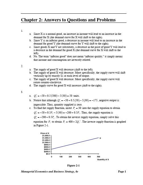
c. At the given prices, quantity demanded is 700 units:
Qxd = 1000 − 2 (154) + .02 (400) = 700 . Substituting the relevant information into
the elasticity formula gives:
EQx ,Px
= −2 Px Qx
= −2 154 700
= −0.44 . Since this is less
Qxd = 1000 − 2 (154) + .02 (400) = 700 . Substituting the relevant information into
the elasticity formula gives:
EQx ,PZ
=
.02
⎛ ⎜ ⎝
PZ Qx
⎞ ⎟ ⎠
=
.02
⎛ ⎜⎝
400 700
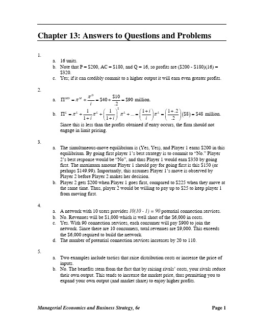
Price $14
$12
$10
$8
$6
$4
$2 Demand
$0
0
1
2
3 MR 4
5
6 Quantity
Figure 3-1
Managerial Economics and Business Strategy, 6e
Page 1
2. a. At the given prices, quantity demanded is 700 units:
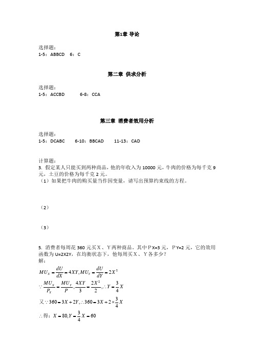
Lower 95% Upper 95%
-880.56 1,254.86
-5.69
-2.96
0.05
0.14
a. Qxd = 187.15 − 4.32Px + .09M .
b. Only the coefficients for the Price of X and Income are statistically significant at the 5 percent level or better.
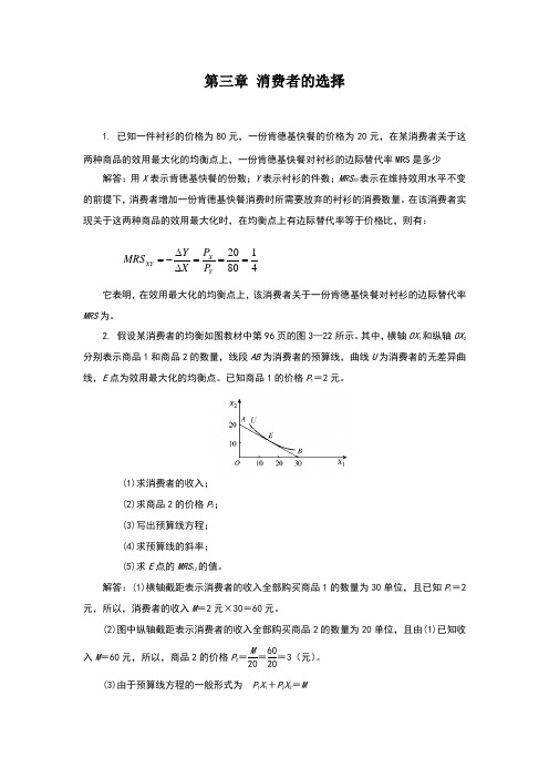
Qxd = 1000 − 2 (354) + .02 (400) = 300 . Substituting the relevant information into
the
elasticity
formula
gives:
EQx ,Px
=
−2
⎛ ⎜ ⎝
Px Qx
⎞ ⎟ ⎠
=
−2
⎛ ⎜⎝
354 300
⎞ ⎟⎠
⎞ ⎟⎠
=
0.011
.
Since
this
number is positive, goods X and Z are substitutes.
3. a. The own price elasticity of demand is simply the coefficient of ln Px, which is – 0.5. Since this number is less than one in absolute value, demand is inelastic. b. The cross-price elasticity of demand is simply the coefficient of ln Py, which is – 2.5. Since this number is negative, goods X and Y are complements. c. The income elasticity of demand is simply the coefficient of ln M, which is 1. Since this number is positive, good X is a normal good. d. The advertising elasticity of demand is simply the coefficient of ln A, which is 2.
Chapter 3: Answers to Questions and Problems
1. a. When P = $12, R = ($12)(1) = $12. When P = $10, R = ($10)(2) = $20. Thus, the price decrease results in an $8 increase in total revenue, so demand is elastic over this range of prices. b. When P = $4, R = ($4)(5) = $20. When P = $2, R = ($2)(6) = $12. Thus, the price decrease results in an $8 decrease total revenue, so demand is inelastic over this range of prices. c. Recall that total revenue is maximized at the point where demand is unitary elastic. We also know that marginal revenue is zero at this point. For a linear demand curve, marginal revenue lies halfway between the demand curve and the vertical axis. In this case, marginal revenue is a line starting at a price of $14 and intersecting the quantity axis at a value of Q = 3.5. Thus, marginal revenue is 0 at 3.5 units, which corresponds to a price of $7 as
Michael R. Baye
d. Use the income elasticity of demand formula to write %ΔQxd = 3 . Solving, we −3
see that the demand of good X will decrease by 9 percent if income decreases by 3 percent.
4. a. Use the own price elasticity of demand formula to write %ΔQxd = −2 . Solving, 5 we see that the quantity demanded of good X will decrease by 10 percent if the price of good X increases by 5 percent. b. Use the cross-price elasticity of demand formula to write %ΔQxd = −6 . Solving, 10 we see that the demand for X will decrease by 60 percent if the price of good Y increases by 10 percent. c. Use the formula for the advertising elasticity of demand to write %ΔQxd = 4 . −2 Solving, we see that the demand for good X will decrease by 8 percent if advertising decreases by 2 percent.
Managerial Economics and Business Strategy, 6e
Page 3
8. The approximate 95 percent confidence interval for a is aˆ ± 2σ aˆ = 10 ± 2 . Thus, you can be 95 percent confident that a is within the range of 8 and 12. The approximate 95 percent confidence interval for b is bˆ ± 2σ bˆ = −2.5 ± 1 . Thus, you can be 95 percent confident that b is within the range of –3.5 and –1.5.
c. The R-square is fairly low, indicating that the model explains only 39 percent of the total variation in demand for X. The adjusted R-square is only marginally lower (37 percent), suggesting that the R-square is not the result of an excessive number of estimated coefficients relative to the sample size. The F-statistic, however, suggests that the overall regression is statistically significant at better than the 5 percent level.