matalb矩阵计算(MATLAB矩阵计算)
MATLAB矩阵及运算

重点
y矩阵中每一列最大的值
y向量中最大的值
最大值的位置
最大值的位置
注意:输入矩阵类型不同, 则执行的操作不同。
2.1.4 函数
因为matlab函数太多,所以要养成使用help
命令,得到有关函数的具体用法:
例:help max
2.1表达式
表达式
(即语句):将变量、数值、函 数用操作符连接起来,就构成了表达式 。
应用:可以和其它语言程序进行数据通信。 举例:
通过MATLAB提供的函数产生矩阵
用内部函数可生成一些特殊矩阵 (函数见书上P50)
重点
通过MATLAB提供的函数产生矩阵
1、单位矩阵(
E方阵)和广义单位矩阵的
产生
重点
通过MATLAB提供的函数产生矩阵
2、随机数矩阵的产生
随机数的产生常常用在控制系统仿真以 及信号分析,是一个非常重要的手段。 MATLAB提供了很好的随机数产生函数: rand() randn()
A/ B A*B
1
A\B A
重点
1
*B
Matlab右除法表示形式:
C=A/B 或 C=A * i n v ( B )
Matlab左除法表示形式: C=A\B 或 C=i n v ( A ) * B
注意:只有行列式不为0的方阵才存在逆阵!!!
矩阵元素的右除、左除
a1 A a3 a2 a4
2)变量名由字母、数字和下划线构成。第一个 字母必须是英文字母。 3)有字符个数限制(版本5.0 :最多31个字符)
2.1.2 变量
MAT
重点
(注意大小写!)
i或j: 错误:5+j7
第三章_matlab矩阵运算

主讲:陈孝敬 E-mail:chenxj9@
第3章
数学运算
主要内容:
①矩阵运算; ②矩阵元素运算;
3.1 矩阵运算
3.1.1 矩阵分析
1.向量范式定义:
x x x
1
n
k 1
xk
2 k
2
k 1 n
x
n
1/ 2
k 1
xk
向量的3种常用范数及其计算函数 在MATLAB中,求向量范数的函数为: (1) norm(V)或norm(V,2):计算向量V的2—范数。 (2) norm(V,1):计算向量V的1—范数。 (3) norm(V,inf):计算向量V的∞—范数。
3.1.2 矩阵分解
矩阵分解:把矩阵分解成比较简单或对它性质比较熟悉的若干 矩阵的乘积的形式;
1.Cholesky分解: Cholesky分解是把对称正定矩阵表示成上三角矩阵的转 置与其本身的乘积,即:A=RTR,在Matlab中用函数chol 来计算Cholesky分解 例3-13 求矩阵A=pascal(4)的Cholesky分解, A=pascal(4) R=chol(A) R’*R
例3-18.求解方程组
x1 x2 3 x3 x4 1 3 x1 x2 3 x3 4 x4 4 x 5x 9 x 8x 0 2 3 4 1
解 先用Matlab函数null求出对应的齐次线性方程组的基础解 系,再利用其系数矩阵的上、下三角阵求出方程组的一个特解, 这样即可得到该方程组的通解,程序如下: >> >> >> >> >> >> A=[1 1 -3 -1;3 -1 -3 4;1 5 -9 -8]; b=[1 4 0] ′; format rat C=null(A , ′r′); %求基础解系 [L,U]=lu(A); %A=LU,L为上三角阵,U为下三角阵 X0= U\(L\b) %用LU求出一个齐次方程的特解
Matlab矩阵运算基础数值运算

data =
1.1000 3.0000 4.0000
2.3000 2.0000 1.0000
.
13
3.2 矩阵运算
主要介绍矩阵的算术运算、关系运算、逻辑 运算和常用的有关矩阵的其他运算(矩阵的 逆,矩阵的秩、矩阵的分解等)。
.
14
3.2.1 矩阵的算术运算
1、矩阵的加(+)减(-)运算:
A±B 矩阵A和矩阵B的和与差,即矩阵相应 位置的元素相加、减。
>> A=magic(3)
D=
A= 816
0.5492 0.2421 -0.6520 0.9075
357
1.0047 -0.4941
492
>> C*D
>> B=inv(A)
ans =
B=
1.0000 0.0000
0.1472 -0.1444 0.0639
0.0000 1.0000
-0.0611 0.0222 0.1056
~ A 对单个矩阵或标量进行取反运算,结果是0-1矩阵。
.
28
3.2.3 矩阵的逻辑运算
例3-11 1 0 3
1 2 0
A2.6 1 2, B0 5 0
0 3 1
1 0 1
计算 A&B, A|B, ~A Nhomakorabea.
29
3.2.4 矩阵函数
1、矩阵的共轭
MATLAB中求矩阵的共轭矩阵的函数是conj,其 调用格式为:
除或浮点溢出都不按错误处理,只是给出警告信息,同时用“Inf”
标记。
.
20
3.2.1 矩阵的算术运算
4、 矩阵的幂运算:^ A^B A的B次方。
matlab矩阵与线性变换与计算

05
实例演示
矩阵的基本操作实例
矩阵的创建
使用方括号[],例如A = [1 2; 3 4]。
矩阵的加法
使用加号+,例如B = [5 6; 7 8],则A + B = [6 8; 10 12]。
矩阵的数乘
使用标量乘法,例如2 * A = [2 4; 6 8]。
矩阵的元素运算
使用点运算符.,例如A.^2 = [1 4; 9 16]。
矩阵计算实例
行列式计算
使用det函数,例如det(A) = -2。
行最简形式
使用rref函数,例如rref(A) = [1 0; 0 1]。
矩阵的逆
使用inv函数,例如inv(A) = [-2 -3; 1.5 0.5]。
矩阵的转置
使用'运算符,例如A' = [1 3; 2 4]。
THANKS
感谢观看
Matlab矩阵与线性变换与计 算
• Matlab矩阵基础 • 线性变换 • 矩阵计算 • Matlab中的矩阵与线性变换操作 • 实例演示
01
Matlab矩阵基础
矩阵的定义与表示
矩阵是一个由数字组 成的矩形阵列,行和 列的数量可以不同。
还可以使用分号来分 隔行,以创建多行矩 阵。
在Matlab中,可以 使用方括号[]来创建 矩阵,并使用逗号分 隔行内的元素。
矩阵的基本操作
加法
将两个矩阵的对应元素相加。
减法
将一个矩阵的对应元素减去另 一个矩阵的对应元素。
数乘
将一个标量与矩阵中的每个元 素相乘。
转置
将矩阵的行和列互换。
特殊类型的矩阵
对角矩阵
除了主对角线上的元素外,其他元素都为零 的矩阵。
第2章 matlab矩阵及其运算

第2章 MATLAB 矩阵及其运算
2.1.2 MATLAB常用数学函数
MATLAB提供了许多数学函数,函
数的自变量规定为矩阵变量,运算法
则是将函数逐项作用于矩阵的元素上, 因而运算的结果是一个与自变量同维
数的矩阵。
11/128 MALAB 7.X程序设计
第2章 MATLAB 矩阵及其运算
1. 三角函数 • sin 正弦函数 • asin 反正弦函数 • cos 余弦函数 • tan 正切函数 • cot 余切函数 • sec 正割函数 • csc 余割函数
在MATLAB命令口输入命令:
x=1+2i; y=3-sqrt(17); z=(cos(abs(x+y))-sin(78*pi/180))/(x+abs(y))
其中pi和i都是MATLAB预先定义的变量,分别
代表代表圆周率π和虚数单位。 输出结果是:
z =
-0.3488 + 0.3286i
10/128 MALAB 7.X程序设计
18/128 MALAB 7.X程序设计
第2章 MATLAB 矩阵及其运算
rem与mod的区别
rem(x,y)=x-y.*fix(x./y)
mod(x,y)=x-y.*floor(x./y)
eg: >>x=5;y=3; >>y1=rem(x,y),y2=mod(x,y) >> x=-5;y=3; >>y1=rem(x,y),y2=mod(x,y)
%绝对值 %取复数虚部 %取复数实部 %复数共轭
16/128 MALAB 7.X程序设计
第2章 MATLAB 矩阵及其运算
4. 取整函数 fix(x) 朝零方向取整 floor(x) 朝负无穷大方向取整 ceil(x) 朝正无穷大方向取整 round(x)四舍五入 mod(x,y) rem(x,y)取x/y的余数要求x,y 必须为相同大小的实矩阵或为标量。 eg: x=5.3 x=-5.3 -5.3 -5 0 5 5.3
matlab矩阵乘法
matlab矩阵乘法MATLAB(MatrixLaboratory)是一款常用的科学运算计算软件包,用它开发的应用程序可以用于数学、统计、优化、仿真等领域。
MATLAB 中的矩阵乘法是MATLAB的基本计算操作,是能够实现向量和矩阵的运算。
一、矩阵乘法的定义矩阵乘法是指两个同样大小的矩阵相乘,按照一定的计算公式,得到一个新的矩阵。
因为大多数数学问题都可以用矩阵表示,所以用矩阵乘法可以把复杂的运算简化成一步计算,这在大量数字计算中很有帮助。
矩阵乘法的计算公式如下:设A是m×n矩阵,B是n×p矩阵,则A×B=C是m×p矩阵,其中:$$C_{ij} = sum_{k=1}^{n}A_{ik}B_{kj}$$二、MATLAB的矩阵乘法MATLAB中的矩阵乘法主要提供了三种矩阵乘法指令,即“*”、“.*”、“times”。
1、*”和“.*”“*”是矩阵标准乘法运算符,是指矩阵相乘时,最常用的形式,其计算公式如上所述,但要求两个矩阵的列数一致。
而“.*”则是矩阵的点乘法,即每个元素分别相乘,而不是矩阵乘法,其计算公式为:$$C_{ij} = A_{ij} times B_{ij}$$2、“times”“times”是MATLAB中的特殊形式矩阵乘法。
它接受两个参数,一个是要求被乘数A是m×n矩阵,另一个要求乘数B是n×1向量,计算公式如下:$$C_{ij} = sum_{k=1}^{n}A_{ik}B_{k}$$三、MATLAB中矩阵乘法的应用在各类应用软件中,MATLAB的矩阵乘法有着广泛的应用,主要应用于数据处理、优化计算以及机器学习等领域。
1、数据处理采用矩阵乘法可以实现数据的简单处理,例如矩阵的转置与行列重排。
2、优化问题矩阵乘法可以用于求解复杂优化问题,比如最小二乘法拟合问题、最小角回归问题等,这些优化问题也可以通过矩阵乘法的形式进行解算,大大提高了运算的效率。
Matlab 矩阵的运算
(1) 矩阵加减运算 假定有两个矩阵A和B,则可以由A+B和 A-B实现矩阵的加减运算。 运算规则是:若A和B矩阵的维数相同, 则可以执行矩阵的加减运算,A和B矩阵的相 应元素相加减。如果A与B的维数不相同,则 MATLAB将给出错误信息,提示用户两个矩 阵的维数不匹配。 (2) 矩阵乘法 假定有两个矩阵A和B,若A为m×n矩阵, B为n×p矩阵,则C=A*B为m×p矩阵。
关系运算符的运算法则为: (1) 当两个比较量是标量时,直接比较两 数的大小。若关系成立,关系表达式结果为1, 否则为0。 (2) 当参与比较的量是两个维数相同的矩 阵时,比较是对两矩阵相同位置的元素按标 量关系运算规则逐个进行,并给出元素比较 结果。最终的关系运算的结果是一个维数与 原矩阵相同的矩阵,它的元素由0或1组成。
例3-3 先建立 5×5矩阵A,然后将A的第一 行元素乘以1,第二行乘以2,…,第五行乘 以5。 A=[17,0,1,0,15;23,5,7,14,16;4,0,13,0,22; 10,12,19,21,3;11,18,25,2,19]; D=diag(1:5); D*A %用D左乘A,对A的每行 乘以一个指定常数
3.3 字符串
在MATLAB中,字符串是用单撇号(‘)括 起来的字符序列。 MATLAB 将字符串当作一个行向量, 每个元素对应一个字符,其标识方法和数值 向量相同。也可以建立多行字符串矩阵。
字符串是以ASCII码形式存储的。abs和 double函数都可以用来获取字符串矩阵所对 应的ASCII码数值矩阵。 相反,char函数可以把ASCII码矩阵转换 为字符串矩阵。
3.2.4 方阵的行列式
把一个方阵看作一个行列式,并对其按 行列式的规则求值,这个值就称为矩阵所对 应的行列式的值。 在MATLAB中,求方阵A所对应的行列 式的值的函数是det(A)。
matlab矩阵乘法

matlab矩阵乘法众所周知,矩阵是数学、计算机科学等专业的基础知识之一。
但是由于我们学习矩阵的时间太短,导致很多同学都觉得矩阵比较难理解。
其实,矩阵不仅有它自己独特的魅力,更重要的是能帮助我们理解矩阵的性质。
在众多科学领域中,矩阵是使用最广泛的数据结构。
所以,我们应该利用好矩阵,让矩阵发挥它最大的价值。
那么, matlab有什么好的矩阵功能来辅助我们学习矩阵呢?下面,我们就来简单了解一下。
MATLAB矩阵乘法可分为两类:矩阵运算和矩阵变换。
矩阵运算通过运算符(+,-,*,/)完成,用以实现矩阵之间的加减乘除运算。
对于矩阵A,先按照A行变换到B列,再执行A列变换到B行。
矩阵变换则通过矩阵的某些特征进行矩阵之间的相乘或转置操作。
这种方法适合于一般矩阵的变换。
矩阵乘法通过矩阵的所有元素与矩阵相乘得到矩阵的乘积,然后将乘积输出到屏幕上。
MATLAB还提供了矩阵的幂、方根、倒数、迹等功能。
这些功能均可通过矩阵乘法完成。
矩阵运算与矩阵变换的区别如下:matlab的矩阵数组类似于数组,但数组只能一次性存储1维或2维的数据。
矩阵数组可以包含多维数据,即矩阵数组中的元素是由若干个矩阵元素组成的。
例如,假设有三个二维矩阵元素A, B和C,那么矩阵数组3维数组( A, B, C)中的第三个元素D就是由矩阵元素C和C组成。
matlab也提供了矩阵数组转矩阵数组的功能,例如矩阵数组A转矩阵数组B。
当用matlab进行矩阵运算或矩阵变换时,我们可以使用矩阵的运算符(+,-,*, /)进行运算或者矩阵的某些特征(如倒数,迹)进行矩阵之间的相乘或转置操作。
例如:matlab的矩阵乘法是对矩阵进行矩阵的运算,比如求两个矩阵的积,而矩阵变换则是对矩阵进行矩阵的变换,即矩阵的乘法。
而且矩阵运算中还包括求矩阵的逆矩阵。
对于一般矩阵来说,矩阵的运算或矩阵的变换效率高,但是对于复杂矩阵而言,运算或变换的速度就相对较慢,因此矩阵乘法是不适用于计算一般矩阵的,通常只用来对矩阵进行快速运算。
第2章 MATLAB矩阵及其运算

floor:下取整 ceil:上取整 round:四舍五入取整
(4) rem与mod函数的区别:
rem(x,y): 求余数 mod(x,y):模除求余 x,y必须为相同大小的实矩阵或为标量
x=abs(-4.56), y=abs(3+4i), z=abs('a') x=2.45; y1=fix(x),y2=floor(x),y3=ceil(x),y4=round(x) x=-2.65; y1=fix(x),y2=floor(x),y3=ceil(x),y4=round(x) x=5;y=3; y1=rem(x,y),y2=mod(x,y) x=-5;y=3; y1=rem(x,y),y2=mod(x,y)
(2) 矩阵乘法 假定有两个矩阵A和B,若A为m×n矩阵, B为n×p矩阵,则C=A*B为m×p矩阵。
(3) 矩阵除法 在MATLAB中,有两种矩阵除法运算:\和/,分别表 示左除和右除。 如果A矩阵是非奇异方阵,则A\B和B/A运算可以实现。 A\B等效于A的逆左乘B矩阵,也就是inv(A)*B, B/A等效于A矩阵的逆右乘B矩阵,也就是B*inv(A) 对于含有标量的运算,两种除法运算的结果相同,如 3/4和4\3有相同的值,都等于0.75。 a=[10.5,25],则a/5=5\a=[2.1000 5.0000]。 对于矩阵运算,一般A\B≠B/A。
2.1.5 数据的输出格式
Matlab用十进制数表示一个常数
采用日常记数法、科学记数法
3.1415, -9.5i, 3+5i; 1.78029e2, 6.732E2i, 1234e-3-5i %e, E 表以10为底的指数
MATLAB内部每一个数据元素都是用双精度数来 表示和存储的 可以用format命令设置或改变数据输出格式。 format命令的格式为: format 格式符 其中格式符决定数据的输出格式
matlab求解矩阵方程算法

matlab求解矩阵方程算法
求解矩阵方程是线性代数中的一个重要问题,在Matlab中有多种方法可以用来求解矩阵方程。
其中最常用的方法包括直接法和迭代法。
1. 直接法:
a. 逆矩阵法,如果方程为AX=B,其中A是一个可逆矩阵,那么可以通过求解X=A^(-1)B来得到解。
在Matlab中可以使用inv 函数求逆矩阵,然后进行矩阵乘法得到解。
b. 左除法,Matlab中可以使用左除法运算符“\”来求解矩阵方程,即X=A\B。
2. 迭代法:
a. Jacobi迭代法,Jacobi迭代法是一种基本的迭代法,通过不断迭代更新矩阵X的值,直到满足一定的精度要求为止。
在Matlab中可以编写循环来实现Jacobi迭代法。
b. Gauss-Seidel迭代法,类似于Jacobi迭代法,但是每次更新后立即使用最新的值进行计算,可以加快收敛速度。
c. 共轭梯度法,对于对称正定矩阵方程,可以使用共轭梯度法进行求解。
Matlab中提供了conjugateGradient函数来实现共轭梯度法求解矩阵方程。
除了上述方法外,Matlab还提供了一些特定类型矩阵方程的求解函数,比如求解特征值和特征向量的eig函数,求解奇异值分解的svd函数等。
总之,根据具体的矩阵方程类型和求解精度要求,可以选择合适的方法在Matlab中求解矩阵方程。
希望这些信息能够帮助到你。
Matlab 矩阵运算
Matlab 矩阵运算说明:这一段时间用Matlab做了LDPC码的性能仿真,过程中涉及了大量的矩阵运算,本文记录了Matlab中矩阵的相关知识,特别的说明了稀疏矩阵和有限域中的矩阵。
Matlab的运算是在矩阵意义下进行的,这里所提到的是狭义上的矩阵,即通常意义上的矩阵。
目录第一部分:矩阵基本知识一、矩阵的创建1.直接输入法2.利用Matlab函数创建矩阵3.利用文件创建矩阵二、矩阵的拆分1.矩阵元素2.矩阵拆分3.特殊矩阵三、矩阵的运算1.算术运算2.关系运算3.逻辑运算四、矩阵分析1.对角阵2.三角阵3.矩阵的转置与旋转4.矩阵的翻转5.矩阵的逆与伪逆6.方阵的行列式7.矩阵的秩与迹8.向量和矩阵的范数9.矩阵的特征值与特征向量五、字符串六、其他第二部分矩阵的应用一、稀疏矩阵1.稀疏矩阵的创建2.稀疏矩阵的运算3.其他二、有限域中的矩阵内容第一部分:矩阵基本知识(只作基本介绍,详细说明请参考Matlab帮助文档)矩阵是进行数据处理和运算的基本元素。
在MATLAB中a、通常意义上的数量(标量)可看成是”1*1″的矩阵;b、n维矢量可看成是”n*1″的矩阵;c、多项式可由它的系数矩阵完全确定。
一、矩阵的创建在MATLAB中创建矩阵有以下规则:a、矩阵元素必须在”[ ]“内;b、矩阵的同行元素之间用空格(或”,”)隔开;c、矩阵的行与行之间用”;”(或回车符)隔开;d、矩阵的元素可以是数值、变量、表达式或函数;e、矩阵的尺寸不必预先定义。
下面介绍四种矩阵的创建方法:1、直接输入法最简单的建立矩阵的方法是从键盘直接输入矩阵的元素,输入的方法按照上面的规则。
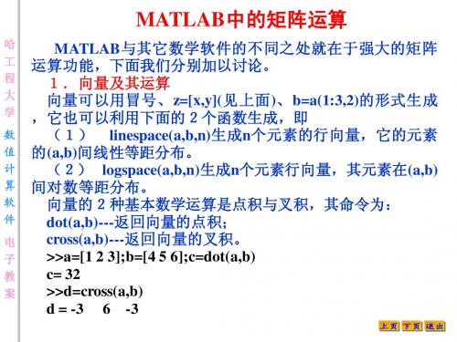
建立向量的时候可以利用冒号表达式,冒号表达式可以产生一个行向量,一般格式是: e1:e2:e3,其中e1为初始值,e2为步长,e3为终止值。
还可以用linspace函数产生行向量,其调用格式为:linspace(a,b,n) ,其中a和b 是生成向量的第一个和最后一个元素,n是元素总数。
MATLAB矩阵

4.内存变量的管理
2)clear命令------用于删除MATLAB工作空间中的 变量。 3)who和whos命令------用于显示在MATLAB工作 空间中已经驻留的变量名清单。 who命令只显示出驻留变量的名称 whos在给出变量名的同时,还给出它们的大 小、所占字节数及数据类型等信息。 4)CLC————可以清屏
2.矩阵的修改
1)直接修改:可用键找到所要修改的矩阵, 用键移动到要修改的矩阵元素上即可修 改。 2)指令修改:可以用A(,)= 来修改。
2 1022
二、创建矩阵
5.采用定数对数采样函数产生向量 其调用格式为: y=logspace(a,b,n);其中a和b是 生成向量的第一个和最后一个元素,n是元素总数。 其作用是10^a和10^b之间产生一等分的n维向量, 如果省略n,则系统默认n等于50. 如x=logspace(0,5,6);x=logspace(0,5)
Hale Waihona Puke 4.内存变量的管理1) 内存变量的删除与修改 MATLAB工作空间窗口专门用于内存变量的 管理。在工作空间窗口中可以显示所有内存变 量的属性。当选中某些变量后,再单击Delete 按钮,就能删除这些变量。当选中某些变量后, 再单击Open按钮,将进入变量编辑器。通过变 量编辑器可以直接观察变量中的具体元素,也 可修改变量中的具体元素。
1.矩阵和数组拆分
A(:,j)表示取A矩阵的第j列全部元素; A(i,:)表示A矩阵第i行的全部元素; A(i:i+m,:)表示取A矩阵第i~i+m行的全
部元素; A(:,k:k+m)表示取A矩阵第k~k+m列 的全部元素;
1.矩阵和数组拆分
A(i:i+m,k:k+m)表示取A矩阵第i~i+m行内,并在第
MATLAB中的矩阵运算
哈 工 程 大 学 数 值 计 算 软 件
●randn生成正态分布的随机阵 生成正态分布的随机阵 randn(n)生成 ×n的正态随机阵; 生成n× 的正态随机阵 的正态随机阵; 生成 randn(m,n),randn([m,n])生成 ×n的正态随机阵; 生成m× 的正态随机阵 的正态随机阵; 生成 randn(size(A))生成与矩阵 大小相同的正态随机阵。 生成与矩阵A大小相同的正态随机阵 生成与矩阵 大小相同的正态随机阵。 (5)其它基本运算 左右翻转; 上下翻转; ●fliplr(A) 将A左右翻转;●flipud(A) 将A上下翻转; 左右翻转 上下翻转 旋转90度 返回A ● rot90(A) 将 A旋转 度 。 ● tril(A)返回 A 的下三角部分 ; 旋转 返回 的下三角部分; tril(A,k)返回A第K 条对角线以下部分,K=0为主对角线, 返回A 条对角线以下部分,K=0为主对角线, 返回 K>0为主对角线以上,K<0为主对角线以下。 K>0为主对角线以上,K<0为主对角线以下。 返回A ●triu(A), triu(A,K)返回A的上三角部分,其它同上。 返回 的上三角部分,其它同上。 返回以向量v为主对角线的矩阵 ●diag(v)返回以向量 为主对角线的矩阵; 返回以向量 为主对角线的矩阵; diag(v,k) 若 v 是 n 个 元 素 的 向 量 , 则 它 返 回 一 个 大 小 为 n+abs(k)方阵,向量 位于第 条对角线上。K=0代表主对角线 方阵, 位于第k条对角线上 方阵 向量v位于第 条对角线上。 代表主对角线 为主对角线以上, 为主对角线以下。 , k>0为主对角线以上,k<0为主对角线以下。 diag(A)以向量 为主对角线以上 为主对角线以下 以向量 形式, 返回A 的主对角线元素; 对于矩阵A 形式 , 返回 A 的主对角线元素 ; diag(A,k)对于矩阵 A , 返回 对于矩阵 由第k条对角线构成的列向量 条对角线构成的列向量。 由第 条对角线构成的列向量。
MATLAB的矩阵运算

MATLAB的矩阵运算阅读⽬录 MATLAB是基于矩阵和数组计算的,可以直接对矩阵和数组进⾏整体的操作,MATLAB有三种矩阵运算类型:矩阵的代数运算、矩阵的关系运算和矩阵的逻辑运算。
其中,矩阵的代数运算应⽤最⼴泛。
本⽂主要讲述矩阵的基本操作,涉及矩阵的创建、矩阵的代数运算、关系运算和逻辑运算等基本知识。
矩阵的创建直接输⼊法创建矩阵% 1. 直接输⼊法创建矩阵>> A = [1,2,3; 4,5,6; 7,8,9]A =1 2 34 5 67 8 9函数法创建矩阵简单矩阵% 2. 函数法创建矩阵>> zeros(3)% ⽣成3x3的全零矩阵ans =0 0 00 0 00 0 0>> zeros(3,2)% ⽣成3x2的全零矩阵ans =0 00 00 0>> eye(3)% ⽣成单位矩阵ans =1 0 00 1 00 0 1>> ones(3)% ⽣成全1矩阵ans =1 1 11 1 11 1 1>> magic(3)% ⽣成3x3的魔⽅阵ans =8 1 63 5 74 9 2>> diag(1:3)% 对⾓矩阵ans =1 0 00 2 00 0 3>> diag(1:5,1)% 对⾓线向上移1位矩阵ans =0 1 0 0 0 0 0 0 2 0 0 0 0 0 0 3 0 0 0 0 0 0 4 0 0 0 0 0 0 5 0 0 0 0 0 0 >> diag(1:5,-1)% 对⾓线向下移1位矩阵ans =0 0 0 0 0 01 0 0 0 0 0 02 0 0 0 0 0 03 0 0 0 0 0 04 0 0 0 0 0 05 0 >> triu(ones(3,3))% 上三⾓矩阵ans =1 1 10 1 10 0 1>> tril(ones(3,3))% 下三⾓矩阵ans =1 0 01 1 01 1 1随机矩阵>> rand(3)% ⽣成随机矩阵ans =0.2898 0.8637 0.05620.4357 0.8921 0.14580.3234 0.0167 0.7216>> rand('state',0); % 设定种⼦数,产⽣特定种⼦数下相同的随机数>> rand(3)ans =0.9501 0.4860 0.45650.2311 0.8913 0.01850.6068 0.7621 0.8214>> a = 1; b = 100;>> x = a + (b-a)* rand(3)% 产⽣区间(1,100)内的随机数x =38.2127 20.7575 91.113389.9610 31.0064 53.004043.4711 54.2917 31.3762>> a = 1; b = 100;>> a + fix(b * rand(1,50))% 产⽣50个[1,100]内的随机正整数ans =列 1 ⾄ 154 72 77 6 63 27 32 53 41 90 58 57 40 70 57列 16 ⾄ 3035 60 28 5 84 11 73 45 100 57 47 42 22 24 32列 31 ⾄ 4587 26 97 31 38 35 71 62 76 80 22 90 90 94 28列 46 ⾄ 5048 26 37 53 39相似函数扩展>> randn(3)% ⽣成均值为0,⽅差为1的正太分布随机数矩阵ans =-0.4326 0.2877 1.1892-1.6656 -1.1465 -0.03760.1253 1.1909 0.3273>> randperm(10)% ⽣成1-10之间随机分布10个正整数ans =4 9 10 25 8 1 3 7 6% 多项式x^3 - 7x + 6 的伴随矩阵>> u = [1,0,-7,6];>> A = compan(u)% ⽣成伴随矩阵A =0 7 -61 0 00 1 0>> eig(A) % 此处eig()函数⽤于求特征值% 利⽤伴随矩阵求得⽅程的根ans =-3.00002.00001.0000矩阵的运算矩阵的代数运算矩阵的算术运算>> A = [1,1;2,2];>> B = [1,1;2,2];>> AA =1 12 2>> BB =1 12 2>> A + Bans =2 24 4>> B-Aans =0 00 0>> A * Bans =3 36 6>> A^2ans =3 36 6>> A^3ans =9 918 18矩阵的运算函数>> C = magic(3)C =8 1 63 5 74 9 2>> size(C)ans =3 3>> length(C)ans =3>> sum(C)ans =15 15 15>> max(C)ans =8 9 7>> C'ans =8 3 41 5 96 7 2>> inv(C)ans =0.1472 -0.1444 0.0639 -0.0611 0.0222 0.1056 -0.0194 0.1889 -0.1028矩阵的元素群运算元素群运算,是指矩阵中的所有元素按单个元素进⾏运算,也即是对应位置进⾏运算。
第2章 MATLAB矩阵及其运算
1 4 7 1 4 7
3 5 6 8 9 11 2 3 5 6 8 9
2.2.2 矩阵的拆分
1.矩阵元素的引用方式
1)通过下标引用矩阵的元素,例如
A=[1,2,3;4,5,6;7,8,9] A(3,2)=200 注意 :如果给出的下标大于矩阵的行数和列数,则 自动扩展原有矩阵,没赋值的元素为0。
元素由1,2,3,…,n2共n2个整数组成。MATLAB提供
了求魔方矩阵的函数magic(n),其功能是生成一个 n阶魔方阵。 (2) 范得蒙矩阵 (3) 希尔伯特矩阵 (4) 托普利兹矩阵 (5) 伴随矩阵
(6) 帕斯卡矩阵
练习
1.利用clear命令清除工作空间的变量(若工作 空间没有变量,可先任意新建一个); 2.按下列方式对变量赋值 A=[pi,2*pi;4*pi,0;10*pi,0.5*pi]; B=[1+2i,3-5i,5;4,6-2i,8;7,9+3i,11]; 3.求出2题中A的正弦函数并赋给变量C,求出 2题中B的实部和虚部分别赋给变量Br和Bi。 4.将3题中的变量C, Br和Bi保存下来,保存 数据的文件名自己选取(英文名)
1.变量命名
可以改变, 重新赋值
在MATLAB 中,变量名是以字母开头,后接字母、
数字或下划线的字符序列(不能包含空格和标点
符号),最多63个字符。在MATLAB中,变量名 区分字母的大小写。关键字和函数名不能作为变 量名。
2.赋值语句 (1) 变量=表达式 (2) 表达式
其中表达式是用运算符将有关运算量连接起来的
e或E表示 10为底的 指数
e3,2e3, 1e, 1e-2, 1E2, 1E-2i, 2E-1-i, .....
matlab计算协方差矩阵
matlab计算协方差矩阵协方差矩阵是一种用于衡量两个或多个变量之间关系的统计工具。
在Matlab中,可以使用cov函数来计算协方差矩阵。
cov函数的语法如下:C = cov(X)其中,X是一个n×p维的矩阵,每一列代表一个变量,每一行代表一次测量。
C是一个p×p的协方差矩阵,其中C(i,j)表示变量i和变量j之间的协方差。
下面我们将详细介绍如何使用Matlab计算协方差矩阵:步骤1:创建一个输入矩阵X。
假设我们有三个变量X1、X2和X3,每个变量有五次测量。
可以使用以下代码创建输入矩阵:```X=[1,2,3;4,5,6;7,8,9;10,11,12;13,14,15];```这将创建一个5×3的矩阵,其中每一列代表一个变量,每一行代表一次测量。
步骤2:使用cov函数计算协方差矩阵。
可以使用以下代码计算协方差矩阵:```C = cov(X);```这将返回一个3×3的矩阵C,其中C(i,j)表示变量i和变量j之间的协方差。
步骤3:打印协方差矩阵。
可以使用以下代码打印协方差矩阵:```disp(C);```这将打印出协方差矩阵的值。
完整的代码示例如下:```X=[1,2,3;4,5,6;7,8,9;10,11,12;13,14,15];C = cov(X);disp(C);```以上代码将计算三个变量之间的协方差矩阵,并将其打印出来。
在实际应用中,协方差矩阵可以用于许多目的,例如探索变量之间的相关性、计算主成分分析等。
通过计算协方差矩阵,我们可以获得有关数据集的更多信息,以便进行进一步的分析和处理。
实验1 MATLAB矩阵计算
显示结果:
V =
0.7130 0.2803 0.2733
-0.6084 -0.7867 0.8725
0.3487 0.5501 0.4050
D =
-25.3169 0 0
0 -10.5182 0
0 0 16.8351
B=
1 0 0 3 3
0 1 0 3 3
0 0 1 3 3
0 0 0 2 2
0 0 0 2 2
6.建立一个5 5的矩阵,求它的行列式值、迹、秩和范数
命令:>>A=fix(10*rand(5))
B=det(A)
C=trace(A)
D=rank(A)
E=norm(A)
显示结果:B=
0
C=
5
D=
5
E=
5
7.已知 ,求A的特征值及特征向量。
显示结果:
(1)x =
1.2000
0.6000
0.6000
(2)新解为:
x =
3.0000
-6.6000
6.6000
比较解的相对变化情况:x1,x2, x3均变化
(3)条件数为:
C1 =
2.0150e+003
C2 =
1.3533e+003
C3 =
2.0150e+003
分析结论:
9.建立矩阵A,试比较sqrtm(A)和sqrt(A),分析它们的区别
命令:A+6*B
显示结果:18 52 -10
46 7 105
21 53 49
(2)A*B和A.*B
Matlab 教程第2章 MATLAB矩阵及其运算
H=invhilb(4)
(4) 托普利兹矩阵 托普利兹(Toeplitz)矩阵除第一行第一列外, 其他每个元素都与左上角的元素相同。生 成托普利兹矩阵的函数是toeplitz(x,y),它 生成一个以x为第一列,y为第一行的托普 利兹矩阵。这里x, y均为向量,两者不必等 长。toeplitz(x)用向量x生成一个对称的托普 利兹矩阵。例如
它专门建立一个M文件。下面通过一个简 单例子来说明如何利用M文件创建矩阵。
例2-2 利用M文件建立MYMAT矩阵。 (1) 启动有关编辑程序或MATLAB文本编辑 器,并输入待建矩阵:
(2) 把输入的内容以纯文本方式存盘(设文 件名为mymatrix.m)。 (3) 在MATLAB命令窗口中输入mymatrix, 即运行该M文件,就会自动建立一个名为 MYMAT的矩阵,可供以后使用。
M=100+magic(5)
(2) 范得蒙矩阵 范得蒙(Vandermonde)矩阵最后一列全为1, 倒数第二列为一个指定的向量,其他各列 是其后列与倒数第二列的点乘积。可以用 一个指定向量生成一个范得蒙矩阵。在 MATLAB中,函数vander(V)生成以向量V 为基础向量的范得蒙矩阵。例如, A=vander([1;2;3;5])即可得到上述范得蒙矩 阵。
(2) 利用空矩阵删除矩阵的元素 在MATLAB中,定义[]为空矩阵。给变
量X赋空矩阵的语句为X=[]。注意,X=[]与 clear X不同,clear是将X从工作空间中删
除,而空矩阵则存在于工作空间中,只是 维数为0。
2.2.3 特殊矩阵 1.通用的特殊矩阵 常用的产生通用特殊矩阵的函数有:
zeros:产生全0矩阵(零矩阵)。 ones:产生全1矩阵(幺矩阵)。 eye:产生单位矩阵。 rand:产生0~1间均匀分布的随机矩阵。 randn:产生均值为0,方差为1的标准正态 分布随机矩阵。
- 1、下载文档前请自行甄别文档内容的完整性,平台不提供额外的编辑、内容补充、找答案等附加服务。
- 2、"仅部分预览"的文档,不可在线预览部分如存在完整性等问题,可反馈申请退款(可完整预览的文档不适用该条件!)。
- 3、如文档侵犯您的权益,请联系客服反馈,我们会尽快为您处理(人工客服工作时间:9:00-18:30)。
matalb矩阵计算(MATLAB矩阵计算)matalb矩阵计算(MATLAB矩阵计算)4.1 array operations and matrix operationsFrom the appearance of the shape and structure of the data matrix, two-dimensional array and no difference in mathematics. However, as the embodiment of a matrix transformation or mapping operator matrix with mathematical rules, clear and strict. And array operation is defined by the software of MATLAB rules, its purpose is for data management, simple operation. The instruction form nature and perform calculations effectively. Therefore, when using MATLAB, in particular to a clear distinction between clear array operations and matrix operations. Table 4.1.1 lists the similarities and differences between the essence and connotation of two kinds of operation instruction.4.1.1 array operations and matrix operations, instruction forms and substantive meaningArray operationMatrix operationinstructionsMeaninginstructionsMeaningA.'Non conjugate transposeA'Conjugate transposeA=sAssign scalar s to each element of the array AS+BAdd scalar s to each element of the array B, respectivelyS-B, B-sThe difference between the scalar s and the elements of the array B S.*AScalar s is the product of the elements of the array A, respectively S*AThe product of the scalar s and the elements of the matrix A, respectivelyS./B, B.\sScalar s is separated by the elements of array B, respectivelyS*inv (B)Inverse multiplicative scalar B of matrix sA.^nThe N sub order of each element of the array AA^nWhen A is a square matrix, the n power of the matrix AA+BThe addition of an array corresponding elementA+Bmatrix additionA-BSubtracting elements of an arrayA-BMatrix subtractionA.*BMultiplication of an array corresponding elementA*BThe product of the same matrix NevilleA./BThe elements of A are excluded by the corresponding elements of B A/BA right, except BB.\AIt must be the sameB\AA left exceptB (usually different from right division)Exp (A)For the end to e respectively with A elements as index, exponentiationExpm (A)Matrix exponential function of ALog (A)The logarithm of the elements of ALogm (A)The matrix logarithmic function of ASqrt (A)The square root of the elements of the product of ASqrtm (A)A's square function of matricesFrom the above we can see that the array operations such as multiplication, addition, multiplication, transpose, add "points". Therefore, we should pay special attention to "multiply, divide, involution, trigonometric and exponential function", two operations are fundamentally different. In addition, in the implementation of the array and array operation when the array must be involved in computing Tongwei, the result is always with the original array array dimensions.4.2 basic operations of an arrayIn MATLAB, an array operation is a.MATLAB that uses the same calculation for multiple numbers to process arrays in a very intuitive way4.2.1 point transpose and conjugate transpose` - dot transpose. Non conjugate transpose, equivalent to conj (A') A=1:5;'b=a.'= bOneTwoThreeFourFive'c=b.'= C12345This shows that the two transpose of the row vector yields the original row vectorConjugate transpose. Transpose the vectors and conjugate each element:D=a+i*a= DColumns 1 through 31 + 1.0000i2 + 2.0000i3 + 3.0000iColumns 4 through 54 + 4.0000i5 + 5.0000iE=d'= e1 - 1.0000i2 - 2.0000i3 - 3.0000i4 - 4.0000i5 - 5.0000i4.2.2 scalar (scalar) and four operations of an arraySimple mathematical operations can be performed between scalar and array, such as addition, subtraction, multiplication, division, and mixing operations"G=[1 234"567891011 12]G=g-2= g-1 0123456789102*g-1= ans-3 -1 135791113151719Four operations between 4.2.3 arraysIn MATLAB, the array between the four operations, an array of participating in operation must have the same dimension, subtraction, multiplication, addition, operation is carried out according to the elements and elements forms. Among them, the array between the addition, subtraction and matrix addition, subtraction to the same operator, as: "+" "-". However, the array multiplication, division and matrix multiplication, division operation symbol is completely different, thereare differences, between the array multiplication and division operators: "*", "/" or ".".1. array by element add, minus"G=[1 234"567891011 12]"H=[1 111; 2222; 333; 3]"> g+h% added by element= ans23457891012131415> ans-h%, subtract by element= ans123456789 10 11 12> > > > > > > 2 g / h) 混合运算years.1 3 5 78 10 12 1415 17 19 212. 按元素乘> > > > > > > g * hyears.1 2 3 410 12 14 1627 30 33 363. 按元素除数组间的除法运算符有两个, 即左除 "/" 和右除 "." 它们之间的关系是.a /b = b.> > > > > > > g / hyears.1.00002.00003.00004.00002.50003.00004.1000 4.00003.0000 3.3333 3.66674.0000"h \ gyears.1.00002.00003.00004.00002.50003.00004.1000 4.00003.0000 3.3333 3.66674.0000幂运算.在matlab中, 数组的幂运算的运算为 "." 表示每一个元素进行幂运算. > > > > > > > (2% 数组g每个元素的平方.years.1 4 9 425, 36, 49, 6481% (144> > > > > > > g ^ (- 1)) 数组g的每个元素的倒数years.1.0000 0.5000 0.3333 0.25000.2000 0.1667 0.1429 0.12500.1111 0.1000 0.0909 0.0833> > > > > > > 2 g%, 以g的每个元素为指数对2进行乘方运算.years.2 4 8 1632, 64, 128, 256512 1024, 2048, 4096> > > > > > > "h% 以h的每个元素为指数对g中相应元素进行乘方运算.years.1 2 3 425, 36, 49, 64729 1000, 1728> > > > > > > (h - 1).years.1 1 1 1 1 1 1 1 1 1 1 1 1 1 1 1 1 1 1 1 1 15 6 7 881% (144- 数组的指数, 对数和开方运算在matlab中, 所谓数组的运算实质是是数组内部每个元素的运算, 因此, 数组的指数, 对数和开方运算与标量的运算规则完全是一样的, 运算符函数分别为: exp () log (), () must 等.> > a = [1, 3, 4, 5, 2, 6, 3, 2, 4].> > > > > > > c = exp (a)c =2.7183 20.0855 54.59827.3891 403.4288 148.413220.0855 7.3891 54.5982> > > > > > > > > > > >数组的对数, 开方运算与数组的指数运算, 其方式完全一样, 这里不详述.向量运算.对于一行或一列的矩阵, 为向量, matlab有专门的函数来进行向量点积, 叉积和混合积的运算.the 向量的点积运算在高等数学中, 我们知道, 两向量的点积指两个向量在其中一个向量方向上的投影的乘积, 通常用来定义向量的长度.在matlab中, 向量的点积用函数 "dot"来实现, 其调用格式如下.c = dot (a, b) - 返回向量a与b的点积, 结果存放于c中.c = dot (a, b, d) - 返回向量a与b在维数为dim的点积, 结果存放于c中.> > a = [4 2 5 3 1).> > b = (3 8 10 12 13].> > > > > > > c = (a, b).c =137> > > > > > > c = dot (a, b, (4)c =32 50 36 13 6a 向量的叉积运算在高等数学中, 我们知道, 两向量的叉积返回的是与两个向量组成的平面垂直的向量.在matlab中, 向量的点积用函数 cross 来实现, 其调用格式如下.c = cross (a, b) - 返回向量a与b的叉积, 即, 结果存放于c中.c = cross (a, b, d) - 返回向量a与b在维数为dim的叉积, 结果存放于c 中.> > a = [2, 5].> > b = [3, 10].> > > > > > > c = cross (a, b)c =0 - 5 4these 向量的混合运算> > > > > > > d = dot (a, cross (b, c))d =41上例表明, 首先进行的是向量b与c的叉积运算, 然后再把叉积运算的结果与向量a进行点积运算.4.4 矩阵的基本运算如果说matlab的最大特点是强大的矩阵运算功能, 此话毫不为过.事实上, matlab中所有的计算都是以矩阵为基本单元进行的.matlab对矩阵的运算功能最全面, 也是最为强大的.矩阵在形式上与构造方面是等同于前面所述的数组的, 当其数学意义却是完全不同的.矩阵的基本运算包括矩阵的四则运算, 矩阵与标时的运算, 矩阵的幂运算, 指数运算, 对数运算, 开方运算及以矩阵的逆运算, 行列式运算等.it 矩阵的四则运算矩阵的四则运算与前面介绍的数组的四则运算基本相同.但也有一些差别.1. 矩阵的加减The addition and subtraction of a matrix is exactly the same as the addition and subtraction of an array, which requires the exact size of the two matrix to be exactly the same"A=[1 2; 35; 2; 6]";"B=[2 4; 18; 9; 0]";C=a+b= C36413116Multiplication of 2. matricesFor the multiplication of matrices, from linear algebra, we know that the two matrices required to be multiplied have the same common dimension as:"A=[1 2; 35; 2; 6]";"B=[2 41; 89, 0]";C=a*b= C182214657352622A A matrix is a matrix order, will requireB matrix multiplication and must be an order, get the matrix order. That is, only when the first matrix (left column matrix) is equal to the number of second matrices (right matrix) the number of rows, the product of two matrices is meaning.Division of 3. matricesFor the division of a matrix, there are two arithmetic symbols, namely "left" except "symbol" and "right" except "sign" / "." the right division of the matrix is slower, and the "left" operation can avoid the influence of singular matrixFor the equation, if this equation is overdetermined equation, then use division can automatically find the solution of minimizing square. If the equation is Diophantine equation, is used to solve the division operator at least at most rank (A)(rank of matrix A) non zero elements, and the solution of this type of in the solution of a minimum norm."A=[21 3420; 57820; 211417; 3431; 38]";"B=[10 2030, 40]'";X=b\a= x0.7667, 1.1867, 0.8767The above equation is overdetermined. Note that the resulting matrix X is column vector,"A=[21 34205; 78202114; 173431; 38]";"B=[10 20, 30]'";X=b\a= x1.6286, 1.2571, 1.1071, 1.0500The equation above is an indeterminate equationFour operations between 4. matrices and scalarsThe four operations and the four operations of scalar matrixand array and scalar between identical, i.e. each element in the matrix and scalar add, subtract, multiply, with the exception of the four operations. That is, when a division operation is performed, the scalar can only do the dividend.Power operation of 5. matricesThe power operation of a matrix is different from the power operation of a scalar. Using the symbol ^, it is not a power operation for each element of the matrix, but is related to some decomposition of the matrix"B=[21 3420; 782021; 1734; 31]";C=b^2= C3433207417543555376626313536231220156. matrix index, logarithmic and square root operationThe index matrix calculation, logarithmic and square root operations and an array of the corresponding operations are different. It is not a single element in the matrix operations, but for the whole matrix. These operations function as follows:Expm, expm1, expm2, expm3 - exponential arithmetic functions;Logm - logarithmic function;Sqrtm - root operation function."A=[1 34; 265; 32; 4]";> c=expm (a)= C1.0e+004 *0.4668, 0.7694, 0.92000.7919, 1.3065, 1.56130.4807, 0.7919, 0.9475> c=logm (a)= C0.5002 + 2.4406i 0.5960 - 0.6800i 0.7881 - 1.2493i0.4148 + 0.4498i 1.4660 - 0.1253i 1.0108 - 0.2302i0.5780 - 1.6143i 0.4148 + 0.4498i 1.0783 + 0.8263i> c=sqrtm (a)= C0.6190 + 0.8121i 0.8128 - 0.2263i 1.1623 - 0.4157i0.3347 + 0.1497i 2.3022 - 0.0417i 1.1475 - 0.0766i1.0271 - 0.5372i 0.3347 + 0.1497i 1.6461 + 0.2750iTranspose, inverse operation and determinant operation of 7.matricesThe transpose operator of the matrix is', 'and the inverse uses the arithmetic function: inv (), and uses the function: det () to determine the size of the determinant of the matrix"A=[1 20; 25-1; 410; -1]";C=a'= C12425100-1 -1> b=inv (a)= b52 -2-2 -1 10 -2 1> d=det (a)= DOneSpecial operations of 4.5 matricesThe special operations of matrix include matrix eigenvalue operation, conditional number operation, singular value operation, norm operation,rank operation, orthogonalization operation, trace operation, pseudo inverse operation, etc. these operations can be conveniently given by MATLABEigenvalue operations of 4.5.1 matricesIn linear algebra, it is very complicated to compute the eigenvalues of matrices. In MATLAB, the matrix eigenvalue operations are computed only by the function eig () or eigs (). The format is as follows E=eig (X) - generates a column vector consisting of the eigenvalues of the matrix X;[V, D]=eig (X) - generates two matrices V and D, where V is a matrix consisting of the eigenvectors of the matrix X as the column vectors, and D is the diagonal matrix made up of the eigenvalues of the matrix X as the main diagonal elementsThe eigs () function uses the iterative method to solve the eigenvalues and eigenvectors of the matrixD=eigs (X) - generating a column vector consisting of eigenvalues of matrix.X, X must be square, preferably large sparse matrix;[V, D]=eigs (X) - generates two matrices V and D, where V is a matrix consisting of the eigenvectors of the matrix X as the column vectors, and D is the diagonal matrix made up of the eigenvalues of the matrix X as the main diagonal elements"A=[1 20; 25-1; 410; -1]";[b, c]=eig (a)= b-0.2440 -0.9107 0.4472-0.3333 0.3333 0-0.9107 -0.2440 0.8944= C3.7321000.267901Norm operations of 4.5.2 matrices (vectors)In order to reflect the characteristics of some matrix (vector), the norm of the concept of linear algebra, it is divided into 2- norm, 1- norm, infinite norm and Frobenius norm. In MATLAB, norm (or normest)with the function () matrix (vector) norm. The format is as follows.Norm (X) -- the 2- norm of the matrix (vector) X;Norm (X, 2) - ibid;Norm (X, 1) - compute the 1- norm of the matrix (vector) X;Norm (X, INF) -- the infinite norm of the matrix (vector) X;Norm (X,'fro') - compute the Frobenius norm of the matrix (vector) X;Normest (X) -- only the 2- norm of the matrix (vector) X is computed, and the estimate of the 2- norm is applied to the computation of norm (X), which is time-consuming"X=hilb (4)"= X1, 0.5000, 0.3333, 0.25000.5000, 0.3333, 0.2500, 0.20000.3333, 0.2500, 0.2000, 0.16670.2500, 0.2000, 0.1667, 0.1429"Norm (4)"= ansFour> norm (X)= ansOne point five Zero Zero two"Norm (X, 2)= ansOne point five Zero Zero two"Norm (X, 1)= ansTwo point zero eight three three> norm (X, INF)= ansTwo point zero eight three three> norm (X,'fro')= ansOne point five zero nine seven> normest (X)= ansOne point five Zero Zero twoConditional number operation of 4.5.3 matrixThe condition number of a matrix is a quantity of the "morbid" degree of the judgement matrix. The larger the condition number of the matrix A, the more morbid the A is, and conversely, the more "good" state of the A, for example, the Hilbert matrix is a well-known ill conditioned matrixCond (X) - the condition number of the 2- norm of the return matrix X;Cond (X, P) - returns the conditional number of the P- norm of the matrix X, where P is 1,2, inf or fro;Rcond (X) - the inverse value used to compute the condition numberof a matrix. When the matrix X is ill conditioned, rcond (X) is close to 0 and X is "good", and rcond (X) is close to 1.Condest (X) - calculates the estimate of the condition number of the 1- norm of the matrix X"M=magic (3)"= M816357492"H=hilb (4)"= H1, 0.5000, 0.3333, 0.25000.5000, 0.3333, 0.2500, 0.20000.3333, 0.2500, 0.2000, 0.16670.2500, 0.2000, 0.1667, 0.1429> c1=cond (M)= C1Four point three three zero one> c2=cond (M)= C2Four point three three zero one> c3=rcond (M)= C3Zero point one eight seven five> c4=condest (M)= C4Five point three three three three > h1=cond (H)= H11.5514e+004> h2=cond (H, INF)= H22.8375e+004> h3=rcond (H)= H33.5242e-005> h4=condest (H)= H42.8375e+004From the calculation, we can see that the Rubik's cube matrix is better, and the Hilbert matrix is ill conditionedRank of 4.5.4 matrixRank is one of the important concepts in linear algebra, usually by elementary determinant or matrix can be transformed into the column transform, row echelon matrix, the number of rows and the ladder matrix contains nonzero row is a constant, the determination of the non zero line number is the rank of matrix matrix. The rank function (rank) to calculate."T=rand (6)"= T0.9501, 0.4565, 0.9218, 0.4103, 0.1389, 0.01530.2311, 0.0185, 0.7382, 0.8936, 0.2028, 0.74680.6068, 0.8214, 0.1763, 0.0579, 0.1987, 0.44510.4860, 0.4447, 0.4057, 0.3529, 0.6038, 0.93180.8913 0.6154 0.9355 0.8132 0.2722 0.46600.7621 0.7919 0.9169 0.0099 0.1988 0.4186> r =秩(t)R =六由上计算可知,矩阵T为满秩矩阵。