CT图像三维重建(附源码)
医学CT三维重建
30
首都师范大学学报 (自然科学版)
2004 年
原始数据做“预处理”“, 图像重建”和“图像后续处 理”就可得到反映人体某断面几何结构的灰度图像. 例如 X 射线 CT ,此灰度图像反映了人体组织对 X 射 线的不同吸收系数 ,同一吸收系数具有相同的灰度 显示. 因为人体内不同组织的元素种类和密度不同 , 对 X 射线的吸收系数不同. 如果某一组织 (正常情 况下应具有相同的灰度) 的局部发生了病变 ,医生可 明显观察到此组织局部图像灰度的变化的直观显 示 ,从而帮助医生做出诊断.
下面分别对这几个过程中所涉及的关键技术进 行分析 :
1 获取断层图像信息
要进行三维重建 ,必须先得到清晰的二维断层 图像. 医学领域中 ,利用 X 射线 CT ,放射性核素 CT , 超声 CT 和核磁共振 CT 等技术获得人体断层图象. CT 图像向我们展示了人体内部有关病变的信息 ,把
© 1994-2010 China Academic Journal Electronic Publishing House. All rights reserved.
体素的获得有两种方法[4] : (1) 控制 CT 机使其 断层间隔减小 ,直至等于断层内的分辨率. 然而这将 增加检查成本 ,而且一般的 CT 机无法达到如此高 的分辨率. (2) 用计算机图像处理的方法 ,对现有的 断层图像进行插值运算 ,以获得立方体素表示的三 维物体. 插值后 ,断层图像数目增加 ,相当于层厚减 薄 ,这是国际上普遍采用的方法. 值得注意的是 ,插 值只是改变了断层间空间分辨率 ,使三维数据的处 理 、分析和显示更加方便 ,并没有产生新信息.
其次将医生感兴趣的组织从断层图像中分割开来再次在相邻两断层图像间进行内因为断层扫描间距一般比二维图像数据的象素尺寸要大以产生空间三个方向具有相同或相差不最后将重建后的三维图像数据在计算机屏幕上进行立体感显示要对它进行各种几何变换的运算实现多种投影显式方式及几何尺寸的测量等完成任意方位断层的重构任意方位立体视图手术摸拟和医学教学等
CT三维重建指南

CT三维重建指南1、脊柱重建:腰椎:西门子及GE图像均发送至西门子工作站,进入3D选项卡A、椎体矢状位及冠状位:a. 选择骨窗薄层图像(西门子 1mm 70s;GE 0。
625mm BONE),载入3D重建,调整定位线,使椎体冠状位、矢状位定位线与解剖位置一致,并将横断位定位线与两者垂直,将三幅图像模式改为MPR;b。
横断位作为定位相,做矢状位重建,打开定位线选项卡,点击垂直定位线,变换数字顺序,使其从右向左,选择层厚3mm,层间距3mm,方向平行于棘突—椎体轴线,两边范围包全椎体及横突根部(一般为19层),点击确定,保存;c. 矢状位作为定位相,打开曲面重建选项卡,沿各椎体中心弧度画定位相曲线,范围包全,双击结束,选择层厚3mm,层间距3mm,变换数字顺序,使其从前向后,范围前至椎体前缘,后至棘突根部(一般为19层),点击确定,保存。
B、椎间盘重建:a。
选择软组织窗薄层图像(西门子 1mm 30s;GE 0.625mm STND),载入3D重建,调整定位线,使椎体冠状位、矢状位定位线与解剖位置一致,并将横断位定位线与两者垂直,将三幅图像模式改为MPR;b。
矢状位作为定位相,做椎间盘重建,打开定位线选项卡,点击水平定位线,变换数字顺序,使其从上向下,选择层厚3mm,层间距3mm,层数5层,方向沿椎间隙走行方向,做L1/2-L5/S1椎间盘,注意右下角图像放大,逐个保存。
注意:脊柱侧弯患者,椎间盘重建过程中需不断调整冠状位定位相上矢状定位线(红色),使其保持与相应椎间隙垂直。
C、椎体横断位重建:椎体骨质病变者,如压缩性骨折、骨转移、PVP术后等病人,加做椎体横断位重建,矢状位图像做定位相,沿病变椎体轴向,做横断位重建,注意重建图像放大,保存。
打片:矢状位及冠状位二维一张:8×5;椎间盘一张:6×5;若为椎体骨质病变者,椎间盘图像不打,打椎体横断位重建图像,共两张胶片。
颈椎A、椎体矢状位及冠状位:a。
CT三维重建 (NXPowerLite)

肺结节容积测量(间隔15d) (VR及容积雕刻)
1
肺结节容积测量(间隔75d、 103d复查)(MPR、VR容积雕刻)
1
VE
为一种非侵入性医学成像技术,为虚拟-真实 技术在3DCT上的应用,由于CT容积采集技术的发 展和计算机图像硬件及软件的进展使VE得以实现, 人体某一部位自影像诊断资料中得到一组3D数据, 在计算机上重建空腔脏器内表面的立体图像,利 用导航内视技术软件作腔内观察,类似纤维光镜 所见,并附加伪彩着色,以获取人体腔道内三维 或动态三维解剖学图像。
9、Gd - DTPA 造影剂增强扫描,在显示畸形血管细小供 血动脉和引流静脉方面可获得较满意的结果。
1
MR在血管畸形诊断中应用
1
CT三维重建
武汉大学中南医院影像中心 廖美 焱
1
原理
三维重建是将CT得到的二维灰阶数据经计算机处理, 得到X、Y、Z三维灰阶数据,并显示具有真实感的三维解 剖结构,称为三维重建术。
1
MR在血管畸形诊断中应用
8、MRA ( TOF) 和( PC) 两种技术、二维(2D) 和三维(3D) 图像重建,3D - TOF 的图像分辨率较高,对血管的搏 动敏感性较差,对供血动脉较粗、血流速度快。而复 杂血管,例如动静脉畸形的检查较为理想;3D - PC 技 术,特别在血管畸形有明显出血的时候为最佳检查方 法。但是3D - PC 因需反复预测最佳血液流速,成像时 间长,临床应用较少。
1
Challa分类
1、形态学+病因学+发病部位
2、分类:
Ⅰ脑和脊髓实质
A 动静脉畸形
B和C 静脉血管瘤和静脉扩张
D 毛细血管扩张症 E 海面状血管瘤
F 混合型:毛细血管型+海面型,海面型+静脉型
医学影像中的三维重建算法使用教程
医学影像中的三维重建算法使用教程在医学影像领域,三维重建算法的使用对于理解和诊断疾病具有重要意义。
三维重建技术可以将二维医学影像转化为三维模型,从而提供更全面、准确的信息。
本篇文章将为您介绍医学影像中的三维重建算法使用教程,旨在帮助您了解如何使用这些技术来提高医学诊断的准确性和可视化效果。
首先,我们将介绍常用的三维重建算法。
医学影像中常用的三维重建算法有体素基于体绘制(Volume Rendering)、曲面提取(Surface Extraction)和体细节增强(Volume Detail Enhancement)等。
体素基于体绘制可以通过对体数据进行体绘制来呈现三维结构,曲面提取则通过提取体数据的外轮廓来生成三维模型,体细节增强则用于突出体数据中的细节信息。
选择适合您需求的算法是使用三维重建技术的第一步。
其次,我们将讨论三维重建算法的使用步骤。
使用三维重建算法的第一步是准备数据。
通常,医学影像数据以DICOM格式存储,您需要将其导入到相应的软件中。
接下来,选择适合您需求的算法,并选择合适的参数进行调整。
这些参数可能包括光线传输函数、表面提取的阈值等。
之后,您可以开始进行重建操作,并根据需要调整参数来优化结果。
最后,保存生成的三维模型或将其导出到其他软件中进一步处理或分析。
在使用三维重建算法时,还需注意一些技巧和注意事项。
首先,了解医学影像学的基本原理和解剖知识对于理解和解释三维重建结果至关重要。
其次,合理选择算法和参数对于得到满意的结果也很重要。
不同的疾病和结构可能需要不同的算法和参数来最佳显示。
此外,对于大型数据集的处理,您可能需要使用高性能计算机或分布式计算技术来加速处理过程和提高效率。
最后,三维重建技术还可以与其他医学图像处理技术相结合,如分割、配准等,以提供更全面、准确的信息。
除了基本的使用教程,了解三维重建算法的发展趋势和未来应用也是非常有帮助的。
随着计算机性能的提升和图形处理技术的发展,三维重建算法将变得更加高效和精确。
用VTK实现CT图片的三维重建过程

⽤VTK实现CT图⽚的三维重建过程1.读取数据⾸先,读取切⽚数据,并将其转换为我们的开发⼯具VTK所⽀持的⼀种数据表达形式。
我们给CT数据建⽴的是⽐较抽象的等值⾯模型,最后将物理组件与抽象的模型结合在⼀起来建⽴对CT 数据的可视化,以帮助⽤户正确理解数据。
利⽤VTK中的vtkDICOMImageReader 我们可以很⽅便的读取切⽚数据,读取数据的代码如下所⽰:reader = vtkDICOMImageReader::New();//建⽴⼀个读取对象reader->SetDataByteOrderToLittleEndian();reader->SetDirectoryName(m_path); //设置读取切⽚数据⽂件的路径shrink=vtkImageShrink3D::New();//抽取样点,显⽰数量减少速达加快shrink->SetShrinkFactors(4,4,1);shrink->AveragingOn();shrink->SetInput((vtkDataObject *)reader->GetOutput());2.提取等值⾯接着我们就可以⽤算法对所读取的数据进⾏处理了。
本⼈采⽤的经典MC的⾯绘制⽅法,⾸先利⽤vtkMarchingCubes 类来提取出某⼀CT 值的等值⾯,但这时的等值⾯其实仍只是⼀些三⾓⾯⽚,还必须由vtkStripper 类将其拼接起来形成连续的等值⾯。
这样就把读取的原始数据经过处理转换为应⽤数据,也即由原始的点阵数据转换为多边形数据然后由vtkPolyDataMapper 将其映射为⼏何数据,并将其属性赋给窗⼝中代表它的演员,将结果显⽰出来。
vtkMarchingCubes *skinExtractor = vtkMarchingCubes::New();//建⽴⼀个Marching Cubes 算法的对象,从CT切⽚数据中提取出⽪肤skinExtractor->SetValue(0,300); //提取出CT 值为300skinExtractor->SetInputConnection(shrink->GetOutputPort());vtkDecimatePro *deci=vtkDecimatePro::New(); //减少数据读取点,以牺牲数据量加速交互deci->SetTargetReduction(0.3);deci->SetInputConnection(skinExtractor->GetOutputPort());vtkSmoothPolyDataFilter *smooth=vtkSmoothPolyDataFilter::New(); //使图像更加光滑smooth->SetInputConnection(deci->GetOutputPort());smooth->SetNumberOfIterations(200) ;vtkPolyDataNormals * skinNormals = vtkPolyDataNormals::New(); //求法线skinNormals->SetInputConnection(smooth->GetOutputPort());skinNormals->SetFeatureAngle(60.0);vtkStripper *stripper=vtkStripper::New(); //将三⾓形连接起来stripper->SetInputConnection(skinNormals->GetOutputPort());vtkPolyDataMapper *skinMapper = vtkPolyDataMapper::New(); //将⼏何数据映射成图像数据skinMapper->SetInput(stripper->GetOutput());skinMapper->ScalarVisibilityOff();利⽤同样的⽅法,我们也可以提取出⾻骼的等值⾯。
医学图像处理三维重建 ppt课件

医学图像处理三维重建
医学图像处理三维重建
医学图像处理三维重建
医学图像处理三维重建
医学图像处理三维重建
医学图像处理三维重建
医学图像处理三维重建
医学图像处理三维重建
医学图像处理三维重建
医学图像处理三维重建
医学图像处理三维重建
医学图像处理三维重建
医学图像处理三维重建
医学图像处理三维重建
医学图像处理三维重建
• 正确读取DICOM图像后,通过选择合适的
窗宽、窗位,将窗宽范围内的值通过线性 或非线性变换转换为小于256的值,将CT图 像转换为256色BMP图像。
医学图像处理三维重建
• 图像增强就是根据某种应用的需要,人为
地突出输入图像中的某些信息,从而抑制 或消除另一些信息的处理过程。使输入图 像具有更好的图像质量,有利于分析及识 别。
• 在提取边界时,首先采用逐行扫描图片的办法,
通过比较相邻点的像素值,找到图片边界上的一 个点,作为切片边界的起点。然后从边界起点开 始,逐点判断与之相邻的八个点,如果某点为图 片的边界点则记录下,并开始下一步判断,直到 获得所有的边界点。
医学图像处理三维重建
• 重建数据的采集 • 边界轮廓曲线表面绘制 • 设置图像的颜色及阴影效果 • 设置图像光照效果 • 设置图像的显示效果
缘检测的要求比较高;
• 而体重建直接基于体数据进行显示,避免了
重建过程中所造成的伪像痕迹,但运算量较 大。
医学图像处理三维重建
医学图像处理三维重建
• 为了有利于从图像中准确地提取出有用的
信息,需要对原始图像进行预处理,以突 出有效的图像信息,消除或减少噪声的干 扰。
• 图像格式的转换与读写 • 图像增强
CT图像三维重建系统的设计与实现
2 开 发 工具 及 开发 原 理
2 . 1 开发平 台
本 系 统 采 用 的开 发 平 台 是 V i s u a l C + + 和V T K ( V i — s u a i z a t i 0 n T o o l k i t ) .系 统 采用 C + + 进行系统界面设计 、 核 心 算 法 编程 和 系 统 集 成 . 用 V T K编 程 实 现 三 维 可 视
床 实 践 提 供 可 视化 和 模 拟 手 术 信 息 ,可 以大 大 提 高 医
配准 等操作 , 可将 原始数据分成物体 、 背景 、 骨骼 、 软组 织等 多种类 型 . 并将感兴趣的区域提取 出来圆 。
( 3 ) 支持海量 数据快速 分析计算 . 快速 实现 C T图
像三维医学体数据场 的可视化 .包括面绘制 和体绘制
效地去除随机噪声 . 而 且 对 边 缘 的模 糊 程 度较 小 。
测 量 等 功 能
3 . 3 三 维 绘 制技 术
经过图像分割等二维处理 .把 图像 中感兴 趣的 区
域 提 取 出来 后 , 需 要 对 这 些 数 据 进行 三 维 绘 制 . 本 系统
三维绘制模块中使用 面绘制和体绘制技术进行重建 面绘 制处理 的是整个体 数据 场 中的小部分 数据 . 速度较快 .可 以快速灵活地对 图像进行 变换和旋转等 操作 面绘制重建 的只是物体表面 . 内部丰富信息无法
关 键 词 :CT 图像 ;三 维重 建 ;面绘 制 ;体 绘 制
0 引
言
的显示 比例 . 例如 图像 的整体 或局 部缩放 、 多幅 图像 同
时显 示 、 分屏显示等 ; 可 以 对 图像 进 行 标 注 、 测量 , 以便 在 阅 片 的 同时 记 录 获 取 的 信 息 。 ( 2 ) 提供 预处理 功能 , 可以进行 增强 、 滤波 、 切割 、
CT图片三维重建方法之3DSlicer篇

CT图片三维重建方法之3DSlicer篇3D Slicer导入Dicom数据之后才能应用的历史改写了,Png等格式的图像文件也能够导入到3D Slicer软件中进行重建等操作。
当然导入之后还要有一些参数的调整,不同的机器及不同的扫描参数,调整起来也不能千篇一律,不过还是有规律可寻的。
文中所述为本人的个人经验,如有不足之处还望批评指正。
基本条件1.首先需要有一个高质量的CT图像,以数字图像为佳,不建议用照片;2.取材于照片时曝光要均匀一致,不能有局部曝光不足等情况;3.图像不能有梯形失真,如果有则需要软件进行校正;4.图像如有缩放,要求所有图像等比例缩放;5.要保证所有图像的层距一致,不宜中间某幅图像丢失;6.图像在背景中的位置不能人为改动,即使位置改动也要求所有单幅图像都有一致性的改动;7.如为截图,要求所有截图的尺寸一致;8.图像的命名遵循一定规则,注意先后次序,先I后S,也就是从颅底层面到顶部层面排序,注意不能使用中文;9.图像需要有比例尺等参考,图像间距已知;10.仅需要轴位层面即可,其他注意事项可在文末留言。
虽说现在的PACS系统都提供Dicom文件格式,但也有部分医院只提供Png或Jpeg格式的图像。
以下图为例,扫描层距为5mm,图像格式为Png,来源于医众软件。
首先将上幅图像分解为大小一致的30张图片,保存为Png格式,用截图软件或其他方法都可以,注意不要保存到中文目录中。
将一组图片全部导入到3D Slicer软件中,不能按照常规导入Dicom数据的方法。
按照下图所示,拖动一幅图像到3D Slicer软件界面中,勾选Show Options(显示选项)。
去掉Single File(单幅图像)前面的对勾,点击OK,则会将一组图像文件作为一个序列导入到软件中。
导入后的图像轴位显示比例正常,矢状位及冠状位显示比例失调。
已知数据层距为5mm,在模块Volumes中对Image Spacing (图像间距)进行设定,第三个框为轴位层面之间距离(层距)设定为5mm。
CT图像的三维重建

河北工业大学硕士论文CT图像的三维重建摘要目前,CT,PET,MRI等成像设备均是获得人体某一部位的二维断层图像,再由一系列平行的二维断层图像来记录人体的三维信息。
在诊断中,医务人员只能通过观察一组二维断层图像,在大脑中进行三维数据的重建。
这就势必造成难以准确确定靶区的空间位置、大小及周围生物组织之间的关系。
因此,利用计算机进行医学图像的处理和分析,并加以三维重建和显示具有重要意义。
医学图像的三维可视化就是利用一系列的二维切片图像重建三维图像模型并进行定性、定量分析。
该技术可以为医生提供更逼真的显示手段和定量分析工具,并且其作为有力的辅助手段能够弥补影像成像设备在成像上的不足,能够为用户提供具有真实感的三维医学图像,便于医生从多角度、多层次进行观察和分析,能够使医生有效的参与数据的处理分析过程,在辅助医生诊断、手术仿真、引导治疗等方面都可以发挥重要的作用。
医学图像三维表面重建的主要研究内容包括医学图像的预处理,如插值、滤波等;组织或器官的分割与提取;复杂表面多相组织成份三维几何模型的构建等。
本文对CT 图像三维重建的关键技术进行研究,试图利用Marching Cubes(MC)算法实现对二维医学图像的三维重建,并且在重建前可以选择阈值,根据不同的阈值来重建不同的组织或器官。
而当前氩氦刀微创治疗肿瘤在国际国内得到了广泛的临床应用和研究。
因此,本文还对肿瘤的靶向治疗以及氩氦刀冷冻靶向治疗进行了一定的研究,特别针对靶向治疗中的精确定位进行相关的研究。
我们要分析氩氦刀定位中所需建立的复杂坐标系统,研究肿瘤靶向治疗中计算机精确定位系统的数学模型。
并在此基础,研究开发“氩氦刀靶向治疗计算机辅助精确定位系统”。
关键词:三维重建,靶向治疗,CT,图像处理,计算机辅助精确定位,氩氦刀iCT图像的三维重建ii THREE DIMENSION RECONSTRUCTION OF COMPUTEDTOMOGRAPHY IMAGESABSTRACTNowadays, imaging equipment, such as CT, PET, MRI, all have to follow the process ofderiving 3D data from a series of parallel 2D images to record the information of human body. Doctors can only observe 2D images and then reconstruct 3D data by imagination for diagnosis, which would surely lead to confusion in confirming the targeted region, targeted size and so forth. Therefore, it is of great significance to place computers onto the center stage in processing, analyzing, presenting, as well as 3D reconstructing of medical images.The so-called three-dimensional data visualization of medical images is to make full use of the 2D images in reconstructing 3D models, complemented by qualitative and quantitative analysis. This technology plays an important role in many fields. For instance, it provides doctors with a more real-world presentation and quantitative tool. It remedies the defect of imaging by some equipment as a powerful supplementary means. It offers users more real 3D medical images. It also gives doctors a chance to observe and analyze from multiple angles. More importantly, make them more involved in data analyzing and processing. In addition, it aids diagnosis, operation simulation and guide treatment as well.The main research contents of 3D surface reconstruction from medical images include image pre-processing, such as interpolating and filtering, segmenting and extracting tissues or organs of body, constructing 3D surface models.In this dissertation, key techniques for 3D reconstructing from medical images are studied. We use Marching Cubes arithmetic to reconstruct 3D images. In the course of reconstruction, the threshold could be inputed by user.Back to the real world, cryocare targeted cryoablation therapy is receiving widespread clinical practice and research both at home and abroad. For this reason, this dissertation has paid some special attention to tumour targeted and cryocare targeted cryoablation therapies, especially relevant research concerned with precise positioning. We should analyze the complicated coordinate systems required by cryocare targeting and study the mathematical model of computer aided navigation in exactitude for tumour targeted therapies. Building upon all these, our final goal is to develop a “Computer aided navigation in exactitude system for Cryocare Targeted Cryoablation Therapy”.KEY WORDS: 3D reconstruction, targeted therapy, CT, image processing, computer aided navigation in exactitude, cryocare河北工业大学硕士论文目录第一章绪论 (1)§1-1引言 (1)§1-2医学图像三维重建与可视化概念 (1)1-2-1三维重建的一般过程 (1)1-2-2可视化方法的概念及分类 (1)§1-3国内外研究概况 (3)§1-4本课题研究内容 (4)第二章医学图像信息的处理 (5)§2-1引言 (5)§2-2信息源的分析 (5)2-2-1信息源的类型 (5)2-2-2医学信息源的表现形式 (6)2-2-3不同格式医学图像的获取 (6)§2-3信息源的处理 (7)2-3-1信息的转化 (7)2-3-2医学数据的处理 (8)2-3-3CT数据的特点 (11)§2-4图像的预处理 (12)2-4-1平滑(滤波)处理的基本方法 (12)2-4-2断层图像间的插值 (15)2-4-3医学图像的分割 (17)第三章图像三维重建及可视化技术研究 (20)§3-1引言 (20)§3-2基于三维数据的建模方法 (20)3-2-1物体表面重建(基于表面的方法) (20)3-2-2直接体视法(基于体数据的方法) (22)§3-3医学图像的三维重建与可视化 (23)3-3-1三维可视化及重建的发展和现状 (23)3-3-2医学图像可视化及三维重建的应用 (25)3-3-3医学图像的三维重建技术 (26)iiiCT图像的三维重建第四章基于CT图像的三维重建 (30)§4-1引言 (30)§4-2医用CT机的历史与发展现状 (30)§4-3CT图像的获取、处理及重建 (32)§4-4CT图像的相关研究 (34)第五章肿瘤靶向治疗中的计算机精确定位系统的研究 (39)§5-1肿瘤靶向治疗的研究 (39)5-1-1肿瘤靶向治疗简介 (39)5-1-2氩氦刀肿瘤冷冻靶向治疗的一些相关研究 (40)5-1-3氩氦刀靶向治疗肿瘤的一些特点及应用 (44)§5-2靶向治疗计算机辅助精确定位研究 (45)5-2-1计算机辅助靶向治疗精确定位的必要性 (45)5-2-2坐标系的建立和转换 (47)5-2-3模型的建立 (50)§5-3氩氦刀靶向治疗计算机辅助精确定位系统的研究 (54)5-3-1平台的选择 (55)5-3-2系统界面及功能 (56)第六章结论 (62)§6-1本课题研究的总结 (62)§6-2本课题研究工作的展望 (63)参考文献 (65)致谢 (68)攻读学位期间所取得的相关科研成果 (69)iv河北工业大学硕士论文第一章绪论§1-1 引言进入70 年代以来,随着计算机断层扫描(CT:Computed Tomography),核磁共振成像(MRI:Magnetic Resonance Imaging),超声(US:Ultrasonography)等医学成像技术的产生和发展,人们可以得到人体及其内部器官的二维数字断层图像序列。
胃肠道CT三维重建ppt课件

甘露醇混合液(按20%甘露醇250mL+5%糖 盐水500mL+ 水500mL 配比),等渗甘露醇口感 微甜,口服后不被肠道吸收, 充分扩张肠腔, 减 少肠皱襞及假性狭窄,可大量口服而不影响血浆 渗透压,方法简便,无伪影;管壁显示尤其清 楚,容易区别壁内外病变;增强后病灶对比鲜 明,病变显示更为清楚,有利于小病灶的发现; 容易分辨粪块与肿块,尤其适用于胃与结肠准备 欠佳的病人。
降低CT剂量的技术及应用
自动X线管电流调制(ATCM) 前置滤线器、后置滤线器 非对称性屏蔽采集技术 个性化CT扫描
常规剂量165 mAs,CT剂量加权指数(CTDIw) 12. 52 mGy; 次低剂量 90 mAs,GTDIw: 6. 84 mGy; 低剂量 30 mAs,GTDIw: 2. 38 mGy。
优选方案
检查前1d 开始进无渣或流质饮食,检查前晚禁食。 CTC于检查前晚口服20%甘露醇250mL, CTE于扫描前先口服20%甘露醇250mL,扫描前1h 内分4个时间段口服甘露醇混合液,每个时间段约 400~500ml,每个时间段的口服量不要求一次性 口服完,但是要达到要求量,总量约1600ml~ 2000ml。扫描前10一15 min静脉注射山莨菪碱10~ 20mg,抑制胃肠的蠕动。CTC于检查前经肛门注 入缓慢气体,至病人能耐受为止,量约600~800ml。
扫描
仰卧位,自膈顶至耻骨联合下缘。常规行 MSCT 平扫及三期增强扫描,激发扫描, 相当于动脉期延迟25~ 30 s,静脉期延迟 60~90 s。加行俯卧位。如果是小肠病变采 用低张水充盈法,可根据病变部位加扫侧 卧位,病灶侧低位,以利于液体充盈。 扫描条件可根据设备优选。 患者屏气配合很重要。
MATLAB编程实现连续断层工业CT图像的三维重建_张爱东
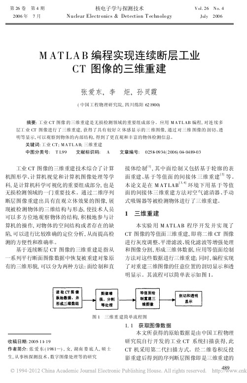
第26卷 第4期核电子学与探测技术V ol.26 N o.42006年 7月Nuclear Electr onics &Detection T echnolo gyJuly 2006M AT LA B 编程实现连续断层工业CT 图像的三维重建张爱东,李 炬,孙灵霞(中国工程物理研究院,四川绵阳621900)摘要:工业CT 图像的三维重建是无损检测领域的重要组成部分。
应用M A T L AB 编程,对连续多层工业CT 图像进行了三维重建,获得了具有较好立体感显示的三维图像,通过对三维图像的剖切、透明等显示,可以观察到物体的内部结构,得到了更直观和丰富的物体检测信息。
关键词:工业CT ;M A T L A B;三维重建中图分类号: T L99 文献标识码: A 文章编号: 0258-0934(2006)04-0489-03收稿日期:2005-11-19作者简介:张爱东(1981)),女,湖南娄底人,硕士生,从事核探测技术、数字图像处理等的研究工业CT 图像的三维重建技术综合了计算机图形学、计算机视觉和计算机图像处理等学科,是计算机科学可视化的重要组成部分,也是无损检测领域的一门重要技术。
通过二维序列断层图像重建出具有直观立体效果的图像,展现被检测物体的三维结构与形态,使技术人员可以多方位地观察物体的结构,积极地参与计算机的操作,对物体的空间结构或者存在的缺陷,可以进行比较准确的定位分析,从而提高检测的方便性和准确率。
基于连续断层CT 图像的三维重建是指从一系列平行断面图像数据中恢复被重建对象原有的三维形貌,可以分为两种方法:面绘制和直接体绘制[1],其中面绘制又包括基于轮廓的表面重建、基于等值面的间接体三维重建[2]等。
本论文是在M AT LAB [3,4]环境下用基于等值面的间接体三维重建方法对空气滤清器、手动式吸锡器等被检测物体进行了三维重建。
1 三维重建本实验用M ATLAB 程序开发并实现了CT 图像的等值面三维重建,即将二维CT 图像进行灰度调整、平滑滤波、锐化滤波等增强处理和图像分割,形成三维体数据,应用等值面绘制方法对这些数据进行三维重建;同时,编程实现了对重建三维图像的任意位置的剖切显示和透明显示。
基于MC-E算法的CT图像三维重建
基于MC-E算法的CT图像三维重建李怡敏; 王宝珠; 刘翠响; 高妍【期刊名称】《《计算机工程与设计》》【年(卷),期】2019(040)010【总页数】5页(P2959-2963)【关键词】移动立方体算法; 三维重建; 医学图像; 二义性; 中值法; 线性插值【作者】李怡敏; 王宝珠; 刘翠响; 高妍【作者单位】河北工业大学信息工程学院天津300401【正文语种】中文【中图分类】TP391.410 引言医学图像,即通过医疗装置测量得到的图像数据,包括由CT(computed tomography)、MRI(magnetic resonance imaging)、PET(positron emission tomography)、SPECT(single photon emission computerized tomography)等各式医学影像设备形成的图像[1]。
为提高医生诊断和治疗方案的准确性,需要从2D的图像断层序列中,重建成具有直观立体效果的3D图像,显示组织、器官及骨骼的三维结构信息。
目前的三维重建算法,主要分为面绘制和体绘制两类[2],面绘制主要是利用各类几何图元,包括三角面片、多边形等,连接起来构造等值面,基于体元绘制等值面的方法有3种较为常见,分别是立方块(Cuberille)算法、移动立方体(marching cubes,MC)算法以及剖分立方体(dividing cubes)算法;体绘制是根据一定的物理模型,直接将体数据绘制成三维模型,常用的算法包括光线投射算法(ray casting,RC)、错切-变形(Shear-Warp)算法、溅射(Sputtering)算法等。
文献[3]通过VTK环境下的仿真实验,使用自带的RC算法对71张肺部CT图像进行了三维重建,来比较几种分割方法的效果。
文献[4]从算法效率、交互性以及重建质量3个方面对面绘制和体绘制中具有代表性的MC算法及RC算法进行了分析比较,体绘制方法虽然在重建效果上更加理想,但是重建过程中,需要处理大量的数据,运算时间长,面绘制虽然效率更高,但只能显示物体表面信息,无法保证体素信息的完整性。
CT图像三维重建(附源码)
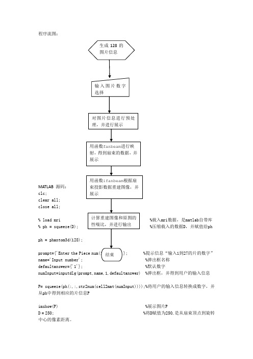
程序流图:MATLAB 源码:clc;clear all;close all;载入mri数据,是matlab自带库压缩载入的数据D,并赋值给ph ph = phantom3d(128);prompt={'Enter the 提示信息“输入1到27的片的数字”弹出框名称defaultanswer={'1'}; %默认数字numInput=inputdlg(prompt,name,1,defaultanswer) %弹出框,并得到用户的输入信息P= squeeze(ph(:,:,str2num(cell2mat(numInput))));%将用户的输入信息转换成数字,并从ph中得到相应的片信息Pimshow(P) %展示图片PD = 250; %将D赋值为250,是从扇束顶点到旋转中心的像素距离。
dsensor1 = 2; %正实数指定扇束传感器的间距2F1 = fanbeam(P,D,'FanSensorSpacing',dsensor1); %通过P,D等计算扇束的数据值dsensor2 = 1; %正实数指定扇束传感器的间距1F2 = fanbeam(P,D,'FanSensorSpacing',dsensor2); %通过P,D等计算扇束的数据值dsensor3 = 0.25 %正实数指定扇束传感器的间距0.25 [F3, sensor_pos3, fan_rot_angles3] = fanbeam(P,D,...'FanSensorSpacing',dsensor3); %通过P,D等计算扇束的数据值,并得到扇束传感器的位置sensor_pos3和旋转角度fan_rot_angles3figure, %创建窗口imagesc(fan_rot_angles3, sensor_pos3, F3) %根据计算出的位置和角度展示F3的图片colormap(hot); %设置色图为hotcolorbar; %显示色栏xlabel('Fan Rotation Angle (degrees)') %定义x坐标轴ylabel('Fan Sensor Position (degrees)') %定义y坐标轴output_size = max(size(P)); %得到P维数的最大值,并赋值给output_sizeIfan1 = ifanbeam(F1,D, ...'FanSensorSpacing',dsensor1,'OutputSize',output_size);%根据扇束投影数据F1及D等数据重建图像figure, imshow(Ifan1) %创建窗口,并展示图片Ifan1title('图一');disp('图一和原图的性噪比为:');result=psnr1(Ifan1,P);Ifan2 = ifanbeam(F2,D, ...'FanSensorSpacing',dsensor2,'OutputSize',output_size);%根据扇束投影数据F2及D等数据重建图像figure, imshow(Ifan2) %创建窗口,并展示图片Ifan2disp('图二和原图的性噪比为:');result=psnr1(Ifan2,P);title('图二');Ifan3 = ifanbeam(F3,D, ...'FanSensorSpacing',dsensor3,'OutputSize',output_size);%根据扇束投影数据F3及D等数据重建图像figure, imshow(Ifan3) %创建窗口,并展示图片Ifan3title('图三');disp('图三和原图的性噪比为:');result=psnr1(Ifan3,P);function [p,ellipse]=phantom3d(varargin)%PHANTOM3D Three-dimensional analogue of MATLAB Shepp-Logan phantom% P = PHANTOM3D(DEF,N) generates a 3D head phantom that can% be used to test 3-D reconstruction algorithms.%% DEF is a string that specifies the type of head phantom to generate.% Valid values are:%% 'Shepp-Logan' A test image used widely by researchers in% tomography% 'Modified Shepp-Logan' (default) A variant of the Shepp-Logan phantom % in which the contrast is improved for better % visual perception.%% N is a scalar that specifies the grid size of P.% If you omit the argument, N defaults to 64.%% P = PHANTOM3D(E,N) generates a user-defined phantom, where each row% of the matrix E specifies an ellipsoid in the image. E has ten columns,% with each column containing a different parameter for the ellipsoids:%% Column 1: A the additive intensity value of the ellipsoid% Column 2: a the length of the x semi-axis of the ellipsoid% Column 3: b the length of the y semi-axis of the ellipsoid% Column 4: c the length of the z semi-axis of the ellipsoid% Column 5: x0 the x-coordinate of the center of the ellipsoid% Column 6: y0 the y-coordinate of the center of the ellipsoid% Column 7: z0 the z-coordinate of the center of the ellipsoid% Column 8: phi phi Euler angle (in degrees) (rotation about z-axis)% Column 9: theta theta Euler angle (in degrees) (rotation about x-axis)% Column 10: psi psi Euler angle (in degrees) (rotation about z-axis)%% For purposes of generating the phantom, the domains for the x-, y-, and% z-axes span [-1,1]. Columns 2 through 7 must be specified in terms% of this range.%% [P,E] = PHANTOM3D(...) returns the matrix E used to generate the phantom.%% Class Support% -------------% All inputs must be of class double. All outputs are of class double.%% Remarks% -------% For any given voxel in the output image, the voxel's value is equal to the% sum of the additive intensity values of all ellipsoids that the voxel is a% part of. If a voxel is not part of any ellipsoid, its value is 0.%% The additive intensity value A for an ellipsoid can be positive or negative;% if it is negative, the ellipsoid will be darker than the surrounding pixels.% Note that, depending on the values of A, some voxels may have values outside % the range [0,1].%% Example% -------% ph = phantom3d(128);% figure, imshow(squeeze(ph(64,:,:)))%% Copyright2005MatthiasChristianSchabel(***************************) % University of Utah Department of Radiology% Utah Center for Advanced Imaging Research% 729 Arapeen Drive% Salt Lake City, UT 84108-1218%% This code is released under the Gnu Public License (GPL). For more information, % see : /copyleft/gpl.html%% Portions of this code are based on phantom.m, copyrighted by the Mathworks %[ellipse,n] = parse_inputs(varargin{:});p = zeros([n n n]);rng = ( (0:n-1)-(n-1)/2 ) / ((n-1)/2);[x,y,z] = meshgrid(rng,rng,rng);coord = [flatten(x); flatten(y); flatten(z)];p = flatten(p);for k = 1:size(ellipse,1)A = ellipse(k,1); % Amplitude change for this ellipsoidasq = ellipse(k,2)^2; % a^2bsq = ellipse(k,3)^2; % b^2csq = ellipse(k,4)^2; % c^2x0 = ellipse(k,5); % x offsety0 = ellipse(k,6); % y offsetz0 = ellipse(k,7); % z offsetphi = ellipse(k,8)*pi/180; % first Euler angle in radianstheta = ellipse(k,9)*pi/180; % second Euler angle in radianspsi = ellipse(k,10)*pi/180; % third Euler angle in radianscphi = cos(phi);sphi = sin(phi);ctheta = cos(theta);stheta = sin(theta);cpsi = cos(psi);spsi = sin(psi);% Euler rotation matrixalpha = [cpsi*cphi-ctheta*sphi*spsi cpsi*sphi+ctheta*cphi*spsi spsi*stheta;-spsi*cphi-ctheta*sphi*cpsi -spsi*sphi+ctheta*cphi*cpsi cpsi*stheta;stheta*sphi -stheta*cphi ctheta];% rotated ellipsoid coordinatescoordp = alpha*coord;idx = find((coordp(1,:)-x0).^2./asq + (coordp(2,:)-y0).^2./bsq + (coordp(3,:)-z0).^2./csq <= 1);p(idx) = p(idx) + A;endp = reshape(p,[n n n]);return;function out = flatten(in)out = reshape(in,[1 prod(size(in))]);return;function [e,n] = parse_inputs(varargin)% e is the m-by-10 array which defines ellipsoids% n is the size of the phantom brain imagen = 128; % The default sizee = [];defaults = {'shepp-logan', 'modified shepp-logan', 'yu-ye-wang'};for i=1:narginif ischar(varargin{i}) % Look for a default phantom def = lower(varargin{i});idx = strmatch(def, defaults);if isempty(idx)eid = sprintf('Images:%s:unknownPhantom',mfilename);msg = 'Unknown default phantom selected.';error(eid,'%s',msg);endswitch defaults{idx}case 'shepp-logan'e = shepp_logan;case 'modified shepp-logan'e = modified_shepp_logan;case 'yu-ye-wang'e = yu_ye_wang;endelseif numel(varargin{i})==1n = varargin{i}; % a scalar is the image size elseif ndims(varargin{i})==2 && size(varargin{i},2)==10e = varargin{i}; % user specified phantomelseeid = sprintf('Images:%s:invalidInputArgs',mfilename);msg = 'Invalid input arguments.';error(eid,'%s',msg);endend% ellipse is not yet definedif isempty(e)e = modified_shepp_logan;endreturn;%%%%%%%%%%%%%%%%%%%%%%%%%%%%%% Default head phantoms: % %%%%%%%%%%%%%%%%%%%%%%%%%%%%%function e = shepp_logane = modified_shepp_logan;e(:,1) = [1 -.98 -.02 -.02 .01 .01 .01 .01 .01 .01];return;function e = modified_shepp_logan%% This head phantom is the same as the Shepp-Logan except% the intensities are changed to yield higher contrast in% the image. Taken from Toft, 199-200.%% A a b c x0 y0 z0 phi theta psi% -----------------------------------------------------------------e = [ 1 .6900 .920 .810 0 0 0 0 0 0-.8 .6624 .874 .780 0 -.0184 0 0 0 0-.2 .1100 .310 .220 .22 0 0 -18 0 10-.2 .1600 .410 .280 -.22 0 0 18 0 10.1 .2100 .250 .410 0 .35 -.15 0 0 0.1 .0460 .046 .050 0 .1 .25 0 0 0.1 .0460 .046 .050 0 -.1 .25 0 0 0.1 .0460 .023 .050 -.08 -.605 0 0 0 0.1 .0230 .023 .020 0 -.606 0 0 0 0.1 .0230 .046 .020 .06 -.605 0 0 0 0 ]; return;function e = yu_ye_wang%% Yu H, Ye Y, Wang G, Katsevich-Type Algorithms for Variable Radius Spiral Cone-Beam CT%% A a b c x0 y0 z0 phi theta psi% -----------------------------------------------------------------e = [ 1 .6900 .920 .900 0 0 0 0 0 0-.8 .6624 .874 .880 0 0 0 0 0 0-.2 .4100 .160 .210 -.22 0 -.25 108 0 0-.2 .3100 .110 .220 .22 0 -.25 72 0 0.2 .2100 .250 .500 0 .35 -.25 0 0 0.2 .0460 .046 .046 0 .1 -.25 0 0 0.1 .0460 .023 .020 -.08 -.65 -.25 0 0 0.1 .0460 .023 .020 .06 -.65 -.25 90 0 0.2 .0560 .040 .100 .06 -.105 .625 90 0 0-.2 .0560 .056 .100 0 .100 .625 0 0 0 ];return;% func——计算两幅图像的psnr值function result=psnr1(in1,in2)z=mse(in1,in2);result=10*log10(255.^2/z)% plot(result)function z=mse(x,y)if ndims(x)==3x=rgb2gray(x);endif ndims(y)==3y=rgb2gray(y);endx=double(x);y=double(y);[m1,n1]=size(x);[m2,n2]=size(y);m=min(m1,m2);n=min(n1,n2);z=0;for i=1:mfor j=1:nz=z+(x(i,j)-y(i,j)).^2;endendz=z/(m*n);。
三维重建学习记录2-将CT数据集转化为三维模型

三维重建学习记录2-将CT数据集转化为三维模型软件:VS2017+VTK8.2先上代码:1#define vtkRenderingCore_AUTOINIT 3(vtkInteractionStyle,vtkRenderingFreeType,vtkRenderingOpenGL2)2#define vtkRenderingVolume_AUTOINIT 1(vtkRenderingVolumeOpenGL2)3 #include "vtkDICOMImageReader.h"4 #include "vtkRenderWindowInteractor.h"5 #include "vtkRenderer.h"6 #include "vtkRenderWindow.h"7 #include "vtkMarchingCubes.h"8 #include "vtkStripper.h"9 #include "vtkActor.h"10 #include "vtkPolyDataMapper.h"11 #include "vtkProperty.h"12 #include "vtkCamera.h"13 #include "vtkBoxWidget.h"14 #include "vtkSmartPointer.h"15 #include "vtkTriangleFilter.h"16 #include "vtkMassProperties.h"17 #include "vtkSmoothPolyDataFilter.h"18 #include "vtkPolyDataNormals.h"19 #include "vtkContourFilter.h"20 #include "vtkRecursiveDividingCubes.h"21 #include "vtkSTLWriter.h"2223int main(int argc, char* argv[])24 {25 std::string filename = "out_Smooth.stl";//设置输出⽂件路径2627//读取⼆维切⽚数据序列28 vtkSmartPointer< vtkDICOMImageReader >reader =29 vtkSmartPointer< vtkDICOMImageReader >::New();30 reader->SetDataByteOrderToLittleEndian();31 reader->SetDirectoryName("E://dicomimage");//设置读取路径3233 reader->SetDataSpacing(1.0, 1.0, 1.0);//设置每个体素的⼤⼩34 reader->Update();353637//抽取等值⾯为⾻头的信息38//MC算法39 vtkSmartPointer< vtkMarchingCubes > boneExtractor =40 vtkSmartPointer< vtkMarchingCubes >::New();41 boneExtractor->SetInputConnection(reader->GetOutputPort());42 boneExtractor->SetValue(0, 400); //设置提取的等值信息43 boneExtractor->Update();444546//利⽤ContourFilter提取等值⾯47/*vtkSmartPointer< vtkContourFilter > boneExtractor =48 vtkSmartPointer< vtkContourFilter >::New();49 boneExtractor->SetInputConnection(reader->GetOutputPort());50 boneExtractor->SetValue(0, 200); //设置提取的等值信息51 boneExtractor->Update();*/5253//DC算法耗时长,模型有明显缝隙54/*vtkSmartPointer< vtkRecursiveDividingCubes > boneExtractor =55 vtkSmartPointer< vtkRecursiveDividingCubes >::New();56 boneExtractor->SetInputConnection(reader->GetOutputPort());57 boneExtractor->SetValue(500);58 boneExtractor->SetDistance(1);59 boneExtractor->SetIncrement(2);60 boneExtractor->Update();*/61626364//剔除旧的或废除的数据单元,提⾼绘制速度(可略去这⼀步)65 vtkSmartPointer< vtkStripper > boneStripper =66 vtkSmartPointer< vtkStripper >::New(); //三⾓带连接67 boneStripper->SetInputConnection(boneExtractor->GetOutputPort());68 boneStripper->Update();6970//平滑滤波71 vtkSmartPointer<vtkSmoothPolyDataFilter> pSmoothPolyDataFilter = vtkSmartPointer<vtkSmoothPolyDataFilter>::New();72 pSmoothPolyDataFilter->SetInputConnection(boneStripper->GetOutputPort());73//pSmoothPolyDataFilter->SetNumberOfIterations(m_nNumberOfIterations);74 pSmoothPolyDataFilter->SetRelaxationFactor(0.05);7576 vtkSmartPointer<vtkPolyDataNormals> pPolyDataNormals = vtkSmartPointer<vtkPolyDataNormals>::New();77 pPolyDataNormals->SetInputConnection(pSmoothPolyDataFilter->GetOutputPort());78//pPolyDataNormals->SetFeatureAngle(m_nFeatureAngle);798081//将模型输出到⼊STL⽂件82 vtkSmartPointer<vtkSTLWriter> stlWriter =83 vtkSmartPointer<vtkSTLWriter>::New();84 stlWriter->SetFileName(filename.c_str());85 stlWriter->SetInputConnection(pPolyDataNormals->GetOutputPort());86 stlWriter->Write();878889//建⽴映射90 vtkSmartPointer< vtkPolyDataMapper > boneMapper =91 vtkSmartPointer< vtkPolyDataMapper >::New();92 boneMapper->SetInputData(pPolyDataNormals->GetOutput());93 boneMapper->ScalarVisibilityOff();94//建⽴⾓⾊95 vtkSmartPointer< vtkActor > bone =96 vtkSmartPointer< vtkActor >::New();97 bone->SetMapper(boneMapper);9899 bone->GetProperty()->SetDiffuseColor(1.0, 1.0, 1.0);100 bone->GetProperty()->SetSpecular(.3);101 bone->GetProperty()->SetSpecularPower(20);102103//定义绘制器104 vtkSmartPointer< vtkRenderer > aRenderer =105 vtkSmartPointer< vtkRenderer >::New();106//定义绘制窗⼝107 vtkSmartPointer< vtkRenderWindow > renWin =108 vtkSmartPointer< vtkRenderWindow >::New();109 renWin->AddRenderer(aRenderer);110//定义窗⼝交互器111 vtkSmartPointer< vtkRenderWindowInteractor > iren =112 vtkSmartPointer< vtkRenderWindowInteractor >::New();113 iren->SetRenderWindow(renWin);114115//创建⼀个camera116 vtkSmartPointer< vtkCamera > aCamera =117 vtkSmartPointer< vtkCamera >::New();118 aCamera->SetViewUp(0, 0, -1);119 aCamera->SetPosition(0, 1, 0);120 aCamera->SetFocalPoint(0, 0, 0);121122 aRenderer->AddActor(bone);123 aRenderer->SetActiveCamera(aCamera);124 aRenderer->ResetCamera();125 aCamera->Dolly(1.5);126 aRenderer->SetBackground(0, 0, 0);127 aRenderer->ResetCameraClippingRange();128129//将3D模型渲染到绘制窗⼝130 iren->Initialize();131 iren->Start();132133return0;134 }View Code注:运⾏后笔记本要等⼏分钟,等待渲染完成。
CT重建
CTVE利用Navigator smooth软件 (GE),Voyager软件(Picker),Fly软件 (Simens)对空腔器官内表面具有相同体 素值范围的部分进行三维表面重建而产 生立体图像,CT值设定为完全透明状态, 透过度(Transparency)为100%。 再利用计算机的模拟导航技术(飞越 方式,漫游技术fly-through sequence 功能键)进行腔内观察。
SSD三维重建清晰显示脊椎解剖关 系
手掌骨结构SSD
正常肝脾及其血管SSD
4
表面透视成像(RaySum)
或仿真透视、透明显示、透明投影(Raysumprojection RSP) 、 CT透明重建、也称空气投影 成像(air cast imaging ACI) 是GE公司开发的一种透明显示方式,是在SSD 三维重建图像的基础上用RaySum软件使空腔脏器图 像透明,以观察空腔脏器内和腔壁的情况,如同进 行“透视”。即不仅能观察到面向观察者的胃、肠 壁,同时视线能穿透前层胃壁或肠壁观察到后层胃、 肠。 主要用于气管、支气管、胃肠道、血管、胆囊、 胆道、输尿管、膀胱等空腔脏器的成像。
最大强度投影法(MIP)或最大密度投影 法,亦称最强象素投影法(MaximumPixel-Intensity Projection)、最大信 号强度投影法或最强信号投影法
最大密度投影法(MIP)图象
是通过计算机将重建范围内各条射线 上具有最大CT值的象素集合二维显示,而 将密度低的组织结构尽可能除掉。 经过MIP处理后感兴趣的解剖结构的位 置、形状、坐标等能够清晰再现,可以重 建类似X线造影的图像。并可多平面、多角 度、不同厚度观察。
也可以根据轴位和多平面重组(MPR) 图像确定视点(光标)的位置和观察方向, 分别从头侧或足侧进行腔内观察。 再赋予人工伪色彩和不同的光照强 度,最后用电影形式(move loop mode) 以15-30幀/s的速度连续依此回放。 即可获得类似纤维内窥镜进行和直 视观察效果的动态重建图像。
- 1、下载文档前请自行甄别文档内容的完整性,平台不提供额外的编辑、内容补充、找答案等附加服务。
- 2、"仅部分预览"的文档,不可在线预览部分如存在完整性等问题,可反馈申请退款(可完整预览的文档不适用该条件!)。
- 3、如文档侵犯您的权益,请联系客服反馈,我们会尽快为您处理(人工客服工作时间:9:00-18:30)。
程序流图:MATLAB 源码:clc;clear all;close all;载入mri数据,是matlab自带库压缩载入的数据D,并赋值给ph ph = phantom3d(128);prompt={'Enter the 提示信息“输入1到27的片的数字”弹出框名称defaultanswer={'1'}; %默认数字numInput=inputdlg(prompt,name,1,defaultanswer) %弹出框,并得到用户的输入信息P= squeeze(ph(:,:,str2num(cell2mat(numInput))));%将用户的输入信息转换成数字,并从ph中得到相应的片信息Pimshow(P) %展示图片PD = 250; %将D赋值为250,是从扇束顶点到旋转中心的像素距离。
dsensor1 = 2; %正实数指定扇束传感器的间距2F1 = fanbeam(P,D,'FanSensorSpacing',dsensor1); %通过P,D等计算扇束的数据值dsensor2 = 1; %正实数指定扇束传感器的间距1F2 = fanbeam(P,D,'FanSensorSpacing',dsensor2); %通过P,D等计算扇束的数据值dsensor3 = 0.25 %正实数指定扇束传感器的间距0.25 [F3, sensor_pos3, fan_rot_angles3] = fanbeam(P,D,...'FanSensorSpacing',dsensor3); %通过P,D等计算扇束的数据值,并得到扇束传感器的位置sensor_pos3和旋转角度fan_rot_angles3figure, %创建窗口imagesc(fan_rot_angles3, sensor_pos3, F3) %根据计算出的位置和角度展示F3的图片colormap(hot); %设置色图为hotcolorbar; %显示色栏xlabel('Fan Rotation Angle (degrees)') %定义x坐标轴ylabel('Fan Sensor Position (degrees)') %定义y坐标轴output_size = max(size(P)); %得到P维数的最大值,并赋值给output_sizeIfan1 = ifanbeam(F1,D, ...'FanSensorSpacing',dsensor1,'OutputSize',output_size);%根据扇束投影数据F1及D等数据重建图像figure, imshow(Ifan1) %创建窗口,并展示图片Ifan1title('图一');disp('图一和原图的性噪比为:');result=psnr1(Ifan1,P);Ifan2 = ifanbeam(F2,D, ...'FanSensorSpacing',dsensor2,'OutputSize',output_size);%根据扇束投影数据F2及D等数据重建图像figure, imshow(Ifan2) %创建窗口,并展示图片Ifan2disp('图二和原图的性噪比为:');result=psnr1(Ifan2,P);title('图二');Ifan3 = ifanbeam(F3,D, ...'FanSensorSpacing',dsensor3,'OutputSize',output_size);%根据扇束投影数据F3及D等数据重建图像figure, imshow(Ifan3) %创建窗口,并展示图片Ifan3title('图三');disp('图三和原图的性噪比为:');result=psnr1(Ifan3,P);function [p,ellipse]=phantom3d(varargin)%PHANTOM3D Three-dimensional analogue of MATLAB Shepp-Logan phantom% P = PHANTOM3D(DEF,N) generates a 3D head phantom that can% be used to test 3-D reconstruction algorithms.%% DEF is a string that specifies the type of head phantom to generate.% Valid values are:%% 'Shepp-Logan' A test image used widely by researchers in% tomography% 'Modified Shepp-Logan' (default) A variant of the Shepp-Logan phantom % in which the contrast is improved for better % visual perception.%% N is a scalar that specifies the grid size of P.% If you omit the argument, N defaults to 64.%% P = PHANTOM3D(E,N) generates a user-defined phantom, where each row% of the matrix E specifies an ellipsoid in the image. E has ten columns,% with each column containing a different parameter for the ellipsoids:%% Column 1: A the additive intensity value of the ellipsoid% Column 2: a the length of the x semi-axis of the ellipsoid% Column 3: b the length of the y semi-axis of the ellipsoid% Column 4: c the length of the z semi-axis of the ellipsoid% Column 5: x0 the x-coordinate of the center of the ellipsoid% Column 6: y0 the y-coordinate of the center of the ellipsoid% Column 7: z0 the z-coordinate of the center of the ellipsoid% Column 8: phi phi Euler angle (in degrees) (rotation about z-axis)% Column 9: theta theta Euler angle (in degrees) (rotation about x-axis)% Column 10: psi psi Euler angle (in degrees) (rotation about z-axis)%% For purposes of generating the phantom, the domains for the x-, y-, and% z-axes span [-1,1]. Columns 2 through 7 must be specified in terms% of this range.%% [P,E] = PHANTOM3D(...) returns the matrix E used to generate the phantom.%% Class Support% -------------% All inputs must be of class double. All outputs are of class double.%% Remarks% -------% For any given voxel in the output image, the voxel's value is equal to the% sum of the additive intensity values of all ellipsoids that the voxel is a% part of. If a voxel is not part of any ellipsoid, its value is 0.%% The additive intensity value A for an ellipsoid can be positive or negative;% if it is negative, the ellipsoid will be darker than the surrounding pixels.% Note that, depending on the values of A, some voxels may have values outside % the range [0,1].%% Example% -------% ph = phantom3d(128);% figure, imshow(squeeze(ph(64,:,:)))%% Copyright2005MatthiasChristianSchabel(***************************) % University of Utah Department of Radiology% Utah Center for Advanced Imaging Research% 729 Arapeen Drive% Salt Lake City, UT 84108-1218%% This code is released under the Gnu Public License (GPL). For more information, % see : /copyleft/gpl.html%% Portions of this code are based on phantom.m, copyrighted by the Mathworks %[ellipse,n] = parse_inputs(varargin{:});p = zeros([n n n]);rng = ( (0:n-1)-(n-1)/2 ) / ((n-1)/2);[x,y,z] = meshgrid(rng,rng,rng);coord = [flatten(x); flatten(y); flatten(z)];p = flatten(p);for k = 1:size(ellipse,1)A = ellipse(k,1); % Amplitude change for this ellipsoidasq = ellipse(k,2)^2; % a^2bsq = ellipse(k,3)^2; % b^2csq = ellipse(k,4)^2; % c^2x0 = ellipse(k,5); % x offsety0 = ellipse(k,6); % y offsetz0 = ellipse(k,7); % z offsetphi = ellipse(k,8)*pi/180; % first Euler angle in radianstheta = ellipse(k,9)*pi/180; % second Euler angle in radianspsi = ellipse(k,10)*pi/180; % third Euler angle in radianscphi = cos(phi);sphi = sin(phi);ctheta = cos(theta);stheta = sin(theta);cpsi = cos(psi);spsi = sin(psi);% Euler rotation matrixalpha = [cpsi*cphi-ctheta*sphi*spsi cpsi*sphi+ctheta*cphi*spsi spsi*stheta;-spsi*cphi-ctheta*sphi*cpsi -spsi*sphi+ctheta*cphi*cpsi cpsi*stheta;stheta*sphi -stheta*cphi ctheta];% rotated ellipsoid coordinatescoordp = alpha*coord;idx = find((coordp(1,:)-x0).^2./asq + (coordp(2,:)-y0).^2./bsq + (coordp(3,:)-z0).^2./csq <= 1);p(idx) = p(idx) + A;endp = reshape(p,[n n n]);return;function out = flatten(in)out = reshape(in,[1 prod(size(in))]);return;function [e,n] = parse_inputs(varargin)% e is the m-by-10 array which defines ellipsoids% n is the size of the phantom brain imagen = 128; % The default sizee = [];defaults = {'shepp-logan', 'modified shepp-logan', 'yu-ye-wang'};for i=1:narginif ischar(varargin{i}) % Look for a default phantom def = lower(varargin{i});idx = strmatch(def, defaults);if isempty(idx)eid = sprintf('Images:%s:unknownPhantom',mfilename);msg = 'Unknown default phantom selected.';error(eid,'%s',msg);endswitch defaults{idx}case 'shepp-logan'e = shepp_logan;case 'modified shepp-logan'e = modified_shepp_logan;case 'yu-ye-wang'e = yu_ye_wang;endelseif numel(varargin{i})==1n = varargin{i}; % a scalar is the image size elseif ndims(varargin{i})==2 && size(varargin{i},2)==10e = varargin{i}; % user specified phantomelseeid = sprintf('Images:%s:invalidInputArgs',mfilename);msg = 'Invalid input arguments.';error(eid,'%s',msg);endend% ellipse is not yet definedif isempty(e)e = modified_shepp_logan;endreturn;%%%%%%%%%%%%%%%%%%%%%%%%%%%%%% Default head phantoms: % %%%%%%%%%%%%%%%%%%%%%%%%%%%%%function e = shepp_logane = modified_shepp_logan;e(:,1) = [1 -.98 -.02 -.02 .01 .01 .01 .01 .01 .01];return;function e = modified_shepp_logan%% This head phantom is the same as the Shepp-Logan except% the intensities are changed to yield higher contrast in% the image. Taken from Toft, 199-200.%% A a b c x0 y0 z0 phi theta psi% -----------------------------------------------------------------e = [ 1 .6900 .920 .810 0 0 0 0 0 0-.8 .6624 .874 .780 0 -.0184 0 0 0 0-.2 .1100 .310 .220 .22 0 0 -18 0 10-.2 .1600 .410 .280 -.22 0 0 18 0 10.1 .2100 .250 .410 0 .35 -.15 0 0 0.1 .0460 .046 .050 0 .1 .25 0 0 0.1 .0460 .046 .050 0 -.1 .25 0 0 0.1 .0460 .023 .050 -.08 -.605 0 0 0 0.1 .0230 .023 .020 0 -.606 0 0 0 0.1 .0230 .046 .020 .06 -.605 0 0 0 0 ]; return;function e = yu_ye_wang%% Yu H, Ye Y, Wang G, Katsevich-Type Algorithms for Variable Radius Spiral Cone-Beam CT%% A a b c x0 y0 z0 phi theta psi% -----------------------------------------------------------------e = [ 1 .6900 .920 .900 0 0 0 0 0 0-.8 .6624 .874 .880 0 0 0 0 0 0-.2 .4100 .160 .210 -.22 0 -.25 108 0 0-.2 .3100 .110 .220 .22 0 -.25 72 0 0.2 .2100 .250 .500 0 .35 -.25 0 0 0.2 .0460 .046 .046 0 .1 -.25 0 0 0.1 .0460 .023 .020 -.08 -.65 -.25 0 0 0.1 .0460 .023 .020 .06 -.65 -.25 90 0 0.2 .0560 .040 .100 .06 -.105 .625 90 0 0-.2 .0560 .056 .100 0 .100 .625 0 0 0 ];return;% func——计算两幅图像的psnr值function result=psnr1(in1,in2)z=mse(in1,in2);result=10*log10(255.^2/z)% plot(result)function z=mse(x,y)if ndims(x)==3x=rgb2gray(x);endif ndims(y)==3y=rgb2gray(y);endx=double(x);y=double(y);[m1,n1]=size(x);[m2,n2]=size(y);m=min(m1,m2);n=min(n1,n2);z=0;for i=1:mfor j=1:nz=z+(x(i,j)-y(i,j)).^2;endendz=z/(m*n);。