东南大学数学建模试卷+答案
数学建模竞赛参考答案

数学建模竞赛参考答案数学建模竞赛参考答案数学建模竞赛是一项旨在培养学生综合运用数学知识和解决实际问题能力的竞赛活动。
参赛者需要通过分析问题、建立数学模型、求解问题等环节,最终给出合理的答案和解决方案。
在这篇文章中,我们将为大家提供一些数学建模竞赛的参考答案,希望能够给参赛者们提供一些启示和帮助。
第一题:某公司的销售额预测问题描述:某公司希望通过过去几年的销售数据,预测未来一年的销售额。
请根据给定的销售数据,建立合适的数学模型,并给出未来一年的销售额预测值。
解答思路:根据问题描述,我们可以将销售额看作是时间的函数,即销售额随时间变化。
可以使用回归分析的方法来建立数学模型。
首先,我们将销售额作为因变量,时间作为自变量,通过拟合曲线来预测未来一年的销售额。
我们可以选择多项式回归模型来拟合曲线。
通过将时间作为自变量,销售额作为因变量,进行多项式回归分析,可以得到一个多项式函数,该函数可以描述销售额随时间变化的趋势。
然后,我们可以使用该多项式函数来预测未来一年的销售额。
将未来一年的时间代入多项式函数中,即可得到未来一年的销售额预测值。
第二题:城市交通流量优化问题描述:某城市的交通流量问题日益突出,如何优化交通流量成为了当地政府亟待解决的难题。
请根据给定的交通数据和道路拓扑结构,建立合适的数学模型,并给出交通流量优化的方案。
解答思路:根据问题描述,我们可以将城市的交通流量看作是网络中的流量分配问题。
可以使用网络流模型来建立数学模型。
首先,我们需要将城市的道路网络抽象成一个有向图,节点表示交叉口,边表示道路,边上的权值表示道路的容量。
然后,我们可以使用最小费用最大流算法来求解交通流量优化的方案。
该算法可以通过调整道路上的流量分配,使得整个网络中的流量达到最大,同时满足道路容量的限制。
通过计算最小费用最大流,可以得到交通流量优化的方案。
最后,我们可以根据最小费用最大流算法的结果,对交通流量进行合理调控。
例如,可以调整信号灯的时长,优化交通信号控制系统,减少交通拥堵现象,提高交通效率。
东南大学数学建模试卷10-11-2A做

东 南 大 学 考 试 卷(A 卷)课程名称 数学建模与数学实验 考试学期 2010-2011-2 得分 适用专业 各专业 考试形式 闭卷 考试时间长度 120分钟 (考试可带计算器) 所有数值结果精度要求为保留小数点后两位 一.填空题:(每题2分,共10分) 1. 用Matlab 做AHP 数学实验,常用的命令有 , 等等。
2. 矩阵A 关于模36可逆的充要条件是: 。
3. 泛函332230()()2()3J x x t t x t t dt ⎡⎤=++⎣⎦⎰&取极值的必要条件为 。
4. 请补充一致矩阵缺失的元素136A ⎛⎫ ⎪= ⎪ ⎪⎝⎭。
5. 请列出本人提交的上机实验内容(标题即可) 。
二.选择题:(每题2分,共10分) 1. 在下列Leslie 矩阵中,能保证主特征值唯一的是 ( ) A. 0230.20000.40⎛⎫ ⎪ ⎪ ⎪⎝⎭; B. 0 1.200.10000.30⎛⎫ ⎪ ⎪ ⎪⎝⎭; C. 0070.30000.10⎛⎫ ⎪ ⎪ ⎪⎝⎭; D.以上都对 2. 下列论述正确的是 ( ) A.判断矩阵一定是一致矩阵 B.正互反矩阵一定是判断矩阵 C.能通过一致性检验的矩阵是一致矩阵 D.一致矩阵一定能通过一致性检验 3. n 阶Leslie 矩阵有 个零元素。
( )A.不超过2(1)n -;B.不少于2(1)n -;C.恰好2(1)n -;D.恰好21n -4. Matlab 软件内置命令不可以 ( )A.求矩阵的主特征值B. 做曲线拟合;C. 求解整数线性规划D. 求样条插值函数5. 关于等周问题,下面的描述不正确的有 ( )A.目标泛函可以表示为最简泛函;B.条件泛函为最简泛函;C.条件泛函取值为常数;D. 函数在区间两个端点处可以取任意值三.判断题(每题2分,共10分)1. 马氏链模型中,矩阵一定有特征值1。
( )2. 插值函数不要求通过样本数据点。
《专题 数学建模与数学探究》试卷及答案_高中数学选择性必修 第一册_苏教版_2024-2025学年

《专题数学建模与数学探究》试卷(答案在后面)一、单选题(本大题有8小题,每小题5分,共40分)1、答案:B解析:在数学建模中,对于给定的实际问题,通过建立数学模型来解决问题的方法属于哪种类型?A. 线性规划B. 非线性规划C. 概率统计D. 图论2、答案:C2、某公司生产某种产品,已知生产该产品的成本函数为(C(x)=50x+1000)(单位:元),其中(x)表示生产数量(单位:个)。
若该公司希望将每件产品的售价定为成本加成30%,则为了确保公司的总利润不低于1500元,至少需要生产多少件产品?A. 50B. 60C. 70D. 803、某地气温随时间变化的规律可以用函数(T(t)=−0.2t2+4t+15)来描述,其中(T)表示温度(℃),(t)表示时间(小时)。
若从上午9点开始测量,则到中午12点时,该地的平均温度是多少?A. 21.5℃B. 22℃C. 22.5℃4、某公司为了研究某种产品的销售情况,收集了过去一年的月销售额数据,并通过线性回归模型预测未来几个月的销售额。
若已知过去12个月的月销售额分别为10万元、12万元、15万元、18万元、20万元、23万元、26万元、29万元、32万元、35万元、38万元、40万元。
利用这些数据训练得到的线性回归方程为(y=1.5x+5),其中(x)代表月份,(y)代表销售额(单位:万元)。
请问,根据该模型预测,第13个月的销售额预计是多少?A. 41万元 B) 42万元 C) 43万元 D) 44万元5、某商店为了预测某种商品的需求量,收集了过去几年该商品的销售数据,发现其销售量y与时间x(年份)之间存在线性关系,经过分析得出回归方程为(y=100+5x)。
若预测2023年的销售量,则预计销售量为:A. 600 B) 700 C) 800 D) 9006、某工厂生产一种产品,其成本函数为(C(x)=200+5x)元,其中(x)是生产的数量。
若该工厂希望以每件产品(30)元的价格销售,为了保证不亏本,至少需要生产多少件产品?A. 40 件B. 50 件C. 60 件D. 70 件7、一辆汽车在平直公路上匀速行驶,若该汽车的功率为P,行驶速度为v,则根据公式P=mvv(m为汽车质量,v为速度),可以计算出汽车所受阻力f的大小为()。
数学建模试卷A参考答案
数学建模试卷(A )卷参考答案一、答:二、解:对应的约束条件代表的区域为如下图中阴影部分:两线的交点坐标为()()12,6,4x x =,由图可知z 值在交点处最大,即max 36z =。
三、解:设z 为利润,123,,x x x 分别表示,,A B C 生产的件数,123,,y y y 分别表示,,A B C 生产是否生产(为0-1变量,0表示不生产,1表示生产)。
则 目标函数:()()()123112233max 200025003000300503208040070z y y y y x y x y x =+++-+-+-约束条件:1231231231231232350024000350000,0,0;,0 1;x x x x x x x x x x x x y y or ++≤⎧⎪++≤⎪⎨++≤⎪⎪≥≥≥=⎩四、解:(一)(二)目标层准则层方案层11/2433217551/41/711/21/31/31/52111/31/5311A ⎡⎤⎢⎥⎢⎥⎢⎥=⎢⎥⎢⎥⎢⎥⎣⎦1(),0,ij n n ij ji ijA a a a a ⨯=>=层次分析法的基本步骤成对比较阵和权向量元素之间两两对比,对比采用相对尺度设要比较各准则C 1,C 2,… , C n 对目标O 的重要性:i j ijC C a ⇒A ~成对比较阵 A 是正互反阵要由A 确定C 1,… , C n 对O 的权向量选择旅游地(三)111122221212n n n n n n w w w w w w w w w w w w A w w w w w w ⎡⎤⎢⎥⎢⎥⎢⎥⎢⎥=⎢⎥⎢⎥⎢⎥⎢⎥⎢⎥⎣⎦⎤⎥⎢⎥⎢⎥⎣⎦23a =一致比较允许不一致,但要确定不一致的允许范围考察完全一致的情况12(1),,nW w w w =⇒/ij i ja w w =令12(,,)~T n w w w w =权向量“选择旅游地”中准则层对目标的权向量及一致性检验11/2433217551/41/711/21/31/31/52111/31/5311A ⎡⎤⎢⎥⎢⎥⎢⎥=⎢⎥⎢⎥⎢⎥⎣⎦准则层对目标的成对比较阵最大特征根λ=5.073权向量(特征向量)w =(0.263,0.475,0.055,0.090,0.110)T 5.07350.01851CI -==-一致性指标随机一致性指标 RI=1.12 (查表) 一致性比率CR =0.018/1.12=0.016<0.1通过一致性检验五、解:()221max ni i i a bx y =+-∑,对,a b 分别求偏导数,可以求解得0.9726,0.0500b a ==。
数学建模竞赛 参考答案

数学建模竞赛参考答案数学建模竞赛参考答案数学建模竞赛是一项旨在培养学生数学建模能力和创新思维的竞赛活动。
参赛者需要在规定的时间内,针对给定的问题,运用数学知识和方法进行建模、分析和求解。
本文将为大家提供一些数学建模竞赛的参考答案,希望对参赛者有所帮助。
一、问题一:汽车油耗模型该问题要求建立一个汽车油耗模型,预测在不同的驾驶条件下,汽车的油耗情况。
首先,我们需要收集一些相关的数据,如汽车的型号、发动机排量、行驶里程、驾驶时间、驾驶速度等。
然后,我们可以使用多元线性回归模型来建立汽车油耗模型。
模型的建立如下:油耗= β0 + β1 * 发动机排量+ β2 * 行驶里程+ β3 * 驾驶时间+ β4 * 驾驶速度其中,β0、β1、β2、β3、β4为待求系数。
我们可以使用最小二乘法来估计这些系数。
通过对收集到的数据进行拟合,可以得到最优的系数估计值,并进一步预测不同驾驶条件下的汽车油耗情况。
二、问题二:物流配送路径规划该问题要求设计一个物流配送路径规划模型,以最小化配送成本和时间。
首先,我们需要收集一些相关的数据,如物流中心的位置、客户的位置、货物的重量和体积、道路交通情况等。
然后,我们可以使用网络流模型来建立物流配送路径规划模型。
模型的建立如下:目标函数:最小化总配送成本和时间约束条件:1. 每个客户都必须被配送到,并且每个物流中心只能配送给特定的客户。
2. 配送路径必须满足道路交通规则和限制条件。
3. 货物的重量和体积必须满足配送车辆的载重和容量限制。
我们可以使用线性规划或整数规划方法来求解该模型。
通过对收集到的数据进行建模和求解,可以得到最优的物流配送路径规划方案,以实现最小化成本和时间的目标。
三、问题三:疫情传播模型该问题要求建立一个疫情传播模型,预测疫情在不同地区的传播情况。
首先,我们需要收集一些相关的数据,如人口数量、人口流动情况、疫情传染率、潜伏期、治愈率等。
然后,我们可以使用传染病传播模型来建立疫情传播模型。
数学建模答案(完整版)
1 建立一个命令M 文件:求数60.70.80,权数分别为1.1,1.3,1.2的加权平均数。
在指令窗口输入指令edit ,打开空白的M 文件编辑器;里面输入s=60*1.1+70*1.3+80*1.2;ave=s/3然后保存即可2 编写函数M 文件SQRT.M;函数 x=567.889与0.0368处的近似值(保留有()f x =效数四位)在指令窗口输入指令edit ,打开空白的M 文件编辑器;里面输入syms x1 x2 s1 s2 zhi1 zhi2 x1=567.889;x2=0.368;s1=sqrt(x1);s2=sqrt(x2);zhi1=vpa(s1,4)zhi2=vpa(s2,4)然后保存并命名为SQRT.M 即可3用matlab 计算的值,其中a=2.3,b=4.89.()f x >> syms a b >> a=2.3;b=4.89;>> sqrt(a^2+b^2)/abs(a-b)ans = 2.08644用matlab 计算函数在x=处的值.()f x =3π>> syms x >> x=pi/3;>> sqrt(sin(x)+cos(x))/abs(1-x^2)ans = 12.09625用matlab 计算函数在x=1.23处的值.()arctan f x x =+>> syms x >> x=1.23;>> atan(x)+sqrt(log(x+1))ans = 1.78376 用matlab 计算函数在x=-2.1处的值.()()f x f x ==>> syms x >> x=-2.1;>> 2-3^x*log(abs(x))ans =1.92617 用蓝色.点连线.叉号绘制函数在[0,2]上步长为0.1的图像.>> syms x y>> x=0:0.2:2;y=2*sqrt(x);>> plot(x,y,'b.-')8 用紫色.叉号.实连线绘制函数在上步长为0.2的图像.ln 10y x =+[20,15]-->> syms x y>> x=-20:0.2:-15;y=log(abs(x+10));>> plot(x,y,'mx-')ln 10[20,y x =+--9 用红色.加号连线 虚线绘制函数在[-10,10]上步长为0.2的图像.sin(22x y π=->> syms x y;>> x=-10:0.2:10;y=sin(x/2-pi/2);>> plot(x,y,'r+--')10用紫红色.圆圈.点连线绘制函数在上步长为0.2的图像.sin(2)3y x π=+[0,4]πsin(2)sin()[0,4]322x y x y πππ=+=->> syms x y >> x=0:0.2:4*pi;y=sin(2*x+pi/3);>> plot(x,y,'mo-.')11 在同一坐标中,用分别青色.叉号.实连线与红色.星色.虚连线绘制y=与.y =>> syms x y1 y2>> x=0:pi/50:2*pi;y1=cos(3*sqrt(x));y2=3*cos(sqrt(x));>> plot(x,y1,'cx-',x,y2,'r*--')12 在同一坐标系中绘制函数这三条曲线的图标,并要求用两种方法加234,,y x y x y x ===各种标注.234,,y x y x y x ===>> syms x y1 y2 y3;>> x=-2:0.1:2;y1=x.^2;y2=x.^3;y3=x.^4;plot(x,y1,x,y2,x,y3);13 作曲线的3维图像2sin x t y t z t ⎧=⎪=⎨⎪=⎩>> syms x y t z >> t=0:1/50:2*pi;>> x=t.^2;y=sin(t);z=t;>> stem3(x,y,z)14 作环面在上的3维图像(1cos )cos (1cos )sin sin x u v y u v z u =+⎧⎪=+⎨⎪=⎩(0,2)(0,2)ππ⨯>> syms x y u v z>> u=0:pi/50:2*pi;v=0:pi/50:2*pi;>>x=(1+cos(u)).*cos(v);y=(1+cos(u)).*sin(v);z=sin(u);>> plot3(x,y,z)15 求极限0lim x +→0lim x +→>> syms x y >> y=sin(2^0.5*x)/sqrt(1-cos(x));>> limit(y,x,0,'right') ans = 216 求极限1201lim (3x x +→>> syms y x >> y=(1/3)^(1/(2*x));>> limit(y,x,0,'right') ans = 017求极限lim x >> syms x y >> y=(x*cos(x))/sqrt(1+x^3);>> limit(y,x,+inf) ans = 018 求极限21lim (1x x x x →+∞+->> syms x y >> y=((x+1)/(x-1))^(2*x);>> limit(y,x,+inf) ans = exp(4)19 求极限01cos 2lim sin x xx x →->> syms x y >> y=(1-cos(2*x))/(x*sin(x));>> limit(y,x,0) ans = 220 求极限 x →>> syms x y >> y=(sqrt(1+x)-sqrt(1-x))/x;>> limit(y,x,0) ans = 121 求极限2221lim 2x x x x x →+∞++-+>> syms x y >> y=(x^2+2*x+1)/(x^2-x+2);>> limit(y,x,+inf) ans = 122 求函数y=的导数5(21)arctan x x -+>> syms x y >> y=(2*x-1)^5+atan(x);>> diff(y) ans = 10*(2*x - 1)^4 + 1/(x^2 + 1)23 求函数y=的导数2tan 1x x y x=+>> syms y x>> y=(x*tan(x))/(1+x^2);>> diff(y)ans =tan(x)/(x^2 + 1) + (x*(tan(x)^2 + 1))/(x^2 + 1) - (2*x^2*tan(x))/(x^2 + 1)^224 求函数的导数3tan x y e x -=>> syms y x >> y=exp^(-3*x)*tan(x)>> y=exp(-3*x)*tan(x) y = exp(-3*x)*tan(x) >> diff(y) ans = exp(-3*x)*(tan(x)^2 + 1) - 3*exp(-3*x)*tan(x)25 求函数y=在x=1的导数22ln sin 2x x π+>> syms x y >> y=(1-x)/(1+x);>> diff(y,x,2) ans = 2/(x + 1)^2 - (2*(x - 1))/(x + 1)^3 >> syms x y >> y=2*log(x)+sin(pi*x/2)^2;>> dxdy=diff(y) dxdy = 2/x + pi*cos((pi*x)/2)*sin((pi*x)/2)zhi=subs(dxdy,1)zhi = 226 求函数y=的二阶导数01cos 2lim sin x x x x →-11x x-+>> syms x y>> y=(1-x)/(1+x);>> diff(y,x,2) ans = 2/(x + 1)^2 - (2*(x - 1))/(x + 1)^327 求函数的导数;>> syms x y >> y=((x-1)^3*(3+2*x)^2/(1+x)^4)^0.2;>> diff(y) ans = (((8*x + 12)*(x - 1)^3)/(x + 1)^4 + (3*(2*x + 3)^2*(x - 1)^2)/(x + 1)^4 - (4*(2*x + 3)^2*(x - 1)^3)/(x + 1)^5)/(5*(((2*x + 3)^2*(x - 1)^3)/(x + 1)^4)^(4/5))28在区间()内求函数的最值.,-∞+∞43()341f x x x =-+>> f='-3*x^4+4*x^3-1';>> [x,y]=fminbnd(f,-inf,inf)x =NaN y = NaN >> f='3*x^4-4*x^3+1';>> [x,y]=fminbnd(f,-inf,inf)x = NaN y = NaN29在区间(-1,5)内求函数发的最值.()(f x x =->> f='(x-1)*x^0.6';>> [x,y]=fminbnd(f,-1,5)x =0.3750y = -0.3470>> >> f='-(x-1)*x^0.6';>> [x,y]=fminbnd(f,-1,5)x = 4.9999y = -10.505930 求不定积分(ln 32sin )x x dx -⎰(ln 32sin )x x dx -⎰>> syms x y >> y=log(3*x)-2*sin(x);>> int(y) ans = 2*cos(x) - x + x*log(3) + x*log(x)31求不定积分2sin x e xdx ⎰>> syms x y>> y=exp(x)*sin(x)^2;>> int(y)ans =-(exp(x)*(cos(2*x) + 2*sin(2*x) - 5))/1032. 求不定积分 >> syms x y >> y=x*atan(x)/(1+x)^0.5;>> int(y)Warning: Explicit integral could not be found. ans = int((x*atan(x))/(x + 1)^(1/2), x)33.计算不定积分2(2cos )x x x e dx --⎰>> syms x y >> y=1/exp(x^2)*(2*x-cos(x));>> int(y)Warning: Explicit integral could not be found. ans = int(exp(-x^2)*(2*x - cos(x)), x)34.计算定积分10(32)xe x dx -+⎰>> syms x y >> y=exp(-x)*(3*x+2);>> int(y,0,1) ans = 5 - 8*exp(-1)10(32)x e x dx -+⎰35.计算定积分0x →120(1)cos x arc xdx+⎰>> syms y x>> y=(x^2+1)*acos(x);>> int(y,0,1)ans =11/936.计算定积分10cos ln(1)x x dx +⎰>> syms x y >> y=(cos(x)*log(x+1));>> int(y,0,1)Warning: Explicit integral could not be found. ans = int(log(x + 1)*cos(x), x == 0..1)37计算广义积分;2122x x dx +∞++-∞⎰>> syms y x >> y=(1/(x^2+2*x+2));>> int(y,-inf,inf) ans = pi 38.计算广义积分;20x dx x e +∞-⎰>> syms x y>> y=x^2*exp(-x);>> int(y,0,+inf)ans =2。
大学数学模型试题及答案

大学数学模型试题及答案一、单项选择题(每题2分,共10分)1. 数学模型的一般步骤不包括以下哪一项?A. 模型准备B. 模型假设C. 模型求解D. 数据分析答案:D2. 在数学建模中,以下哪一项不是模型的分类?A. 确定性模型B. 随机性模型C. 动态模型D. 线性模型答案:D3. 数学模型的建立过程中,以下哪一项是不需要的?A. 收集数据B. 模型假设C. 模型求解D. 编写程序答案:D4. 在数学建模中,以下哪一项是模型验证的主要方法?A. 理论分析B. 实验验证C. 专家评估D. 以上都是答案:D5. 数学模型的最终目的是?A. 解决实际问题B. 获得数学结论C. 发表学术论文D. 展示数学技巧答案:A二、填空题(每题2分,共10分)1. 数学模型的三个基本要素包括______、______和______。
答案:假设、变量、关系2. 模型的分类中,根据模型的确定性与否,可以分为______模型和______模型。
答案:确定性、随机性3. 数学建模的一般步骤中,模型准备阶段包括______、______和______。
答案:明确问题、收集资料、提出假设4. 在数学模型的求解过程中,常用的数学方法包括______、______和______。
答案:代数方法、几何方法、微积分方法5. 数学模型的最终评价标准是______和______。
答案:实用性、准确性三、简答题(每题10分,共20分)1. 简述数学模型在解决实际问题中的作用。
答案:数学模型在解决实际问题中的作用主要体现在以下几个方面:首先,数学模型可以帮助我们理解复杂系统的行为和规律,通过建立数学模型,我们可以将实际问题抽象化,从而更容易地分析和解决问题。
其次,数学模型可以预测未来的发展和变化,通过模型的求解和分析,我们可以预测系统在未来某一时刻的状态,为决策提供依据。
最后,数学模型可以优化决策,通过模型的分析,我们可以找到最优的解决方案,提高决策的效率和效果。
数学建模答案(完整版)

1 建立一个命令M 文件:求数60.70.80,权数分别为1.1,1.3,1.2的加权平均数。
在指令窗口输入指令edit ,打开空白的M 文件编辑器;里面输入s=60*1.1+70*1.3+80*1.2;ave=s/3然后保存即可2 编写函数M 文件SQRT.M;函数()f x = x=567.889与0.0368处的近似值(保留有效数四位)在指令窗口输入指令edit ,打开空白的M 文件编辑器;里面输入syms x1 x2 s1 s2 zhi1 zhi2x1=567.889;x2=0.368;s1=sqrt(x1);s2=sqrt(x2);zhi1=vpa(s1,4)zhi2=vpa(s2,4)然后保存并命名为SQRT.M 即可3用matlab 计算()f x a b=-的值,其中a=2.3,b=4.89. >> syms a b>> a=2.3;b=4.89;>> sqrt(a^2+b^2)/abs(a-b)ans =2.08644用matlab 计算函数()f x =x=3π处的值. >> syms x>> x=pi/3;>> sqrt(sin(x)+cos(x))/abs(1-x^2)ans =12.09625用matlab 计算函数()arctan f x x =在x=1.23处的值.>> syms x>> x=1.23;>> atan(x)+sqrt(log(x+1))ans =1.78376 用matlab 计算函数222sin cos ()()31a b x x f x f x a b xπ++==--在x=-2.1处的值. >> syms x >> x=-2.1;>> 2-3^x*log(abs(x))ans =1.92617 用蓝色.点连线.叉号绘制函数y=2x 在[0,2]上步长为0.1的图像.>> syms x y>> x=0:0.2:2;y=2*sqrt(x);>> plot(x,y,'b.-')8 用紫色.叉号.实连线绘制函数ln 10y x =+在[20,15]--上步长为0.2的图像. >> syms x y>> x=-20:0.2:-15;y=log(abs(x+10));>> plot(x,y,'mx-')ln 10[20,15]y x x=+--9 用红色.加号连线 虚线绘制函数sin()22x y π=-在[-10,10]上步长为0.2的图像. >> syms x y;>> x=-10:0.2:10;y=sin(x/2-pi/2);>> plot(x,y,'r+--')10用紫红色.圆圈.点连线绘制函数sin(2)3y x π=+在[0,4]π上步长为0.2的图像.sin(2)sin()[0,4]322x y x y πππ=+=- >> syms x y >> x=0:0.2:4*pi;y=sin(2*x+pi/3);>> plot(x,y,'mo-.')11 在同一坐标中,用分别青色.叉号.实连线与红色.星色.虚连线绘制y=cos3x 与y x =.>> syms x y1 y2>> x=0:pi/50:2*pi;y1=cos(3*sqrt(x));y2=3*cos(sqrt(x));>> plot(x,y1,'cx-',x,y2,'r*--')12 在同一坐标系中绘制函数234,,y x y x y x ===这三条曲线的图标,并要求用两种方法加各种标注.234,,y x y x y x ===>> syms x y1 y2 y3;>> x=-2:0.1:2;y1=x.^2;y2=x.^3;y3=x.^4;plot(x,y1,x,y2,x,y3);13 作曲线2sinx ty tz t⎧=⎪=⎨⎪=⎩的3维图像>> syms x y t z>> t=0:1/50:2*pi; >> x=t.^2;y=sin(t);z=t;>> stem3(x,y,z)14 作环面(1cos)cos(1cos)sinsinx u vy u vz u=+⎧⎪=+⎨⎪=⎩在(0,2)(0,2)ππ⨯上的3维图像>> syms x y u v z>> u=0:pi/50:2*pi;v=0:pi/50:2*pi;>>x=(1+cos(u)).*cos(v);y=(1+cos(u)).*sin(v);z=sin(u); >> plot3(x,y,z)15 求极限0lim x +→0lim x +→>> syms x y>> y=sin(2^0.5*x)/sqrt(1-cos(x));>> limit(y,x,0,'right')ans =216 求极限1201lim ()3x x +→ >> syms y x>> y=(1/3)^(1/(2*x));>> limit(y,x,0,'right')ans =17求极限lim x>> syms x y>> y=(x*cos(x))/sqrt(1+x^3);>> limit(y,x,+inf)ans =18 求极限21lim ()1x x x x →+∞+- >> syms x y>> y=((x+1)/(x-1))^(2*x);>> limit(y,x,+inf)ans =exp(4)19 求极限01cos 2lim sin x x x x→->> syms x y>> y=(1-cos(2*x))/(x*sin(x));>> limit(y,x,0)ans =220 求极限 0x → >> syms x y>> y=(sqrt(1+x)-sqrt(1-x))/x;>> limit(y,x,0)ans =121 求极限2221lim 2x x x x x →+∞++-+ >> syms x y>> y=(x^2+2*x+1)/(x^2-x+2);>> limit(y,x,+inf)ans =122 求函数y=5(21)arctan x x -+的导数>> syms x y>> y=(2*x-1)^5+atan(x);>> diff(y)ans =10*(2*x - 1)^4 + 1/(x^2 + 1)23 求函数y=2tan 1x x y x=+的导数 >> syms y x>> y=(x*tan(x))/(1+x^2);>> diff(y)ans =tan(x)/(x^2 + 1) + (x*(tan(x)^2 + 1))/(x^2 + 1) - (2*x^2*tan(x))/(x^2 + 1)^224 求函数3tan x y e x -=的导数>> syms y x>> y=exp^(-3*x)*tan(x)>> y=exp(-3*x)*tan(x)y =exp(-3*x)*tan(x)>> diff(y)ans =exp(-3*x)*(tan(x)^2 + 1) - 3*exp(-3*x)*tan(x)25 求函数y=22ln sin 2xx π+在x=1的导数>> syms x y>> y=(1-x)/(1+x);>> diff(y,x,2)ans =2/(x + 1)^2 - (2*(x - 1))/(x + 1)^3>> syms x y>> y=2*log(x)+sin(pi*x/2)^2;>> dxdy=diff(y)dxdy =2/x + pi*cos((pi*x)/2)*sin((pi*x)/2)zhi=subs(dxdy,1)zhi =226 求函数y=01cos 2limsin x x x x →-11x x-+的二阶导数 >> syms x y>> y=(1-x)/(1+x);>> diff(y,x,2)ans =2/(x + 1)^2 - (2*(x - 1))/(x + 1)^327 求函数; >> syms x y>> y=((x-1)^3*(3+2*x)^2/(1+x)^4)^0.2;>> diff(y)ans =(((8*x + 12)*(x - 1)^3)/(x + 1)^4 + (3*(2*x + 3)^2*(x - 1)^2)/(x + 1)^4 - (4*(2*x + 3)^2*(x -1)^3)/(x + 1)^5)/(5*(((2*x + 3)^2*(x - 1)^3)/(x + 1)^4)^(4/5))28在区间(,-∞+∞)内求函数43()341f x x x =-+的最值.>> f='-3*x^4+4*x^3-1';>> [x,y]=fminbnd(f,-inf,inf)x =NaNy =NaN>> f='3*x^4-4*x^3+1';>> [x,y]=fminbnd(f,-inf,inf)x =NaNy =NaN29在区间(-1,5)内求函数发()(f x x =-的最值.>> f='(x-1)*x^0.6';>> [x,y]=fminbnd(f,-1,5)x =0.3750y =-0.3470>>>> f='-(x-1)*x^0.6';>> [x,y]=fminbnd(f,-1,5)x =4.9999y =-10.505930 求不定积分(ln32sin )x x dx -⎰(ln32sin )x x dx -⎰ >> syms x y>> y=log(3*x)-2*sin(x);>> int(y)ans =2*cos(x) - x + x*log(3) + x*log(x)31求不定积分2sin x e xdx ⎰>> syms x y>> y=exp(x)*sin(x)^2;>> int(y)ans =-(exp(x)*(cos(2*x) + 2*sin(2*x) - 5))/1032. 求不定积分>> syms x y>> y=x*atan(x)/(1+x)^0.5;>> int(y)Warning: Explicit integral could not be found.ans =int((x*atan(x))/(x + 1)^(1/2), x)33.计算不定积分2(2cos )x x x e dx --⎰ >> syms x y>> y=1/exp(x^2)*(2*x-cos(x));>> int(y)Warning: Explicit integral could not be found.ans =int(exp(-x^2)*(2*x - cos(x)), x)34.计算定积分10(32)x e x dx -+⎰>> syms x y>> y=exp(-x)*(3*x+2);>> int(y,0,1)ans =5 - 8*exp(-1)10(32)x e x dx -+⎰35.计算定积分0lim x x→120(1)cos x arc xdx +⎰>> syms y x>> y=(x^2+1)*acos(x);>> int(y,0,1)ans =11/936.计算定积分10cos ln(1)x x dx +⎰>> syms x y>> y=(cos(x)*log(x+1));>> int(y,0,1)Warning: Explicit integral could not be found.ans =int(log(x + 1)*cos(x), x == 0..1)37计算广义积分2122x x dx +∞++-∞⎰;>> syms y x>> y=(1/(x^2+2*x+2));>> int(y,-inf,inf)ans =pi38.计算广义积分20x dx x e +∞-⎰; >> syms x y>> y=x^2*exp(-x);>> int(y,0,+inf)ans =2。
201001试卷答案B
共5页 第1页东 南 大 学 考 试 卷(A 卷)课程名称 数学模型与数学实验 考试学期 04-05-3得分适用专业 数学各专业 考试形式开卷考试时间长度 120分钟一. (20`)在计时工资制体系下,雇主的付薪方式是按计时工资率(元/小时)付薪(kt w =)。
如果雇员的满意度曲线为2/1).(3=+-c t w (c 为参数) (1) 如果协议为每天工作6小时,给出雇员的满意度曲线。
(2) 求雇员与雇主的协议曲线。
解 (1)协议时间为=t 6,对应雇员的满意度曲线上点(2/)(,3c t t +),过此点的切线方程为 2/)()(32/)(23t T c t c t W -+=+-, 4` 它应与雇主的付薪曲线()232W kT t c T ==+一致。
由此得到t c 2=。
4` 因为12,6==c t ,所以 2/)12(3+=t w 4`(2)所求的切点为(2/27,3t t ), 4` 协议曲线为 2/273t w =。
4`共5页 第2页二. (20`) 在层次分析法建模中,我们用到了一致矩阵的概念,即如果矩阵[]nn ija A ⨯=是成对比较矩阵,且k j i a a a jk ij ik ,,.∀=,。
证明(1)A 的转置也是一致矩阵。
(2)A 的秩为1,且A 的非零特征值位n ; 证明(1)只需验证一致矩阵的几个条件成立即可。
令 )(ij Tb A =ij ji ji ij b b a b /1,0=>= 1` jk ij ik b b b = 4` (2)只需证明对应行的元素呈比例jijkkj lj il ik lj il kj ik ij a a a a a a a a a a a ====, 3`上式表明j i ,列元素呈比例,令1=i 得所有列均与第一列呈比例,所以A 的秩为1。
2`令],,,[],,,,[][21321n Tn ij b b b a a a a a A == 3` 由 1=ii a ,得 i i a b /1= 3` Tn Tn a a a n a a a A ],,,[],,,[2121 = 2` 得非零特征值为 n. 2`共5页 第3页三. (20`)如果雨滴的下落速度v 仅与雨滴的半径r 、重力加速度g 和粘性系数μ(压强xvP ∂∂=μ)有关,利用量纲分析法給出速度v 与其它变量的关系。
东南大学数模200920102A卷附答案分析
共10页 第1页东 南 大 学 考 试 卷(A 卷)姓名 学号 班级课程名称 数学建模与实验 考试学期 09-10-2得分适用专业 各专业考试形式闭卷考试时间长度 120分钟一.填空题:(每题2分,共10分)1. 阻滞增长模型0.5(10.001)(0)100dx x x dtx ⎧=-⎪⎨⎪=⎩的解为 。
2. 用Matlab 做常微分方程数学实验,常用的命令有 。
3. 整数m 关于模12可逆的充要条件是: 。
4. 根据Malthus 模型,如果自然增长率为2%,则人口数量增长为初值3倍所需时间为(假设初值为正) 。
5. 请补充判断矩阵缺失的元素13192A ⎛⎫⎪=⎪ ⎪⎝⎭。
二.选择题:(每题2分,共10分)1. 在下列Leslie 矩阵中,不能保证模最大特征值唯一的是 ( )A. 0230.20000.40⎛⎫ ⎪⎪ ⎪⎝⎭; B.1.1 1.230.20000.40⎛⎫⎪ ⎪ ⎪⎝⎭; C. 0030.20000.40⎛⎫ ⎪ ⎪ ⎪⎝⎭; D.以上都不对 2. 判断矩阵能通过一致性检验的标准是 ( )A. 0.1CR <B. 0.1CI <C. 0.1CR >D.0.01CR <3. 模28倒数表中可能出现的数是 ( ) A. 12 B.5 C.14 D.74. 线性最小二乘法得到的函数不可能为 ( )A.线性函数B. 对数函数C. 样条函数D. 指数函数5. 关于泛函极值问题,下面的描述正确的有 ( )A.泛函()J x 在x *处取极值的充要条件是泛函变分()0J x δ*=;B. 泛函()J x 在x *处取极值的充分条件是泛函变分()0J x δ*=;C. 泛函()J x 在x *处取极值的必要条件是泛函变分()0J x δ*=;D. A,B,C均正确三.判断题(每题2分,共10分)1. Hill密码体系中,任意一个可逆矩阵都可以作为加密矩阵。
()2. 拟合函数不要求通过样本数据点。
数模06参考答案

共7页 第1页东 南 大 学 考 试 卷课程名称 数学建模与实验 考试学期 05-06-3得分适用专业 各专业考试形式开卷考试时间长度 120分钟. 雇佣关系模型(18`)考虑雇员一天的工作时间t 与工资w ,回答下列问题: (1)假设雇员的满意度曲线形式为()5223w t c =+,画出每天雇员的无差别曲线族示意图。
(2)如果雇主付计时工资,求出雇主与雇员的协议曲线。
(3)如果协议为雇员每天工作10小时,给出雇员的满意度曲线。
解:1)要求体现曲线族,曲线明显具有单调递增、下凸的特点2)设(),T W 为协议曲线上的任意一点,由于雇主的计时工资曲线与雇员的满意度曲线在该点()32()5()3W kT w T k w T Tc =='==+因此()()35225233T c T T c +=+,从而解得32c T =,所以,协议曲线为:()522532W T T ⎛⎫= ⎪⎝⎭3)因为3152c T ==,所以雇员的满意度曲线为()522153w t =+18`)甲方截获了一段密文: DXYPUFUPIKUPUAUP经分析这段密文是用Hill 2密码编译的,且经分析密文字母UPUA 依次代表明文字母ANJI 。
采26个字母与0~25之间建立一一对应关系,即A ~1,B ~2,…,Z ~0, (1)求出加密矩阵A,并在模26意义下,求矩阵A 的逆矩阵。
(2)利用(1)的解密矩阵将该段密文翻译成明文解:1) 密文字母UPUA 构成密文矩阵 2121161Q ⎡⎤=⎢⎥⎣⎦,明文字母ANJI 构成明文矩阵110149P ⎡⎤=⎢⎥⎣⎦。
由Hill 加密原理可知道,(mod 26)Q AP =,因此共7页 第2页11212111*********(mod 26)(mod 26)(mod 26)161149161141191410212191611025892517 25(mod 26)(mod 26)1611213900642503A QP ---⎡⎤⎡⎤⎡⎤⎡⎤===⎢⎥⎢⎥⎢⎥⎢⎥-⨯-⨯⎣⎦⎣⎦⎣⎦⎣⎦⎡⎤⎡⎤⎡⎤⎡⎤===⎢⎥⎢⎥⎢⎥⎢⎥⎣⎦⎣⎦⎣⎦⎣⎦11173********(mod 26)(mod 26)9(mod 26)030101093A ---⎡⎤⎡⎤⎡⎤⎡⎤====⎢⎥⎢⎥⎢⎥⎢⎥⎣⎦⎣⎦⎣⎦⎣⎦密文: DXYPUFUPIKUPUAUP 对应明文ZHENGBANRUANJIAN 三、(18`)在河流中长时间游泳会损失大量热量,因此游泳者需要选择最佳路径。
数学建模试卷及参考答案

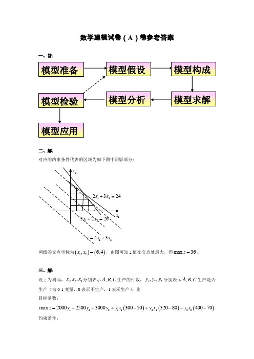
数学建模试卷及参考答案数学建模试卷及参考答案一.概念题(共3小题,每小题5分,本大题共15分)1、一般情况下,建立数学模型要经过哪些步骤(5分)答:数学建模的一般步骤包括:模型准备、模型假设、模型构成、模型求解、模型分析、模型检验、模型应用。
2、学习数学建模应注意培养哪几个能力(5分) 答:观察力、联想力、洞察力、计算机应用能力。
3、人工神经网络方法有什么特点(5分) 答:(1)可处理非线性^;(2)并行结构.;(3)具有学习和记忆能力;(4)对数据的可容性大;(5)神经网络可以用大规模集成电路来实现。
二、模型求证题(共2小题,每小题10分,本大题共20分)1、某人早8:00从山下旅店出发,沿一条路径上山,下午5:00到达山顶并留宿.次日早8:00沿同一路径下山,下午5:00回到旅店.证明:这人必在2天中同一时刻经过路途中某一地点(15分) `证明:记出发时刻为t=a,到达目的时刻为t=b,从旅店到山顶的路程为s.设某人上山路径的运动方程为f(t), 下山运动方程为g(t),t 是一天内时刻变量,则f(t),g(t)在[a,b]是连续函数。
作辅助函数F(t)=f(t)-g(t),它也是连续的,则由f(a)=0,f(b)>0和g(a)>0,g(b)=0,可知F (a )<0, F(b)>0, 由介值定理知存在t0属于(a,b)使F(t0)=0, 即f(t0)=g(t0) 。
2、三名商人各带一个随从乘船过河,一只小船只能容纳二人,由他们自己划行,随从们秘约,在河的任一岸,一旦随从的人数比商人多,就杀人越货,但是如何乘船渡河的大权掌握在商人们手中,商人们怎样才能安全渡河呢(15分) {解:模型构成记第k 次渡河前此岸的商人数为k x ,随从数为k y ,k=1,2,........,k x ,k y =0,1,2,3。
将二维向量k s =(k x ,k y )定义为状态。
安全渡河条件下的状态集合称为允许状态集合,记做S 。
数学建模 建模答案.docx
programi :(1) function [accum, varargout] = CircularHough_Grd(img, radrange, varargin) %Detect circular shapes in a grayscale image. Resolve their center %positions and radii.%% [accum, circen, cirrad, dbg_LMmask] = CircularHough_Grd(% img, radrange, grdthres, fltr4LM_R, multirad, fltr4accum)% Circular Hough transform based on the gradient field of an image.% NOTE: Operates on grayscale images, NOT B/W bitmaps.% NO loops in the implementation of Circular Hough transform,% which means faster operation but at the same time larger% memory consumption.%%%%%%%%% INPUT: (img, radrange, grdthres, fltr4LM_R, multirad, fltr4accum) % % img: A 2-D grayscale image (NO B/W bitmap)%% radrange: The possible minimum and maximum radii of the circles% to be searched, in the format of% [minimum radius , maximum_radius] (unit: pixels)% **NOTE**: A smaller range saves computational time and% memory.%% grdthres: (Optional, default is 10, must be non-negative)% The algorithm is based on the gradient field of the% input image. A thresholding on the gradient magnitude% is performed before the voting process of the Circular% Hough transform to remove the Uniform intensity'% (sort-of) image background from the voting process.% In other words, pixels with gradient magnitudes smaller% than 'grdthres' are NOT considered in the computation.% **NOTE**: The default parameter value is chosen for% images with a maximum intensity close to 255. For cases% with dramatically different maximum intensities, e.g.% 10-bit bitmaps in stead of the assumed 8-bit, the default% value can NOT be used. A value of 4% to 10% of the maximum% intensity may work for general cases.%% fltr4LM_R: (Optional, default is 8, minimum is 3)% The radius of the filter used in the search of local% maxima in the accumulation array. To detect circles whose% shapes are less perfect, the radius of the filter needs% to be set larger.%% multirad: (Optional, default is 0.5)% In case of concentric circles, multiple radii may be% detected corresponding to a single center position. This% argument sets the tolerance of picking up the likely% radii values. It ranges from 0.1 to 1, where 0.1% corresponds to the largest tolerance, meaning more radii % values will be detected, and 1 corresponds to the smallest % tolerance, in which case only the "principal" radius will% be picked up.%% fltr4accum: (Optional. A default filter will be used if not given)% Filter used to smooth the accumulation array. Depending % on the image and the parameter settings, the accumulation % array built has different noise level and noise pattern% (e.g. noise frequencies). The filter should be set to an% appropriately size such that ifs able to suppress the% dominant noise frequency.%%%%%%%%% OUTPUT: [accum, circen, cirrad, dbg_LMmask]%% accum: The result accumulation array from the Circular Hough% transform. The accumulation array has the same dimension % as the input image.%% circen: (Optional)% Center positions of the circles detected. Is a N-by-2% matrix with each row contains the (x, y) positions% of a circle. For concentric circles (with the same center% position), say k of them, the same center position will% appear k times in the matrix.%% cirrad: (Optional)% Estimated radii of the circles detected. Is a N-by-1% column vector with a one-to-one correspondance to the% output tircen*. A value 0 for the radius indicates a% failed detection of the circle's radius.%% dbg_LMmask: (Optional, for debugging purpose)% Mask from the search of local maxima in the accumulation % array.%%%%%%%%%% EXAMPLE #0:% rawimg = imread('TestImg_CHT_a2.bmp');% tic;% [accum, circen, cirrad] = CircularHough_Grd(rawimg, [15 60]);% toe;% figure(l); imagesc(accum); axis image;% title(,Accumulation Array from Circular Hough Transfbrm,);% figure(2); imagesc(rawimg); colormap(,gray,); axis image;% hold on;% plot(circen(:,l), circen(:,2), *r+');% for k = 1 : size(circen, 1),% DrawCircle(circen(k, 1), circen(k,2), cirrad(k), 32,,b」);% end% hold off;% title([*Raw Image with Circles Detected% '(center positions and radii marked)*]);% figure(3); surf(accum, 'EdgeColoF, hone'); axis ij;% title('3-D View of the Accumulation Array*);%% COMMENTS ON EXAMPLE #0:% Kind of an easy case to handle. To detect circles in the image whose% radii range from 15 to 60. Default values for arguments 'grdthres',% 'fltr4LM_R', 'multirad* and ,fltr4accum, are used.%%%%%%%%%% EXAMPLE #1:% rawimg = imread('TestImg_CHT_a3.bmp');% tic;% [accum, circen, cirrad] = CircularHough_Grd(rawimg, [15 60], 10, 20);% toe;% figure(l); imagesc(accum); axis image;% title(,Accumulation Array from Circular Hough Transfbrm,);% figure(2); imagesc(rawimg); colormap('gray'); axis image;% hold on;% plot(circen(:,l), circen(:,2), T+');% for k = 1 : size(circen, 1),% DrawCircle(circen(k, 1), circen(k,2), cirrad(k), 32, 'b-');% end% hold off;% title([*Raw Image with Circles Detected% '(center positions and radii marked)*]);% figure(3); surf(accum, 'EdgeColoF, hone'); axis ij;% title(*3-D View of the Accumulation Array*);%% COMMENTS ON EXAMPLE #1:% The shapes in the raw image are not very good circles. As a result,% the profile of the peaks in the accumulation array are kind of% 'stumpy', which can be seen clearly from the 3-D view of the% accumulation array, (As a comparison, please see the sharp peaks in % the accumulation array in example #0) To extract the peak positions % nicely, a value of 20 (default is 8) is used for argument 'fltr4LM_R', % which is the radius of the filter used in the search of peaks.%%%%%%%%%% EXAMPLE #2:% rawimg = imread(,TestImg_CHT_b3 .bmp1);% fltr4img = [1 1 1 1 1; 1 2 2 2 1; 1 2 4 2 1; 1 2 2 2 1; 1 1 1 1 1];% fltr4img = fltr4img / sum(fltr4img(:));% imgfltrd = filter2( fltr4img , rawimg );% tic;% [accum, circen, cirrad] = CircularHough_Grd(imgfltrd, [15 80], 8, 10); % toe;% figure(l); imagesc(accum); axis image;% title(,Accumulation Array from Circular Hough Transfbrm,);% figure(2); imagesc(rawimg); colormap('gray'); axis image;% hold on;% plot(circen(:,l), circen(:,2), T+');% for k = 1 : size(circen, 1),% DrawCircle(circen(k, 1), circen(k,2), cirrad(k), 32, 'b-');% end% hold off;% title([*Raw Image with Circles Detected% '(center positions and radii marked)*]);%% COMMENTS ON EXAMPLE #2:% The circles in the raw image have small scale irregularities along % the edges, which could lead to an accumulation array that is bad for % local maxima detection. A 5-by-5 filter is used to smooth out the % small scale irregularities. A blurred image is actually good for the % algorithm implemented here which is based on the image's gradient % field.%%%%%%%%%% EXAMPLE #3:% rawimg = imread('TestImg_CHT_c3.bmp');% fltr4img = [1 1 1 1 1; 1 2 2 2 1; 1 2 4 2 1; 1 2 2 2 1; 1 1 1 1 1];% fltr4img = fltr4img / sum(fltr4img(:));% imgfltrd = filter2( fltr4img , rawimg );% tic;% [accum, circen, cirrad]=...% CircularHough_Grd(imgfltrd, [15 105], 8, 10, 0.7);% toe;% figure(l); imagesc(accum); axis image;% figure(2); imagesc(rawimg); colormap(,gray,); axis image;% hold on;% plot(circen(:,l), circen(:,2), *r+');% for k = 1 : size(circen, 1),% DrawCircle(circen(k, 1), circen(k,2), cirrad(k), 32,,b」);% end% hold off;% title([*Raw Image with Circles Detected% '(center positions and radii marked)*]);%% COMMENTS ON EXAMPLE #3:% Similar to example #2, a filtering before circle detection works for% noisy image too. 'multirad* is set to 0.7 to eliminate the false% detections of the circles* radii.%%%%%%%%%% BUG REPORT:% This is a beta version. Please send your bug reports, comments and% suggestions to pengtao@ . Thanks.%%%%%%%%%%% INTERNAL PARAMETERS:% The INPUT arguments are just part of the parameters that are used by% the circle detection algorithm implemented here. Variables in the code% with a prefix ,prm_, in the name are the parameters that control the% judging criteria and the behavior of the algorithm. Default values for% these parameters can hardly work for all circumstances. Therefore, at% occasions, the values of these INTERNAL PARAMETERS (parameters that% are NOT exposed as input arguments) need to be fine-tuned to make% the circle detection work as expected.% The following example shows how changing an internal parameter could% influence the detection result.% 1. Change the value of the internal parameter 'prm LM LoBndRa* to 0.4% (default is 0.2)% 2. Run the following matlab code:% fltr4accum = [1 2 1; 2 6 2; 1 2 1];% fltr4accum = fltr4accum / sum(fltr4accum(:));% rawimg = imread(,Frame_0_0022jportion.jpg,);% tic;% [accum, circen] = CircularHough_Grd(rawimg,...% [4 14], 10, 4, 0.5, fltr4accum);% toe;% figure(l); imagesc(accum); axis image;% title(*Accumulation Array from Circular Hough Transform*);% figure(2); imagesc(rawimg); colormap(,gray,); axis image;% hold on; plot(circen(:,l), circen(:,2), "); hold off;% title('Raw Image with Circles Detected (center positions marked)*);% 3. See how different values of the parameter 'prm LM LoBndRa* could % influence the result.% Author: Tao Peng% Department of Mechanical Engineering% University of Maryland, College Park, Maryland 20742, USA% pengtao@% Version: Beta Revision: Mar. 07, 2007%%%%%%%% Arguments and parameters %%%%%%%%%%%%%%%%%%%%%%%%%%%%%%%%%%%% Validation of argumentsif ndims(img)〜=2 || 〜isnumeric(img),error(*CircularHough_Grd: "img" has to be 2 dimensionaf);endif 〜all(size(img) >= 32),erro^'CircularHough Grd: "img" has to be larger than 32-by-32');endif numel(radrange)〜=2 || -isnumeric(radrange),error([*CircularHough_Grd: "radrange" has to be \ ...'a two-element vector1]);endprm_r_range = sort(max( [0,0;radrange( 1 ),radrange(2)]));% Parameters (default values)prmgrdthres = 10;prmfltrLMR = 8;prmmultirad = 0.5;funccompucen = true;funccompuradii = true;% Validation of argumentsvapgrdthres = 1;if nargin > (1 + vap_grdthres),if isnumeric(varargin{vap grdthres}) && ...varargin(vap grdthres} (1) >= 0,prm_grdthres = varargin {vapgrdthres} (1);elseerror(['CircularHough_Grd: "grdthres" has to be'a non-negative number1]);endendvap_fltr4LM = 2; % filter for the search of local maximaif nargin > (1 + vap_fltr4LM),if isnumeric(varargin{vap_fltr4LM}) && varargin{vap_fltr4LM}(1) >= 3, prmfltrLMR = varargin{vap_fltr4LM} (1);elseerror([,CircularHough_Grd: n fltr4LM_R n has to belarger than or equal to 3']);endendvap_multirad = 3;if nargin > (1 + vap multirad),if isnumeric(varargin{vap_multirad}) && ...varargin{vap multirad}(1) >= 0.1 && ...varargin {vap multirad} (1) <= 1,prmmultirad = varargin {vap_mul tirad} (1);elseerror(['CircularHough_Grd: "multirad" has to be'within the range [0.1, 1]*]);endendvap_fltr4accum = 4; % filter for smoothing the accumulation arrayif nargin > (1 + vap_fltr4accum),if isnumeric(varargin{vap_fltr4accum}) && ...ndims(varargin{vap_fltr4accum}) == 2 && ...all(size(varargin {vap_fltr4accum}) >= 3),fltr4accum = varargin {vap_fltr4accum};elseerror(['CircularHough_Grd: n fltr4accum n has to be \ ...*a 2-D matrix with a minimum size of 3-by-3']);endelse% Default filter (5-by-5)fltr4accum = ones(5,5);fltr4accum(2:4,2:4) = 2;fltr4accum(3,3) = 6;end func_compu_cen = (nargout > 1 );func_compu_radii = (nargout > 2 );% Reserved parametersdbg on = false; % debug information dbgbfigno = 4;if nargout > 3, dbg on = true; end%%%%%%%% Buildingaccumulation array %%%%%%%%%%%%%%%%%%%%%%%%%%%%%%%%% Convert the image to single if it is not of% class float (single or double) img_is_double = isa(img, double');if ~(img_is_double || isa(img, 'single')),imgf = single(img);end% Compute the gradient and the magnitude of gradientif img_is_double,[grdx, grdy] = gradient(img);else[grdx, grdy] = gradient(imgf);endgrdmag = sqrt(grdx.A2 + grdy.A2);% Get the linear indices, as well as the subscripts, of the pixels% whose gradient magnitudes are larger than the given threshold grdmasklin = find(grdmag > prm_grdthres);[grdmask_ldxl, grdmask_IdxJ] = ind2sub(size(grdmag), grdmasklin);% Compute the linear indices (as well as the subscripts) of% all the votings to the accumulation array.% The Matlab function 'accumarray* accepts only double variable, % so all indices are forced into double at this point.% A row in matrix ,lin2accum_aJ, contains the J indices (into the % accumulation array) of all the votings that are introduced by a % same pixel in the image. Similarly with matrix linZaccum aP. rr_41inaccum = double( prm_r_range );linaccum_dr = [ (-rr_41inaccum(2) + 0.5) : -rr_41inaccum(l),... (rr_41inaccum(l) + 0.5) : rr_41inaccum(2)];lin2accum_aJ = floor(...double(grdx(grdmasklin)./grdmag(grdmasklin)) * linaccum_dr + ...repmat( double(grdmask_IdxJ)+0.5 , [ 1 ,length(linaccum_dr)])...);lin2accum_al = floor(...double(grdy(grdmasklin)./grdmag(grdmasklin)) * linaccum dr + ...repmat( double(grdmask_IdxI)+0.5 , [1 ,length(linaccum_dr)])...);% Clip the votings that are out of the accumulation arraymask_valid_a J al =...lin2accum_aJ > 0 & lin2accum_aJ < (size(grdmag,2) + 1) & ...Iin2accum_al > 0 & lin2accum_al < (size(grdmag,l) + 1);mask_valid_aJaI_reverse =〜mask_valid_aJaI;lin2accum_aJ = lin2accum_aJ .* maskvalida J al + maskvalidaJ alreverse;lin2accum_al = lin2accum_al .* mask_valid_aJaI + mask_valid_aJaI_reverse;clear mask_valid_aJ alre verse;% Linear indices (of the votings) into the accumulation arraylin2accum = sub2ind( size(grdmag), lin2accum_al, lin2accum_aJ );lin2accum_size = size( lin2accum );lin2accum = reshape( lin2accum, [numel(lin2accum),l]);clear lin2accum_al lin2accum_aJ;% Weights of the votings, currently using the gradient maginitudes% but in fact any scheme can be used (application dependent)weight4accum =...repmat( double(grdmag(grdmasklin)) , [lin2accum_size(2), 1 ]) .* ...mask_valid_aJ al(:);clear mask_valid_aJaI;% Build the accumulation array using Matlab function 'accumarray'accum = accumarray( lin2accum , weight4accum );accum = [ accum ; zeros( numel(grdmag) - numel(accum), 1 )];accum = reshape( accum, size(grdmag));%%%%%%%% Locating local maxima in the accumulation array %%%%%%%%%%%%% Stop if no need to locate the center positions of circlesif ~func_compu_cen,return;endclear lin2accum weight4accum;% Parameters to locate the local maxima in the accumulation array% — Segmentation of 'accum' before locating LM prmuseaoi = true;prm_aoithres_s = 2;prm aoiminsize = floor(min([ min(size(accum)) * 0.25,... prm_r_range(2) * 1.5 ]));% — Filter for searching for local maxima prmfltrLMs = 1.35;prm fltrLM r = ceil( prm fltrLM R * 0.6 );prm fltrLM npix = max([ 6, ceil((prm_fltrLM_R/2)A 1.8)]);% — Lower bound of the intensity of local maximaprm LM LoBndRa = 0.2; % minimum ratio of LM to the max of'accum'% Smooth the accumulation arrayfltr4accum = fltr4accum / sum(fltr4accum(:));accum = filter2( fltr4accum, accum );% Select a number of Areas-Of^Interest from the accumulation array if prmuseaoi, % Threshold value for 'accum1prm_llm_thresl = prm_grdthres * prm_aoithres_s;% Thresholding over the accumulation array accummask = ( accum > prm llm thres 1 );% Segmentation over the mask[accumlabel, accum nRgn] = bwlabel( accummask, 8 );% Select AOIs from segmented regionsaccumAOI = ones(0,4);for k = 1 : accum nRgn,accumrgn lin = find( accumlabel = k);[accumrgn_ldxl, accumrgn_IdxJ]=...ind2sub( size(accumlabel), accumrgn lin);rgn top = min( accumrgn ldxl);rgn bottom = max( accumrgn_ldxl);rgn left = min( accumrgn ldxJ );rgn_right = max( accumrgn ldxJ );% The AOIs selected must satisfy a minimum sizeif ((rgn_right - rgn_left + 1) >= prm_aoiminsize && ...(rgn_bottom - rgn top + 1) >= prm aoiminsize ),accumAOI = [ accumAOI;...rgn top, rgn bottom, rgn left, rgn right ];endendelse% Whole accumulation array as the one AOIaccumAOI = [1, size(accum,l), 1, size(accum,2)];end% Thresholding of 'accum' by a lower boundprm LM LoBnd = max(accum(:)) * prm LM LoBndRa;% Build the filter for searching for local maxima fltr4LM = zeros(2 * prm_fltrLM_R + 1);[mesh4fLM_x, mesh4fLM_y] = meshgrid(-prm_fltrLM_R : prm fltrLM R);mesh4fLM_r = sqrt( mesh4fLM_x.A2 + mesh4fLM_y.A2 );fltr4LM_mask =...(mesh4fLM_r > prm_fltrLM_r & mesh4fLM_r <= prm fltrLM R );fltr4LM = fltr4LMfltr4LM_mask * (prm fltrLM s / sum(fltr4LM_mask(:)));if prm_fltrLM_R >= 4,fltr4LM_mask = ( mesh4fLM_r < (prm_fltrLM_r - 1));elsefltr4LM_mask = ( mesh4fLM_r < prm fltrLM r );endfltr4LM = fltr4LM + fltr4LM mask / sum(fltr4LM_mask(:));% **** Debug code (begin)if dbg_on,dbg_LMmask = zeros(size(accum));end% **** Debug code (end)% For each of the AOIs selected, locate the local maximacircen = zeros(0,2);fbrk = 1 : size(accumAOI, 1),aoi = accumAOI(k,:); % just for referencing convenience% Thresholding of 'accum* by a lower boundaccumaoi_LBMask =...(accum(aoi(l):aoi(2), aoi(3):aoi(4)) > prm LM LoBnd );% Apply the local maxima filtercandLM = conv2( accum(aoi( 1):aoi(2), aoi(3):aoi(4)),...fltr4LM, 'same*);candLM mask = ( candLM > 0 );% Clear the margins of 'candLM mask*candLM_mask([l :prm_fltrLM_R, (end-prm_fltrLM_R+l):end], :) = 0;candLM mask(:, [l:prm_fltrLM_R, (end-prm_fltrLM_R+l):end]) = 0;% **** Debug code (begin)if dbg_on,dbg_LMmask(aoi( 1 ):aoi(2), aoi(3):aoi(4))=...dbg_LMmask(aoi( 1 ):aoi(2), aoi(3):aoi(4)) + ...accumaoi LBMask + 2 * candLM mask;end% **** Debug code (end)% Group the local maxima candidates by adjacency, compute the% centroid position for each group and take that as the center% of one circle detected[candLM label, candLM nRgn] = bwlabel( candLM_mask, 8 );fbr ilabel = 1 : candLM nRgn,% Indices (to current AOI) of the pixels in the groupcandgrp masklin = find( candLM label == ilabel);[candgrp_ldxl, candgrp_IdxJ]=...ind2sub( size(candLM label), candgrp masklin );% Indices (to 'accum') of the pixels in the groupcandgrp_ldxl = candgrp_ldxl + ( aoi(l) - 1 );candgrp IdxJ = candgrp IdxJ + ( aoi(3) - 1 );candgrp_idx2acm =...sub2ind( size(accum) , candgrp ldxl, candgrp IdxJ );% Minimum number of qulified pixels in the groupif sum(accumaoi_LBMask(candgrp_masklin)) < prm_fltrLM_npix, continue;end% Compute the centroid positioncandgrp_acmsum = sum( accum(candgrp_idx2acm));cc_x = sum( candgrp IdxJ .* accum(candgrp_idx2acm) ) / ...candgrpacmsum;cc_y = sum( candgrp_ldxl .* accum(candgrp_idx2acm) ) / ...candgrpacmsum;circen = [circen; cc_x, cc_y];endend% **** Debug code (begin)if dbg_on,figure(dbg bfigno); imagesc(dbg LMmask); axis image;title(*Generated map of local maxima1);if size(accumAOI, 1) == 1,figure(dbg_bfigno+1);surf(candLM, 'EdgeColor1, hone'); axis ij;title(,Accumulation array after local maximum filtering*);endend% **** Debug code (end)%%%%%%%% Estimation of the Radii of Circles %%%%%%%%%%%%% Stop if no need to estimate the radii of circlesif ~func_compu_radii,varargout{l} = circen;return;end% Parameters for the estimation of the radii of circlesfltr4SgnCv=[2 1 1];fltr4SgnCv = fltr4SgnCv / sum(fltr4SgnCv);% Find circle's radius using its signature curve cirrad = zeros( size(circen,l), 1 );for k = 1 : size(circen,l),% Neighborhood region of the circle for building the sgn. curve circen_round = round( circen(k,:));SCvR IO = circen_round(2) - prm_r_range(2) - 1;ifSCvR_IO<l,SCvR_I0= 1;endSCvRIl = circen_round(2) + prm_r_range(2) + 1;if SCvR Il > size(grdx,l),SCvRIl = size(grdx,l);endSCvR JO = circen round(l) - prm_r_range(2) - 1;ifSCvR_JO<l,SCvRJO = 1;endSCvRJ 1 = circenround(l) + prm_r_range(2) + 1;if SCvR Jl > size(grdx,2),SCvRJl = size(grdx,2);end% Build the sgn. curveSgnCvMat_dx = repmat( (SCvR J0:SCvR J 1) - circen(k,l),...[SCvRJl - SCvRJO +1,1]);SgnCvMat_dy = repmat( (SCvR_IO:SCvR_Il)' - circen(k,2),...[1 , SCvRJl - SCvRJO + 1]);SgnCvMat_r = sqrt( SgnCvMat dx .A2 + SgnCvMat_dy .A2 );SgnCvMatrpl = round(SgnCvMatr) + 1;f4SgnCv = abs(...double(grdx(SCvR_IO:SCvR_Il, SCvRJO:SCvRJ 1)) .* SgnCvMat_dx + ...double(grdy(SCvR_IO:SCvR Il, SCvR JO:SCvR J 1)) .* SgnCvMat dy...)./ SgnCvMat r;SgnCv = accumarray( SgnCvMat rp 1(:) , f4SgnCv(:));SgnCv_Cnt = accumarray( SgnCvMat rp 1 (:) , ones(numel(f4SgnCv), 1));SgnCv_Cnt = SgnCv_Cnt + (SgnCv_Cnt == 0);SgnCv = SgnCv ./ SgnCv_Cnt;% Suppress the undesired entries in the sgn. curve% ― Radii that correspond to short arcsSgnCv = SgnCv .* ( SgnCv_Cnt >= (pi/4 * [O:(numel(SgnCv_Cnt)-1 )]*));% ― Radii that are out of the given rangeSgnCv( 1 : (round(prm_r_range( 1))+1) ) = 0;SgnCv( (round(prm_r_range(2))+1) : end ) = 0;% Get rid of the zero radius entry in the arraySgnCv = SgnCv(2:end);% Smooth the sgn. curveSgnCv = filtfilt( fltr4SgnCv , [1] , SgnCv );% Get the maximum value in the sgn. curveSgnCv_max = max(SgnCv);if SgnCv_max <= 0,cirrad(k) = 0;continue;end% Find the local maxima in sgn. curve by 1st order derivatives% ― Mark the ascending edges in the sgn. curve as Is and% ― descending edges as OsSgnCv AscEdg = ( SgnCv(2:end) - SgnCv(l:(end-l)) ) > 0;% ― Mark the transition (ascending to descending) regionsSgnCv LMmask = [ 0; 0; SgnCv_AscEdg(l:(end-2)) ] & (〜SgnCv_AscEdg);SgnCv LMmask = SgnCvLMmask & [ SgnCv_LMmask(2:end); 0 ];% Incorporate the minimum value requirementSgnCvLMmask = SgnCvLMmask & ...(SgnCv(l:(end-l)) >= (prm_multirad * SgnCv_max));% Get the positions of the peaksSgnCv LMPos = sort( find(SgnCv_LMmask));% Save the detected radiiif isempty(SgnCvLMPos),cirrad(k) = 0;elsecirrad(k) = SgnCvLMPos(end);for i radii = (length(SgnCv LMPos) - 1) : -1 : 1,circen = [ circen; circen(k,:)];cirrad = [ cirrad; SgnCv_LMPos(i_radii)];endendend% Outputvarargout{l} = circen;varargout{2} = cirrad;if nargout > 3,varargout{3} = dbg_LMmask;endprograms:programs:2 function DrawCircle (x, y, r, nseg, S)% Draw a circle on the current figure using ploylines%% DrawCircle (x, y, r, nseg, S)% A simple function for drawing a circle on graph.%% INPUT: (x, y, r, nseg, S)% x, y: Center of the circle% r: Radius of the circle% nseg: Number of segments for the circle% S: Colors, plot symbols and line types%% OUTPUT: None%% BUG REPORT:% Please send your bug reports, comments and suggestions to% pengtao@glue. umd. edu . Thanks.% Author: Tao Peng% Department of Mechanical Engineering% University of Maryland, College Park, Maryland 20742, USA % pengtao@glue. umd. edu% Version: alpha Revision: Jan. 10, 2006theta = 0 : (2 * pi / nseg) : (2 * pi);pline_x 二r * cos(theta) + x;pline_y 二r * sin(theta) + y;plot (pline_x, pline_y, S);3function testiml二imread (' image 1. jpg');% rawimg = imread(,TestImg_CHT_c3. bmp J);rawimg=rgb2gray(iml);tic;[accum, circen, cirrad] = CircularHough_Grd(rawimg, [20 30], 5,50);circentoe;figure(1) ; imagesc(accum); axis image;title (J Accumulation Array from Circular Hough Transform,); figure (2) ; imagesc (rawimg) ; colormap (J gray,) ; axis image; hold on;plot (circen(:, 1), circen(:, 2), ' r+');for k = 1 : size (circen, 1),DrawCircle (circen (k, 1), circen (k, 2), cirrad (k), 32, ' b-'); end hold off; title(f Raw Image with Circles Detected ...'(center positions and radii marked)']);figure (3); surf(accum, ' EdgeColor,, ' none5); axis ij; title (J 3-D View of the Accumulation Array');附带图像image 1. jpg直接运行test.m即可得到上方的结果!当然方法是活的,只要合理即可行。
数学建模复习资料参考答案
《数学建模》复习资料参考答案一、不定项选择1、建模能力包括 A、B、C、D 。
A、理解实际问题的能力B、抽象分析问题的能力C、运用工具知识的能力D、试验调试的能力2、按照模型的应用领域分的模型有 A、E 。
A、传染病模型B、代数模型C、几何模型D、微分模型E、生态模型3、对黑箱系统一般采用的建模方法是 C 。
A、机理分析法B、几何法C、系统辩识法D、代数法4、一个理想的数学模型需满足 A、B 。
A、模型的适用性B、模型的可靠性C、模型的复杂性D、模型的美观性5、按照建立模型的数学方法分的模型有 B、C、D 。
A、传染病模型B、代数模型C、几何模型D、微分模型E、生态模型6、下列说法正确的有 A、C 。
A、评价模型优劣的唯一标准是实践检验。
B、模型误差是可以避免的。
C、生态模型属于按模型的应用领域分的模型。
D、白箱模型意味着人们对原型的内在机理了解不清楚。
7、力学中把 A 的量纲作为基本量纲。
A、质量、长度、时间B、密度、时间、长度C、质量、密度D、时间、长度8、下列说法错误的有 B 。
A、评价模型优劣的唯一标准是实践检验。
B、模型误差是可以避免的。
C、生态模型属于按模型的应用领域分的模型。
D、白箱模型意味着人们对原型的内在机理了解清楚。
9、建立数学模型的方法和步骤有ABCDE。
A、模型假设。
B、模型求解。
C、模型构成。
D、模型建立。
E、模型分析。
10、模型按照替代原型的方式可以简单分为AB。
A、形象模型B、抽象模型C、生态模型D、白箱模型11、形象模型可以具体分为ABC。
A.直观模型B、物理模型C、分子结构模型等;12、抽象模可以具体分为ABC。
A 思维模型B符号模型C数学模型D分子结构模型13建模的一般原则为ABCD。
A目的性原则B简明性原则C真实性原则D全面性原则;14 模型的结构大致分为ABC。
A、灰箱模型B、白箱模型C、黑箱模型15A、建立递阶层次结构模型;B、构造出各层次中的所有判断矩阵;C、层次单排序及一致性检验;D、层次总排序及一致性检验。
数学模型试题及答案解析

数学模型试题及答案解析一、单项选择题(每题3分,共30分)1. 以下哪个不是数学模型的特征?A. 抽象性B. 精确性C. 可验证性D. 复杂性答案:D2. 数学模型的建立通常不包括以下哪个步骤?A. 定义问题B. 收集数据C. 建立假设D. 验证结果答案:D3. 在数学建模中,以下哪个不是模型分析的方法?A. 定性分析B. 数值分析C. 图形分析D. 统计分析答案:D4. 数学模型的验证不包括以下哪项?A. 内部一致性检验B. 与已知结果比较C. 与实验数据比较D. 模型的优化答案:D5. 在数学建模中,以下哪个不是模型的类型?A. 确定性模型B. 随机模型C. 动态模型D. 静态模型答案:D6. 以下哪个是数学模型的典型应用领域?A. 经济学B. 物理学C. 生物学D. 所有以上答案:D7. 数学模型的建立过程中,以下哪个步骤是不必要的?A. 问题定义B. 假设建立C. 模型求解D. 模型展示答案:D8. 数学模型的分析中,以下哪个不是常用的工具?A. 微分方程B. 线性代数C. 概率论D. 量子力学答案:D9. 在数学建模中,以下哪个不是模型的评估标准?A. 准确性B. 可解释性C. 简洁性D. 复杂性答案:D10. 数学模型的建立过程中,以下哪个步骤是至关重要的?A. 问题定义B. 数据收集C. 模型求解D. 模型验证答案:A二、多项选择题(每题5分,共20分)11. 数学模型的建立过程中,以下哪些步骤是必要的?A. 问题定义B. 数据收集C. 模型求解D. 模型验证答案:ABCD12. 数学模型的类型包括以下哪些?A. 确定性模型B. 随机模型C. 动态模型D. 静态模型答案:ABCD13. 数学模型的分析方法包括以下哪些?A. 定性分析B. 数值分析C. 图形分析D. 统计分析答案:ABCD14. 数学模型的验证包括以下哪些?A. 内部一致性检验B. 与已知结果比较C. 与实验数据比较D. 模型的优化答案:ABC三、填空题(每题4分,共20分)15. 数学模型的建立通常包括定义问题、______、建立假设和模型求解四个步骤。
《数学建模与数学探究》试卷及答案_高中数学选择性必修第二册_苏教版_2024-2025学年
《数学建模与数学探究》试卷(答案在后面)一、单选题(本大题有8小题,每小题5分,共40分)1、数学建模的一般步骤是以下哪一个顺序?A、模型假设、模型准备、模型求解、模型应用B、模型准备、模型假设、模型求解、模型应用C、模型准备、模型求解、模型假设、模型应用D、模型求解、模型假设、模型准备、模型应用2、下列函数中属于偶函数的是:A.(f(x)=x2+1)B.(f(x)=x3+2))C.(f(x)=1xD.(f(x)=√x2)3、在解决实际问题时,以下哪个选项不属于数学建模的基本步骤?A、建立数学模型B、求解数学模型C、分析结果并验证模型的有效性D、收集数据,进行实验研究4、在建立数学模型时,如果模型的结果与实际情况存在较大的偏差,首先应该()A、直接放弃该模型B、检查数据的准确性和完整性C、重新设定模型参数D、改变模型的数学方法5、已知某地区某种疾病的发病率是0.001,该疾病检测的准确率为99%,即若一个人患病,则检测呈阳性的概率为99%;若未患病,检测结果呈阴性的概率也是99%。
现有一人检测结果为阳性,求此人确实患有该病的概率是多少?A. 99%B. 50%C. 9.9%D. 0.99%6、某学校为了加强学生的环保意识,计划在每个教室种植5株不同种类的植物。
如果学校共有32个教室,且学校已经有200株植物备用,那么还需要从市场上采购多少株植物才能满足需求?A. 30株B. 40株C. 50株D. 60株7、假设一个电子工厂生产一种新型手机,已知每生产一部手机的直接成本为300元,固定成本(包括管理费用、折旧等)为每月5000元。
如果每月生产制品500部,那么每部手机的利润是多少元?A. 200元B. 250元C. 300元D. 350元8、已知某商品的成本函数为(C(x)=0.05x2+3x+200),其中(x)代表生产数量(单位:件)。
如果每件商品的售价为(P=100−0.1x)元,那么为了获得最大利润,应该生产多少件商品?A. 100B. 150C. 200D. 250二、多选题(本大题有3小题,每小题6分,共18分)1、以下哪些是数学建模的基本步骤?A、提出问题B、建立模型C、分析模型D、求解模型E、检验与改进2、在数学建模过程中,选择合适的参数至关重要。
(完整版)数学建模试卷(附答案)
2.设银行的年利率为0.2,则五年后的一百万元相当于现在的 万元.3.在夏季博览会上,商人预测每天冰淇淋销量N 将和下列因素有关: (1)参加展览会的人数n ;(2)气温T 超过10℃;(3)冰淇淋的售价由此建立的冰淇淋销量的比例模型应为 。
二、简答题:(25分)1、建立数学模型的基本方法有哪些?写出建模的一般步骤。
(5分)2、 写出优化模型的一般形式和线性规划模型的标准形式。
(10分) 三、(每小题15分,共60分)1、设某产品的供给函数)(p ϕ与需求函数)(p f 皆为线性函数: 9)(,43)(+-=+=kp p f p p ϕ其中p 为商品单价,试推导k 满足什么条件使市场稳定。
2、1968年,介壳虫偶然从澳大利亚传入美国,威胁着美国的柠檬生产。
随后,美国又从澳大利亚引入了介壳虫的天然捕食者——澳洲瓢虫。
后来,DDT 被普通使用来消灭害虫,柠檬园主想利用DDT 进一步杀死介壳虫。
谁料,DDT 同样杀死澳洲瓢虫。
结果,介壳虫增加起来,澳洲瓢虫反倒减少了。
试建立数学模型解释这个现象。
3.建立捕鱼问题的模型,并通过求解微分方程的办法给出最大的捕捞量数学建模 参考答案2.约40.18763.p T Kn N /)10(-=,(T ≥10℃),K 是比例常数 二、1、建立数学模型的基本方法:机理分析法,统计分析法,系统分析法2、优化模型的一般形式将一个优化问题用数学式子来描述,即求函数 ,在约束条件下的最大值或最小值,其中 为设计变量(决策变量), 为目标函数为可行域三、1、解:设Pn 表示t=n 时的市场价格,由供求平衡可知:)()(1n n p f p =-ϕ9431+-=+-n n kp p即: kp k p n n 531+-=- .,...,,,)(m i h i 210==x )(x f u =.,...,,),)(()(p i g g i i 2100=≥≤x x x)(x f Ω∈x Ω∈=x x f u )(max)min(or .,...,,,)(..m i h t s i 210 ==x .,...,,),)(()(p i g g i i 2100=≥≤x x经递推有:kk p kkk k p k p n nn nn n 5)3()3(5)53(31102⋅-+⋅-=++-⋅-=-=-∑Λ0p 表示初始时的市场价格:∞→时当n 若即市场稳定收敛则时,,30,13n p k 即k<<<-。